Submitted:
05 February 2026
Posted:
06 February 2026
You are already at the latest version
Abstract
Aiming at the problem of accurate estimation of coherent parameters for the distributed coherent jamming system (DCJS), this paper first establishes a transmit-receive signal model of the DCJS in the presence of coherent parameter estimation errors. Then, it analyzes and verifies that the generalized cross-correlation function weighting method causes a decrease in the estimation accuracy of coherent parameters due to whitening processing, which in turn impairs the synthesis efficiency of the DCJS. Finally, a coherent parameter estimation method based on frequency-domain feature matching is proposed. The weighting method based on frequency-domain feature matching can effectively preserve the intra-pulse features of signals, thereby improving the estimation accuracy of coherent parameters. Simulation results show that, compared with the existing algorithms, the proposed method improves the time delay estimation accuracy by 30% and the phase difference estimation accuracy by 7.7%.
Keywords:
distributed coherent jamming system(DCJS)
; coherent parameters estimation
; generalized cross-correlation
; synthesis efficiency
1. Introduction
Distributed coherent jamming is a crucial research direction in the field of electronic warfare, and accurate estimation of coherent parameters is the prerequisite and core for achieving its excellent performance. Based on the distributed coherent synthesis technology [1], the Distributed Coherent Jamming System (DCJS) enables each distributed aperture to conduct accurate estimation of parameters such as time delay and phase difference for the received radar signals. According to the parameter estimation results, the transmission time and phase of jamming emission signals are precisely controlled to ensure that all jamming emission signals can arrive at the radar target simultaneously and in-phase and achieve coherent synthesis. The primary objective of the DCJS is to realize the multiplication of jamming power of each distributed aperture (the jamming power can be increased by a factor of N2 when N jammers with the same effective radiated power are synthesized via distributed coherent technology), which can effectively address the bottleneck that the effective radiated power of a single jammer is difficult to further improve due to restrictions from installation space, weight, power supply and other factors.
DCJS and distributed coherent aperture radar (DCAR) share many similarities, with the core issue being the estimation of CPs [2]. For DCAR to achieve fully coherent operation, the system first transmits orthogonal signals to accurately estimate time differences and phase differences. Based on the CPs estimation results, the system performs time and phase compensation on the received signals to achieve receive coherence. Then, the system transmits the same waveform and adjusts the transmission time and phase using the obtained CPs estimates to achieve transmit coherence, and again uses the received signals to update the CPs, performing time and phase compensation on the received signals to achieve full coherence [3,4,5,6,7].
However, the estimation of coherent parameters for the DCJS is entirely different from that for distributed coherent radar, and few open literatures have reported research on the coherent parameter estimation of DCJS. By utilizing the spatiotemporal two-dimensional synchronous focusing characteristic of time-reversed electromagnetic waves, Chen Qiuju et al. systematically proposed a spatial power synthesis method based on sparse arrays, and carried out simulation analyses on the synthesis efficiency for single-frequency continuous wave signals, pulse signals and linear frequency-modulated signals. Meanwhile, they proved that the spatial power synthesis method based on time reversal is also applicable to moving platforms [8,9,10,11,12,13,14,15].
Cross-correlation-based methods can achieve an estimation accuracy approaching the Cramér-Rao bound under high signal-to-noise ratio (SNR) conditions, whereas their performance degrades drastically in high-noise environments. To mitigate the impact of Gaussian noise on time delay estimation results, Xing Yuhua et al. proposed a method combining singular spectrum decomposition with an improved generalized cross-correlation algorithm. Experimental verification via multiple simulations under a -5 dB Gaussian noise environment demonstrated that, compared with the second-order correlation method, the absolute value of the main peak-to-sidelobe ratio is increased by more than 0.6756 dB. However, singular value decomposition involves extensive matrix operations, which makes it difficult to meet the real-time requirements of electronic warfare systems [16]. To address the issue of noise interference on the phase spectrum, Guan Yu et al. proposed an improved generalized cross-correlation method based on frequency-domain threshold processing. By setting a threshold on the amplitude spectrum prior to the weighting function operation, only the components of the cross-power spectrum function with an amplitude exceeding the threshold are retained in the frequency domain, thereby reducing the impact of noise on the phase spectrum. Nevertheless, this method is only applicable to narrowband signals, and its performance in coherent parameter estimation for wideband signals is not analyzed in the relevant literature [17,18].
Aiming at the problems of poor noise adaptability, low real-time performance and unsatisfactory estimation accuracy for practical applications existing in the current coherent parameter estimation methods, this paper proposes a feasible improved method for coherent parameter estimation on the basis of the research into the generalized cross-correlation method, and verifies the effectiveness and feasibility of the proposed improved method via simulation experiments.
2. Materials and Methods
This section elaborates on the proposed coherent parameter estimation method for improving the frequency-domain weighting function based on frequency-domain feature matching. Section 2.1 describes the transmit-receive signal model of the distributed coherent jamming system (DCJS) in the presence of coherent parameter estimation errors and derives the Cramér-Rao bound for coherent parameter estimation. Section 2.2 describes the conventional coherent parameter estimation method based on the generalized cross-correlation function, presents the method for improving the frequency-domain weighting function via frequency-domain feature matching, and performs coherent parameter estimation using the improved frequency-domain weighting function.
2.1. Signal Model of the Distributed Coherent Jamming System
The schematic diagram of the jamming operation against radar implemented by a DCJS composed of two jamming units is illustrated in Figure 1. At time T0, the radial distance between jamming unit 1 and the radar target is ; jamming unit 1 moves at a constant speed , with a radial velocity relative to the radar target of . The radial distance between jamming unit 2 and the radar target is ; jamming unit 2 moves at a constant speed , with a radial velocity relative to the radar target of . The initial distance difference between the two jamming units and the radar target is .
The signal transmitted by the radar target is expressed as follows:
Wherein: denotes the signal amplitude, ; represents the radar transmitter power; is the radar antenna gain; stands for the radar transmitting antenna impedance; is the baseband signal; denotes the signal pulse width; represents the signal frequency modulation slope, ; is the signal bandwidth; stands for the signal carrier frequency; and is time.
The signal transmitted by the radar target propagates through space and reaches the two jamming units respectively. Due to the independent clocks and local oscillators of the two jamming units, there exist time and phase synchronization errors. Assuming that the time synchronization error of jamming unit 2 relative to jamming unit 1 is and the phase synchronization error is , the signals received by the two jamming units are respectively:
Wherein: and , with denoting the propagation speed of electromagnetic waves; represents the transmission loss corresponding to the propagation path of jamming unit 1, where and is the receiving antenna impedance of jamming unit 1, is the receiving antenna gain of jamming unit 1; stands for the transmission loss corresponding to the propagation path of jamming unit 2, where, is the receiving antenna impedance of jamming unit 2, and is the receiving antenna gain of jamming unit 2.
Define the CPs and , where denotes the time difference between the radar signals received by the two jamming units, and represents the phase difference between the radar signals received by the two jamming units. Thus, we have:
Wherein: , .
To ensure the distributed jamming system operates coherently, the jamming signals transmitted by the two jamming units must arrive simultaneously and in-phase at the phase center of the radar antenna. Clearly, the two jamming units need to compensate for the time delay and phase difference of the transmitted signals based on the received radar signals. Specifically, parameter estimation of Δτ and Δφ is required; during jamming transmission, the time delay and phase difference of the signals transmitted by the two units are controlled according to the estimated values of and . The higher the estimation accuracy of and , the better the coherent combining performance.
Define the unknown parameter vector as follows:
Assume that the estimated value of the unknown parameter vector is , and it holds that:
Wherein: and are the estimated values of and respectively; ; ; and and represent the estimation errors of time delay and phase difference respectively.
Based on the above definition of CPs, the time and phase parameters to be estimated are relative values rather than absolute values. During jamming transmission, it is only necessary to take one jamming unit as a reference and ensure the relative time and phase relationships between other jamming units and the reference unit. For jamming transmission, the signal transmitted by jamming unit 1 is taken as the reference, and the time delay and phase of jamming unit 2 are compensated. Let the time compensation amount be and the phase compensation amount be . Then, the transmitted signals of jamming units 1 and 2 are respectively:
Wherein: and denote the amplitude modulation coefficients of jamming units 1 and 2 respectively. Substituting and into and respectively, we obtain:
Assume that the jamming response times of the two jamming units are identical, denoted as . Within the time , the change in radial distance between jamming unit 1 and the radar is , with the corresponding propagation delay variation being ; the change in radial distance between jamming unit 2 and the radar is , with the corresponding propagation delay variation being . Thus, the combined signal of the transmitted signals from the two jamming units at the radar target is:
Wherein: denotes the propagation loss corresponding to the transmission path from jamming unit 1 to the radar, and represents the propagation loss corresponding to the transmission path from jamming unit 2 to the radar. Substituting and (the transmitted signals of the two jamming units) into the combined signal expression respectively, and defining , , , , we obtain:
To ensure the two jamming signals are combined simultaneously and in-phase, the following condition must be satisfied:
That is:
Substituting and according to Equations (4) and (5), we obtain:
Substituting Equations (16) and (17) into Equation (13), we get:
After receiving the signal, the radar performs matched filtering processing to obtain the output signal after pulse compression. The impulse response of the matched filter is the time-reversed conjugate of the transmitted baseband signal:
Then, the output signal of this signal after passing through the matched filter is:
Substituting and into the equation, we obtain:
After simplification, we can obtain:
After passing through the matched filter, the carrier frequency of the output signal is , and the envelope modulation is a sinc function.
Due to the existence of an estimation error between the time difference and its estimated value , as well as an estimation error between the phase difference and its estimated value , the two jamming signals cannot be completely superimposed at the radar target, leading to energy loss. Substituting Equations (18) and (19) into Equation (13) respectively, we obtain:
Substitute the estimated values and of and into the above equation respectively, and the actual superimposed signal at the phase center of the radar antenna is obtained:
Substitute , , , and into the above equation, and after simplification, we obtain:
The output signal of this signal after passing through the matched filter is:
Substitute and into , and we obtain:
After simplification, we obtain:
When the time difference between the two jamming signals is greater than the radar’s time delay resolution, the radar will distinguish the two jamming signals as two separate targets. In this case, discussing the coherent synthesis efficiency is meaningless. The time delay resolution of the radar is ; therefore, the coherent synthesis efficiency should be discussed under the condition , i.e., . The coherent synthesis efficiency is defined as:
Substitute and respectively, and after simplification, we obtain:
Wherein: is the Fourier transform of , is the energy of the signal , and .
Obviously, when and , the coherent synthesis efficiency . Under different error conditions, a simulation analysis was performed on the coherent synthesis efficiency. The following assumptions are made: the distance between the two jamming units is 1000 m; the distance between Jamming Unit 1 and the radar target is 100 km; the distance between Jamming Unit 2 and the radar target is 100.1 km; the radar signal adopts linear frequency modulation (LFM), with a carrier frequency of 6 GHz, a bandwidth of 10 MHz, a pulse width of 10 μs, and a pulse repetition period (PRP) of 1 ms. The simulation results of the relationship between the time delay estimation error and the coherent synthesis efficiency are shown in the figure below.
Figure 2.
Curves of coherent synthesis efficiency versus time delay error and phase difference error.
Figure 2.
Curves of coherent synthesis efficiency versus time delay error and phase difference error.
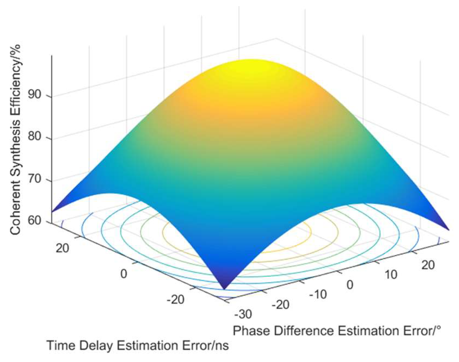
Figure 3.
Error curves when coherent synthesis efficiency Is 80%.
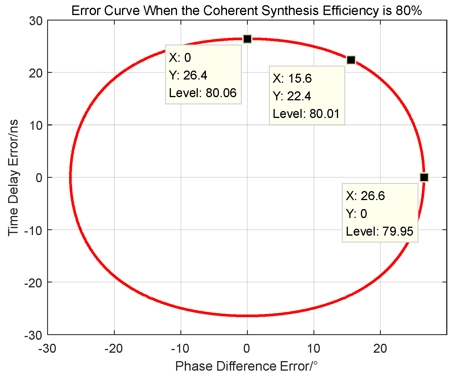
Based on the above simulation results, the smaller the estimation errors of time delay and phase difference, the higher the coherent synthesis efficiency. Specifically, to achieve a coherent synthesis efficiency of 80%: when the time delay estimation error is 0, the phase difference estimation error should be no more than 26.6°; when the phase difference estimation error is 0, the time delay estimation error should be no more than 26.4ns; if the phase difference estimation error is 15.6°, the time delay estimation error should be no more than 22.4ns. It can be seen that the estimation errors of time delay and phase difference directly affect the coherent synthesis efficiency. To achieve the coherent synthesis efficiency meeting the specified requirements, the estimation accuracy of time delay and phase difference must be controlled.
The Cramér-Rao low-bound (CRLB) for time delay and phase difference estimation can be readily derived as follows:
According to the above results, the CRLBs of time delay and phase difference have no correlation with the time synchronization accuracy and phase synchronization accuracy . This seems contradictory to intuitive understanding, because generally, the worse the synchronization accuracy, the lower the estimation accuracy of time delay and phase difference will inevitably be. In fact, the time synchronization accuracy and phase synchronization accuracy between jamming units were taken into account in the above analysis. However, when solving the FIM, and were analyzed as an integrated whole, thus avoiding the impact of and . Actually, the estimated parameters in the analysis are the estimates of the true time delay value and the true phase difference value . Specifically, the time delay estimation includes both the time delay caused by path difference and the time delay caused by clock asynchrony, while the phase difference estimation includes both the phase difference caused by path difference and the phase difference caused by clock asynchrony. Therefore, the obtained CRLBs of time delay and phase difference are independent of synchronization accuracy. In practice, however, synchronization errors is inevitably present in distributed coherent jamming systems. When adopting various coherent parameter estimation algorithms, the impact of synchronization accuracy on coherent parameter estimation must be considered.
2.2. Improvements to Coherent Parameter Estimation Method
On the basis of the traditional cross-correlation(CC) algorithm, the generalized cross-correlation(GCC) algorithm introduces frequency-domain weighting processing to suppress noise interference and enhance the effective components of signals. Its core idea is to perform frequency-domain pre-filtering on the two received signals, and then extract the time delay estimation value and phase difference estimation value through cross-correlation operation.
According to the Wiener-Khinchin theorem, the Fourier transform of a CC function is the cross-power spectrum of two signals; thus, we have:
Wherein, is the cross-power spectral function of and . Denoting and as the Fourier transforms of and respectively, we have . To suppress frequency-domain noise, a weighting function is introduced to filter the cross-power spectral function , resulting in the weighted cross-power spectral function [26]:
According to the different construction methods of , commonly used weighting functions include the Phase Transform (PHAT), Smoothed Coherence Transform (SCOT), and Roth Weighting (ROTH).
The weighting function of the PHAT method is the reciprocal of the modulus of the cross-power spectral function, i.e.,:
The PHAT method leverages the relationship between time delay and phase difference, i.e., . By directly normalizing the amplitude of the cross-power spectral function at all frequency points (a straightforward approach) and retaining only phase information, it can form a sharper cross-correlation function peak in the time domain. This is equivalent to performing whitening filtering on the signal. Under ideal conditions, the inverse Fourier transform of the cross-power spectral function weighted by PHAT is a Dirac delta function: the position corresponding to the peak is the time delay, and the phase corresponding to the peak is the phase difference—thereby enhancing the robustness of parameter extraction.
The PHAT method requires two FFT operations and one IFFT operation, with a computational complexity of . However, the PHAT method completely discards amplitude information, which weakens the effective signal components and makes it sensitive to noise. Weighting amplifies phase errors in the noise frequency band, leading to an increase in the variance of time delay estimation.
The weighting function of the SCOT method is the reciprocal of the square root of the product of the auto-power spectra of the two signals, i.e.,:
Wherein, and .
The SCOT method can eliminate frequency-domain distortion by normalizing the auto-power spectra of the two signals, allowing the CC function to focus more on time delay information. The weighted cross-power spectrum is equivalent to a coherence function, which reflects the linearity of the two signals at each frequency point. This enables the suppression of incoherent noise interference, making the SCOT method suitable for scenarios with frequency dispersion and capable of mitigating the impact of frequency-selective fading on time delay estimation. The computational complexity of the SCOT method is . Similarly, the SCOT method suffers from noise sensitivity: at low SNR, the auto-power spectrum estimation is contaminated by noise, resulting in degraded performance.
The ROTH method was first proposed in 1971 by Stanley A. Roth, a researcher from the Lincoln Laboratory at the Massachusetts Institute of Technology (MIT). Its weighting function is the reciprocal of the auto-power spectral function of the reference signal [27], i.e.,:
The core idea of the ROTH method is to suppress interference in noise-dominant frequency bands by normalizing the auto-power spectral function of the reference signal. Essentially, it assumes that noise mainly exists in the reference signal; through weighting, it suppresses the impact of low-noise frequency bands on cross-correlation. In the effective frequency bands of the signal (i.e., frequency bands with relatively high SNR), the weighted cross-power spectral function is approximately equal to , which preserves the phase difference and time delay information of the two signals.
The computational complexity of the ROTH method is . The ROTH method is suitable for scenarios where noise mainly exists in while the noise in is weak. It relies on the prior estimation of the noise power spectrum of the reference signal; otherwise, the weighting may fail.
To intuitively demonstrate the effectiveness of each weighting method, the figure below presents the simulation results of comparing the CC functions of each weighting method and the conventional CC method under the ideal no-noise condition and at a SNR of 10 dB.
Figure 4.
Comparison of CC functions between various weighting methods and the conventional CC method (a) Ideal condition (b) SNR = 10 dB.
Figure 4.
Comparison of CC functions between various weighting methods and the conventional CC method (a) Ideal condition (b) SNR = 10 dB.
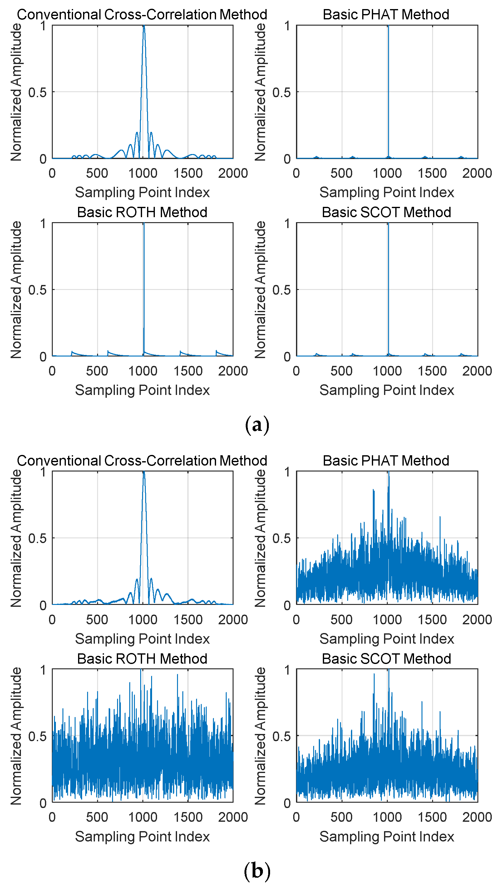
As can be seen from Figure 8(a), under ideal conditions, compared with the conventional cross-correlation function method, all weighting methods achieve the effect of peak sharpening to varying degrees. It can be observed from Figure 8(b) that when the SNR is 10dB, affected by noise, the noise floors of the CC functions of each weighting method rise to different extents. Among them, the ROTH method performs the worst, with its peak completely submerged by noise; the PHAT and SCOT methods perform slightly better. However, surprisingly, the conventional GCC method is almost unaffected by noise. Does this indicate that the generalized cross-correlation algorithm with frequency-domain weighting is ineffective? Actually, it does not.
As analyzed earlier, each weighting algorithm has its own distinct characteristics and applicable scenarios:
The ROTH method assumes that noise primarily exists in , which clearly does not align with the scenario of this study. In the scenario of this paper, it is assumed that there is additive white Gaussian noise (AWGN) with independent and identical distribution (i.i.d.) in both and ; therefore, it is understandable that the ROTH method yields the worst performance.
The PHAT method performs whitening processing on the cross-power spectrum, which results in the loss of amplitude information at the target signal frequency. Consequently, the cross-correlation signal fails to obtain pulse compression gain, leading to degraded performance when the SNR is not high.
The SCOT method normalizes the auto-power spectra of the two signals. In the scenario of this paper, the spectra of the two signals are consistent; thus, similar to the PHAT method, the CC signal loses pulse compression gain.
In contrast, the traditional CC algorithm can obtain full pulse compression gain. When the pulse width Tp is 10μs and the bandwidth B is 10MHz, an equivalent gain of 20dB is achieved. Therefore, its performance is far superior to that of other frequency-domain weighted normalization algorithms.
In principle, the method of sharpening the CC function through frequency-domain weighting and normalization can certainly improve the robustness of time delay and phase difference estimation. However, the problem is that the above weighting algorithms discard the amplitude information in the frequency domain for both noise and signals through normalization, which will inevitably lead to corresponding losses. If we can only normalize the noise in the frequency domain while retaining the amplitude information of the useful frequency bands of the signal, it should be possible to improve the accuracy of parameter estimation.
For a linear frequency-modulated (LFM) signal, under ideal conditions, the amplitude and phase characteristics of the cross-power spectrum are shown in the following figure. It can be seen that the amplitude of the cross-power spectrum is approximately rectangular, and the phase varies linearly with frequency. This is because the cross-power spectrum includes the phase difference term . Therefore, when the time delay is fixed, changes linearly with frequency, with a slope of . Theoretically, the time delay value can be obtained by differentiating the phase of the cross-power spectrum, but this method has high requirements for the SNR [28].
Based on the cross-power spectral function of the two signals, the noise floor power is estimated, and a reference threshold is set according to the noise floor power estimation result. This threshold is used to protect the effective frequency bands of the signals: frequency-domain weighting processing is applied to frequency points whose power does not exceed the threshold, while frequency points whose power exceeds the threshold remain unchanged. By improving each weighting method, the following weighting functions are obtained:
Wherein, is the noise power threshold.
Through the above improved methods, the spectral characteristics of the normalized cross-power function are ensured to match those of the original cross-power spectrum, and the pulse compression gain of the cross-correlation function can be completely retained. Compared with the basic PHAT method, basic SCOT method, and basic ROTH method, the method of improving frequency-domain weighting based on frequency-domain feature matching only adds one comparison operation. The computational complexity of the improved method based on PHAT is , the computational complexity of the improved method based on ROTH is , and the computational complexity of the improved method based on SCOT is .
3. Simulation-Based Verification
Based on the improved weighting functions, simulation and analysis were conducted on the CC functions and cross-power spectra of the PHAT-based improved method, ROTH-based improved method, and SCOT-based improved method respectively. The signal parameters were set as follows: the pulse width Tp was 10μs, the bandwidth B was 10MHz, the sampling rate was 50B (i.e., 500 MHz) corresponding to a sampling interval of 2ns, the data length N was 1000, the phase synchronization error was 30°, the time synchronization error was 5ns, and the SNR were 0 dB and 10 dB respectively. The simulation results are shown in the figures below; in each subfigure, the abscissa represents the number of sampling points, and the ordinate represents the normalized amplitude.
Figure 5.
Comparison of Cross-Correlation Function Spectral Peaks Before and After Improvement (a) Comparison of PHAT Method Before and After Improvement (SNR = 0 dB) (b) Comparison of PHAT Method Before and After Improvement (SNR = 10 dB) (c) Comparison of ROTH Method Before and After Improvement (SNR = 0 dB) (d) Comparison of ROTH Method Before and After Improvement (SNR = 10 dB) (e) Comparison of SCOT Method Before and After Improvement (SNR = 0 dB) (f) Comparison of SCOT Method Before and After Improvement (SNR = 10 dB).
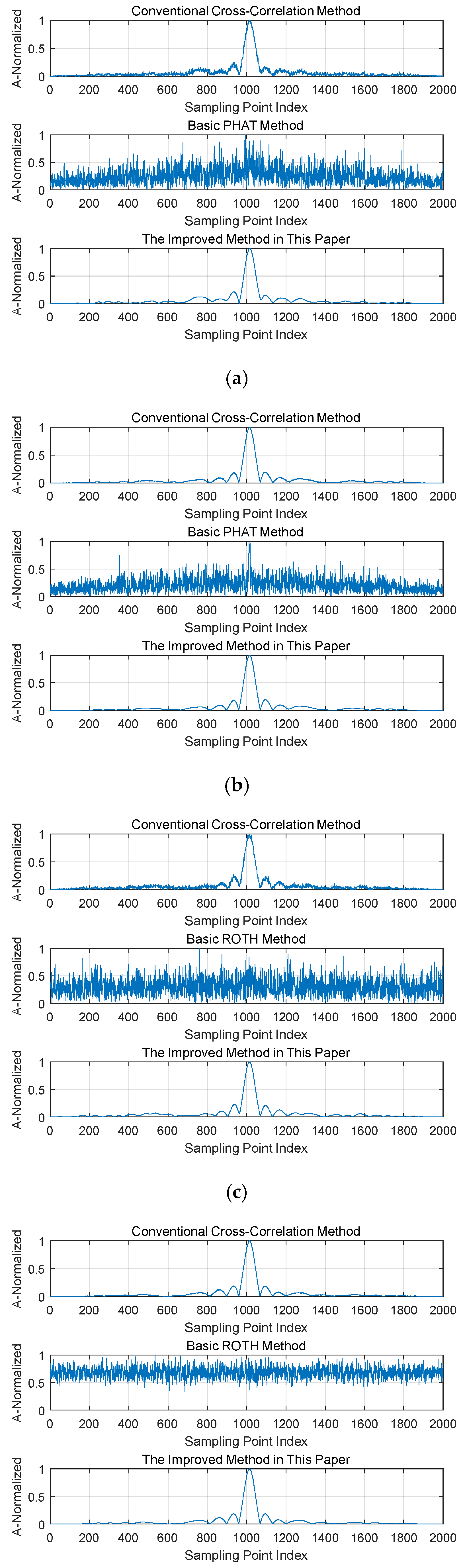
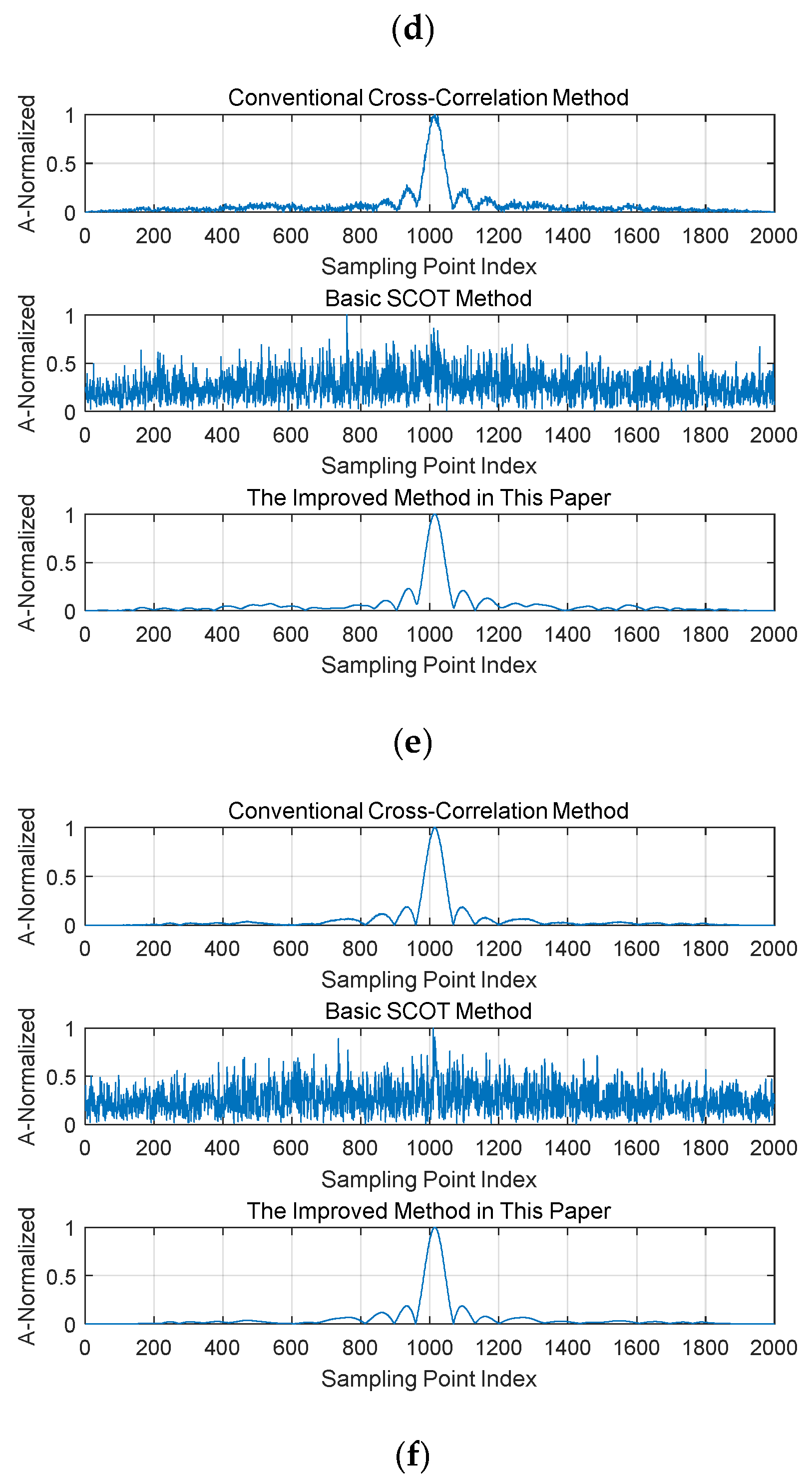
By comparing with the conventional cross-correlation function method, it can be observed that, in contrast to the original weighting function method, all improved weighting function methods can completely retain the pulse compression gain. Even under the low SNR condition of 0 dB, the peaks of the cross-correlation function are still clearly visible and exhibit a better SNR than those obtained by the conventional cross-correlation function method. This indicates that the improved weighting function methods can filter out the influence of most noise while protecting the effective frequency band of the signal. Therefore, it can be inferred that the improved frequency-domain weighting algorithm can achieve better coherent parameter estimation performance. In the following, the coherent parameter estimation performance of the improved weighting function method is simulated, and a comparative analysis is conducted with the basic generalized cross-correlation function method and the method proposed in Reference [17].
The simulation parameters remain unchanged, and 1,000 Monte Carlo simulation experiments are conducted. The simulation results are shown in the figure below. In the figure, the abscissa represents the SNR of the signal, and the ordinate represents either the time delay estimation accuracy (with the unit of ns) or the phase difference estimation accuracy (with the unit of °). The blue curve denotes the basic PHAT method, basic ROTH method, or basic SCOT method; the red curve represents the corresponding improved method from Reference [17]; the yellow curve stands for the corresponding improved method proposed in this paper; and the brown curve indicates the CRLB for CPs estimation.
By comparing the blue curves in Figure 6, Figure 7, and Figure 8, it can be observed that the time delay estimation error and phase difference estimation error of the basic PHAT method and the basic SCOT method are lower than those of the basic ROTH method. This is consistent with the results obtained from the CC function in Figure 8, and the reason has been explained in the previous text, so it will not be repeated here.
Figure 6.
Comparison of estimation performance of the PHAT method before and after improvement (a) Comparison of Time Delay Estimation Accuracy (b) Comparison of Phase Difference Estimation Accuracy.
Figure 6.
Comparison of estimation performance of the PHAT method before and after improvement (a) Comparison of Time Delay Estimation Accuracy (b) Comparison of Phase Difference Estimation Accuracy.
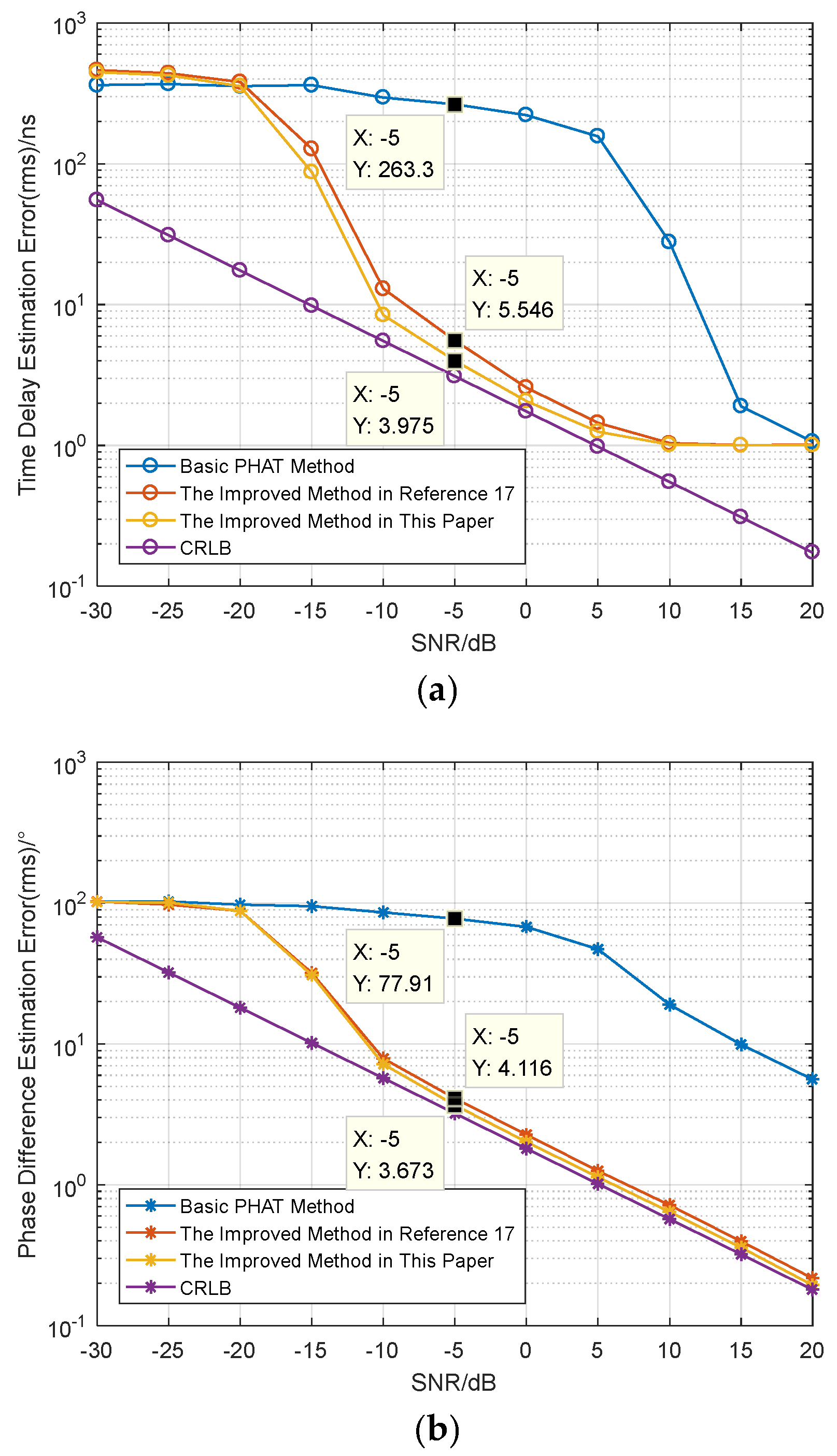
Figure 7.
Comparison of estimation performance of the ROTH method before and after improvement (a) Comparison of Time Delay Estimation Accuracy (b) Comparison of Phase Difference Estimation Accuracy.
Figure 7.
Comparison of estimation performance of the ROTH method before and after improvement (a) Comparison of Time Delay Estimation Accuracy (b) Comparison of Phase Difference Estimation Accuracy.
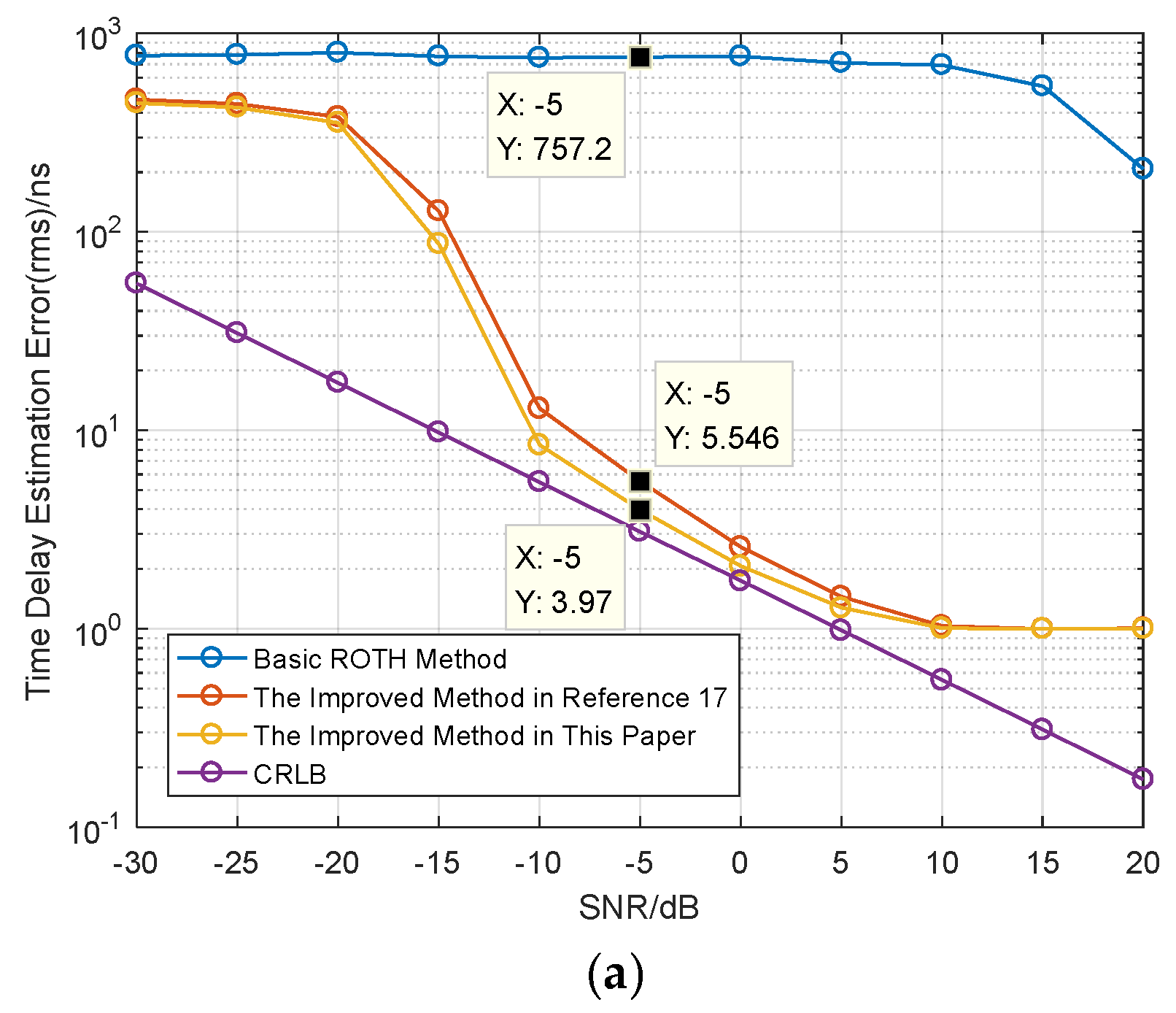
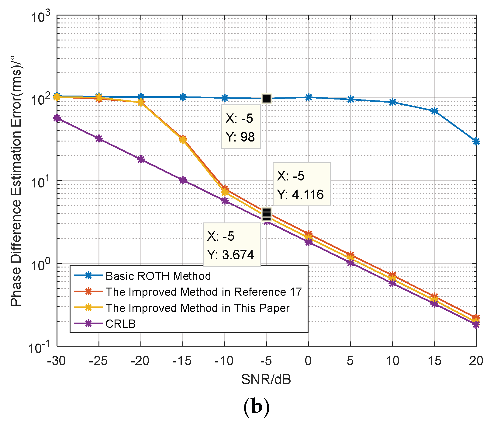
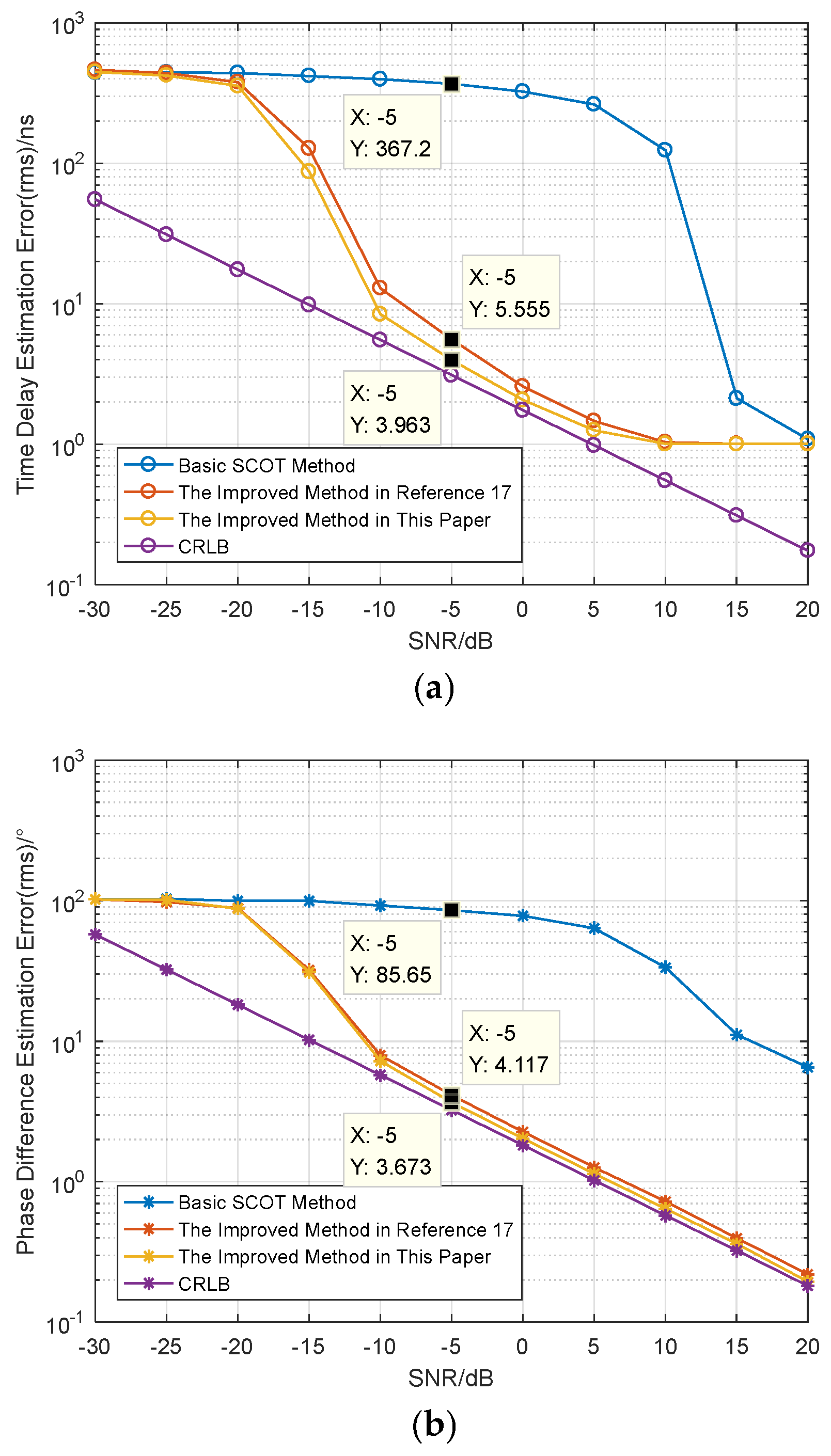
Figure 8.
Comparison of estimation performance of the SCOT method before and after improvement (a) Comparison of Time Delay Estimation Accuracy (b) Comparison of Phase Difference Estimation Accuracy.
Figure 8.
Comparison of estimation performance of the SCOT method before and after improvement (a) Comparison of Time Delay Estimation Accuracy (b) Comparison of Phase Difference Estimation Accuracy.
By comparing the red curve, yellow curve, and blue curve in Figure 6(a), it can be observed that the time delay estimation error of the PHAT-based improved method proposed in this paper is lower than that of the improved method from Reference [17] and the basic PHAT method. When the SNR is -5dB, the time delay estimation error of the PHAT-based improved method in this paper is 3.975ns, which is much lower than that of the basic PHAT method (with a time delay estimation error of 263.3ns). Compared with the improved method from Reference [17] (with a time delay estimation error of 5.546ns), the time delay estimation performance is improved by 28.3%, which verifies the effectiveness of the weighting function proposed in this paper for the PHAT method.
By comparing the red curve, yellow curve, and blue curve in Figure 6(b), it can be seen that the phase difference estimation error of the PHAT-based improved method in this paper is slightly lower than that of the improved method from Reference [17] and much lower than that of the basic PHAT method. When the SNR is -5dB, the phase difference estimation error of the PHAT-based improved method in this paper is 3.673°, which is far lower than that of the basic PHAT method (with a phase difference estimation error of 77.91°). Compared with the improved method from Reference [17] (with a phase difference estimation error of 4.116°), the phase difference estimation performance is improved by 10.8%.
By comparing the red curve, yellow curve, and blue curve in Figure 7(a), it can be observed that the time delay estimation error of the ROTH-based improved method proposed in this paper is lower than that of the improved method from Reference [17] and the basic ROTH method. When the SNR is -5dB, the time delay estimation error of the ROTH-based improved method in this paper is 3.97ns, which is much lower than that of the basic ROTH method (with a time delay estimation error of 757.2ns). Compared with the improved method from Reference [17] (with a time delay estimation error of 5.546ns), the time delay estimation performance is improved by 28.4%, which verifies the effectiveness of the weighting function proposed in this paper for the ROTH method.
By comparing the red curve, yellow curve, and blue curve in Figure 6(b), it can be seen that the phase difference estimation error of the ROTH-based improved method in this paper is slightly lower than that of the improved method from Reference [17] and much lower than that of the basic ROTH method. When the SNR is -5 dB, the phase difference estimation error of the ROTH-based improved method in this paper is 3.674°, which is far lower than that of the basic ROTH method (with a phase difference estimation error of 98°). Compared with the improved method from Reference [17] (with a phase difference estimation error of 4.116°), the phase difference estimation performance is improved by 10.7%.
By comparing the red curve, yellow curve, and blue curve in Figure 8(a), it can be observed that the time delay estimation error of the SCOT-based improved method proposed in this paper is lower than that of the improved method from Reference [17] and the basic SCOT method. When the SNR is -5dB, the time delay estimation error of the SCOT-based improved method in this paper is 3.963ns, which is much lower than that of the basic SCOT method (with a time delay estimation error of 367.2ns). Compared with the improved method from Reference [17] (with a time delay estimation error of 5.56ns), the time delay estimation performance is improved by 28.7%, which verifies the effectiveness of the weighting function proposed in this paper for the SCOT method.
By comparing the red curve, yellow curve, and blue curve in Figure 6(b), it can be seen that the phase difference estimation error of the SCOT-based improved method in this paper is slightly lower than that of the improved method from Reference [17] and much lower than that of the basic SCOT method. When the SNR is -5dB, the phase difference estimation error of the SCOT-based improved method in this paper is 3.673°, which is far lower than that of the basic SCOT method (with a phase difference estimation error of 85.65°). Compared with the improved method from Reference [17] (with a phase difference estimation error of 4.117°), the phase difference estimation performance is improved by 10.8%.
The statistical results of time delay estimation accuracy and phase difference estimation error of the improved methods based on the PHAT method, ROTH method, and SCOT method in this paper under different SNR are shown in the table below, where each data in the table retains four significant figures.
As evident from Table 1, for estimating time delay and phase difference, the estimation errors remain largely consistent across various SNRs, despite employing different weighting methods. This consistency arises because, in the scenario addressed by this paper, the received signalsand from interference units share the same frequency spectrum, and the noise is independently and identically distributed (i.i.d.). Consequently, irrespective of the normalization technique applied, the denominator term of the weighting function remains the same when noise effects are disregarded, equating to the amplitude of the signal’s auto-power spectrum. Frequency-domain protection processing eliminates the impact of most noise frequency bands. Consequently, the resulting auto-correlation function not only maximally attenuates the noise but also preserves the pulse compression gain of the original signal. Hence, the enhanced frequency-domain weighting method proposed in this paper represents a more fundamental form of generalized correlation processing.
4. Conclusions
Addressing the core issue of coherent parameter estimation for distributed coherent jamming systems, this paper begins with the operational workflow of such systems and presents a corresponding signal model. Considering time synchronization errors and phase synchronization errors, the paper derives the CRLB for the estimation of coherent parameters, (including time delay and phase difference, providing theoretical guidance for engineering implementation. Combined with practical engineering application scenarios, the theoretical feasibility of the distributed coherent jamming system is analyzed. Based on the implementation process of the system, it is pointed out that the primary factors affecting time synchronization accuracy and phase synchronization accuracy are the short-term frequency stability of the frequency source—this insight offers a theoretical basis for the engineering implementation of high-precision coherent parameter estimation in distributed systems.
Regarding the problem of coherent parameter estimation methods, the paper analyzes the cross-correlation function characteristics and amplitude-phase characteristics of cross-power spectra for four methods: the cross-correlation function method, PHAT method, ROTH method, and SCOT method. It identifies the limitations of these existing methods and proposes a time delay and phase difference estimation method based on frequency-domain threshold processing. This proposed method preserves the effective frequency band of the signal and performs noise whitening through frequency-domain thresholding, thereby fully preserving the pulse compression gain of the signal while suppressing noise.
The proposed method is applied to the PHAT, ROTH, and SCOT methods respectively. Monte Carlo simulation results demonstrate that the coherent parameter estimation accuracy of all three methods is significantly improved after integrating the proposed method: Compared with the basic PHAT generalized cross-correlation method, the time delay estimation accuracy is improved by 28.3%, and the phase difference estimation accuracy is improved by 10.8%. Compared with the basic ROTH generalized cross-correlation method, the time delay estimation accuracy is improved by 28.4%, and the phase difference estimation accuracy is improved by 10.7%. Compared with the basic SCOT generalized cross-correlation method, the time delay estimation accuracy is improved by 28.7%, and the phase difference estimation accuracy is improved by 10.8%. Both theoretical analysis and simulation results confirm that the method proposed in this paper is a more fundamental generalized correlation algorithm.
Funding
Not applicable.
Institutional Review Board Statement
Not applicable.
Informed Consent Statement
Not applicable.
Data Availability Statement
Data are contained within the article.
Conflicts of Interest
The authors declare no conflicts of interest.
References
- LIU, Xinghua; WANG, Guoyu; XU, Zhenhai; et al. Review of principles, development and technical implementation of coherently combining distributed apertures[J]. Journal of Radars 2023, 12(6), 1229–1248. [Google Scholar]
- LIU, Quanhua; ZHANG, Kaixiang; LIANG, Zhennan; et al. Research overview of ground-based distributed coherent aperture radar.
- [J]. Journal of Signal Processing 2022, 38(12), 2443–2459.
- YIN, Pilei. Research on Ground-Based Wideband Distributed Coherent Aperture Radar[D]; Beijing Institute of Technology, 2016. [Google Scholar]
- ZHANG, Honggang; LEI, Zijian; LIU, Quanhua. Coherent Parameters Estimation Method Based on MUSIC in Wide-band Distributed Coherent Aperture Radar[J]. Journal of Signal Processing 2015, 31(2), 208–214. [Google Scholar]
- SONG, Jing; ZHANG, Jianyun; DAI, Lin; et al. Parameter estimation and coherence performance of distribute daperture coherent radar based on phase synchronization[J]. Science China: information science.
- YIN, Pilei; ZHANG, Honggang; ZHAI, Tengpu; et al. Coherent Parameters Estimation Using Kalman Filter in Distributed Coherent Aperture Radar[J]. Transactions of Beijing Institute of Technology 2016, 36(3), 282–288. [Google Scholar]
- LIU, Tianxiang; HUANG, Pan; JIANG, Yansong; et al. Parameter Estimation Method for Wideband Distributed Coherent Radar by Combining Multi-pulse Accumulation with CAPON Algorithm[J]. Modern Radar 2025, 1–9. Available online: http://kns.cnki.net/kcms/detail/32.1353.tn.20250326.1538.002.html.
- CHEN, Qiuju; JIANG, Qiuxi; ZENG, Fangling; et al. Single frequency spatial power combining using sparse array based on time reversal of electromagnetic wave[J]. Acta Phys. Sin. 2015, 64(20), 204101. [Google Scholar]
- CHEN, Qiuju; JIANG, Qiuxi; ZENG, Fangling; et al. Spatial power combining of time reversal pulse signal using sparse array[J]. Chinese journal of radio science 2016, 31(3), 553–561. [Google Scholar]
- TIAN, Siyuan. Research on Spatial Power Combination Technology of Distributed Array Based on Time Reversal[M]; Graduate School of National University of Defense Technology, 2019. [Google Scholar]
- TIAN, Siyuan; CHEN, Qiuju; HUANG, Jianchong; et al. Research on Far-Field Power Synthesis of Moving Array Based on Time Inversion Technology[J]. Journal of Air Force Engineering University(Natural Science Edition) 2020, 21(1), 58–63. [Google Scholar]
- TIAN, Siyuan; HUANG, Jianchong; CHEN, Qiuju; et al. Application of time reversal technology in electronic countermeasure and the trend analysis[J]. Electronic Optics & Control 2020, 27(4), 55–60. [Google Scholar]
- JU, Tao; HUANG, Gaoming; MAN, Xin. Model and Efficiency Analysis of Spatial Power Combining on Distributed Jamming Devices[J]. Ship Electronic Engineering 2020, 27(4), 148–151. [Google Scholar]
- LU, Shiyuan; JIANG, Chunshan; ZHOU, Yuanming. Application Analysis of Distributed Power Synthesis Technology in Electronic Warfare Equipment[J]. Joumal of CAEIT 2020, 15(9), 861–865+871. [Google Scholar]
- JU, Tao; HUANG, Gaoming; MAN, Xin. A Spatial Power Synthetic Method for Random Distributed Array Communication Jammers[J]. Fire Control& Command Control 2020, 45(8), 57–61+67. [Google Scholar]
- XING, Yuhua; WANG, Heng. Optimization of Time Delay Estimation by Singular Spectral Decomposition and Improved Generalized Correlation Method[J]. Advances in Laser and Optoelectronics 2024, 61(5), 0506008-1-9. [Google Scholar]
- GUAN, Yu; DONG, Ming; CHANG, Haoxin; et al. Partial Discharge Ultrasound Location Method Based on SRLMSGCC Algorithm[J]. Power System Technology 2025, 49(4), 1708–1716. [Google Scholar]
- TANG, Xiaowei. Research on Key Issues in Distributed Coherent Radar[D]; Tsinghua University, 2013. [Google Scholar]
- XU, Ruiqi; WEI, Wei; XIE, Weilin; et al. Coherent Combination of Multi-channel Signals Based on High-precision Time-frequency Difference Estimation[J]. Optical Technique 2025, 51(1), 66–71. [Google Scholar]
- WANG, Nan; LUO, Yongjiang1; YANG, Jiali; et al. Wireless frequency fynchronization method for distributed coherent aperture radar in complex environments[J]. Systems Engineering and Electronics. Available online: https://link.cnki.net/urlid/11.2422.TN.20250325.2120.010.
- ZHANG, Yubo; GAO, Jian; WANG, Rentao. A Time Synchronization Scheme for Ground-based Distributed Coherent Aperture Radar[J]. Fire Control Radar Technology 2025, 54(1), 94–98. [Google Scholar]
- ZHOU, Lisha; LIN, Baojun; SHAORuiqiang; et al. BeiDOU-3 Satellite autonomous Time Synchronization Algorithm for Clock Jumps[J]. Journal of National University of Defense Technology 2025, 47(1), 222–229. [Google Scholar]
- ZHANG, Na; GUO, Fang; JIANG, Xianfeng; et al. The Research of Phase Noise and Frequency Stability in Time Frequency Signal[J]. Annals of Shanghai Astronomical Observatory 2009, (00), 146–152. [Google Scholar]
- XIAO, Jiangning; SHANG, Junna; HUO, Gang. Time Difference Estimation Algorithm Based on VDM and Generalized Extended Approximation[J]. Chinese Journal of Sensors and Actuators 2025, 38(3), 468–476. [Google Scholar]
- SUN, Jianhao; JIAN, Genshan; ZHANG, Wei; et al. Research on high-precision multipath delay estimation based on phase compensation[J]. Chinese Journal of Scientific Instrument 2024, 45(8), 307–315. [Google Scholar]
- CHEN, Haihong; YI, Yongli; HAN, Yu; et al. Power Noise Source Location Algorithm Based on Frequency Sliding Generalized Cross-Correlation[J]. Technical Acoustics 2024, 43(4), 550–556. [Google Scholar]
- ZHANG, Zeyu; TANG, Xiaojun; LI, Xiaobin; et al. Partial Discharge Localization based on Hybrid TDOA/DOA with Blind Signal Separation Algorithm[J]. Acta Physica Sinica. Available online: https://link.cnki.net/urlid/11.1958.o4.20250510.2117.002.
- WEI, Jiechang; ZHENG, Weimin; Tong, Li. Simulation of VLBI Digtial Baseband Signal with Time Delay[J]. Annals of Shanghai Astronomical Observatory 2015, (00), 124–135. [Google Scholar]
Figure 1.
Schematic Diagram of the Spatial Positions of Jamming Units and the Radar Target.
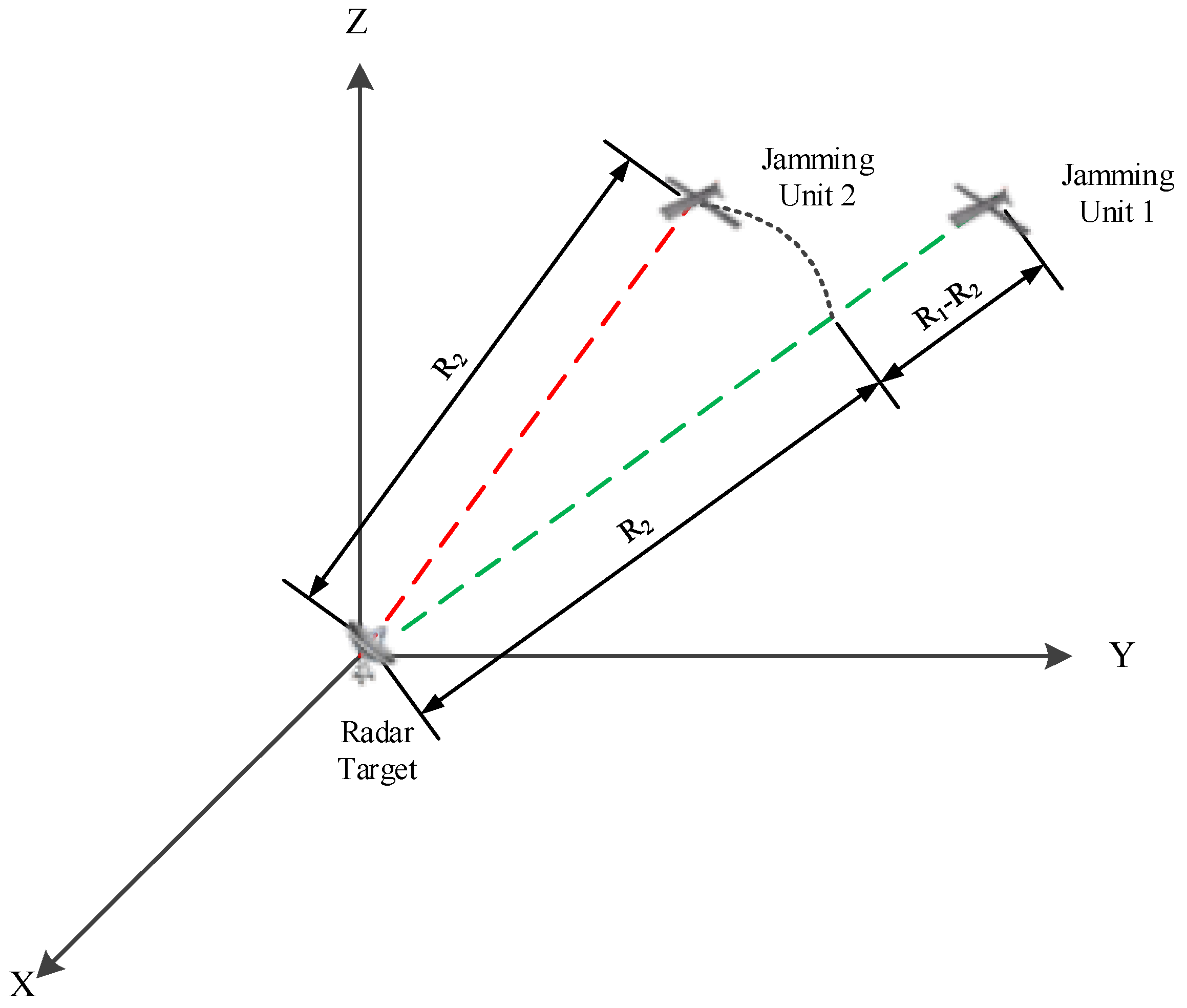

Table 1.
Statistical Table of CPs Estimation Errors of The Improved Weighting Method in this Paper under Different SNRs.
Table 1.
Statistical Table of CPs Estimation Errors of The Improved Weighting Method in this Paper under Different SNRs.
| Time Delay Estimation Error (ns) | Phase Difference Estimation Error (°) | |||||
|---|---|---|---|---|---|---|
| SNR | Based on the PHAT Method | Based on the ROTH Method | Based on the SCOT Method | Based on the PHAT Method | Based on the ROTH Method | Based on the SCOT Method |
| -30 | 446.0 | 446.0 | 446.0 | 102.3 | 102.3 | 102.3 |
| -25 | 423.3 | 423.3 | 423.3 | 101.0 | 101.0 | 101.0 |
| -20 | 355.6 | 355.3 | 355.6 | 87.97 | 87.97 | 87.98 |
| -15 | 87.11 | 87.12 | 87.11 | 31.02 | 31.02 | 31.02 |
| -10 | 8.417 | 8.427 | 8.411 | 7.209 | 7.208 | 7.208 |
| -5 | 3.975 | 3.970 | 3.963 | 3.673 | 3.674 | 3.674 |
| 0 | 2.062 | 2.068 | 2.062 | 2.030 | 2.030 | 2.030 |
| 5 | 1.252 | 1.275 | 1.255 | 1.139 | 1.139 | 1.138 |
| 10 | 1.009 | 1.009 | 1.005 | 0.6418 | 0.6414 | 0.6415 |
| 15 | 1.002 | 1.002 | 1.002 | 0.3587 | 0.3584 | 0.3588 |
| 20 | 1.004 | 1.005 | 1.005 | 0.1944 | 0.1946 | 0.1945 |
Disclaimer/Publisher’s Note: The statements, opinions and data contained in all publications are solely those of the individual author(s) and contributor(s) and not of MDPI and/or the editor(s). MDPI and/or the editor(s) disclaim responsibility for any injury to people or property resulting from any ideas, methods, instructions or products referred to in the content. |
© 2026 by the authors. Licensee MDPI, Basel, Switzerland. This article is an open access article distributed under the terms and conditions of the Creative Commons Attribution (CC BY) license (http://creativecommons.org/licenses/by/4.0/).
Copyright: This open access article is published under a Creative Commons CC BY 4.0 license, which permit the free download, distribution, and reuse, provided that the author and preprint are cited in any reuse.


