Submitted:
05 February 2026
Posted:
06 February 2026
You are already at the latest version
Abstract
Abandoned oil and gas wells pose significant risks to human health and the environment by emitting air pollutants, contaminating groundwater, and leaving behind hazardous debris. In the United States, approximately 3.9 million documented wells vary widely in the accuracy of their recorded locations and plugging status, creating major challenges for detection, mapping, and remediation. Existing methods show some promise but often lose effectiveness under complex conditions, such as vegetation occlusion or construction without metal components.
In this study, we propose a drone-based approach equipped with a highly sensitive methane sensor to detect elevated methane concentrations. To address the noisy and variable nature of environmental sensor data, statistical methods were developed that enable reliable detection of low-level emissions under field conditions. Controlled release experiments with known emission points validated the method’s ability to localize candidate sources. We further tested the approach at a field site containing three abandoned wells with known locations and sparse emission profiles. The results demonstrate that the proposed drone-based sensing method provides a scalable, cost-effective solution for the high-confidence identification of actively leaking wells and offers a direct indicator of environmental risk, supporting targeted monitoring and the prioritization of remediation efforts.
Keywords:
abandoned wells
; methane
; drones
; oil and gas
; laser gas detector
1. Introduction
The oil and gas (O&G) industry has operated in the US for over 200 years, yet not until the Clean Air Act of 1963 did environmental protection begin to be legislated and enforced. According to the United States Environmental Protection Agency’s report on the Inventory of Greenhouse Gas Emissions and Sinks in 2024, there are about 3 million abandoned wells nationwide [1]. An ‘abandoned’ well is a well no longer in production, has a legally responsible owner and can be either plugged or unplugged. In addition to abandoned wells, ‘orphaned’ wells are a category of unplugged, nonproducing wells with no legally responsible party [2]. As of 2023, the number of documented orphaned wells was 117,672 [3] and estimated number of undocumented orphaned wells was between 310,000 – 800,000 [4]. In this work, both abandoned and orphaned O&G wells are collectively referred to as abandoned O&G wells, recognizing that terminology may vary by state.
Research in the last 10 years has shown unplugged, abandoned O&G wells constitute a consistent pathway for Methane (CH4) to be fugitively released to the atmosphere and damage environmental/human health [5,6,7,8,9]. CH4 is a prominent greenhouse gas with a short atmospheric lifespan of ~10 years. Compared to carbon dioxide (CO2), another greenhouse gas, the global warming potential of CH4 over 20 years is 86 times greater. Due to its properties, CH4 has been targeted by many climate change mitigation initiatives as benefits from reductions would be realized sooner than reducing CO2 would. CH4 is emitted naturally as a part of the carbon cycle and anthropogenically from three main industries: Oil and Gas (O&G), Solid Waste Management, and Agricultural. Among these anthropogenic sources, the US Oil & Gas (O&G) industry accounts for ~ 30-40% of its country’s CH4 emissions [10] The US EPA estimates a quantity of CH4 of 282 million tons of CO2 equivalent with abandoned wells contributing 8.5 million tons of CO2 equivalent or about 3% of the sector’s total CH4 emissions [1]. It is worth noting the considerable uncertainty present in these estimates, relative to millions of abandoned wells only 1125 wells, <0.03 of total abandoned wells, have had their emissions measured [11]. In addition to the climate risk from CH4 emissions, abandoned wells present risks to human and environmental health. Unplugged wells provide a pathway for remaining oil or gas to migrate to the surface and contaminate ground and surface water resources. Benzene, a known carcinogen, can be expected to be co-emitted with CH4, a study of wells in Pennsylvania detected benzene at 70% of sites. The buildup of CH4 in an enclosed space can lead to dangerous explosions when the lower explosive limit is reached [12]. When left improperly remediated, plugged or unplugged wells also pose a risk to areas where the land use has changed. For example, Oil Creek State Park is an area where abandoned wells have been studied and is now open to the public as a recreation area [13]. Deteriorated O&G infrastructure could injure those visiting the area.
With the risks documented, Section 40601, Title IV of the 2021 Bipartisan Infrastructure Law (BIL) made $4.675 billion of federal funds available for plugging, remediation, and restoration of orphaned well sites. Majority ($4.275 billion) of these funds were for the 28 states with documented abandoned wells they have assumed responsibility. The number of documented abandoned wells in each state determines the portion of funds received by state agencies. In Alaska, twelve documented abandoned wells have equated to $28,346,487 received in two phases of grants, the first in 2024 and the second in 2025 [14]. However, of the combined 3.9 million abandoned wells, characteristics vary and have meaningful effects on the environmental risks as well as remediation strategies. Well age, integrity, depth and plugging status have all been found to be correlated with greater CH4 emissions [15].
Methods to locate abandoned wells have largely been limited to aerial magnetometry surveys [6,13,16,17]. By detecting the magnetic anomalies created by steel well casings, these surveys have demonstrated the capabilities of the sensor but noted shortcomings related to measurement noise [17] and false positives caused by background magnetic anomalies [13]. A handheld Laser CH4 sensor using Tunable Diode Laser Absorption Spectroscopy (TDLAS) was used to verify leaks from abandoned wells on the ground in a prior work [8] and the technology has been used by the O&G and solid waste industry for leak detection and repair (LDAR) for at least 20 years [18]. Recent studies, coinciding with the proliferation of drone usage, have studied the use of drone mounted TDLAS sensors to detect CH4 emissions in landfill, permafrost, and gas pipeline contexts [19,20,21]. Another study of a TDLAS-drone combo system tested the system at Methane Emissions Technology Evaluation Center (METEC), a CH4 detection technology testing center operated by Colorado State University. By leaking natural gas from (~85% CH4) from wellheads, tanks, and separators, it was shown surveys with no CH4 leaks would have a roughly normal distribution of measurements whereas the distribution would be skewed if there was a methane leak. A skewness threshold separated the leak from no-leak scenarios with zero false positives or false negatives [22]. With the demonstrated effectiveness of drone-mounted TDLAS CH4 sensors to remotely detect CH4 leaks, this work will examine the ability of the systems to identify abandoned gas wells and monitor remediation activities.
2. Materials and Methods
2.1. Methane Collection System
The methane survey system comprised a Matrice 300 RTK (M300 RTK) drone platform, a statically mounted CH4 detection sensor, a lightweight onboard computer, and a specialized UgCS software (Figure 1). The M300 RTK is a quadrotor drone powered by two 12S lithium polymer (LiPo) batteries which provide up to 55 minutes of flight time without payload. An UgCS Skyhub served as the onboard computer to communicate between the drone, methane sensor, and the UgCS software from the ground control station. It also logged data, synchronized GNSS coordinates of drone locations with CH4 measurements, uploaded flight routes and allowed direct drone control via UgCS software.
CH4 detection was performed by using a Pergam Laser Falcon, a tunable diode-laser absorption spectroscopy (TDLAS) CH4 sensor capable of measuring CH4 column density within a range of 0 – 50,000 parts-per-million-per-meter (ppm⋅m) with an accuracy of ± 10% of the measured value. This high CH4 sensitivity is crucial to the proposed methodology, as methane emissions in the field are typically sparse and intermittent. The Laser Falcon operates by emitting infrared laser light at a wavelength of 1.653 µm [21], which is only absorbed by CH4 but not by CO2 or water vapor. The Laser Falcon was powered by an independent 3-cell 11.1V LiPo battery. With the added payload, the M300 RTK’s flight time was reduced to approximately 35 minutes, and variable wind conditions could further shorten operational duration.
For each field site, a pre-mission site visit was conducted to assess the area, determine a safe flight altitude, and identify potential obstacles for the drone. Because the methane surveys benefit from flying at the lowest possible altitude to maximize the likelihood of detecting emissions before they disperse, careful measurement of obstacle heights is critical for flight safety. A rangefinder, commonly used in forestry, utility and construction, was employed for this purpose.
The collected information was used to define the flight boundaries and create mission plans for grid-based area scans. The spacing between flight passes and the selected flight speed were determined based on the sensor’s field of view at a given altitude and its data acquisition rate. These parameters ensured approximately one CH4 measurement every meter and provided a sufficient dense grid to cover the area of interest. Whenever possible, the best practice is to design flight areas to be completed within a single flight. However, the UgCS software enabled route interruptions for battery replacement and can resume the mission from a designated waypoint if needed.
On-site surveys began with additional safety checks on obstacle heights and stability of attached payloads. Prior to take-off, wind speed and direction were recorded for later use before completing a pre-mission safety checklist. Due to the attached payloads, downward-facing obstacle avoidance sensors were deactivated. The M300 RTK has capability to automatically take-off and land but without downward sensors, it would use positioning based on GNSS locating and publicly available elevation models. To ensure safety of equipment and operators, manual take-off, taxiing, and landing are preferred when using the system. Once in the air, a controller responsiveness check was completed and then the survey could begin. Following the manual landing, collected data was downloaded off the on-board computer to begin the analysis process.
2.2. Pre-Processing
Laser path length during surveys with a TDLAS sensor is an important consideration when processing data as CH4 measures are collected as ppm*m. Previous work with TDLAS sensors to detect CH4 [21], found potential laser path length variations caused by non-linear drone movements and unaccounted for ground variations are main sources of uncertainty when using these sensors. For statically mounted sensors, an unexpected roll, tilt, or yaw will move the sensor off nadir-view, thus increasing laser path length and could result in a false detection. If the background CH4 levels are significant, an increase in the path length would include more background CH4 in the recorded measure. As such, data preprocessing is necessary to remove measurements collected under conditions where path lengths are likely to change. The primary scenarios identified include takeoff, taxiing, landing, and turns. As the drone adjusts its velocity when entering, existing or executing turns, the sensor may be displaced from its nadir-view position. To minimize the impact of these deviations, data collected during taxiing, takeoff, and landing were excluded using timestamps aligned with the recorded start and end times of each flight. Similarly, during stops and turns between flight paths, the drone slows down to complete the maneuver; therefore, a velocity threshold was identified and applied to filter out measurements obtained during the turns.
2.3. Skewness Analysis
Skewness serves as an effective statistical measure for distinguishing leak from no-leak scenarios based on the probability density distribution of CH4 measurements [22]. In no-leak scenarios, histograms of CH4 measurements will tend towards a normal distribution, reflecting background methane levels with symmetric variation. In contrast, leak scenarios exhibit positive skewness, characterized by a long right tail in the distribution
This statistical measure is incorporated into the proposed methodology. The unbiased skewness of each histogram is calculated following Equation (1) provided by [23]:
A skewness threshold is then determined experimentally to distinguish between leak and no-leak scenarios.
2.4. Clustering Analysis
Although skewness shows promise for characterizing the data distribution, it is crucial to determine an appropriate threshold to distinguish leak from non-leak cases. This challenge arises because methane can occur naturally in the environment due to factors such as nearby wetlands, landfills, or similar conditions that emit methane into the atmosphere. To address this, we apply spatial autocorrelation analysis to further characterize leak cases, which are expected to likely exhibit spatial patterns that are statistically distinct from those of non-leak cases. Spatial autocorrelation quantifies the degree to which values observed at nearby locations are similar or dissimilar, providing a useful measure for identifying spatial patterns. When nearby locations exhibit similar values, positive spatial autocorrelation is present, and the distribution is characterized by the clustering of similar values; conversely, negative spatial autocorrelation indicates that nearby locations tend to have dissimilar values [24]. Among the various measures of spatial autocorrelation, Moran’s I and Geary’s C are the most widely used, while Moran’s I is generally preferred due to its higher sensitivity, ease of interpretation, and consistency with other spatial statistics [24,25,26]. In this study, Global Moran’s I statistic, which provides a single summary value representing the overall degree of spatial autocorrelation, was employed. This measure is suitable for CH4 leak detection, as leak events are expected to produce spatially clustered high CH4 concentrations that differ significantly from the more dispersed background levels associated with nature sources such as wetlands, or landfills. Global Moran’s I is calculated using Equation 2 [27]:
where zi is the deviation of the value measure i from its mean (xi – ), wi,j is the spatial weight between feature i and j, N is equal to the total number of features, and S0 is the aggregate of all the spatial weights.
As with most statistical tests, the Moran’s I test begins with the formulation of a null hypothesis. For spatial pattern analysis, this null hypothesis is Complete Spatial Randomness (CSR). Which assumes that the observed spatial distribution of values is random and exhibits no spatial autocorrelation. In the context of methane detection, CSR implies that methane concentrations are spatially independent, with no clustering attributable to leak events. Along with the calculated Moran’s I, the test returns a z-score and a p-value, which indicates whether the null hypothesis can be rejected. The z-score represents the standardized value of the observed statistic relative to its expected value under CSR, expressed in terms of standard deviation. It is calculated as:
where E[I] is the expected normal distribution of I and V[I] is the variance of I. The p-value represents the probability that the observed spatial pattern could have arisen from a random process. A very small p-value indicates that such a pattern is highly likely to result from randomness, allowing us to reject the null hypothesis [28]. In leak cases, which are characterized by positive Moran’s I value, we expect the corresponding z-score and p-value to reveal statistically significant clustering of methane measurements, rather than a random spatial distribution. Accordingly, we reject the null hypothesis when these metrics indicate non-randomness. The z-scores and p-values used in this work are interpreted in accordance with the standard normal distributions (Figure 2).
The scale of spatial pattern analysis plays a critical role in Moran’s I calculation because it determines the neighborhood over which spatial relationships are evaluated. Mathematically, the scale affects the spatial weights matrix, which is used to calculate S0 and the corresponding Moran’s I values for each location. Two key parameters must be defined: the neighborhood size (spatial extent) and the mathematical weighting of observations within that neighborhood. An incremental spatial autocorrelation analysis was performed to determine the neighborhood size by identifying the distances that clustering was most significant in the data set. This was achieved by calculating I according to Eq. 2 at the minimum neighborhood distance, where a point only has one neighbor, and then increasing neighborhood distance incrementally [30]. The result of the process will be a plot comparing clustering significance and distance, from this plot a peak may be identified which can be interpreted as the distance at which clustering is most pronounced [31]. In the context of methane leak detection, this can be interpreted as the approximate size of a CH4 plume, that is, the distance over which elevated methane concentrations are spatially correlated.
The weighing scheme specifies how the influence of one location’s value diminishes with distance from another. Common approaches include:
- Inverse Distance (ID): Weight =1/d, where d is the distance between locations.
- Inverse Distance Squared (ID2): weight = 1/d2, giving strong emphasis to nearer neighbors.
- Fixed Distance (FD): weight = 1 for all locations within the neighborhood.
- Zone of Indifference (ZoI): Weight = 1 within the neighborhood and 1/d beyond it.
These parameter choices directly affect the sensitivity of Moran’s I to spatial patterns, and the optimal configuration should be determined experimentally for the specific application.
Results from both the skewness analysis and the clustering assessment using Global Moran’s I were combined to evaluate their agreement. A site was classified as a leak scenario when both skewness value and Moran’s I exceeded their respective thresholds.
3. Results and Discussion
3.1. Controlled Release
A series of controlled release tests were performed at a designated test site to validate the proposed methane detection methodology using the Methane Survey System. These tests were carried out at the University of Alaska Anchorage (UAA) Mat-Su campus in Palmer, Alaska, hereafter referred as Mat-Su site. This location was chosen due to its class G airspace classification and a large, unoccupied, and leveled lot on the north side of the property, which provided a safe and controlled environment for repeated drone flights.
To simulate a leaking well, methane was released at a constant rate of 0.8 liters per minute (LPM) using a 5% CH4 calibration gas mixture. The exact release location was recorded to compare with the detection results. A total of four flights were conducted over multiple dates: one baseline flight without methane release and three flights with the simulated leak. Each flight flew the same approximate 160m x 160m grid pattern, with 2m spacing between flight paths and a flight speed of 2m/s. Flights were conducted at varying altitudes to assess the impact of altitude on methane detection performance [20].The baseline control flight was conducted at 17m above ground level (AGL), while the three simulated leak flights were flown at altitude of 32m AGL, 20m AGL, and 25m AGL, respectively.
Preprocessing was applied to the raw measurement to remove erroneous measures associated with taxiing, takeoff, and landing by using timestamps aligned with the recorded survey start and end times. Furthermore, turning maneuvers were removed by filtering out all measurements below a velocity threshold of 1.8 m/s.
We implemented the proposed skewness analysis on the filtered CH4 measurements. Results showed surveys with a leak present have a noticeably higher skew. Test A with no leak present has a skewness of 1.41 compared to an average skewness of 9.61 from Tests B-C (Table 1).
Skewness results from the controlled release tests indicate a threshold of 1.5 is effective for distinguishing leak cases. This finding aligns well with the previously established threshold [22]. However, a higher threshold may be needed in field cases where either laser path length is more variable or elevated background CH4 levels are present. A more variable path length could lead to step changes in ppm-m measures which push skew higher. Elevated background CH4 levels will similarly affect skew if a CH4 source previously unaccounted for has spread into the test area.
Leak cases (Tests B-D) from the controlled release surveys were used to investigate the localization effect from the proposed hot spot analysis compared with the recorded release location. To determine the appropriate size of neighborhood for the hot spot analysis, Incremental Spatial Autocorrelation was used to find the peak z-score, which indicates the highest spatial autocorrelation at the corresponding neighborhood size (distance)(Figure 3). Clustering analysis is sensitive to how neighbors are identified when assessing spatial clustering. Using Test A point data, a comparison of conceptualization of distance methods was completed by calculating Global Moran’s I for each method at three different neighborhood distances. 1.18, 3, and 5 meters were chosen as the distance as they were the first three peaks from the Incremental Spatial Autocorrelation graph. The findings indicated ‘Zone of Indifference’ as the conceptualization of distance exhibits the most stable results across all cases for clustering analysis (Figure 4).
Results from Moran’s I indicates Tests B-D with statistically significant clustered pattern with an average z-score of 4.78, corresponding to a less than 1% chance the spatial clustered pattern was generated randomly (Table 1). Conversely, Test A without a leak present showed a pattern not significantly different from a random pattern. This statistical measure further validates the findings from skewness analysis. The agreement between Global Moran’s I and skew results indicates using both could act as 2-step verification process. However, the max skew value does not align with the max Moran’s I z-score demonstrating the sensitivity of each method. As skew does not consider the spatial distribution of measures, it is more sensitive to extreme outliers regardless of where they appear in relation to neighboring measures. Whereas Moran’s I consider outliers in relation to the nearby measures, the neighborhood is described by distance band and conceptualization of distance and will be more sensitive to clustering of higher measures. If a survey has a low skew, Global Moran’s I could still indicate significant clustering if the relative ‘high’ measure from the survey is near each other. This scenario would likely be indicative of a first-order effect at test and demonstrate methods should be used in conjunction to inform if a true leak case is present.
3.2. Field Site Verification
Three wells, located in Houston, Alaska, were selected for this study with the resources provided by the Alaska Oil and Gas Conservation Commission (AOGCC). They were identified in close proximity (Figure 5), enabling a single field survey site and allowing for in-situ verification of the proposed methodology. Additionally, according to the progress summary report conducted by an engineering consulting firm, Well 1 rose approximately 2 meters above the ground and is located closest to the highway. CH4 measurements taken from a photoionization detector (PID) indicated low levels of gas from outside the well casing, though exact leak rates were not provided. Well 2 is in the wooded area, buried approximately 0.5 meters below ground and was excavated to take PID measurements. These measures indicated active leaking from the well casing and water was also leaking from the casing. However, the exact leak rate was also not provided and the well itself was re-buried prior to this study. Well 3, also in the wooded area, was initially thought to be a water well and was excavated to identify it as a gas well. PID measures also indicated the well was leaking gas, though with no exact figure provided.
CH4-based detection methodology was tested in the field study area previously described. CH4 data was collected across three surveys: two conducted before remediation and one during the remediation process. Each survey included two flights: one at 25m AGL covering all three wells and another at 20m AGL focusing on Well 1, accounting for the presence of obstacles at the site
Additionally, the 25m AGL survey data was divided to reflect ground conditions: Wells 2 and 3 were located beneath tree cover, while Well 1 was situated in open ground. This division helped account for potential differences in methane dispersion due to canopy interference. However, the 25m AGL survey conducted during remediations was not divided as the site had been leveled and all vegetation obscuring the wells had been cleared (Table 2).
Figure 6.
Test E-H histograms of filtered ppm-m measures with test name, leak rate, skewness (S), and Z-score (Z) from Global Moran’s I superimposed.
Figure 6.
Test E-H histograms of filtered ppm-m measures with test name, leak rate, skewness (S), and Z-score (Z) from Global Moran’s I superimposed.
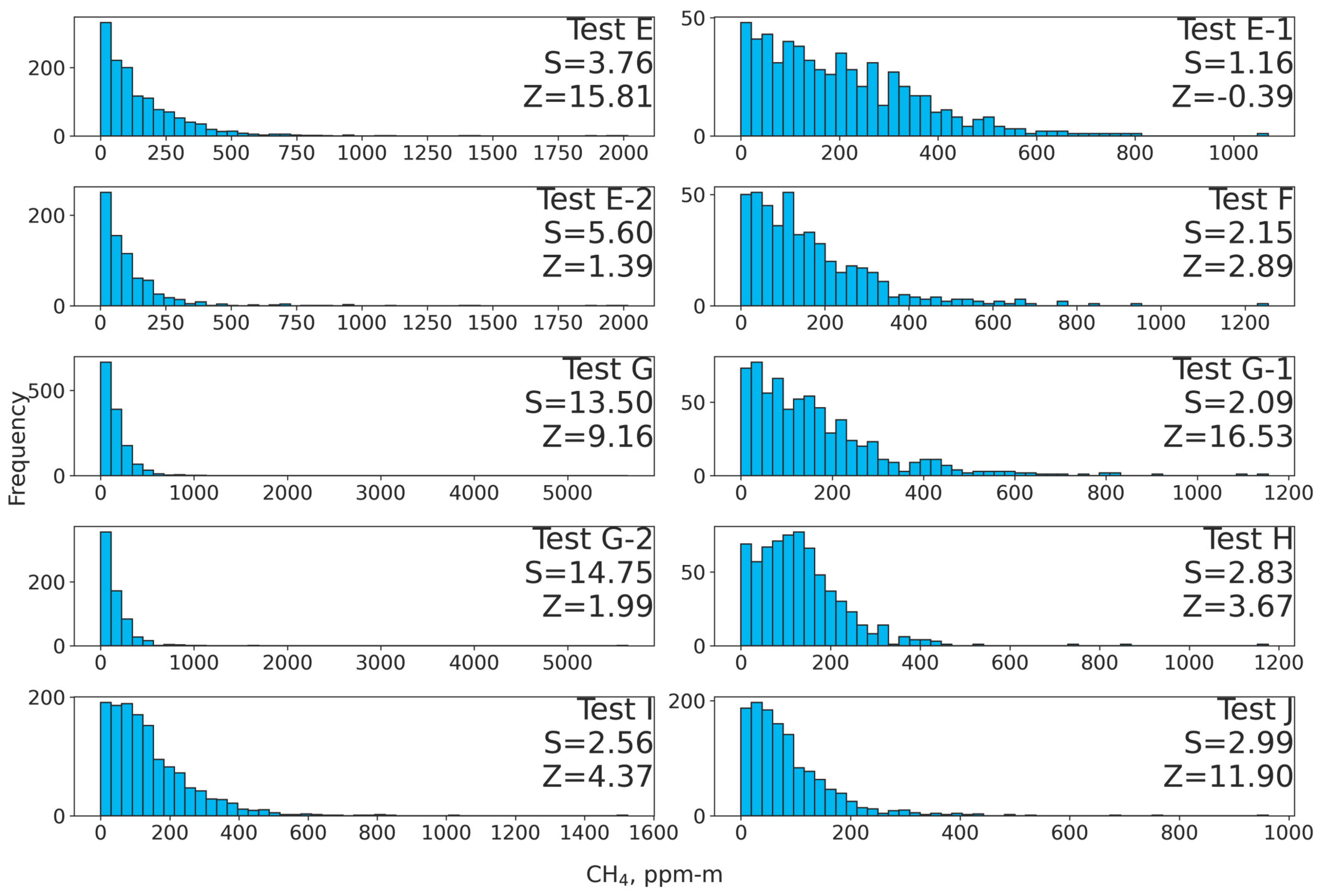
Test E & G covering Wells 1-3 both have skewness above the threshold of 1.5 and have z-scores indicating less than 1% likelihood the spatially clustered pattern is the result of random chance. The division data from Tests E & G also indicate there is a CH4 leak present, the results disagree over whether the leak is from Well 1 (Tests E-1, G-1) or Wells 2&3 (Tests E-2, G-2). Tests E-1 & E-2’s skewness, 1.16 and 5.60 respectively, indicate higher measurements originate from Wells 2&3 but neither Tests indicate statistically significant clustering. The Z-score for Test E-1 is negative but small, indicating there is no statistically significant pattern present. While E-2’s Moran’s I z-score is under the 1.65 threshold, a 1.39 z-score is still associated with only a 16% likelihood a pattern is the result of random chance. Tests G-1 & G-2’s skewness, 2.09 and 14.75 respectively, also indicate higher measurements originate from Wells 2&3, and both are above the 1.5 skewness threshold. Both G-1 and G-2 tests also indicate statistically significant clustering. The likelihood of clustering resulting from random chance is much lower for G-1 than G-2, indicated by their z-scores 16.53 and 1.99. Tests F & H indicate Well 1 is leaking, with both skewness above the 1.5 threshold, 2.15 and 2.83 respectively. Their Moran’s I z-scores indicate statistically significant clustering in both tests, 2.89 and 3.67 respectively.
Tests I & J indicate a leaking well is still present at the time of this survey. Skewness values from both tests are above the 1.5 threshold and Z-scores from Moran’s I indicate statistically significant clustering.
In summary, the skewness values indicate at least one well in the study area was emitting CH4 during all survey periods, both before and during remediation. The spatial clustering detected is statistically significant, further suggesting the presence of one or more wells of interest within the study area. Methane emissions in the area prior to remediation were further confirmed through site visits, as documented in the progress summary report provided by AOGCC.
3.3. Field Site Discussion
Field experiments demonstrate the effectiveness of the proposed methodology in identifying leak cases, which was further validated through third-party site visits. However, several important considerations should be pointed out. The skewness threshold of 1.5 was surpassed in every test except E-1. Z-scores from Moran’s I indicate statistically significant clustering in all but two surveys, E-1 & E-2. Notably, E-2 was only 6% below the 90% confidence threshold for clustering. As with the skewness results, the methane distribution in Test E-1 appeared random due to dynamic wind interference. Taken together, these findings strongly suggest there is at least one well leaking CH4 at the site, even during the remediation process. However, the disagreement between some Z-scores and skewness values highlight issues previously discussed, particularly the influence of wind conditions. As the site was located next to a busy highway, intermittent gust from passing cars would occasionally overpower the prevailing wind pattern measured prior to flight.
The effects of laser path length are also evident across the three surveys. Tests E&F took place after spring green-up had already occurred, Tests G&H took place after fall, and Test I&J took place after remediation work had cleared all vegetation cover and exposed the previously buried wells 2&3. Compared to the skewness of the full area Tests E and, skewness values decreased when isolating the unvegetated area around Well 1 (thus, a longer and more consistent laser path length), Tests E-1 and G-1, and increased when isolating the vegetated area around Wells 2 and 3 (thus, a variable and shorter laser path length), Tests E-2 and G-2. Despite those challenges, the skewness results are consistent with prior knowledge that Wells 2 and 3 were unplugged and leaking greater quantities of CH4. The effect of laser path length is more evident in the Moran’s I z-scores as inconsistencies in path length are more likely to reduce the number of possible elevated measures in a neighborhood. From summer to fall tests, Moran’s I z-scores increased in both divisions of the surveys (E and G). However, Moran’s I results from Tests E, E-1, and E-2 indicated dividing a completed survey in post-processing may remove important neighborhood context important to the Moran’s I algorithm, evidenced by the Z-score from Test E decreasing to below significance levels in Tests E-1 and E-2. Z-scores indicating statistical significance from the Tests I & J following the removal of vegetation also highlight the importance of a consistent laser path length for this methodology.
4. Conclusions
The combined skewness and clustering analysis was successful at identifying leak case scenarios both at the control and field site. Despite the encountered challenges related to atmospheric conditions and sensor laser path length, the statistical thresholds used are consistent with prior work, were confirmed using with the controlled CH4 release, and can be used in future CH4 leaking abandoned well detection. This methodology can be applied to additional CH4 LDAR tasks when a TDLAS CH4 sensor is used. Regardless of task, future surveys should design flight plans around key considerations discussed.
Future work should explore methods to detect abandoned wells which are not emitting CH4. For this subset of wells, methods could take advantage of additional well or well site characteristics. Such methods could also leverage deep learning techniques to lessen to overall amount of direct surveying which would be using traditional methods. While there has been recent work applying DL-based frameworks using CNNs as backbones to detect O&G infrastructure [32,33,34,35,36], few has been in the application of identifying abandoned oil and gas wells. For these frameworks to be successful, input data needs to be resilient to surface-level obstructions associated with well site deterioration, vegetation overgrowth, and varying terrain conditions.
Author Contributions
C.W. and W.H.T. designed the project; W.H.T. performed the experiments and analyzed the data; W.H.T. and C. W. evaluated and discussed the results of the experiments; W.H.T. wrote the paper; and C.W. finalized the manuscript writing, review and editing. All authors have read and agreed to the published version of the manuscript.
Funding
This research was funded by the National Science Foundation EPSCoR Cooperative Agreement OIA-2119689. Any opinions, findings, and conclusions or recommendations expressed in this material are those of the authors and do not necessarily reflect the views of the National Science Foundation.
Data Availability Statement
The data presented in this article are available on request from the corresponding author.
Acknowledgments
The authors acknowledge Alaska Oil & Gas Conservation Commission for experiment support.
Conflicts of Interest
The authors declare no conflicts of interest.
References
- U.S. Environmental Protection Agency. Inventory of U.S. Greenhouse Gas Emissions and Sinks: 1990-2022 – Main Text; 2024. https://www.epa.gov/ghgemissions/inventory-us-greenhouse-gas-emissions-and-.
- Boutot, J.; Peltz, A. S.; McVay, R.; Kang, M. Documented Orphaned Oil and Gas Wells Across the United States. Environ Sci Technol 2022, 56 (20), 14228–14236. [CrossRef]
- Merrill, M. D.; Grove, C. A.; Gianoutsos, N. J.; Freeman, P. A. Analysis of the United States Documented Unplugged Orphaned Oil and Gas Well Dataset; 2023.
- Interstate Oil and Gas Compact Commission (IOGCC). Idle and Orphan Oil and Gas Wells: State and Provincial Regulatory; 2021.
- Kang, M.; Christian, S.; Celia, M. A.; Mauzerall, D. L.; Bill, M.; Miller, A. R.; Chen, Y.; Conrad, M. E.; Darrah, T. H.; Jackson, R. B. Identification and Characterization of High Methane-Emitting Abandoned Oil and Gas Wells. Proc Natl Acad Sci U S A 2016, 113 (48), 13636–13641. [CrossRef]
- Pekney, N. J.; Diehl, J. R.; Ruehl, D.; Sams, J.; Veloski, G.; Patel, A.; Schmidt, C.; Card, T. Measurement of Methane Emissions from Abandoned Oil and Gas Wells in Hillman State Park, Pennsylvania. Carbon Manag 2018, 9 (2), 165–175. [CrossRef]
- Riddick, S. N.; Mbua, M.; Santos, A.; Emerson, E. W.; Cheptonui, F.; Houlihan, C.; Hodshire, A. L.; Anand, A.; Hartzell, W.; Zimmerle, D. J. Methane Emissions from Abandoned Oil and Gas Wells in Colorado. Science of the Total Environment 2024, 922. [CrossRef]
- Townsend-Small, A.; Ferrara, T. W.; Lyon, D. R.; Fries, A. E.; Lamb, B. K. Emissions of Coalbed and Natural Gas Methane from Abandoned Oil and Gas Wells in the United States. Geophys Res Lett 2016, 43 (5), 2283–2290. [CrossRef]
- Boothroyd, I. M.; Almond, S.; Qassim, S. M.; Worrall, F.; Davies, R. J. Fugitive Emissions of Methane from Abandoned, Decommissioned Oil and Gas Wells. Science of the Total Environment 2016, 547, 461–469. [CrossRef]
- Saunois, M.; R. Stavert, A.; Poulter, B.; Bousquet, P.; G. Canadell, J.; B. Jackson, R.; A. Raymond, P.; J. Dlugokencky, E.; Houweling, S.; K. Patra, P.; Ciais, P.; K. Arora, V.; Bastviken, D.; Bergamaschi, P.; R. Blake, D.; Brailsford, G.; Bruhwiler, L.; M. Carlson, K.; Carrol, M.; Castaldi, S.; Chandra, N.; Crevoisier, C.; M. Crill, P.; Covey, K.; L. Curry, C.; Etiope, G.; Frankenberg, C.; Gedney, N.; I. Hegglin, M.; Höglund-Isaksson, L.; Hugelius, G.; Ishizawa, M.; Ito, A.; Janssens-Maenhout, G.; M. Jensen, K.; Joos, F.; Kleinen, T.; B. Krummel, P.; L. Langenfelds, R.; G. Laruelle, G.; Liu, L.; MacHida, T.; Maksyutov, S.; C. McDonald, K.; McNorton, J.; A. Miller, P.; R. Melton, J.; Morino, I.; Müller, J.; Murguia-Flores, F.; Naik, V.; Niwa, Y.; Noce, S.; O’Doherty, S.; J. Parker, R.; Peng, C.; Peng, S.; P. Peters, G.; Prigent, C.; Prinn, R.; Ramonet, M.; Regnier, P.; J. Riley, W.; A. Rosentreter, J.; Segers, A.; J. Simpson, I.; Shi, H.; J. Smith, S.; Paul Steele, L.; F. Thornton, B.; Tian, H.; Tohjima, Y.; N. Tubiello, F.; Tsuruta, A.; Viovy, N.; Voulgarakis, A.; S. Weber, T.; Van Weele, M.; R. Van Der Werf, G.; F. Weiss, R.; Worthy, D.; Wunch, D.; Yin, Y.; Yoshida, Y.; Zhang, W.; Zhang, Z.; Zhao, Y.; Zheng, B.; Zhu, Q.; Zhu, Q.; Zhuang, Q. The Global Methane Budget 2000-2017. Earth Syst Sci Data 2020, 12 (3), 1561–1623. [CrossRef]
- Gianoutsos, N. J.; Haase, K. B.; Birdwell, J. E. Geologic Sources and Well Integrity Impact Methane Emissions from Orphaned and Abandoned Oil and Gas Wells. Science of the Total Environment. Elsevier B.V. February 20, 2024. [CrossRef]
- Kang, M.; Boutot, J.; McVay, R. C.; Roberts, K. A.; Jasechko, S.; Perrone, D.; Wen, T.; Lackey, G.; Raimi, D.; Digiulio, D. C.; Shonkoff, S. B. C.; William Carey, J.; Elliott, E. G.; Vorhees, D. J.; Peltz, A. S. Environmental Risks and Opportunities of Orphaned Oil and Gas Wells in the United States. Environmental Research Letters 2023, 18 (7). [CrossRef]
- Saint-Vincent, P. M. B.; Sams, J. I.; Reeder, M. D.; Mundia-Howe, M.; Veloski, G. A.; Pekney, N. J. Historic and Modern Approaches for Discovery of Abandoned Wells for Methane Emissions Mitigation in Oil Creek State Park, Pennsylvania. J Environ Manage 2021, 280. [CrossRef]
- Orphaned Wells Program Office. Orphaned Wells Program Annual Report to Congress; 2024. https://www.doi.gov/orphanedwells.
- Saint-Vincent, P. M. B.; Reeder, M. D.; Sams, J. I.; Pekney, N. J. An Analysis of Abandoned Oil Well Characteristics Affecting Methane Emissions Estimates in the Cherokee Platform in Eastern Oklahoma. Geophys Res Lett 2020, 47 (23). [CrossRef]
- Hammack, R.; Veloski, G.; Schlagenhauf, M.; Lowe, R.; Zorn, A.; Wylie, L. Using Drone-Mounted Geophysical Sensors to Map Legacy Oil and Gas Infrastructure; American Association of Petroleum Geologists AAPG/Datapages, 2020. [CrossRef]
- de Smet, T. S.; Nikulin, A.; Romanzo, N.; Graber, N.; Dietrich, C.; Puliaiev, A. Successful Application of Drone-Based Aeromagnetic Surveys to Locate Legacy Oil and Gas Wells in Cattaraugus County, New York. J Appl Geophy 2021, 186. [CrossRef]
- Buckley, S. G. Tunable Diode Lasers for Trace Gas Detection: Methods, Developments, and Future Outlook. Spectroscopy 2018, 33 (10), 26–29.
- Emran, B. J.; Tannant, D. D.; Najjaran, H. Low-Altitude Aerial Methane Concentration Mapping. Remote Sens (Basel) 2017, 9 (8). [CrossRef]
- Iwaszenko, S.; Kalisz, P.; Słota, M.; Rudzki, A. Detection of Natural Gas Leakages Using a Laser-Based Methane Sensor and Uav. Remote Sens (Basel) 2021, 13 (3), 1–16. [CrossRef]
- Oberle, F. K. J.; Gibbs, A. E.; Richmond, B. M.; Erikson, L. H.; Waldrop, M. P.; Swarzenski, P. W. Towards Determining Spatial Methane Distribution on Arctic Permafrost Bluffs with an Unmanned Aerial System. SN Appl Sci 2019, 1 (3). [CrossRef]
- Golston, L. M.; Aubut, N. F.; Frish, M. B.; Yang, S.; Talbot, R. W.; Gretencord, C.; McSpiritt, J.; Zondlo, M. A. Natural Gas Fugitive Leak Detection Using an Unmanned Aerial Vehicle: Localization and Quantification of Emission Rate. Atmosphere (Basel) 2018, 9 (9). [CrossRef]
- Zwillinger, D.; Kokoska, S. CRC Standard Probability and Statistics Tables and Formulae; CRC Press, 1999. [CrossRef]
- Chou, Y. H. Spatial Pattern and Spatial Autocorrelation. In Lecture Notes in Computer Science (Including Subseries Lecture Notes in Artificial Intelligence and Lecture Notes in Bioinformatics); 1995; Vol. 988, pp 365–376.
- Grekousis, G. Spatial Autocorrelation. In Spatial Analysis Methods and Practice: Describe – Explore – Explain through GIS; Cambridge University Press, 2020; pp 207–274. [CrossRef]
- Lin, J. Comparison of Moran’s I and Geary’s c in Multivariate Spatial Pattern Analysis. Geogr Anal 2023, 55 (4), 685–702. [CrossRef]
- Smith, M. J. De; Goodchild, M. F.; Longley, P. A. Geospatial Analysis: A Comprehensive Guide to Principles Techniques and Software Tools, Sixth.; Winchelsea Press: London, UK, 2018.
- Goodchild, M. F. Spatial Autocorrelation; Geo Books, 1986; Vol. Catmog 47.
- Mitchell, A. The ESRI Guide to GIS Analysis; ESRI Press, 2005; Vol. 2.
- Legendre, P.; Fortin, M. J. Spatial Pattern and Ecological Analysis. Vegetatio 1989, 80 (2), 107–138. [CrossRef]
- Ran, H.; Guo, Z.; Yi, L.; Xiao, X.; Zhang, L.; Hu, Z.; Li, C.; Zhang, Y. Pollution Characteristics and Source Identification of Soil Metal(Loid)s at an Abandoned Arsenic-Containing Mine, China. J Hazard Mater 2021, 413, 125382. [CrossRef]
- Wang, Z.; Bai, L.; Song, G.; Zhang, J.; Tao, J.; Mulvenna, M. D.; Bond, R. R.; Chen, L. An Oil Well Dataset Derived from Satellite-based Remote Sensing. Remote Sens (Basel) 2021, 13 (6). [CrossRef]
- Shi, P.; Jiang, Q.; Shi, C.; Xi, J.; Tao, G.; Zhang, S.; Zhang, Z.; Liu, B.; Gao, X.; Wu, Q. Oilwell Detection via Large-Scale and High-Resolution Remote Sensing Images Based on Improved YOLO V4. Remote Sens (Basel) 2021, 13 (16). [CrossRef]
- Ramachandran, N.; Irvin, J.; Omara, M.; Gautam, R.; Meisenhelder, K.; Rostami, E.; Sheng, H.; Ng, A. Y.; Jackson, R. B. Deep Learning for Detecting and Characterizing Oil and Gas Well Pads in Satellite Imagery. Nat Commun 2024, 15 (1). [CrossRef]
- Wu, H.; Dong, H.; Wang, Z.; Bai, L.; Huo, F.; Tao, J.; Chen, L. Semantic Segmentation of Oil Well Sites Using Sentinel-2 Imagery. In International Geoscience and Remote Sensing Symposium (IGARSS); Institute of Electrical and Electronics Engineers Inc., 2023; Vol. 2023-July, pp 6901–6904. [CrossRef]
- Zhang, Y.; Bai, L.; Wang, Z.; Fan, M.; Jurek-Loughrey, A.; Zhang, Y.; Zhang, Y.; Zhao, M.; Chen, L. Oil Well Detection under Occlusion in Remote Sensing Images Using the Improved YOLOv5 Model. Remote Sens (Basel) 2023, 15 (24). [CrossRef]
Figure 1.
Hardware components of the methane survey system, excluding the UgCS software.
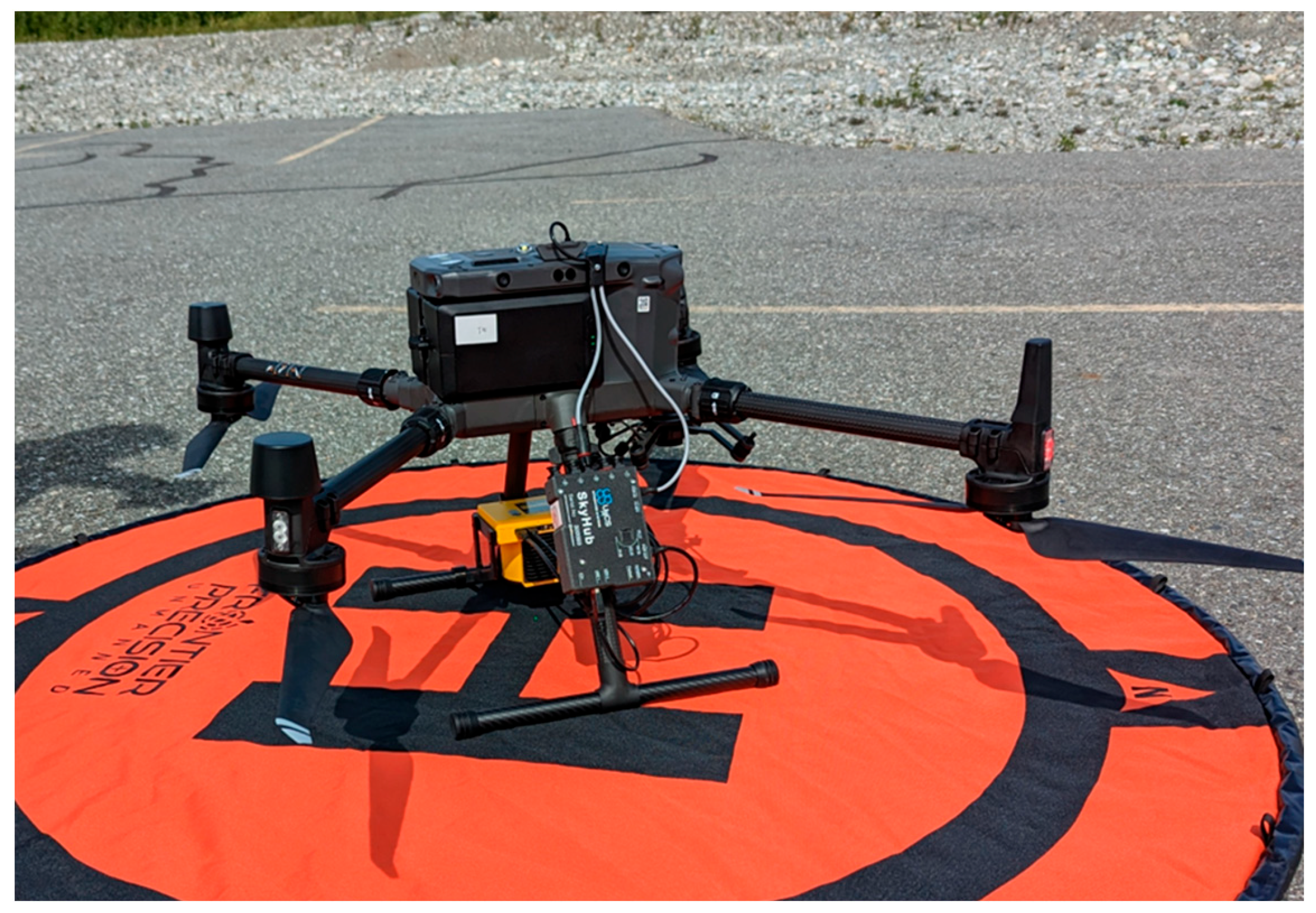
Figure 2.
Normal Distribution with 90, 95, and 99% confidence thresholds indicated [29].
Figure 2.
Normal Distribution with 90, 95, and 99% confidence thresholds indicated [29].
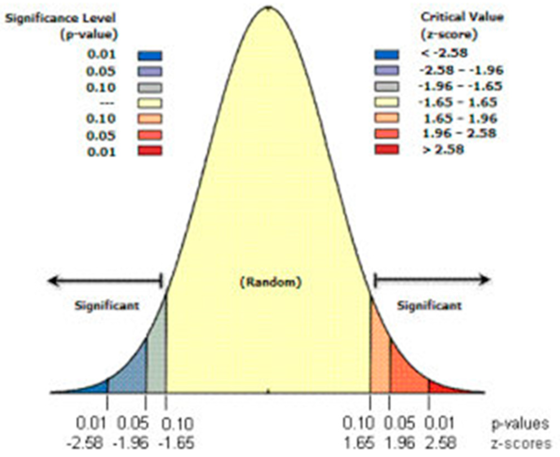
Figure 3.
Incremental Spatial Autocorrelation graph from Test B with max peak indicated at 3m.
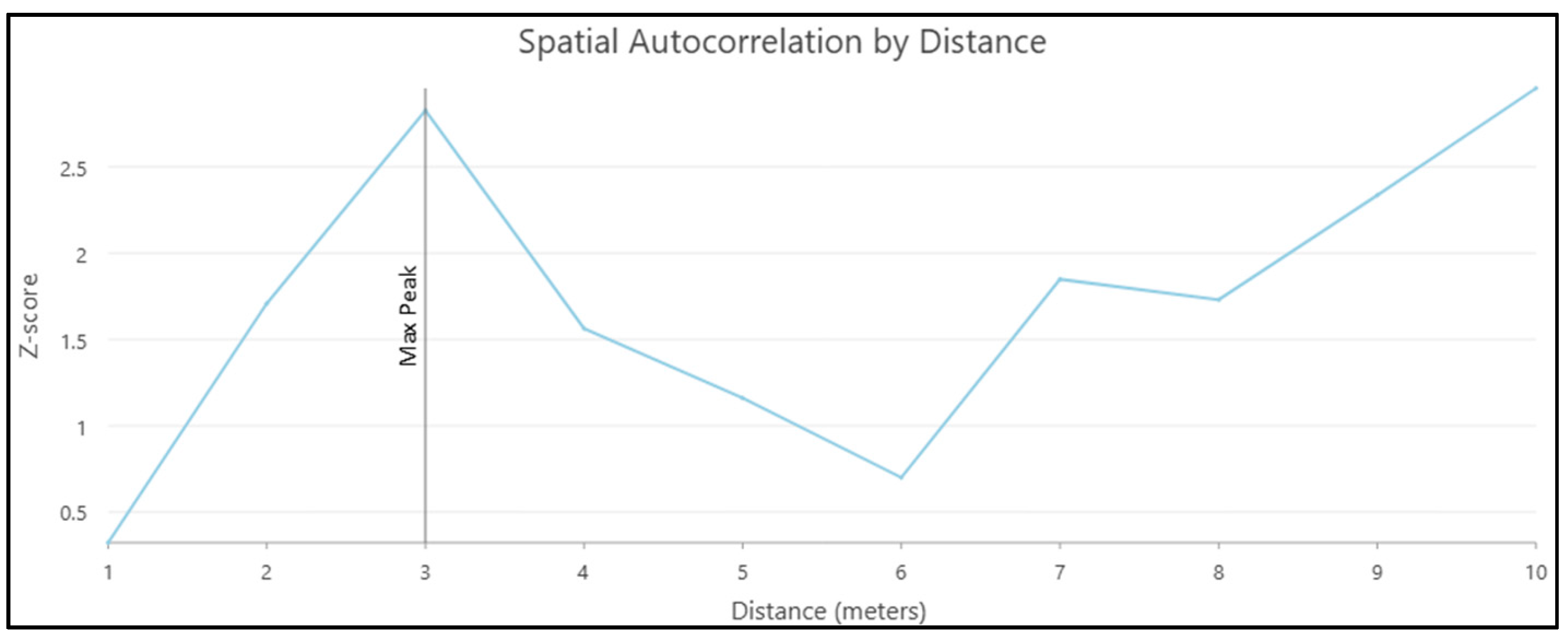
Figure 4.
Comparison of Conceptualization of Distance methods used to calculate Moran’s I. Grouped by method and colored by distance band with a threshold of statistical significance (shown a solid blue line). Z-Scores of methods surpassing threshold listed.
Figure 4.
Comparison of Conceptualization of Distance methods used to calculate Moran’s I. Grouped by method and colored by distance band with a threshold of statistical significance (shown a solid blue line). Z-Scores of methods surpassing threshold listed.
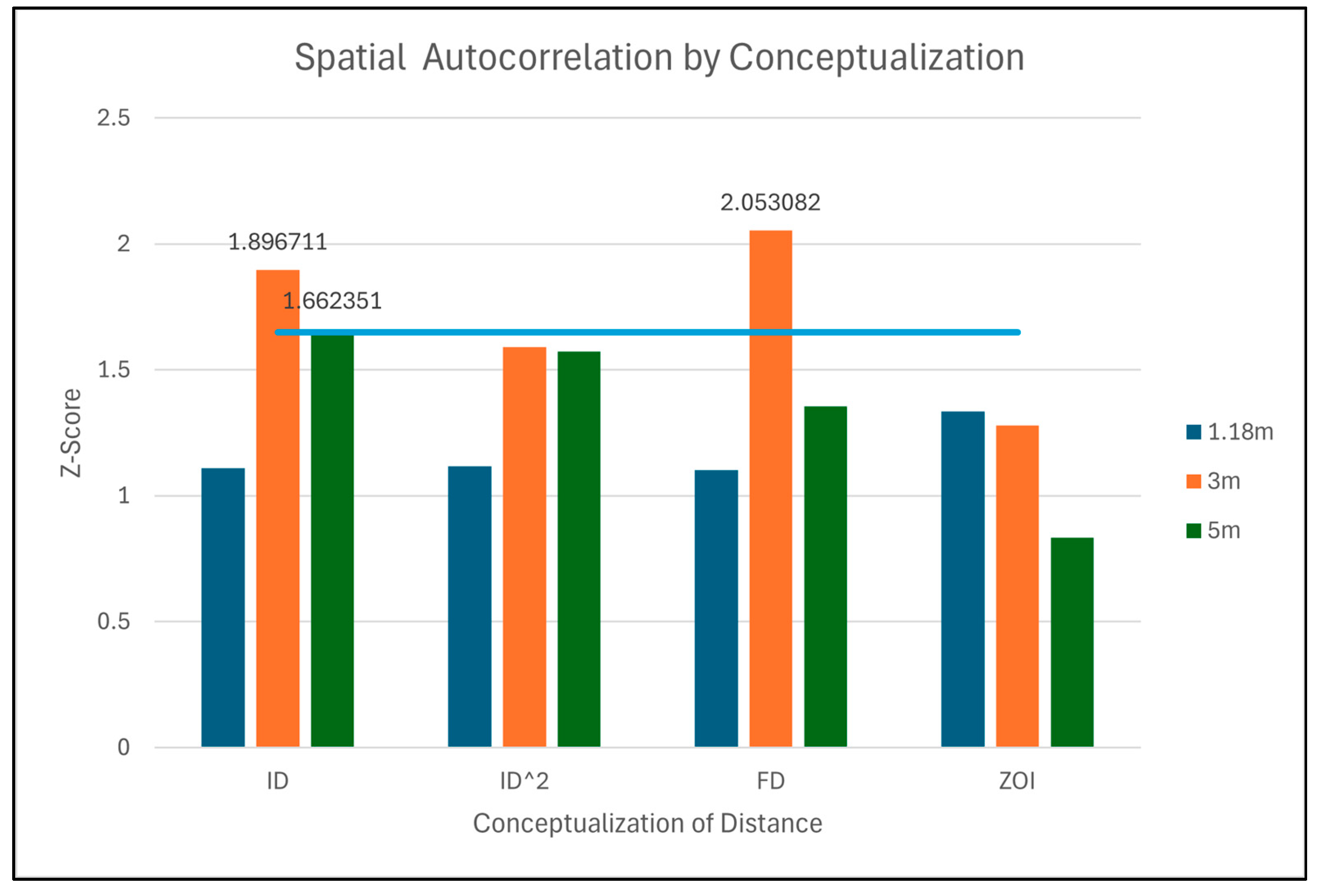
Figure 5.
(a) Well 1 located on bare ground; (b) Well 2 surrounded by trees.
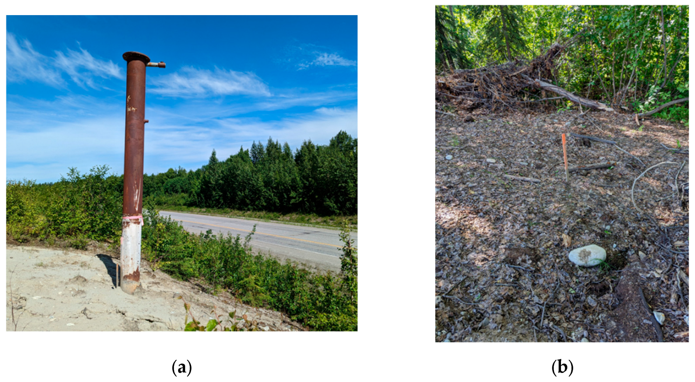

Table 1.
Results from Skewness and Global Moran’s I of Flight tests A-D.
| Test | Skewness | Global Moran’s I Z-score |
|---|---|---|
| A | 1.41 | 1.36 |
| B | 14.35 | 3.23 |
| C | 7.46 | 8.67 |
| D | 7.01 | 2.44 |
Table 2.
Summary of the field test flights in the study area.
| Test | AGL Flight Height | Remediation Phase |
|---|---|---|
| E | 25m | Pre-Remediation |
| E-1 | 25m | Pre-Remediation |
| E-2 | 25m | Pre-Remediation |
| F | 20m | Pre-Remediation |
| G | 25m | Pre-Remediation |
| G-1 | 25m | Pre-Remediation |
| G-2 | 25m | Pre-Remediation |
| H | 20m | Pre-Remediation |
| I | 25m | During |
| J | 25m | During |
Disclaimer/Publisher’s Note: The statements, opinions and data contained in all publications are solely those of the individual author(s) and contributor(s) and not of MDPI and/or the editor(s). MDPI and/or the editor(s) disclaim responsibility for any injury to people or property resulting from any ideas, methods, instructions or products referred to in the content. |
© 2026 by the authors. Licensee MDPI, Basel, Switzerland. This article is an open access article distributed under the terms and conditions of the Creative Commons Attribution (CC BY) license (http://creativecommons.org/licenses/by/4.0/).
Copyright: This open access article is published under a Creative Commons CC BY 4.0 license, which permit the free download, distribution, and reuse, provided that the author and preprint are cited in any reuse.


