
Submitted:
04 February 2026
Posted:
05 February 2026
You are already at the latest version
Abstract
In this note, we show that the methodology used by the DESI collaboration and others for extracting cosmological parameters from 2-point galaxy correlations is fundamentally flawed. The problem with that method is that it is based on the use of a fiducial cosmology to determine the comoving coordinates of galaxies, which are then used to fix parameters, but the mdthod is circular, and is guaranteed to return the fiducial parameters as the optimal solution no matter what model or set of parameters is used. We also point out several arguments against the existence of baryonic acoustic oscillations on large scales, and a significant problem with the FRW model when the latter is used to investigate events at the time of recombination
Keywords:
cosmology
; galaxy correlations
; hubble constant
; dark energy
; cosmological constant
1. Introduction
One of the long-standing problems of cosmology is the disparity between the values of the Hubble constant determined by the standard candle-distance ladder approach and the baryonic acoustic oscillation (BAO) approach [1,2,3,4]. The BAO authors claim that their results support the standard model of cosmology, but the distance ladder authors claim the same thing, and both can’t be right since the respective values of the Hubble constant differ by a considerable amount. In this paper, we are concerned with the BAO 2-point galaxy correlation approach which builds on the fact that there is a peak in the correlation distribution at a distance of [2,5]. The current interpretation of this peak is that it is a result of density concentrations induced by BAO in the matter content of the universe at the time of recombination [5,6]. What we will show is that, first, there are significant problems with the whole idea of BAO on the scale needed to explain the correlation peak, and second, while the peak is real enough, the method used to extract cosmological parameters from it is fundamentally flawed with no way that it can be fixed. We will also point out a different problem with the FRW model that appears when trying to analyze events at the time of recombination.
Before getting to those topics, we will first discuss dark energy. A primary goal of the DESI program (the DE in DESI stands for dark energy) is to determine the origin of dark energy and the value of the cosmological constant. In the next section, we will show that our new model of cosmology provides a full explanation of both, including a formula for the cosmological constant whose value matches the currently accepted Planck value exactly. Following that somewhat off-topic excursion, in the remaining sections, we will point out a number of problems with the BAO model, and with the standard 2-point correlation analysis methodology. Because of these problems, the 2-point correlation determinations of cosmological parameters, including the Hubble constant, are meaningless.
2. Dark Energy and the Cosmological Constant
The idea of a cosmological constant has been around for a long time, but the lack of knowledge about its origin and value didn’t acquire any urgency until the discovery of the accelerated expansion of the universe [7]. At that point, within the context of the FRW model of cosmology, a cosmological constant became necessary to account for the expansion. One of the failings of the FRW model of cosmology is that it does not predict its existence or its value, so it had to be introduced as an ad hoc addition. That is where things stood for about 20 years, but recent DESI results [2,5] hint that the cosmological constant aka dark energy varies with time which creates a really big problem for FRW because the FRW solution of Einstein’s equations is only valid for a cosntant cosmological constant. If the cosmological “constant” varies with time, the FRW model is not longer a solution of Einstein’s equations.
Since the cosmological constant is considered to be a vacuum phenomenon, the logical extension is to think of dark energy as another name for time-varying vacuum energy. With that interpretation, the cosmological constant drops to a secondary role as the value or limit of dark energy at some particular point in time.
With time-varying dark energy, the FRW model fails completely. Our new model of cosmology, on the other hand, gives equations for time-varying dark energy, and predicts a value of the cosmological constant that matches exactly the currently accepted value.
Our new model of cosmology is based on the ideas that the curvature of spacetime must vary with time, and that the self-interaction of vacuum energy requires that the vacuum energy and pressure must be included in the energy-momentum (EM) tensor on the RHS of Einstein’s equations. We have found the exact solution of the resulting equations, and among the results are formulas for the time-varying vacuum energy and pressure [8,9]. Both have non-zero values at infinite time, but their sum, which is the total energy, does vanish at infinite time, and its present-day value is within a factor of 3 of the accepted current value of dark energy. The formula for the scaling is (the parameters are explained in the references)
and clearly, the model predicts the accelerated expansion. The parameter values are , and with , . These are the only two parameters of our model.
Our original EM tensor does not contain a cosmological constant, but in a recent note [10], we show that when the solution energy and pressure are re-expressed in terms of variables which vanish at infinite time, the EM tensor does acquire a cosmological constant whose value is
which agrees exactly with the Planck value of [11].
The DESI hint about a time variation of dark energy is expressed in terms of a simple ad hoc formula, where is the dark energy equation-of-state (EOS) and are supposed to be constants [2,5]. Although the notion of an EOS does not appear in our new model, it is a simple matter to compute the ratio using our original solution formulas for the energy and pressure. The result is shown in Figure 1.
Our value for the parameter is the value of the EOS at the present day and so is a constant. Our prediction of the other parameter is shown in the figure, and it is clearly not a constant. According to our model, its present-day value is , and because , . Our EOS approaches -1 at infinite time so it never crosses into the so-called phantom region. Neither DESI nor others pin down values for the parameters, so we can’t make a direct comparison, but is thought to be negative with a magnidute somewhat larger than our value. The possible values of range from 0.6 to -1.2 or so, with the latter value favored when is equal to our value. The net result is that the FRW EOS does not agree with our solution, but our result is an exact solution of Einstein’s equations, whereas FRW is not even a solution with .
3. BAO
Baryonic acoustic oscillations (BAO) are another idea that has been around for a long time, and many observable phenomena have been attributed to such waves. In spite of its general acceptance, we will present several arguments that show that the idea is unworkable on the large scales necessary to explain, for example, the origin of cosmic structures, or the temperature anisotropies and polarization of the CMB.
BAO emerge from a perturbation approach to Einstein’s equations in which the perturbations were small adjustments to the homogeneous FRW background field equations. The idea itself is that the coupled photon, electron, and proton fluid that filled the universe before recombination supported sound waves that moved away from perturbation sources. Eventually, at the time of recombination, the sound waves dissipated leaving behind matter density highs and lows that supposedly created the temperature anisotropies and polarization of the CMB as well as seeding the later formation of structures by gravitational accretion.
There are, however, many problems with that idea. The perturbation model imagines a wave emerging from a source at the time of nucleosynthesis, which was later received at some distant region of space at the time of recombination. The first problem is that there would not have been just one source, so each such target point would receive waves from sources distributed over a sphere with a radius determined by the sound speed and the time of recombination. Comparing the surface area of that sphere with the maximum size of a coherent source at the time of nucleosynthesis, , we find a count on the order of . That might be an overestimate, but probably not by much. Our target point would thus have received waves from all directions instead of from a single or very limited number of directions. If we consider another point some distance away, it too would have received waves from all directions but from a different set of uncorrelated sources, so the resulting distribution would be an uncorrelated stocastic process. There is just no way that the waves from all those sources could add up a net wave at any such point, and an even greater impossibility is that all these waves from totally uncorrelated sources could add up to a blueprint for the cosmic web whose 1° length scale of was the size of superclusters at the time of recombination.
The next problem is the assumed existence of the gravitational forces necessary for the formation of sound waves. The idea is that in over-dense regions, gravity will pull the matter together. The resulting increase in the scattering rate would raise the temperature, causing in turn, a pressure which would eventually reverse the infall. The resulting pressure gradient would drive matter away from the high-density regions into the low-density regions, where gravitational attraction would again build up a pressure gradient, but in the opposite direction. The result would be a sound wave.
The problem is that while it might work on small scales, it cannot work on scales large enough to explain cosmic structures or the CMB anisotropies. The reason, as we showed in [12], is that throughout the era from nucleosynthesis to a time well beyond recombination, the universe was expanding so rapidly that gravity was completely ineffective on any scale larger than a few lightyears. On scales the size of galaxies or larger, the particles were moving apart far too rapidly for the pressure forces to exist. The universe might have been filled with small sound wave bubbles, but these would not have become organized on the large scales needed to explain the 1° phenomena.
A third problem is that, in order for BAO to have had any effect during recombination on 1° scales, the BAO length scale would have had to match the size of superclusters at that epoch and that constraint is highly model dependent. Given any model, the time of recombination is found by working backwards from the present, starting with the present-day CMB temperature. The BAO length scale, on the other hand, depends on the time interval between nucleosynthesis and recombination working forward. This makes the BAO model highly dependent on the exact time of recombination in relation to the age of the universe.
For an estimate, we can find the recombination time going forward using . This gives where we are using the fact that a 1° angle corresponds to a dimension on the order of . Next, we can estimate the redshift of recombination using . Setting gives . We now use the FRW formula [13] for the look-back time to a source with redshift z. Making the standard assumptions that , we have
In Figure 2, we show the look-back time for , , and for a range of Hubble constants
The first thing we notice is that for , the look-back time is not even remotely the same as the BAO time of recombination. This means that the structure of the FRW model, with the above parameters, forbids that value of the Hubble constant when dealing with events at the time of recombination.
The next thing to notice is that for , the look-back time is negative, which again indicates a structural failing of the FRW model since the look-back time should not be negative for any reasonable value of the Hubble constant, and that cutoff value is greater than the Planck determination for the constant. The FRW failing might well be associated with the fact that the FRW model curvature, k, is a constant. In our new model, which has no such failings, the curvature varies with time. Instead of having a constant value of , its present-day value is , and at the time of recombination, its value was .
After rearranging Equation (3), we solve for the Hubble constant for a range of look-back times and for three values of “”. In Figure 3, we show the results.
The FRW model prediction is that the Hubble constant is essentially a constant, independent of either the look-back time or the redshift. We also see that the predicted value is close to the Planck value, and since the Planck analysis is based on the FRW model, this suggests that the Planck value might be constrained by the structure of the FRW model. For recombination times corresponding to the BAO estimates, the only value that FRW will allow is , and it completely rejects a value of 73.
Another example of a similar failure comes from the FRW field equation for the derivative of the scaling, . With , the differential equation can be solved [13]. The Lemaitre solution can be written
Setting , , we find that which is even further away from the DESI value than 73. On the other hand, to achieve a value of 68, must have the value, so there is a significant inconsistency between the various results.
A fourth issue is with the anisotropy energy budget, which we discuss in [14].
Our new model predicts that with , recombination occurred at which is about an order of magnitude earlier than the FRW BAO estimate. At that time, the BAO length scale would have only been about 5% of the 1° length scale of the cosmic web at recombination, so BAO could not have had anything to do with the origin of the cosmic web even if such waves did exist.
The conclusion is that a BAO origin of cosmic structures and CMB anisotropies on the 1° scale of superclusters, is just not possible.
4. Two-Point Galaxy Density Correlations
The two-point correlation function is a statistical measure found by measuring the distance between all pairs of galaxies, and it has been known for some time that there is a peak in the correlations at a separation of [15]. The BAO idea is that because the sound waves created higher-than-average density regions in the universe which were later responsible for the existence of galaxies, the distribution of galaxies should peak at the BAO sound horizon distance. As we discussed in the previous section, however, there are a number of reasons why the BAO scheme is unworkable.
In our view, the correlation distance of is simply a reflection of the cosmic web with the peak being fixed by the average size of superclusters and large voids. We make that determination based on the fact that, because superclusters are too large for gravity to have had a significant effect on their characteristic dimension, their size at the time of recombination can be found by scaling their present-day size in the same way that the CMB temperature depends only on the scaling. The BAO adherents would say that superclusters are a result of the BAO, but that would require an exact coincidence between the time spans between nucleosynthesis and recombination and between recombination and the present, as discussed in the previous section. According to the scaling predicted by our model, the idea that the correlation peak has anything to do with BAO is a myth. The superclusters still need to be explained, and our new model does present such an explanation [9,16,17].
5. Model Parameter Determination
The main reason for having any interest in the length scale of the correlation peak is the idea that it could be used to constrain parameters of cosmological models. What we will now show is that the idea doesn’t work. To make use of the correlation distance, it is first necessary to determine the comoving coordinates of all galaxies, but the fact is that we have no way of actually measuring coordinate distances in space, so indirect methods must be used. The consequence is that everything known is to a lesser or greater extent, model-dependent. The closest we come to actual distance measurements comes from the distance ladder approach which is based on the idea of standard candles (see references in [14]). That approach is to some extent based on the FRW model, but it does not involve calculations of the look-back time so it avoids the FRW model failure discussed in Section 3. The ladder approach has been implemented in a number of independent ways, which give results that are in good agreement for redshifts out to or a little larger. These are also in excellent agreement with the predictions of our model. For larger values of redshift, the standard candle-based measurements become more difficult with consequent larger error bars. The motivation for the correlation peak method stems from the fact that the required measurements do not become ever more difficult with increasing distance.
The 2-point correlation distance is a comoving coordinate phenomenon. Leaving aside peculiar velocities, all galaxies are at rest in comoving coordinate space, and since their positions don’t change, neither do the actual 2-point correlations. Since on large scales, the universe is generally thought to be homogeneous and isotropic, measurements of the correlations from any observation point at any epoch should return exactly the same result. A corollary to this is that nothing bearing on time or location can be extracted from the correlation length. The idea is to measure the galaxy correlations across the sky and compare the results with the “known” correlation length using simple formulas from the FRW model. The problem is that what is measured are redshifts, but what are needed are comoving coordinates because it is the coordinates that express the correlations. To make the jump, all studies begin by assuming a fiducial model to convert the measured redshifts into comoving radial coordinates, and that is where the whole idea goes wrong. After making the conversions, one then identifies those galaxies that are separated by the correlation length. The final step is to revert to redshift space again using a model, but this time fixing adjustable model parameters along the way. But all one is doing is measuring the parameters of the original fiducial model.
We will go through the process in steps. We start with a large catalogue of galaxies, and for each, we convert from redshift to comoving coordinate using
where represents some fiducial model with parameters . (We are considering galaxies sufficiently distant that we can ignore peculiar velocities other than our own.) The coordinates so determined may or may not match the actual coordinates, but even if they do, we have no way of knowing it.
From this point onward, the usual procedure is to consider the radial and transverse directions separately. According to the FRW model, in the radial direction the coordinate distance between any two galaxies with the same angular coordinates is given by [5,13].
(We note that this formula is specific to the FRW model. It is not true in general.) In terms of our function F, the coordinate difference between galaxies i and j, is
We search the catalogue for pairs of galaxies that form a peak in our “user-created” comoving coordinate space. The actual peak correlation length will generally be different from our “user-created” length, but probably not by very much. Having identified those galaxy pairs, we now revert to redshift space, again using our model, but with adjustable parameters . For each galaxy, the redshift is then given by the inverse formula,
so the redshift difference is given by
Substituting for the original coordinates and , we have
But with , this is an identity. It is true for any fiducial model whatsoever with any set of parameters. The actual correlation length is never part of the process, and it makes no difference whether or not the “user-created” universe matches the actual universe.
The process is circular. With the same model used in both directions, will always be the optimal solution. If, on the other hand, a different model is used for the return trip, the parameters will likely differ, but that is only comparing one model with another, with neither having anything to say about the actual correlation length, or actual cosmological parameters.
Equation (9) returns the ‘measured” redshift difference, and we already know the actual redshift so the equality of the parameters will fix the “measured” Hubble parameter to be that of the fiducial model.
In the transverse direction, the FRW formula (which again is specific to FRW) is
where the galaxies are selected on the basis of having the same redshift [5]. A model error that increases the apparent comoving coordinates of any pair of galaxies will increase the measured correlation length. The actual correlation length angle cannot be measured directly because we don’t know which 2 galaxies are exactly 1 correlation length apart. As before, the fiducial model is used to determine in the “user-created” space. Reverting to the redshift space will again return the original parameters as the optimal solution.
e are back where we started. To be useful as a standard ruler, it wojuld be necessary to determine the actual comoving coordinates without the use of a fudicial model, but we have no way of doing that.
We will now to make two points about the reported results. In Figure 4, we show the calculated comoving coordinates and the scalings for our new model and the FRW model both with over the relevant redshift range. We see that the curves are not far apart. We won’t show it here, but the luminosity distance curves again with are identical for and are not far apart for somewhat larger values of redshift [14].
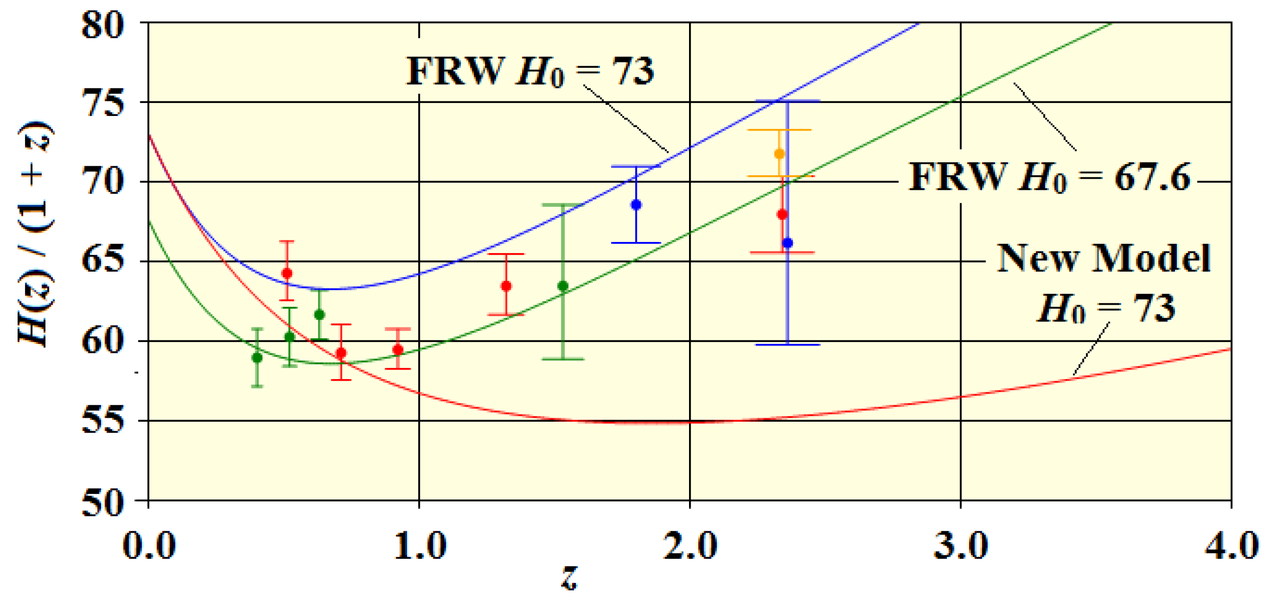
We now show in Figure 5, the familiar plot of the reduced Hubble parameter versus redshift. The data points are from [18,19,20,21,22,23]. We show 3 curves, the FRW model with two values of the Hubble constant, and our new model with .
The point of showing the previous figure is that even though the FRW and new model coordinates and scaling are similar, there is a considerable difference between the FRW and our new model predictions for the reduced Hubble parameter. Thus, one cannot assume that because some properties of two (nonlinear) models are similar, that all properties will be similar.
The main point, however, is that the data points of Figure 5 are all grouped along the FRW curve with . The reason is that all the studies use the same fiducial cosmology with a Hubble constant of 67.6 or a value close to it. As expected, the predicted Hubble constant is the same as the input fiducial constant. If the fiducial Hubble constant were to be changed to 73, the data points will then align with the FRW “73” curve. If our new model was to be used, the data points would group around our new model curve.
6. Conclusions
We have pointed out a number of shortcomings of the BAO model, and have presented a proof that the analysis method used to extract cosmic model parameters from the 2-point galaxy correlation peak is fundamentally flawed. With the elimination of the galaxy correlation determination, (and also the TRGB determination, which is also flawed [14]), only the Planck result remains in tension with . The Planck value is based on their 6-parameter fit to the CMB anisotropy spectrum, but none of those parameters is predicted ahead of time, so the connection with reality is somewhat loose. In addition, we show that the FRW model, which is basic to the Planck analysis method, fails at the look-back times corresponding to recombination, which might have a bearing on the low value of the Planck Hubble constant. We also noted that the FRW solution for the scaling with predicts a Hubble contant that is much larger that 73. On the other hand, to achieve a Hubble constant of 68, a value is needed. This combination indicates an inconsistency in the model.
Funding
No funding was received for this research.
Data Availability Statement
Data sharing not applicable - no new data generated.
Conflicts of Interest
The author declares no conflicts of interest.
Use of Artificial Intelligence
No AI-assisted technologies were used in the development of this article.
Code Availability Statement
This manuscript has no associated code/software.
References
- Perivolaropoulos, L; Skara, F. Challenges for ΛCDM: An update. arXiv 2022, arXiv:2105.05208v3. [Google Scholar] [CrossRef]
- Efstathiou, G. Challenges to the ΛCDM Cosmology. Phil. Trans. R. Soc. A 2025, 383, 20240022. [Google Scholar] [CrossRef] [PubMed]
- Abdalla, E; et al. Cosmology intertwiined: A review of the particle physics, astrophysics, and cosmology associated with the cosmological tensions and anomalies. arXiv 2022, arXiv:2203.06142vf1.
- CERN Courier. The Hubble Tension. 2025. Available online: https://cerncourier.com/a/the-hubble-tension/.
- DESI Collaboration et. al. (2024) DESI 2024 VI: Cosmological Constraints from the Measurements of Baryon Acoustic Oscillations, ArXiv. Available online: https://arxiv.org/abs/2404.03002. [CrossRef]
- Zarrouk, p., et al, The clustering of the SDSS-IV extended Baryon Oscillation Spectroscopic Survey DR14 quasar sample: measurement of the growth rate of structure from the anisotropic correlation function between redshift 0.8 and 2.2. mnras 2018, 477(2), 1639–1663. Available online: https://academic.oup.com/mnras/article/477/2/1639/4907982. [CrossRef]
- Riess, A., et al, Observational Evidence from Supernovae for an Accelerating Universe and a Cosmological Constant, AJ 116 1009. 10.1086/300499. 1998. Available online: https://iopscience.iop.org/article/10.1086/300499.
- Botke, J. C. A Different Cosmology: Thoughts from Outside the Box. Journal of High Energy Physics, Gravitation and Cosmology 2020, 6, 473–566. [Google Scholar] [CrossRef]
- Botke, John C., (2023) Cosmology with Time-Varying Curvature – A Summary, Book chapter, Book, Chapter. Available online: https://www.intechopen.com/online-first/1167416. [CrossRef]
- Botke, J. C. A Note about the Cosmological Constant, Preprint. 2026. Available online: https://www.preprints.org/manuscript/.
- Wikipedia. Cosmological constant. 2025. Available online: https://en.wikipedia.org/wiki/Cosmological_constant.
- Botke, J. C. The Origin of Cosmic Structures Part 1—Stars to Superclusters. Journal of High Energy Physics, Gravitation and Cosmology 2021, 7, 1373–1409. [Google Scholar] [CrossRef]
- M. P. Hobson, et al, (2006) General Relativity, An Introduction for Physicists, Cambridge University Press.
- Botke, J. C. The Origin of Cosmic Structures Part 5—Resolution of the Hubble Tension Problem. Journal of High Energy Physics, Gravitation and Cosmology 2023, 9, 60–82. [Google Scholar] [CrossRef]
- Eisenstein, D.J., et al. (2005) The Astrophysical Journal, 633, 560. Available online: https://iopscience.iop.org/article/10.1086/.
- Botke, J. C. The Origin of Cosmic Structure, Part 4 – Nucleosynthesis. Journal of High Energy Physics, Gravitation and Cosmology 2022, 8(3). Available online: https://www.scirp.org/journal/paperinformation.aspx?paperid=118834. [CrossRef]
- Botke, J. C. Thoughts on the Origin of Our Fractal Universe. Journal of Modern Physics 2025, 16(1). [Google Scholar] [CrossRef]
- DESI Collaboration et al., DESI 2024 III: Baryon Acoustic Oscillations from Galaxies and Quasars. arXiv E-Prints 2024. [CrossRef]
- DESI Collaboration et al., DESI 2024 IV: Baryon Acoustic Oscillations from the Lyman Alpha Forest. arXiv E-Prints 2024. [CrossRef]
- Alam S et al., The clustering of galaxies in the completed SDSS-III Baryon Oscillation Spectroscopic Survey: cosmological analysis of the DR12 galaxy sample. Mon. Not. R. Astron.Soc 2017, 470, 2617–2652. [CrossRef]
- Ata M et al., The clustering of the SDSS-IV extended Baryon Oscillation Spectroscopic Survey DR14 quasar sample: first measurement of baryon acoustic oscillations between redshift 0.8 and 2.2. Mon. Not. R. Astron. Soc. 2018, 473, 4773–4794. [CrossRef]
- Blomqvist M et al., Baryon acoustic oscillations from the cross-correlation of Ly α absorption and quasars in eBOSS DR14. Astron. Astrophys. 2019, 629, A86. [CrossRef]
- de Sainte Agathe V et al., Baryon acoustic oscillations at z = 2.34 from the correlations of Ly α absorption in eBOSS DR14. Astron. Astrophys. 2019, 629, A85. [CrossRef]
Figure 1.
Vacuum EOS.
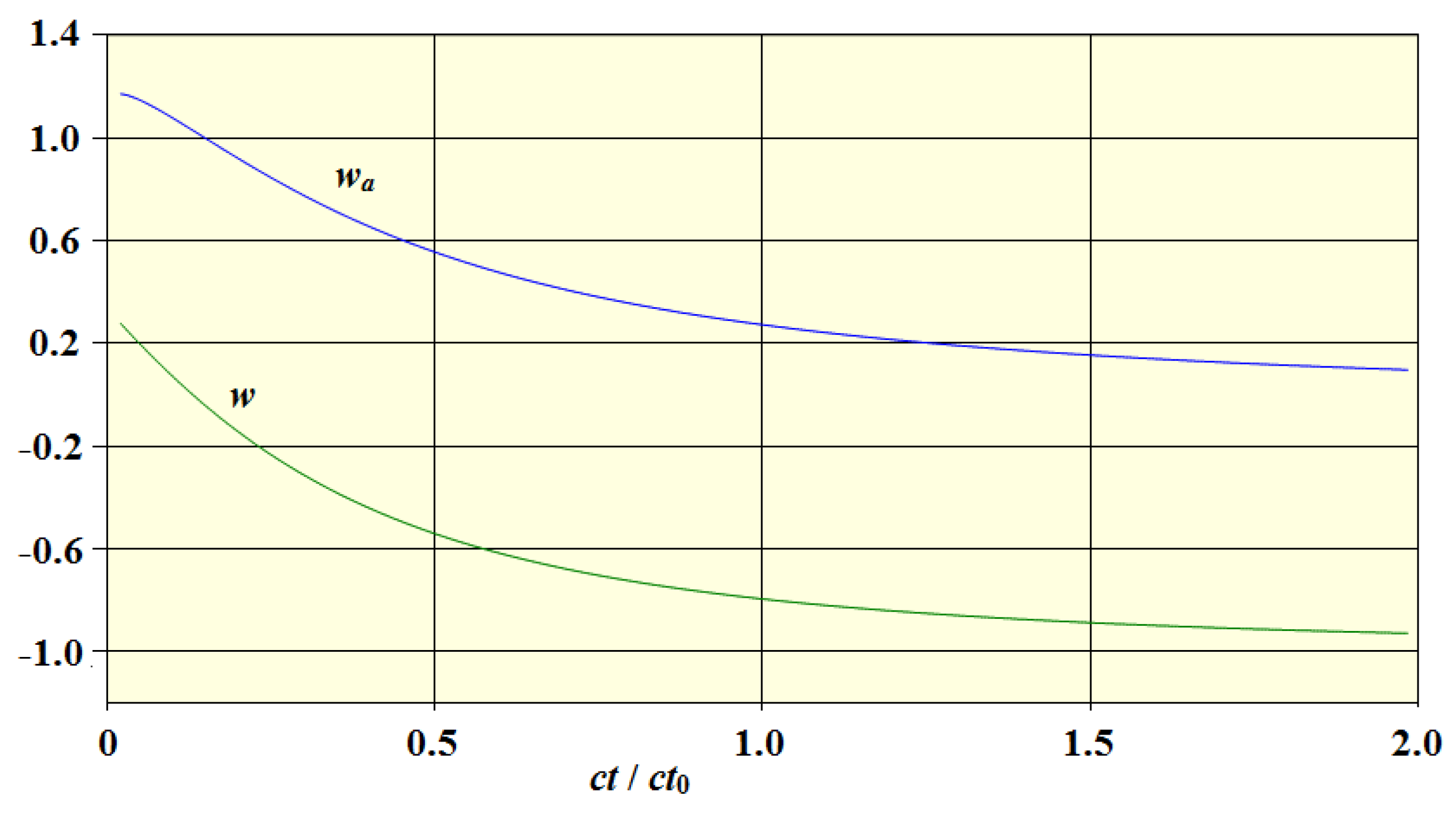
Figure 2.
FRW look-back time versus Hubble constant.
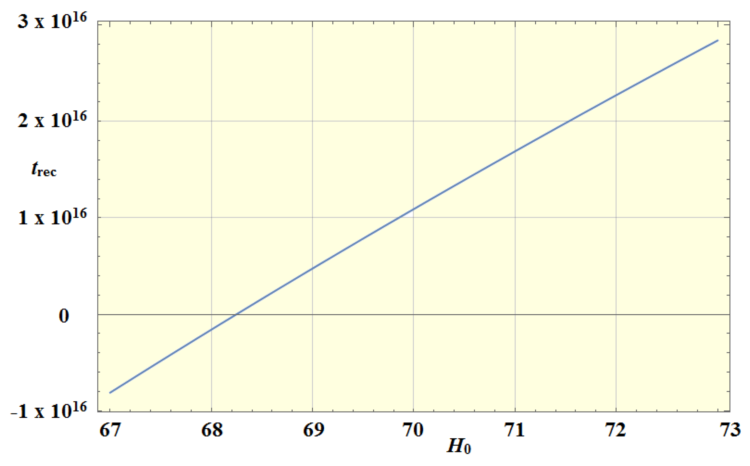
Figure 3.
Hubble constant versus look-back time for 3 values of redshift.
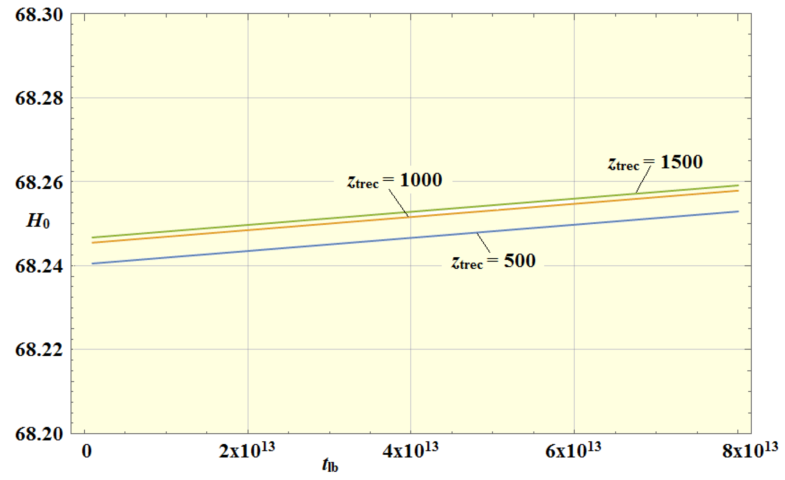
Figure 4.
Comparison of our new model and the FRW model for . The FRW curves are shown in blue.
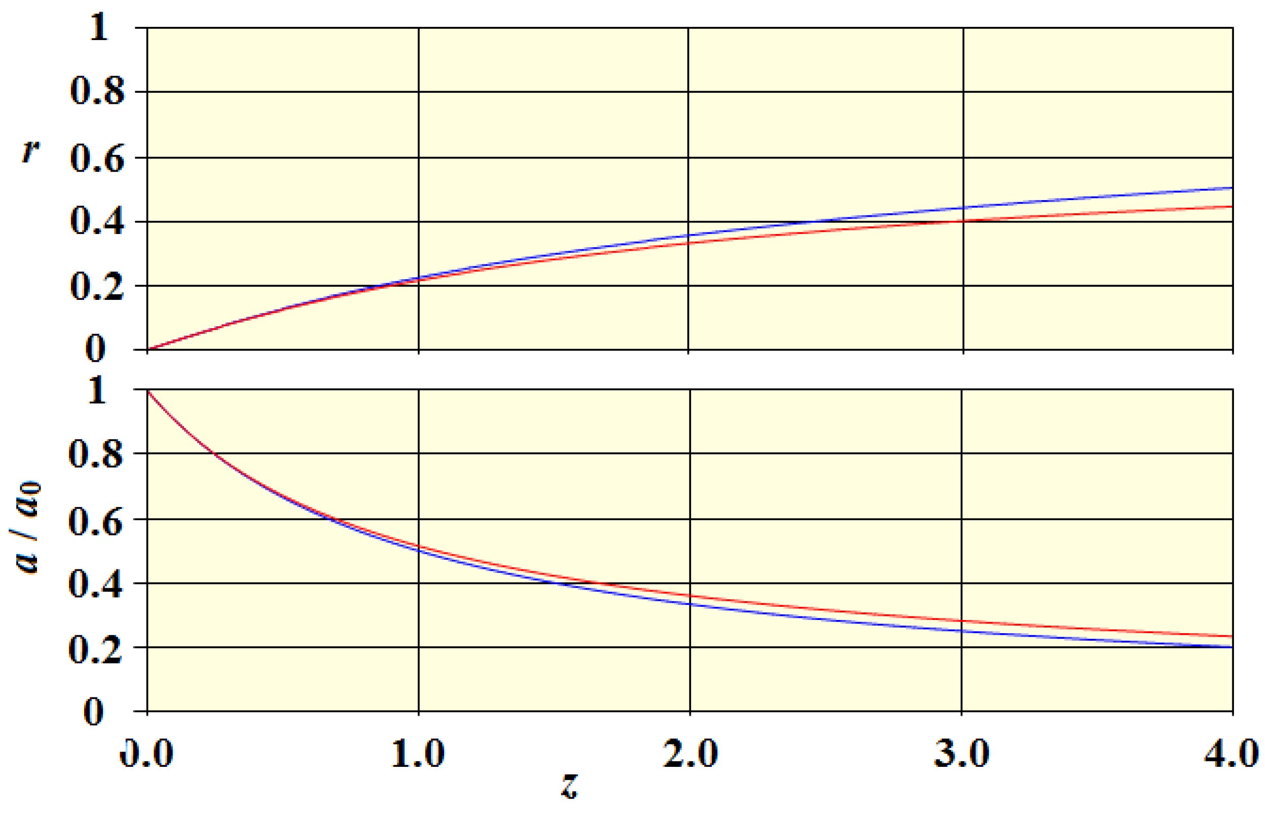
Figure 5.
Reduced Hubble parameter.
Disclaimer/Publisher’s Note: The statements, opinions and data contained in all publications are solely those of the individual author(s) and contributor(s) and not of MDPI and/or the editor(s). MDPI and/or the editor(s) disclaim responsibility for any injury to people or property resulting from any ideas, methods, instructions or products referred to in the content. |
© 2026 by the author. Licensee MDPI, Basel, Switzerland. This article is an open access article distributed under the terms and conditions of the Creative Commons Attribution (CC BY) license.
Copyright: This open access article is published under a Creative Commons CC BY 4.0 license, which permit the free download, distribution, and reuse, provided that the author and preprint are cited in any reuse.


