
Submitted:
04 February 2026
Posted:
06 February 2026
You are already at the latest version
Abstract
Dynamic street-scene reconstruction from sparse viewpoints over long temporal spans is challenged by temporal instability, ghosting near occlusions, and background drift. This paper presents SPT-Gauss, a Gaussian-splatting framework that improves dynamic reconstruction without object-level annotations by combining dense semantic priors with lightweight, parameter-level temporal regularization. SPT-Gauss distills per-pixel semantic features from a frozen 2D foundation model into 4D Gaussian primitives, estimates static and dynamic regions via a dual-evidence motion mask, and regularizes temporal parameters through a semantic-guided velocity constraint and a static-lifetime prior to suppress spurious background motion. Experiments on the Waymo Open Dataset and KITTI show consistent improvements over representative baselines in both 4D reconstruction and novel-view synthesis, with reduced temporal artifacts and improved fidelity in motion-challenging regions.
Keywords:
dynamic scene reconstruction
; 4D Gaussian splatting
; temporal consistency
; semantic distillation
; novel view synthesis
; autonomous driving
1. Introduction
Autonomous driving in open-road environments increasingly benefits from dynamic 3D representations that are measurable, renderable, and editable throughout the perception–prediction–planning pipeline [1]. High-fidelity reconstruction provides geometric priors and occlusion completion for downstream tasks such as detection, segmentation, and tracking, while photorealistic neural rendering enables replay of rare events for adversarial testing and closed-loop evaluation. From a systems perspective, incremental updates and long-term maintenance of 3D/4D assets across edge, roadside, and cloud deployments can reduce operational costs and improve robustness in complex traffic scenarios.
Novel view synthesis (NVS) and neural rendering have progressed from implicit volumetric radiance fields such as NeRF [1] to a variety of acceleration and sparsification techniques, including multi-resolution hash grids, explicit radiance tensors, and factorized plane representations [2,3,4,5]. More recently, explicit point-based formulations have drawn increasing attention due to their efficiency and editability. In particular, 3D Gaussian Splatting (3DGS) enables real-time rendering and fast convergence for static scenes via differentiable rasterization and depth-ordered compositing [6]. Extending 3DGS to dynamic scenes typically requires introducing time-varying parameters (e.g., positions, rotations, opacity, or learned deformations) and enforcing temporal regularization to reduce drift, ghosting, and flickering across frames [7,8,9,10,11,12,13,14,15,16].
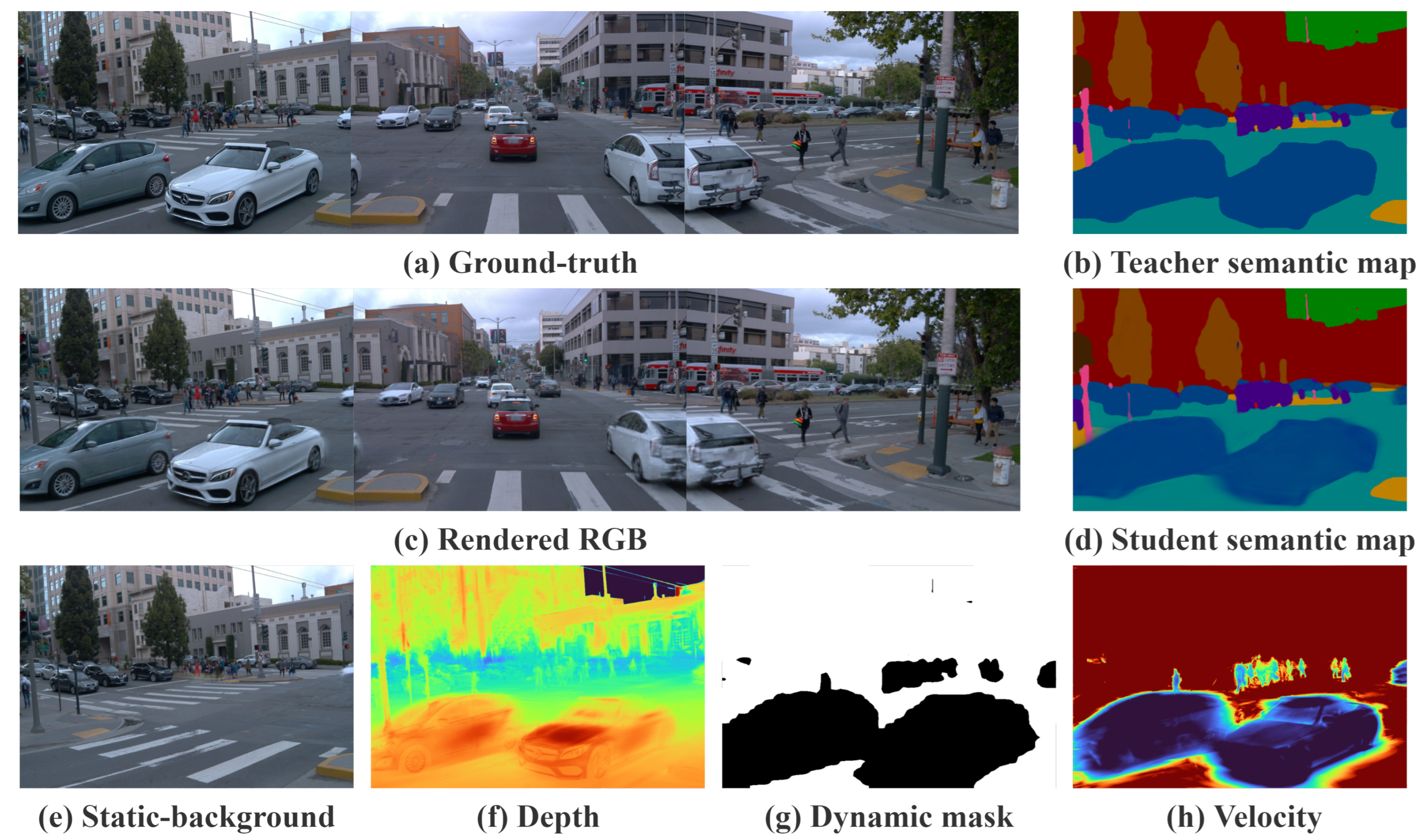
Figure 1.
Overview of SPT-Gauss. (a) Ground-truth view; (b) teacher semantic map; (c) rendered RGB; (d) student semantic map after 2D-to-4D distillation; (e) stabilized static-background rendering enabled by temporal constraints; (f) pseudo-colored depth; (g) motion mask from dual-evidence fusion; (h) per-pixel velocity magnitude.
Among dynamic Gaussian formulations, periodic-vibration models provide a compact way to incorporate time with minimal changes to the explicit representation. They parameterize each primitive with differentiable temporal oscillations and lifetime decay, allowing static background and moving agents to be represented under a unified set of temporal parameters while preserving efficiency and editability [12,17]. Related directions jointly estimate scene motion and appearance using neural flow or spatiotemporal Gaussian coupling, enabling label-efficient dynamic reconstruction and multimodal synthesis (e.g., RGB, depth, and optical flow) [13,18]. Instruction- or constraint-driven editing has also been explored on Gaussian backbones [19].
Dynamic reconstruction in urban driving remains challenging due to large-scale structure, persistent motion, frequent occlusions, and sparse viewpoints. Methods with object-level priors decompose background and agents using 3D boxes, masks, or tracking, offering controllable rendering and editing [20,21,22,23]. However, such pipelines depend on substantial annotations and engineering effort. Weakly supervised and self-supervised approaches reduce reliance on object-level labels via scene decomposition, canonicalization, and deformation modeling, but they often suffer from background drift and temporal instability over long sequences or under heavy occlusions. Recent work mitigates these issues with staged training, temporal consistency losses, and geometry-aware regularization [7,24,25,26,27]. In parallel, feature distillation injects high-level semantics from 2D foundation models into explicit 3D/4D representations, supporting retrieval, editing, and weak-label propagation [28,29]. Large-scale encoders such as CLIP, DINOv2, SAM, LSeg, and Mask2Former provide strong teacher signals for dense semantics [30,31,32,33,34,35].
These observations motivate a practical question: how can one improve temporal stability and dynamic reconstruction quality in driving scenes without relying on object-level annotations, while preserving the efficiency and editability of Gaussian splatting? In this work, we propose SPT-Gauss, a dynamic Gaussian framework that integrates semantic priors with lightweight parameter-level temporal constraints under a periodic-vibration model. The framework consists of three components. First, it performs 2D-to-4D semantic distillation by transferring pixel-aligned features from a frozen 2D foundation model to 4D Gaussians, equipping each primitive with a compact semantic vector. Second, it constructs a dual-evidence motion mask by combining teacher–student feature discrepancy with semantic priors, and stabilizes the separation with temporal voting. Third, it introduces two parameter-level temporal constraints, including a semantic-guided velocity constraint and a static-lifetime prior, which regularize temporal parameters to suppress background drift and reduce long-sequence jitter.
Contributions are summarized as follows: (1) We present a 2D-to-4D semantic-distillation scheme that transfers dense semantics from 2D foundation models to 4D Gaussians, yielding compact per-primitive semantic vectors for analysis and editing. (2) We propose a dual-evidence motion mask that fuses teacher–student feature discrepancy with semantic priors, and apply temporal voting to obtain robust static/dynamic separation for supervision routing and temporal regularization. (3) We introduce parameter-level temporal constraints, including a semantic-guided velocity constraint and a static-lifetime prior, to reduce background drift and temporal jitter and to improve long-sequence stability and rendering quality.
2. Materials and Methods
This section describes the proposed semantic- and temporal-prior driven dynamic Gaussian framework, SPT-Gauss. As shown in Figure 2, the pipeline consists of five parts: preliminaries, 2D-to-4D semantic distillation, dual-evidence motion masking, semantics-driven temporal constraints, and optimization. The framework integrates dense 2D semantic priors with lightweight temporal modeling under a periodic-vibration Gaussian representation, and it is trained without object-level annotations.
2.1. Preliminaries: 3DGS and PVG
3D Gaussian Splatting (3DGS) represents a scene using a set of anisotropic Gaussian primitives. Each primitive stores a 3D center, anisotropic scale and rotation, opacity, and appearance parameters. Rendering is performed by differentiable rasterization and depth-ordered alpha compositing [6,36]. A single 3D Gaussian is defined as
where is the 3D center and is the covariance parameterized by rotation and scale . After projection to the image plane, the 2D covariance is approximated by
where is the world-to-camera extrinsic transform and is the Jacobian approximation of perspective projection. For a pixel, the rendered color is computed by depth-sorted -compositing:
where depends on the primitive opacity and its projected footprint at the pixel, and denotes the appearance.
Standard 3DGS is time-invariant, which limits its applicability to road scenes with persistent motion (e.g., vehicles and pedestrians). Periodic Vibration Gaussians (PVG) introduce a compact temporal parameterization, in which each primitive follows a differentiable oscillatory trajectory and a lifetime-controlled visibility decay around a peak time [17]. For each primitive, PVG defines a temporal period l, a velocity vector , and a lifetime scale :
The primitive state at time t is , and the rendered image is
with intrinsics and extrinsics . We define the staticness ratio as
where larger indicates longer visibility relative to the oscillation period. When and , PVG reduces to standard 3DGS. In this way, static and dynamic content share the same rendering backbone and are differentiated only by temporal parameters .
2.2. 2D-to-4D Semantic Distillation (SD)
Reconstruction losses alone may not reliably disentangle camera-induced appearance changes from real-world motion. We therefore distill dense semantic features from a frozen 2D foundation model into the 4D Gaussian representation, so that each primitive carries a compact semantic vector used for prior injection and motion masking.
We adopt Language-driven Segmentation (LSeg) as the teacher [33], whose pixel features are aligned to the CLIP text space [30]. Given an RGB frame at time t, the teacher feature map is
On the student side, each primitive is assigned a learnable semantic vector . Analogous to RGB rendering, the student semantic feature at pixel is computed by alpha-composited aggregation over the depth-sorted visible set :
where are the standard compositing weights induced by -blending (i.e., ). To match the teacher feature dimensionality, we apply a lightweight linear projection head :
We minimize a pixel-wise distillation loss:
where is the pixel set at the current resolution. After optimization, semantics are embedded into per-primitive vectors and propagated over time through PVG.
2.3. Dual-Evidence Motion Mask (DEMM)
Using the teacher features and the rendered student semantics , we estimate a motion mask from two complementary cues: (i) teacher–student feature discrepancy and (ii) a semantic prior indicating regions that are likely static. The fusion yields a soft static probability map , which is used as a differentiable weight in temporal constraints; binary masks can be obtained for visualization or evaluation.
2.3.1. Teacher–student feature discrepancy
For static surfaces, multi-frame observations correspond to the same world points and the student features are expected to match the teacher features. Pixels on moving objects or near occlusion boundaries tend to show discrepancies. We define a pixel-wise cosine dissimilarity:
Larger indicates a higher likelihood of motion or inconsistent alignment.
2.3.2. Semantic prior and fusion
Using the teacher model, we obtain class scores and form a soft static prior by summing scores over a set of static-leaning categories (e.g., road, building, sky):
We fuse the two cues with a logistic regressor to produce the static probability:
where is the sigmoid and are learnable scalars. For binary masks, we threshold :
with by default.
Temporal voting (conservative merge).
To reduce frame-wise errors, we perform temporal voting over a window centered at t (e.g., ). We adopt a conservative merge strategy: a pixel is marked static only if it is consistently static across the window (intersection), while it is marked dynamic if it is predicted dynamic in any frame (union):
In training, we use the soft weight (not binarized) for differentiability; the temporally voted binary masks are used for qualitative visualization and optional evaluation.
2.4. Semantics-Driven Temporal Constraints
We impose temporal constraints to suppress spurious motion on static regions while maintaining temporal coherence for dynamic targets. The constraints are applied at the parameter level of PVG by using (i) the pixel-level static probability and (ii) a back-projected per-primitive static weight , which measures how strongly primitive i contributes to pixels with high static probability.
2.4.0.2. Back-projected static weight.
For a frame at time t, we define
where are compositing weights, is the pixel domain, and is a small constant. When summing losses across a mini-batch, we use averaged over frames in the batch.
2.4.1. Semantic Velocity Constraint (SVC)
We apply a semantic gate to modulate the PVG velocity magnitude. For primitive i, we compute a gate from its semantic vector:
where and are learnable parameters. The PVG trajectory uses (all other rendering components remain unchanged). To measure projected motion, we compute a symmetric-step displacement in the image plane using a fixed :
where denotes camera projection. We penalize projected motion on pixels with high static probability:
2.4.2. Static-Lifetime Prior (SLP)
Constraining instantaneous speed may still allow slow drift over long sequences. We therefore regularize the PVG staticness ratio for primitives that contribute to static regions. For each primitive, define
and impose a lower bound weighted by the back-projected static weight:
where controls the preference for long lifetime relative to the oscillation period.
2.5. Optimization
We optimize the Gaussian parameters using a reconstruction loss combined with semantic distillation and temporal constraints. The photometric term is a weighted sum of pixel-wise and SSIM:
In addition, LiDAR point clouds are projected onto the camera plane to form sparse inverse-depth maps [37,38]. Let denote the sparse inverse depth and the validity mask. We use a masked depth loss:
where is the rendered inverse depth.
We regularize semantic vectors and PVG velocities with
The overall objective is
To avoid over-penalizing motion before geometry and appearance stabilize, we apply a warm-start schedule: (constant); increases linearly from 0 to over the first iterations; ; and the staticness lower bound increases linearly from to over the first iterations. Unless otherwise specified, we use for and (implemented by scaling the corresponding terms), and set in depending on scene sparsity.
3. Results
3.1. Experimental Setup
3.1.1. Datasets
We evaluate SPT-Gauss on two widely used large-scale road-scene benchmarks, the Waymo Open Dataset and KITTI [37,38]. Waymo Open provides synchronized multi-camera and multi-LiDAR sequences with accurate timestamps and calibration. Following PVG [17], we select four challenging urban sequences. Three forward-facing cameras are used for training at , and a fourth camera is held out for novel-view synthesis (NVS) evaluation. KITTI provides multi-view camera streams and vehicle poses. Following the SUDS protocol [39], we select motion-rich sequences and use the left–right stereo pair () for training and evaluation.
3.1.2. Evaluation Protocols
We use two evaluation protocols on Waymo for clarity and reproducibility. (i) Main comparison protocol: all methods in Table 1 and Table 2 are evaluated on the same set of four sequences following PVG [17], with identical camera splits for reconstruction and NVS. (ii) Ablation protocol: the ablation study in Table 3 is conducted on a reduced subset of Waymo sequences to enable faster and controlled analysis of module behaviors. Therefore, absolute values in Table 3 are intended for relative comparison among ablated variants only and are not directly comparable to the main comparison results.
3.1.3. Metrics
We report PSNR (↑), SSIM (↑), and LPIPS (↓) [40,41] for 4D reconstruction and NVS. To analyze reconstruction quality across different regions, we additionally report static-region PSNR (S-PSNR) and dynamic-region PSNR (D-PSNR) computed using estimated motion masks. These region-wise metrics provide complementary insights into static/dynamic behavior; they are used consistently across methods under the same protocol. We compare against representative NeRF-based and Gaussian-splatting-based baselines, including 3DGS [6], SUDS [39], StreetSurf [42], EmerNeRF [27], MARS [43], PVG [17], and CoDa-4DGS [26].
3.1.4. Implementation Details
All experiments are performed on one NVIDIA vGPU with 48 GB memory. Gaussians are initialized from the ego-LiDAR point cloud (instead of SfM). Time-related parameters are initialized neutrally (, , ). For stable early optimization, the linear layers used for semantic gating and evidence fusion are initialized to produce near-neutral outputs (so that and at initialization). The LSeg teacher is frozen; its per-pixel features are cached offline (optionally quantized to 8-bit) to reduce memory usage during training. We use Adam (, ) with an initial learning rate of , cosine-decayed to [44,45]. The batch size is 2, gradients are clipped at , and we adopt a two-stage resolution curriculum: a pre-warm phase at one-quarter resolution followed by a ramp to full resolution to jointly optimize distillation and temporal constraints. Loss weights follow the warm-start schedule in Equation (25).
3.2. Quantitative Evaluation
Table 1 summarizes the main results on Waymo Open and KITTI under the main comparison protocol. Across both benchmarks, SPT-Gauss improves PSNR/SSIM and reduces LPIPS compared with recent Gaussian-based baselines such as PVG and CoDa-4DGS. Table 2 reports performance on dynamic regions of Waymo. SPT-Gauss improves D-PSNR by dB and D-SSIM by over PVG under the same evaluation protocol, suggesting that incorporating semantic priors and parameter-level temporal constraints can improve reconstruction quality in motion-dominant areas.
3.3. Qualitative Evaluation
Figure 3 presents qualitative comparisons on Waymo Open and KITTI. Gaussian-based dynamic representations such as PVG and CoDa-4DGS can exhibit temporal artifacts in challenging regions, including ghosting near occlusion boundaries and background drift around moving objects. SPT-Gauss reduces these artifacts in many cases and produces visually more stable renderings, especially in static structures while retaining motion details.
Figure 4 further compares dynamic–static decomposition between PVG and SPT-Gauss. PVG may show motion leakage into the static layer and aliasing artifacts in the dynamic layer. In contrast, SPT-Gauss yields cleaner separation in the shown examples, with dynamic components concentrating on moving objects and static components maintaining sharper textures.
4. Discussion
4.1. Ablation Study and Mechanism Analysis
We conduct an ablation study on Waymo under the ablation protocol (reduced subset) to analyze the contribution of each component. All training configurations are kept identical across variants, except for disabling the corresponding module. Because the submodules in SPT-Gauss are coupled (e.g., motion masking and temporal constraints rely on distilled semantics), removing an upstream component can change the behavior of downstream modules. Therefore, the ablation results are primarily used to compare variants within the same protocol and to interpret module interactions.
Table 3 summarizes the ablation results on the reduced subset. Disabling any component degrades performance, indicating complementary contributions of semantic distillation, motion masking, and parameter-level constraints. Removing SD reduces reconstruction metrics, consistent with the role of dense semantic guidance. Removing DEMM or SVC mainly affects dynamic-region performance, suggesting that reliable motion separation and velocity regularization are important for motion-dominant areas. Removing SLP tends to reduce long-term stability, consistent with its role in discouraging slow drift.
To illustrate the role of semantic distillation in motion estimation, Figure 5 compares motion masks with and without SD. Without semantic guidance, masks can be noisier and may activate on background regions, while enabling SD typically yields more compact dynamic regions and cleaner static areas in the shown examples.
4.2. Limitations and Future Work
SPT-Gauss relies on the quality and domain coverage of the teacher semantic model, and performance can degrade under conditions that are under-represented by the teacher or training data (e.g., extreme lighting changes, adverse weather, or sensor noise). In addition, periodic temporal parameterization may be less expressive for non-periodic, abrupt motions. Future work will explore domain-robust semantic distillation, more expressive temporal parameterizations, and stronger cross-sensor constraints to improve robustness in diverse driving conditions.
5. Conclusions
This paper presents SPT-Gauss, a dynamic Gaussian framework that integrates dense 2D semantic priors with parameter-level temporal constraints under a periodic-vibration representation, without requiring object-level annotations. The method distills per-primitive semantic vectors from a frozen 2D foundation model and uses a dual-evidence motion mask to support static/dynamic separation. By regularizing temporal parameters via a semantic-guided velocity constraint and a static-lifetime prior, SPT-Gauss reduces background drift and improves temporal stability in long driving sequences while preserving the efficiency and editability of Gaussian splatting. Experiments on Waymo Open and KITTI demonstrate consistent improvements over representative baselines in both reconstruction and novel-view synthesis, with additional gains in motion-dominant regions under the same evaluation protocol.
6. Patents
There are no patents resulting from this work.
Supplementary Materials
The following supporting information can be downloaded at the website of this paper posted on Preprints.org.
Author Contributions
Conceptualization, Q.D. and S.G.; methodology, Q.D.; software, Q.D. and K.R.; validation, M.H., J.L. and S.L.; formal analysis, Q.D.; investigation, K.R.; resources, S.G.; data curation, K.R.; writing—original draft preparation, Q.D.; writing—review and editing, S.G.; visualization, Q.D.; supervision, S.G.; project administration, S.G.; funding acquisition, S.G. All authors have read and agreed to the published version of the manuscript.
Funding
This research received no external funding.
Institutional Review Board Statement
Not applicable.
Informed Consent Statement
Not applicable.
Data Availability Statement
The publicly available dataset Waymo Open Dataset was analyzed in this study and can be found here: https://waymo.com/open/, accessed on 31 January 2026. The publicly available dataset KITTI Vision Benchmark Suite was analyzed in this study and can be found here: https://www.cvlibs.net/datasets/kitti/, accessed on 31 January 2026.
Acknowledgments
We thank the anonymous reviewers for their constructive comments.
Conflicts of Interest
The authors declare no conflicts of interest.
Abbreviations
The following abbreviations are used in this manuscript:
| 3DGS | 3D Gaussian Splatting |
| PVG | Periodic Vibration Gaussian |
| NVS | Novel View Synthesis |
| LiDAR | Light Detection and Ranging |
| SPT-Gauss | Semantics-driven Periodic Temporal Gaussian |
| SD | Semantic Distillation |
| DEMM | Dual-Evidence Motion Mask |
| SVC | Semantic Velocity Constraint |
| SLP | Static-Lifetime Prior |
| SSIM | Structural Similarity Index Measure |
| LPIPS | Learned Perceptual Image Patch Similarity |
References
- Mildenhall, B.; Srinivasan, P.P.; Tancik, M.; Barron, J.T.; Ramamoorthi, R.; Ng, R. NeRF: Representing Scenes as Neural Radiance Fields for View Synthesis. In Proceedings of the ECCV, 2020. [Google Scholar]
- Müller, T.; Evans, A.; Schied, C.; Keller, A. Instant Neural Graphics Primitives with a Multiresolution Hash Encoding. ACM Transactions on Graphics (SIGGRAPH), 2022. [Google Scholar]
- Yu, A.; Li, R.; Tancik, M.; Li, H.; Ng, R.; Kanazawa, A. Plenoxels: Radiance Fields without Neural Networks. In Proceedings of the CVPR, 2022. [Google Scholar]
- Chen, A.; Xu, Z.; Geiger, A.; Yu, J.; Su, H. TensoRF: Tensorial Radiance Fields. In Proceedings of the ECCV, 2022. [Google Scholar]
- Lindell, D.B.; Martel, J.N.P.; Chan, E.R.; Wetzstein, G.; Barron, J.T.; Mildenhall, B.; Tancik, M.; Sitzmann, V.; Yu, A.; Fridovich-Keil, B. K-Planes: Explicit Radiance Fields in Space, Time, and Appearance. In Proceedings of the Proc. IEEE/CVF Conf. on Computer Vision and Pattern Recognition (CVPR), 2023. [Google Scholar]
- Kerbl, T.; Kopanas, G.; Leimkühler, T.; Drettakis, G. 3D Gaussian Splatting for Real-Time Radiance Field Rendering. arXiv 2023. arXiv:2308.04079. [CrossRef]
- Luiten, J.; Kopanas, G.; Trulls, E.; Geiger, A. Dynamic 3D Gaussians: Tracking by Persistent Dynamic Gaussians over Time. arXiv 2023, arXiv:2308.09713. [Google Scholar]
- Yang, Z.; Nan, L.; Vallet, B.; Pollefeys, M.; Chen, L. Deformable 3D Gaussians for High-Fidelity Monocular Dynamic Scene Reconstruction. In Proceedings of the Proc. IEEE/CVF Conf. on Computer Vision and Pattern Recognition (CVPR), 2024. [Google Scholar]
- Bae, J.; Park, S.; Choi, J.; Cho, M.; Hong, S.; Park, K. Per-Gaussian Embedding-Based Deformation for Deformable 3D Gaussian Splatting. arXiv 2024. arXiv:2404.03613.
- Wan, D.; Li, X.; Yang, Y.; Ji, Y.; Yao, Y.; Quan, L. Superpoint Gaussian Splatting for Real-Time High-Fidelity Dynamic Scene Reconstruction. In Proceedings of the Proc. Int. Conf. on Machine Learning (ICML) Workshops / PMLR, 2024. [Google Scholar]
- Chen, Z.; Liu, B.; Liu, Z.; Lin, D.; Dai, B. MotionGS: Explicit Motion Guidance for Deformable 3D Gaussian Splatting. arXiv 2024. arXiv:2403.12279.
- Wu, W.; Hu, K.; Zhao, F.; Ding, Y.; Wang, Z.; Chen, J.; Su, H. 4D Gaussian Splatting for Real-Time Dynamic Scene Rendering. In Proceedings of the Proc. IEEE/CVF Conf. on Computer Vision and Pattern Recognition (CVPR), 2024. [Google Scholar]
- Lin, Y.C.; et al. Gaussian-Flow: 4D Reconstruction with Dynamic 3D Gaussian Particles. In Proceedings of the Proc. IEEE/CVF Conf. on Computer Vision and Pattern Recognition (CVPR), 2024. [Google Scholar]
- Huang, Y.; Zhou, K.; Sun, B.; Lin, L.; Wong, X.; Shen, L. 4D-Rotor Gaussian Splatting for Real-Time Rendering of Dynamic Scenes. arXiv 2024. arXiv:2411.10970.
- Li, W.; Zhang, Z.; Dong, X.; Wu, J.; Qin, J.; Wang, K.; Li, H.; Zhu, S.; Dai, J.; Wang, W.; et al. S3-GS: Semi-supervised Structure-aware Gaussian Splatting with Limited Labeled Data. arXiv 2024. arXiv:2411.00184.
- Yang, F.; Ma, F.; Guo, Y.C.; Ren, S.; Zhong, Y.; Zhang, G.; Qi, X.; Jia, J. 3DGS2: Robust Wide-Baseline Gaussian Splatting via Multi-View Consistent Editing. arXiv 2024. arXiv:2403.16697.
- Chen, Y.; Gu, C.; Jiang, J.; Zhu, X.; Zhang, L. Periodic Vibration Gaussian: Dynamic Urban Scene Reconstruction and Real-Time Rendering. arXiv 2023. arXiv:2311.18561. [CrossRef]
- Mo, S.; Wu, H.; Cai, R.; Zhu, J.; Mao, J.; Wang, Y.; Luo, H.; Li, H.; Wang, X.; Adler, D.; et al. SplatFlow: Predicting Dense 2D Tracks for Deformable 3D Gaussian Splatting. arXiv 2024. arXiv:2404.10663.
- Zhang, H.; Pan, Z.; Liu, Y.; Wei, X.; Shi, D.; Zhao, S.; Su, H. Instruct-4DGS: Efficient Dynamic Scene Editing via 4D Gaussian Splatting. arXiv arXiv:2411.18618.
- Li, D.; Wang, X.; Sun, J.; Dai, Y.; Bai, H.; Sun, M.; Luo, P.; You, Y.; Qiao, Y.; Shao, J. DrivingGaussian: Composite Dynamic 3D Scene Representation for Autonomous Driving. In Proceedings of the Proc. IEEE/CVF Conf. on Computer Vision and Pattern Recognition (CVPR), 2024. [Google Scholar]
- Yan, Y.; Lin, H.; Zhou, C.; Wang, W.; Sun, H.; Zhan, K.; Lang, X.; Zhou, X.; Peng, S. Street Gaussians for Modeling Dynamic Urban Scenes. In Proceedings of the European Conference on Computer Vision (ECCV), 2024. [Google Scholar]
- Wong, Z.; Jiang, Y.; Luo, X.; Qi, G.J.; Song, L.; Zhang, W. OmniRe: Unified Omnidirectional Scene Representation. arXiv 2024. arXiv:2411.17384.
- Faigl, J.; Zhang, K.; Barath, D.; Sattler, T.; Pollefeys, M. DrivingGaussian++: Unified Factorized Dynamic Gaussians for City-Scale Street View Synthesis with 3D Detection Refinement. arXiv 2024. arXiv:2409.18884.
- Lee, I.; Yoo, J.; Jo, S.; Baek, S.; Hong, S.; Cho, M. Guess The Unseen: Dynamic 3D Scene Reconstruction from Partial 2D Glimpses. In Proceedings of the Proc. IEEE/CVF Conf. on Computer Vision and Pattern Recognition (CVPR), 2024. [Google Scholar]
- Jia, Z.; Pan, Z.; Wang, R.; Xia, S.; Li, M.; Chen, B.; Dai, B.; Wang, Z.; Qiao, Y.; Sang, N. DeSiRe-GS: Dynamic Street-Scene Reconstruction with Semantic Priors and Temporal Constraints. arXiv 2024. arXiv:2412.01455.
- Song, R.; Fan, X.; Xu, Y.; Cai, D.; Chen, J. CoDa-4DGS: Dynamic Gaussian Splatting with Context and Temporal Deformation Awareness. arXiv arXiv:2501.02087.
- Yang, J.; Ivanovic, B.; Litany, O.; Weng, X.; Kim, S.W.; Li, B.; Che, T.; Xu, D.; Fidler, S.; Pavone, M.; et al. EmerNeRF: Emergent Spatial-Temporal Scene Decomposition via Self-Supervision. In Proceedings of the ICLR, 2024. [Google Scholar]
- Zhou, S.; Chang, H.; Jiang, S.; Fan, Z.; Zhu, Z.; Xu, D.; Chari, P.; You, S.; Wang, Z.; Kadambi, A. Feature 3DGS: Supercharging 3D Gaussian Splatting to Enable Distilled Feature Fields. In Proceedings of the Proceedings of the IEEE/CVF Conference on Computer Vision and Pattern Recognition (CVPR), 2024; pp. 21676–21685. [Google Scholar]
- Chen, G.; Wang, W. A Survey on 3D Gaussian Splatting. arXiv 2024. arXiv:2401.03890. [PubMed]
- Radford, A.; Kim, J.W.; Hallacy, C.; Ramesh, A.; Goh, G.; Agarwal, S.; Sastry, G.; Askell, A.; Mishkin, P.; Clark, J.; et al. Learning Transferable Visual Models From Natural Language Supervision. In Proceedings of the ICML, 2021. [Google Scholar]
- Oquab, M.; Darcet, T.; Moutakanni, T. DINOv2: Learning Robust Visual Features without Supervision. arXiv 2023. arXiv:2304.07193. [CrossRef]
- Kirillov, A.; Mintun, E.; Ravi, N. Segment Anything. In Proceedings of the ICCV, 2023. [Google Scholar]
- Li, B.; Weinberger, K.Q.; Belongie, S.; Koltun, V.; Ranftl, R. Language-Driven Semantic Segmentation. In Proceedings of the ICLR, 2022. [Google Scholar]
- Cheng, B.; Schwing, A.G.; Kirillov, A. Per-Pixel Classification is Not All You Need for Semantic Segmentation. In Proceedings of the NeurIPS, 2021. [Google Scholar]
- Cheng, B.; Misra, I.; Schwing, A.G.; Kirillov, A. Masked-attention Mask Transformer for Universal Image Segmentation. In Proceedings of the CVPR, 2022. [Google Scholar]
- Porter, T.; Duff, T. Compositing Digital Images. In Proceedings of the SIGGRAPH; 1984; pp. 253–259. [Google Scholar] [CrossRef]
- Geiger, A.; Lenz, P.; Urtasun, R. Are We Ready for Autonomous Driving? The KITTI Vision Benchmark Suite. In Proceedings of the CVPR, 2012; pp. 3354–3361. [Google Scholar]
- Sun, P.; Kretzschmar, H.; Dotiwalla, X. Scalability in Perception for Autonomous Driving: Waymo Open Dataset. In Proceedings of the CVPR, 2020; pp. 2446–2454. [Google Scholar]
- Turki, H.; Zhang, J.Y.; Ferroni, F.; Ramanan, D. SUDS: Scalable Urban Dynamic Scenes. In Proceedings of the CVPR, 2023. [Google Scholar]
- Wang, Z.; Bovik, A.C.; Sheikh, H.R.; Simoncelli, E.P. Image Quality Assessment: From Error Visibility to Structural Similarity. IEEE Transactions on Image Processing 2004, 13, 600–612. [Google Scholar] [CrossRef] [PubMed]
- Zhang, R.; Isola, P.; Efros, A.A.; Shechtman, E.; Wang, O. The Unreasonable Effectiveness of Deep Features as a Perceptual Metric. In Proceedings of the CVPR, 2018; pp. 586–595. [Google Scholar]
- Guo, J.; Deng, Y.; Liu, F.; Yang, P.; Zhang, Q.; Wang, Y.; Yu, K.; Chen, Y. StreetSurf: Extending Multi-view Implicit Surface Reconstruction to Street Views. In Proceedings of the, 2023. [Google Scholar]
- Wu, Z.; Sun, P.; et al. MARS: An Instance-aware, Modular and Realistic Simulator for Autonomous Driving with Neural Rendering. In Proceedings of the CICAI, 2023. [Google Scholar]
- Kingma, D.P.; Ba, J. Adam: A Method for Stochastic Optimization. In Proceedings of the ICLR, 2015. [Google Scholar]
- Loshchilov, I.; Hutter, F. SGDR: Stochastic Gradient Descent with Warm Restarts. In Proceedings of the ICLR, 2017. [Google Scholar]
Figure 2.
Overall pipeline of SPT-Gauss. The method distills dense 2D semantics into 4D Gaussians, estimates motion masks via dual-evidence fusion, and applies parameter-level temporal constraints for improved temporal stability in dynamic street scenes.
Figure 2.
Overall pipeline of SPT-Gauss. The method distills dense 2D semantics into 4D Gaussians, estimates motion masks via dual-evidence fusion, and applies parameter-level temporal constraints for improved temporal stability in dynamic street scenes.
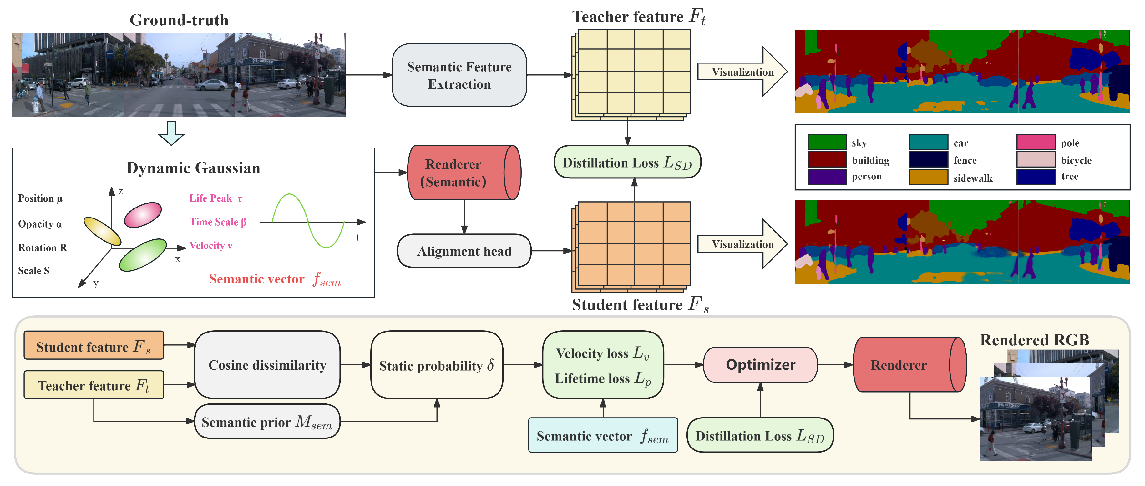
Figure 3.
Qualitative comparison results. The first two rows are from Waymo Open, and the last two rows are from KITTI. From left to right: Ground Truth, 3DGS, PVG, CoDa-4DGS, and SPT-Gauss.
Figure 3.
Qualitative comparison results. The first two rows are from Waymo Open, and the last two rows are from KITTI. From left to right: Ground Truth, 3DGS, PVG, CoDa-4DGS, and SPT-Gauss.
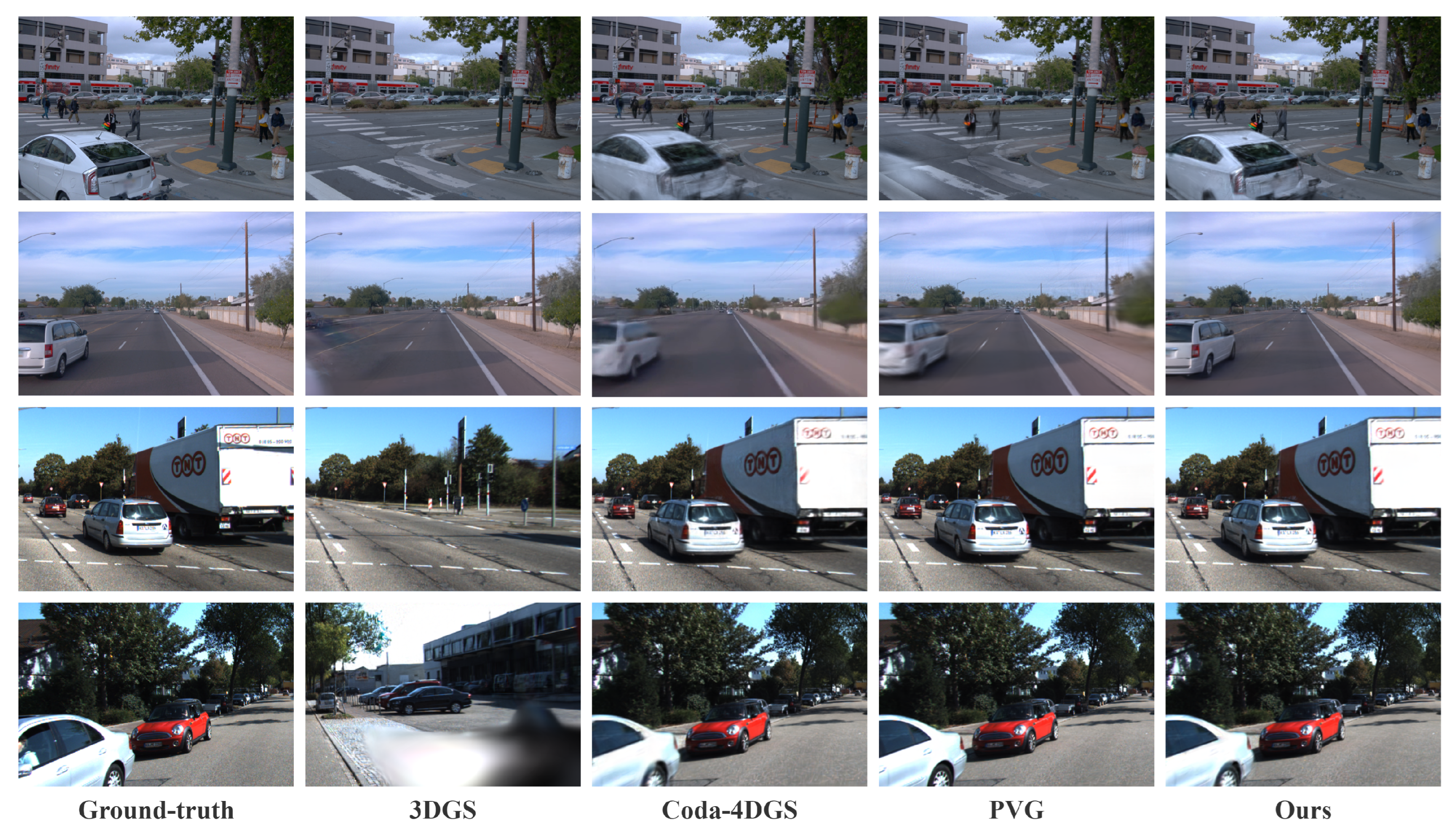
Figure 4.
Comparison of dynamic and static decomposition. The first column shows the ground truth (top) and the full reconstruction of SPT-Gauss (bottom). The remaining columns show decomposition results of PVG and SPT-Gauss, where the top and bottom rows represent dynamic and static components, respectively.
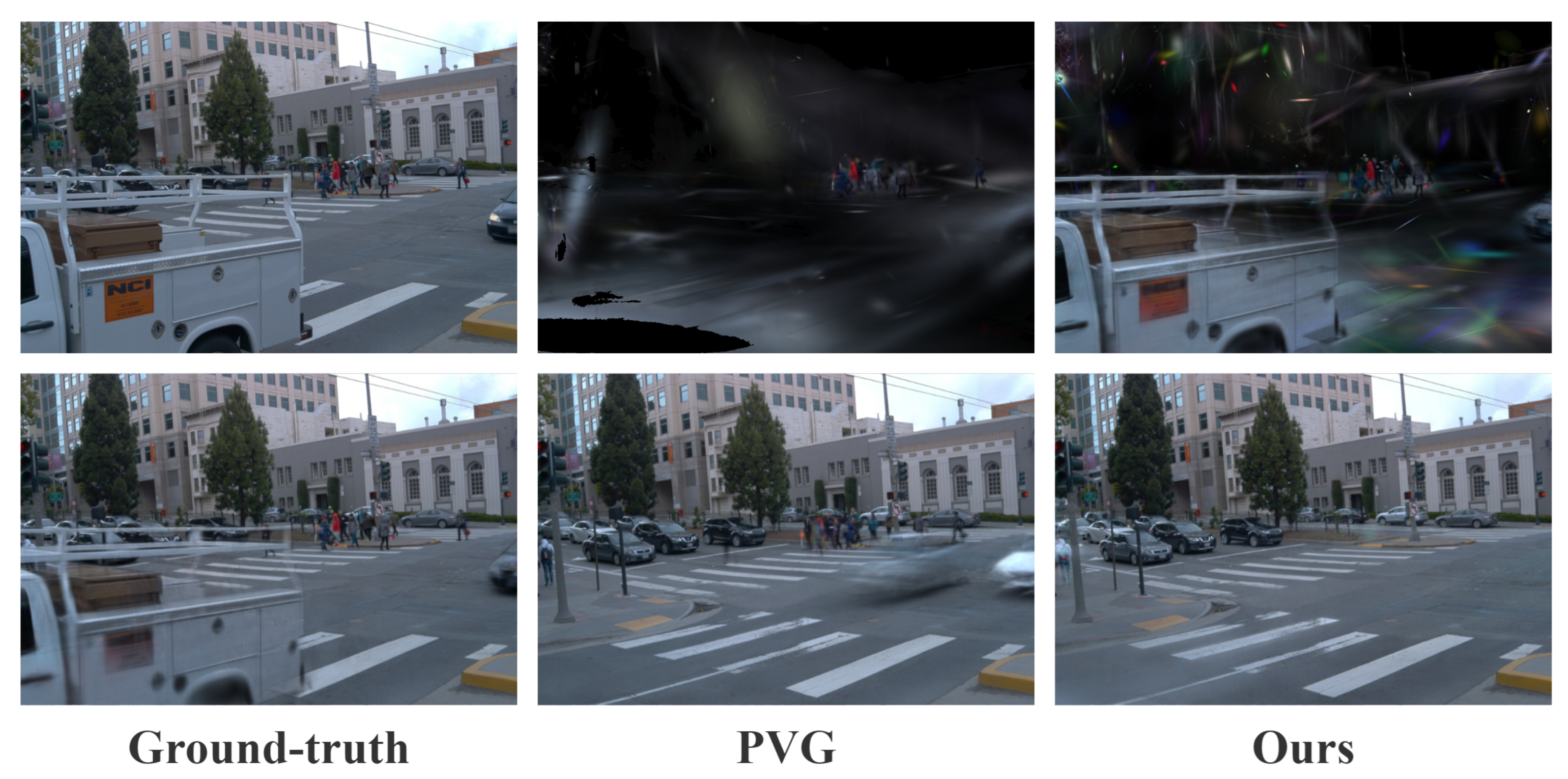
Figure 5.
Motion-mask comparison with and without semantic distillation (SD). The first column shows the ground truth; the next two columns correspond to results without SD (w/o SD) and with SD (w/ SD), respectively.
Figure 5.
Motion-mask comparison with and without semantic distillation (SD). The first column shows the ground truth; the next two columns correspond to results without SD (w/o SD) and with SD (w/ SD), respectively.
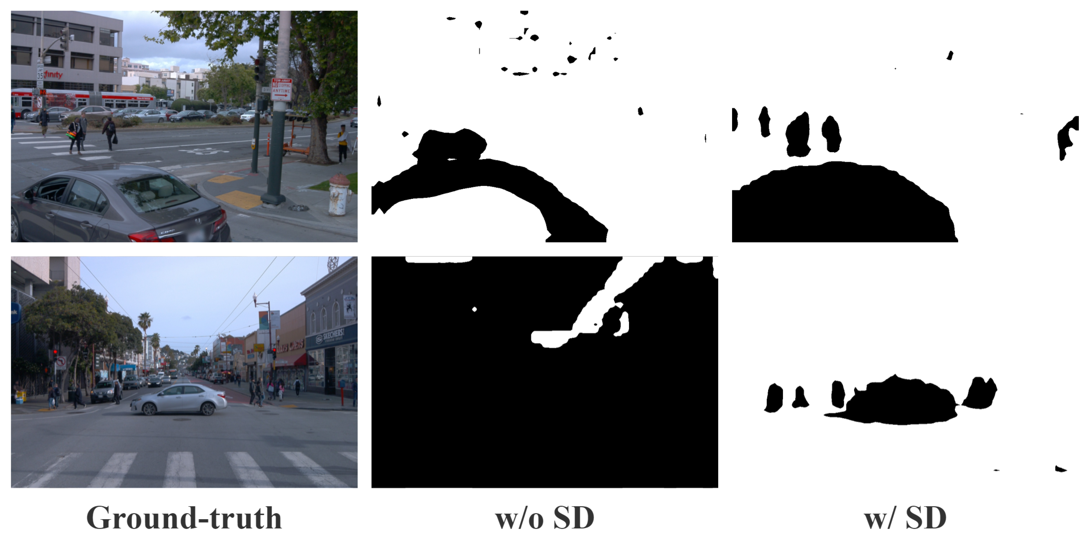

Table 1.
Quantitative comparison on Waymo Open and KITTI under the main comparison protocol. We report 4D reconstruction and NVS performance. Higher is better for PSNR/SSIM (↑); lower is better for LPIPS (↓).
Table 1.
Quantitative comparison on Waymo Open and KITTI under the main comparison protocol. We report 4D reconstruction and NVS performance. Higher is better for PSNR/SSIM (↑); lower is better for LPIPS (↓).
| Method | Waymo Open 4D Reconstruction |
Waymo Open NVS |
KITTI 4D Reconstruction |
KITTI NVS |
||||||||
|---|---|---|---|---|---|---|---|---|---|---|---|---|
| PSNR (↑) | SSIM (↑) | LPIPS (↓) | PSNR (↑) | SSIM (↑) | LPIPS (↓) | PSNR (↑) | SSIM (↑) | LPIPS (↓) | PSNR (↑) | SSIM (↑) | LPIPS (↓) | |
| 3DGS [6] | 27.99 | 0.866 | 0.293 | 25.08 | 0.822 | 0.319 | 21.02 | 0.811 | 0.202 | 19.54 | 0.776 | 0.224 |
| StreetSurf [42] | 26.70 | 0.846 | 0.372 | 23.78 | 0.822 | 0.401 | 24.14 | 0.819 | 0.257 | 22.48 | 0.763 | 0.304 |
| EmerNeRF [27] | 28.11 | 0.786 | 0.373 | 25.92 | 0.763 | 0.384 | 26.95 | 0.828 | 0.218 | 25.24 | 0.801 | 0.237 |
| SUDS [39] | 28.83 | 0.805 | 0.317 | 25.36 | 0.783 | 0.384 | 28.83 | 0.917 | 0.147 | 26.07 | 0.797 | 0.131 |
| MARS [43] | 21.81 | 0.681 | 0.430 | 20.69 | 0.636 | 0.453 | 27.96 | 0.900 | 0.185 | 24.31 | 0.845 | 0.160 |
| CoDa-4DGS [26] | 30.16 | 0.898 | 0.240 | 26.04 | 0.857 | 0.269 | 30.53 | 0.926 | 0.095 | 25.48 | 0.871 | 0.142 |
| PVG [17] | 32.46 | 0.910 | 0.229 | 28.11 | 0.849 | 0.279 | 32.83 | 0.937 | 0.070 | 27.43 | 0.879 | 0.114 |
| SPT-Gauss (Ours) | 34.12 | 0.926 | 0.189 | 30.23 | 0.905 | 0.197 | 34.50 | 0.955 | 0.057 | 29.80 | 0.903 | 0.108 |
Table 2.
Performance on dynamic regions of Waymo Open under the main comparison protocol. Region-wise scores are computed using ground-truth camera segmentation masks provided by Waymo (evaluated on labeled frames only).
Table 2.
Performance on dynamic regions of Waymo Open under the main comparison protocol. Region-wise scores are computed using ground-truth camera segmentation masks provided by Waymo (evaluated on labeled frames only).
| Method | D-PSNR (↑) | D-SSIM (↑) |
|---|---|---|
| 3DGS [6] | 18.65 | 0.803 |
| EmerNeRF [27] | 24.56 | 0.819 |
| CoDa-4DGS [26] | 26.08 | 0.871 |
| PVG [17] | 27.60 | 0.862 |
| SPT-Gauss (Ours) | 30.82 | 0.921 |
Table 3.
Ablation on Waymo Open under the ablation protocol (reduced subset). Absolute values are not directly comparable to Table 1.
Table 3.
Ablation on Waymo Open under the ablation protocol (reduced subset). Absolute values are not directly comparable to Table 1.
| Setting | PSNR | SSIM | LPIPS | D-PSNR | D-SSIM |
|---|---|---|---|---|---|
| w/o SD | 33.28 | 0.956 | 0.072 | 32.89 | 0.951 |
| w/o DEMM | 34.20 | 0.965 | 0.066 | 33.80 | 0.958 |
| w/o SVC | 35.02 | 0.969 | 0.066 | 34.22 | 0.966 |
| w/o SLP | 35.28 | 0.969 | 0.062 | 34.45 | 0.967 |
| Full | 35.54 | 0.971 | 0.060 | 34.63 | 0.970 |
Disclaimer/Publisher’s Note: The statements, opinions and data contained in all publications are solely those of the individual author(s) and contributor(s) and not of MDPI and/or the editor(s). MDPI and/or the editor(s) disclaim responsibility for any injury to people or property resulting from any ideas, methods, instructions or products referred to in the content. |
© 2026 by the authors. Licensee MDPI, Basel, Switzerland. This article is an open access article distributed under the terms and conditions of the Creative Commons Attribution (CC BY) license (http://creativecommons.org/licenses/by/4.0/).
Copyright: This open access article is published under a Creative Commons CC BY 4.0 license, which permit the free download, distribution, and reuse, provided that the author and preprint are cited in any reuse.


