
Submitted:
03 February 2026
Posted:
06 February 2026
You are already at the latest version
Abstract
Real-time monitoring of key parameters (e.g., substrate) is crucial for the precise control of biological fermentation processes. To address the technical bottlenecks of significant lag in offline analysis and the limitations of traditional online sensors, this study de-signed and implemented a universal AI-enabled electronic nose system. The system features a modular hardware architecture integrating a high-sensitivity MOS gas sensor array, a precision constant-temperature chamber, and low-noise signal acquisition circuits to ensure signal stability. On the software side, a software architecture was designed based on the RUP 4+1 view model, employing multi-threaded technology for parallel data processing. An innovative five-stage sampling period was designed to match the dynamic response of MOS sensors, facilitating reliable data acquisition. Combined with a truncated average filtering strategy and peak response feature ex-traction, a lightweight single-hidden-layer neural network model was constructed for real-time prediction. Taking the real-time prediction of methanol concentration during glucoamylase fermentation by Pichia pastoris as a case study, the system demonstrated outstanding performance: R² reached 0.9998, RMSE was 13.5326 ppm, and the prediction delay was less than 1 second. The proposed system provides a robust, efficient, and universally applicable hardware-software solution, demonstrating significant potential for intelligent biomanufacturing.
Keywords:
AI-enabled electronic nose
; biological fermentation
; real-time
; system design
; hardware integration
; software architecture
; neural network
1. Introduction
Biological fermentation technology is a core supporting technology in pharmaceuticals, food fermentation, bioenergy, and fine chemicals. The stability and optimization of fermentation processes directly determine the yield, purity, and production efficiency of the product. Precision control of these processes relies on real-time, accurate monitoring of multidimensional key parameters, including physical (e.g., temperature, pH), chemical (e.g., substrate concentration, dissolved oxygen), and biological parameters (e.g., cell density, metabolic activity) [1]. However, the industry faces two major technical challenges: First, traditional offline detection methods (e.g., GC-MS) are accurate but time-consuming, leading to significant lag that cannot meet real-time control. Second, conventional online sensors are primarily limited to basic physicochemical parameters, while critical metabolic intermediates (e.g., inducer concentrations) lack robust online detection due to complex industrial environments and interference factors [2,3]. This technological gap impedes real-time understanding of process states, restricting closed-loop optimization and intelligent transformation of fermentation processes.
Electronic nose technology provides an innovative solution by sensing fermentation exhaust gases and decoding their mapping with key parameters to achieve soft measurement, enabling non-contact, real-time inference of the internal state of fermentation broth [4,5]. Compared to traditional methods, electronic noses offer advantages such as fast response and adaptability to industrial scenarios. In this study, we develop an AI-enabled electronic nose system with a universal software-hardware architecture for real-time prediction of key fermentation parameters. Using methanol concentration prediction in Pichia pastoris fermentation as a case study, we demonstrate the system’s robustness through modular design, structured sampling cycles, and a lightweight neural network model, validated by high accuracy (R2 = 0.9998) and low latency (<1 s). This work emphasizes practical applications in industrial fermentation, providing a scalable solution for real-time monitoring.
The core innovation and main contributions of this study are as follows:
- Proposed a tri-integrated collaborative design philosophy encompassing hardware-level anti-interference, lower-computer truncated average filtering, and a stable algorithm model to construct a universal hardware-software collaborative electronic nose system architecture that unifies robustness, real-time performance, and scalability.
- Innovatively designed a five-stage structured sampling cycle to accurately match the dynamic response characteristics of MOS sensors (“adsorption-stability-desorption”), optimizing the time window for feature extraction and enhancing the reliability and representational capability of the feature data.
- At the hardware level, a circular sensor chamber integrated with a temperature control module was designed to suppress environmental temperature interference through closed-loop temperature control. At the software level, the sensor peak response was selected as the core feature to construct a lightweight single-hidden-layer neural network model, thereby significantly reducing computational complexity while maintaining prediction accuracy and thus meeting the resource constraints of industrial field deployment.
- Taking the prediction of methanol concentration in Pichia pastoris fermentation as a case study, the advantages of the proposed system in prediction accuracy, real-time performance, robustness, etc., were comprehensively verified through system performance testing and comparative experiments, and its potential for universal application in different fermentation systems was clarified.
The organization of this paper is as follows: Section 2 elaborates on the overall architecture design, hardware module implementation, and software system development of the electronic nose system; Section 3 deeply analyzes the correlation mechanism between fermentation process parameters and exhaust gas components, optimizes feature selection strategies, and constructs and validates a lightweight neural network prediction model; Section 4 summarizes research results and outlines future directions.
2. System Design
2.1. Overall System Architecture
2.1.1. Architecture Design Philosophy
This system is designed with the core concepts of “universality, robustness, real-time performance, and automatic prediction”, aiming to provide a solution for monitoring key process parameters in industrial fermentation scenarios.
- Universality: The hardware adopts a modular design, supporting flexible expansion and replacement of sensor arrays; The software reserves rich configuration interfaces, allowing users to adjust sampling parameters, features, and algorithm models according to different fermentation scenarios without changing the core framework to meet different needs;
- Robustness: Through multi-level collaborative design of “hardware anti-interference (constant temperature chamber temperature control) + lower-computer preprocessing (truncated average filtering denoising) + algorithm stable model (peak feature screening anti-drift + regularization to improve neural network generalization ability)”, the stability of the system in complex industrial environments is improved;
- Real-time performance: Adopting the architecture mode of “real-time acquisition by lower-computer + parallel processing by upper-computer”, the lower-computer uses STM32F103VET6 microcontroller to be responsible for sensor driving, gas path control, and raw signal acquisition; The upper-computer adopts an industrial control computer and processes tasks such as data transmission, feature extraction, model prediction, and result visualization in parallel through multi-threaded technology. Combined with a dual serial high-speed communication protocol, it ensures that the entire process delay from signal acquisition to prediction result output is less than 1 second;
- Automatic prediction: realizing the full process automation of “ baseline calibration - sampling - signal preprocessing - feature extraction - model prediction - result output, “ without manual intervention. The predicted results can be fed back in real-time to the downstream control system, providing data support for closed-loop optimization of the fermentation process.
2.1.2. Architecture Composition
The overall system consists of three parts: the fermentation tank unit, the gas path control unit, and the core electronic nose unit. The specific architecture is shown in Figure 1, and the actual operating scenario is shown in Figure 2. Among them, the core electronic nose unit includes three major modules: upper-computer, lower-computer, and sensor chamber:
- Lower-computer (STM32F103VET6): responsible for low-level hardware control and data acquisition tasks, including driving a 16-channel MOS sensor array, controlling the on-off switching of gas path solenoid valves, acquiring raw sensor response signals, chamber temperature data, and environmental temperature and humidity data, and using a truncated average filtering method to preprocess and upload the average data to the upper-computer;
- Upper-computer (industrial control computer): runs customized measurement and control software developed based on C# language, with core functions including data reception and storage, real-time data visualization, feature extraction, model inference and prediction based on PyTorch framework, system parameter configuration, and control instruction issuance;
- Gas path control unit: composed of an exhaust gas collection cylinder, a clean air source, an oxygen source, a solenoid valve, and a flow control module. Through the timing logic control of the lower-computer, it realizes the automatic switching of fermentation exhaust gas, clean air, and oxygen, and adapts to the multi-stage requirements of the sampling cycle.
The dual serial communication mode is adopted between the upper and lower computers to achieve efficient and isolated transmission of instructions and data:
- COM1 port: Dedicated exclusively to sensor-related communication. The upper-computer issues commands to read sensor signals via COM1, and the lower-computer uploads the corresponding response data via COM1;
- COM2 port: Dedicated exclusively to system control and monitoring. The upper-computer issues commands via COM2 to switch gas lines, read chamber temperature, and read ambient temperature and humidity. The lower-computer responds to the gas path switching commands and uploads the corresponding monitoring data.
This dedicated channel design of “instruction issuance - data return” clarifies the collaborative logic between the upper and lower computers, effectively avoiding transmission conflicts of different types of data streams, thereby ensuring the stability and overall efficiency of the communication link.
2.1.3. Workflow
The system workflow operates on a core “baseline calibration-sampling-prediction” cycle, with the following specific steps:
- Initialize baseline calibration phase: Upon system startup, clean air is continuously flushed through the sensor chamber until the response values of all 16 MOS sensors stabilize at baseline levels (baseline fluctuation ≤ ±0.1%), completing the initial sensor calibration.
- Closed-loop “Baseline Calibration-Sampling-Prediction” Cycle: Following baseline calibration completion, the system enters a cyclically executed five-phase closed-loop cycle of “Baseline Calibration-Sampling-Prediction,” with the specific workflow illustrated in Figure 3:
- Clean Air Introduction Phase: Continuous clean air flow maintains sensor baseline stability. Concurrently, the upper-computer processes sensor data collected in the previous cycle, performs feature extraction and model prediction, outputs prediction results, and stores them.
- Oxygen Introduction Phase: The gas path switches to introduce oxygen, providing an adequate reaction environment for redox reactions between the sensor surface and reductive components in the fermentation tail gas to ensure response sensitivity.
- Stabilization Phase: Maintain the current gas pathway state to eliminate disturbances caused by pathway switching, ensuring repeatability of sensor responses;
- Sampling Phase: Switch the gas pathway to introduce fermentation tank tail gas into the sensor chamber. Sixteen-channel MOS sensors simultaneously collect response signals for tail gas components. Raw data undergoes preliminary filtering by the lower-computer before being uploaded in real-time to the upper-computer;
- End of Sampling Phase: Close the fermentation tail gas pathway and switch to clean air to purge the sensor chamber, promoting desorption and restoring the sensor to baseline levels to prepare for the next sampling cycle.
Through the “baseline calibration-sampling-prediction” design, each sampling cycle guarantees stable, repeatable response signals, providing a high-quality data foundation for subsequent feature extraction and model prediction.
2.2. Response Characteristics of MOS Gas Sensors
MOS gas sensors have become the core component for sensing VOCs in electronic nose systems due to their advantages of low cost, fast response, high sensitivity, and wide detection range [6]. Its working mechanism and dynamic response characteristics are the key theoretical basis for system sampling period design, signal processing, and model construction.
The core working principle of MOS sensors is [7]: in clean air, the metal oxide layer on the sensor surface adsorbs oxygen, forming adsorbed oxygen ions (O 2−, O −, etc.), resulting in the sensor resistance value being maintained at a high level; When the reducing gas (such as methanol vapor) in the fermentation exhaust comes into contact with the sensor surface, an oxidation-reduction reaction occurs, releasing free electrons and significantly reducing the sensor resistance value. The resistance change of the sensor is positively correlated with the target gas concentration. After being converted into a voltage signal by the signal conditioning circuit, indirect characterization of the target gas concentration can be achieved.
The dynamic response process of MOS sensors to target gases follows a three-stage law of “adsorption - reaction and resistance change - desorption and recovery”. The typical response curve is shown in Figure 4 [7,8,9]:
- Adsorption stage: The target gas molecules diffuse to the sensor surface and are adsorbed by the sensitive material;
- Reaction and resistance change stage: The adsorbed gas molecules undergo oxidation-reduction reactions with pre-adsorbed oxygen ions on the surface of metal oxides, causing significant and rapid changes in the sensor resistance value. When the surface reaction reaches dynamic equilibrium, the response value of the sensor will tend to stabilize, and the signal in this stable stage can most accurately reflect the gas concentration, which is the optimal interval for feature extraction;
- Desorption and recovery stage: After the target gas is removed, the reaction products desorb from the surface of the sensitive material under the action of clean air blowing and sensor operating temperature, and the surface state of the sensitive material gradually returns to the initial baseline level.
The five-stage structured sampling period designed in this system is based on the dynamic response characteristics mentioned above. By accurately controlling the time allocation of each stage, it ensures effective sampling during the stable stage of sensor response, and improves the reliability and representation ability of feature data.
2.3. Hardware System Implementation
The design goal of the hardware system is to ensure the consistency of sensor response, low noise characteristics of signal acquisition, and adaptability to industrial environments. It revolves around the three core requirements of “constant temperature control, low noise acquisition, and modular integration”. The hardware structure of the system is shown in Figure 5.
2.3.1. Core Hardware Selection
- Sensor array: A 16-channel Figaro TGS series MOS sensor array is selected, including multiple models such as TGS2602 and TGS813, to enhance the system’s ability to identify complex fermentation exhaust gases and anti-interference performance through cross-response characteristics. After the raw signal of the sensor is preprocessed by truncation average filtering in the lower-computer, random noise is effectively eliminated;
- Temperature control module: The sensor chamber integrates nickel chromium alloy heating wire (for temperature rise), DC brushless fan (for temperature uniformity), and DS18B20 digital temperature sensor (for temperature acquisition); Simultaneously configure environmental temperature and humidity sensors. The system adopts a switch closed-loop control strategy (when the chamber temperature is above 50.0+0.5 ℃, the heating circuit solenoid valve is closed; when it is below 50-0.5 ℃, the solenoid valve is opened), combined with environmental temperature and humidity data to assist in judgment, to achieve stable control of the chamber working temperature of 50 ± 0.5 ℃ and suppress the influence of environmental fluctuations;
- Controller and power module: The lower-computer core controller uses an STM32F103VET6 microcontroller to meet the requirements of multi-sensor data acquisition and peripheral control; The power module adopts a multi-channel voltage regulation design to provide a stable working voltage for each hardware unit.
2.3.2. Key Structural Design
- Sensor chamber: Made of circular stainless steel material, fermentation exhaust gas flows uniformly along the central circular channel, and 16 MOS sensors are evenly arranged on the inner wall to ensure that the gas concentration and flow rate in contact with each sensor are consistent, thereby improving the consistency of the array response.
- Gas system: Three solenoid valves are used to achieve automatic switching of fermentation exhaust gas, clean air, and oxygen pathways, which are precisely controlled by the lower-computer according to the sampling stage requirements; Integrate flow control valves in the gas circuit to regulate gas flow rate and ensure response repeatability.
- Modular integration: The hardware system adopts a modular design and is integrated into a standard industrial chassis, which is easy to install and maintain, and improves anti-interference ability and mechanical stability.
2.3.3. Circuit System Design
- Signal conditioning circuit: The resistance change of the MOS sensor is converted into an analog voltage signal through a voltage divider sensing circuit (as shown in Figure 6 (a)). The lower-computer preprocesses each signal using the truncated average filtering method, collects 20 sets of raw data at a time, removes 2 maximum values and 2 minimum values, calculates the average value, and filters out instantaneous peak noise;
- Constant temperature control circuit: based on closed-loop feedback to achieve constant temperature control. Based on the real-time feedback provided by the temperature detection circuit (principle shown in Figure 6 (b)), adjust the working status of the heating wire and fan to achieve constant temperature control of the chamber at 50 ± 0.5 ℃;
- Communication circuit: Adopting a dual serial port independent communication mode, the two communication links work independently, effectively avoiding signal crosstalk.
2.4. Software System Design
This study adopts the RUP 4+1 view model and systematically models the software architecture using Rational Rose 7.0 [10,11,12,13]. The overall framework and the correlation logic between each view are shown in Figure 7.
2.4.1. Use Case View
The use case view defines the core functional modules and user interaction relationships of the system, where the core participants are experimental operators.
The core use cases include:
- Project management: creating, opening, saving, and exiting projects;
- Parameter configuration: setting the constant temperature value of the chamber, the duration of each stage of the sampling period, etc;
- Equipment testing: self-inspection and fault diagnosis of hardware devices such as sensor arrays, solenoid valves, heating wires, etc;
- Real-time monitoring: real-time collection and visualization of sensor response data, environmental temperature and humidity, and chamber temperature;
- Feature extraction: automatic extraction of features such as peak value, peak time, and area under the curve based on sensor response signals;
- Model prediction: call pre-trained neural network models to complete real-time prediction, output prediction results, and visualize them.
The experimental operator triggers the above use case through a graphical interface, and the interaction relationship is shown in Figure 8 (a).
2.4.2. Design View
Design views describe the static structure of software systems through package diagrams and class diagrams
- Package diagram: Divide the software system into functional modules such as project management, equipment testing, sampling period, chamber temperature, environmental temperature and humidity, model recognition, data visualization and storage, parameter configuration, and basic services, and clarify responsibilities and dependencies, as shown in Figure 8 (b);
- Class diagram: Define the core classes, properties, methods, and inter-class relationships of each module, as shown in Figure 8 (c).
2.4.3. Interactive View
The interactive view mainly solves the problems of concurrent execution and temporal interaction in the system, using multi-threading technology to achieve multi-task parallel processing. Scheduling serial port resources through a multi-threaded synchronization mechanism (mutex lock) to avoid thread resource preemption and data transmission conflicts, ensuring system real-time performance and stability. The core threads include:
- Sampling cycle thread: real-time display of the current sampling stage, model prediction of methanol concentration in the clean air introduction stage, and output of the results;
- Temperature and humidity monitoring thread: receive real-time chamber temperature, environmental temperature, and humidity data uploaded from the lower-computer, complete data analysis, visualization, and display;
- Sensor data thread: receive real-time sensor response data preprocessed by the lower-computer, perform data parsing, enable real-time visualization, and store historical data.
2.4.4. Implementing Views
The organization and relationship of software functional components are described in the implementation view. The core components include project management, temperature and humidity management, sampling period, testing equipment, pattern recognition, parameter settings, data visualization, and basic services. The component structure is shown in Figure 9.
2.4.5. Deployment View
The deployment view specifies the distributed deployment scheme of software functions on hardware nodes [11], as shown in Figure 10 (a):
- Lower-computer deployment: Develop embedded programs based on the C language to achieve underlying functions such as sensor driving, gas path control, temperature and humidity acquisition, constant temperature control, preliminary data filtering, and serial communication;
- Upper-computer deployment: Develop a graphical human-computer interaction interface based on C # language on the Visual Studio 2010 platform, integrating data reception, processing, visualization, and system configuration functions; Model training and prediction are implemented based on PyTorch and Scikit learn frameworks, using the ProcessStartInfo class in C # to call Python scripts to complete model prediction and achieve cross language collaborative reasoning.
The actual operating interface of the upper-computer is shown in Figure 10 (b), which mainly includes four functional areas: sampling process display area, real-time data display area, environmental parameter display area, and prediction result display area. The interface design is simple and intuitive, meeting the real-time monitoring and operation needs of experimental operators.
3. Feature Selection Strategy and Lightweight Neural Network Model Construction
Based on the dynamic response characteristics of MOS gas sensors in Section 2.2 and the feature extraction interface design of software systems in Section 2.4, this section further analyzes the correlation mechanism between fermentation process parameters and exhaust gas components, optimizes feature selection strategies, and constructs a prediction model.
3.1. Correlation Mechanism Between Process Parameters and Fermentation Exhaust Gas
During the process of biological fermentation, the growth and metabolic activities of bacterial cells follow a typical growth cycle pattern (lag period, exponential growth period, stable period, and decay period) [14,15,16,17]. At different growth stages, there are significant differences in the metabolic activity, nutrient consumption, and product synthesis rate of bacterial cells, which directly lead to periodic changes in the composition and concentration of VOCs in fermentation exhaust gas. This stage-specific VOCs release profile constitutes a unique ‘fingerprint’ of the fermentation process. The electronic nose captures this’ fingerprint ‘information and establishes a quantitative relationship with key parameters in the fermentation broth, such as inducer concentration, providing a theoretical basis for soft sensing of fermentation process parameters.
Existing studies have confirmed [18,19,20,21,22,23,24,25,26] that there is a correlation between some key process parameters in the fermentation broth (such as substrate methanol concentration) and the corresponding volatile component concentrations in the fermentation exhaust gas. For example, in the methanol-induced Pichia pastoris fermentation system, Ramon et al. achieved real-time estimation and control of methanol concentration in the fermentation broth by detecting the concentration of methanol vapor in the fermentation exhaust gas. This type of correlation mechanism originates from the mass transfer and phase equilibrium behavior between the liquid and gas phases in the fermentation system, providing a technical path and theoretical support for the development of soft sensing methods based on electronic noses.
3.2. Feature Selection Strategy
Static features (such as peak response Height), dynamic features (such as time-to-peak), and geometric features (such as area under the curve) can be extracted from the dynamic response curve of MOS sensors. Feature selection directly affects the prediction accuracy and robustness of the model.
Based on long-term experimental data and related literature [27], this study ultimately selected the peak response (Height) as the core feature parameter. The main reasons are as follows:
- Mechanism adaptability: The peak response of the sensor is strongly positively correlated with the target gas concentration, which is in line with the response mechanism of MOS sensors.
- Stability advantage: Compared to dynamic characteristics such as peak time that are easily affected by external factors, the response peak has stronger repeatability and better robustness between different periods.
- Strong characterization ability: The response peak can reflect the gas concentration intensity to the greatest extent possible, and the correlation with key parameters is significant.
To meet the scalability requirements, the software system has reserved interfaces for extracting features such as peak time and area under the curve.
3.3. Lightweight Neural Network Model Construction and Performance Evaluation
3.3.1. Model Construction Principle
Based on the universal approximation theorem [28,29,30,31], single hidden-layer feedforward neural networks can approximate continuous functions on compact sets with arbitrary accuracy, making them suitable for constructing complex mapping relationships between sensor response features and fermentation process parameters.
Model construction includes three key steps: data preparation, model structure design, and hyperparameter optimization:
3.3.2. Data Preparation
Owing to the significant challenges and high costs associated with acquiring large volumes of wide-range, precisely calibrated real-time methanol concentration data during actual fermentation processes, this study adopted a physics-informed data generation approach [32]. By inverting validated high-precision calibration equations—which encapsulate the well-established physical response characteristics of the MOS sensors—we were able to efficiently and controllably construct an initial dataset that covers the entire operational range. This strategy of integrating prior physical knowledge into the data generation process provides a reliable and cost-effective foundation for initial model training, especially in the early research phase.
The experimental dataset was generated by inverting the 11 MOS sensor ‘methanol concentration-response value’ one-quadratic calibration equations that have been validated in the literature [26] (the calibration equations all had a goodness of fit R2 > 0.98).
The data generation process is as follows:
- Concentration interval setting: with reference to the actual process requirements of glucoamylase production by Pichia pastoris fermentation, the sampling interval of methanol concentration is set at 100~2900 ppm, and 125 concentration points are uniformly selected within this interval.
- Response value calculation: Calculate the sensor response value corresponding to each concentration point through the calibration equation.
- Noise simulation: Add ± 1% Gaussian random noise to each response value to simulate industrial random interference.
- Dataset partitioning: The generated 125 samples will be randomly divided into a training set (100 groups) and a testing set (25 groups) in an 8:2 ratio for model training and performance evaluation.
It is important to note that while this physics-informed approach provides a robust and controllable dataset for initial model development, its ultimate validation will depend on future testing with real, long-term fermentation data to confirm its robustness against all potential environmental variabilities.
3.3.3. Model Structure Design
The model adopts a single hidden-layer feedforward neural network structure, and the specific design is as follows:
- Input layer: 11 neurons corresponding to the peak response characteristics of 11 sensors.
- Hidden layer: The number of neurons is determined through hyperparameter optimization using the ReLU activation function.
- Output layer: 1 neuron, corresponding to the predicted value of methanol concentration, using a linear activation function.
3.3.4. Hyperparameter Optimization
Model training and hyperparameter optimization were achieved through deep learning methods [33]: the Adam optimizer [34] was used for training, and grid search and 5-fold cross-validation strategies were combined to optimize hyperparameters [35]. The key hyperparameters and search range are as follows:
- Number of hidden layer neurons: [64,128];
- Learning rate: [0.02, 0.05];
- Learning rate decay coefficient (gamma): [0.8, 0.95];
- L2 regularization coefficient (l2_1ambda): [0.0005, 0.001, 0.005];
- Dropout probability: [0.1, 0.3];
- Patience value of early stopping method: [300,400,500].
To suppress model overfitting [36], a multiple regularization strategy is adopted:
- L2 regularization limits the weight scale by penalizing the sum of squares of the model’s weight parameters;
- Dropout reduces the model’s dependence on local features by randomly deactivating some neurons;
- The early stopping method monitors the validation set loss and stops training when the loss value no longer decreases for multiple epochs, avoiding overfitting caused by overtraining.
Through hyperparameter optimization, the optimal parameter configuration of the model is determined as follows: 64 hidden layer neurons, learning rate of 0.05, L2 regularization coefficient of 0.0005, Dropout probability of 0.1, and patience value of 400 for the early stopping method.
3.3.5. Model Performance Evaluation
The performance evaluation of the model is carried out from two dimensions: overall prediction accuracy and stability of concentration intervals, using determination coefficient (R2), RMSE, MAE, and prediction delay as core evaluation indicators.
3.3.5.1. Overall Performance
The overall performance metrics of the model on the training and testing sets are shown in Table 1. The test set R2 is as high as 0.9998, RMSE is 13.5326 ppm, MAE is 12.2667 ppm, and the predicted delay is only 0.8 seconds. The training loss curve rapidly decreases and tends to stabilize, and the difference between the predicted value and the true value is small (Figure 11), indicating that the model has good generalization ability and no overfitting phenomenon.
3.3.5.2. Performance in Concentration Range
To verify the stability of the model in different concentration ranges, the test set was divided into low (100-1000 ppm), medium (1000-2000 ppm), and high (2000-2900 ppm) concentration intervals for evaluation. The results are shown in Table 2 and Figure 12. The model maintains excellent performance in all regions, with R 2 higher than 0.997, RMSE less than 17.77 ppm, and MAE less than 15.58 ppm. The prediction accuracy is highest in the low concentration range (RMSE=11.2713 ppm, MAE=10.6508 ppm), while the prediction error slightly increases in the high concentration range due to the slight saturation of sensor response, but still meets application requirements.
3.3.6. Model Performance Comparison
To verify the superiority of the constructed lightweight neural network model, comparative experiments were conducted with support vector regression (SVR), random forest regression, and double hidden-layer fully connected neural networks (FCNN-2). All models use the same training and testing sets, and optimize hyperparameters through grid search combined with 5-fold cross-validation to ensure fairness in comparative experiments.
- Prediction accuracy: The lightweight neural network has comparable accuracy to FCNN-2 (R 2 is close to 0.999), significantly better than SVR and random forest.
- Model complexity: The lightweight neural network has only 833 parameters, which is much lower than the 4993 parameters of FCNN-2. It has higher computational efficiency and is more suitable for industrial scenarios with limited resources.
Overall, the lightweight neural networks have the advantages of fewer parameters and higher computational efficiency while ensuring high accuracy, which is more in line with industrial deployment requirements.
3.3.7. Model Deployment and Application Value
The optimized lightweight neural network model after training is deployed on the upper-computer system, encapsulated by Python scripts and called by C# upper-computer software to achieve automated inference. The deployment and operation process of the model is as follows:
- Data input: During the “clean air introduction” stage of the sampling cycle, the upper-computer automatically extracts the peak response characteristics of 11 sensors from the previous cycle.
- Model inference: Call the encapsulated PyTorch model to output the predicted methanol concentration value.
- Result output: The predicted results are displayed in real-time and can be transmitted to downstream fermentation control systems for closed-loop adjustment of process parameters.
This solution achieves full process automation operation, with a predicted delay of less than 1 second, and can meet the real-time regulation requirements during the stable fermentation period. The system can effectively avoid problems caused by high or low methanol concentration through real-time monitoring, providing key data support for closed-loop optimization of fermentation processes and having significant engineering application value.
4. Summary and Outlook
4.1. Research Summary
This study focuses on the real-time monitoring requirements of key parameters in the biological fermentation process, and successfully develops an AI-enabled electronic nose system for real-time prediction of biological fermentation parameters. The universal software and hardware architecture has been validated through typical cases. The core achievements are as follows:
- A three-in-one software-hardware collaborative architecture has been proposed, achieving the unity of universality, robustness, and real-time performance, laying the foundation for engineering applications and reuse.
- A multi-level anti-interference system has been constructed, which improves the stability of the system in complex industrial environments through hardware constant temperature control, lower-computer filtering preprocessing, and feature selection.
- Innovatively designed a five-stage structured sampling period to accurately match the dynamic characteristics of sensors; The lightweight neural network constructed ensures high accuracy (R 2=0.9998, RMSE=13.5326 ppm) while significantly reducing the number of parameters (833), with a prediction delay of less than 1 second.
- Through typical case verification, it has been demonstrated that the system has excellent prediction accuracy, real-time performance, robustness, and potential for universal application in different fermentation systems.
This study provides a reliable solution for reducing the uncertainty of the fermentation process and achieving intelligent biomanufacturing.
4.2. Future Research Directions
- Expand the scope of universal adaptation: Expand the types of sensor arrays (such as electrochemical and infrared sensors), explore multi-feature fusion strategies, and extend their application to predict more parameters, such as bacterial concentration and product concentration.
- Building a monitoring control closed-loop system: Combining predicted results with advanced process control algorithms to develop closed-loop optimization control strategies, achieving closed-loop upgrades from parameter monitoring to automatic adjustment, and enhancing the intelligence level of the fermentation process.
Author Contributions
Conceptualization, X.Z. and D.G.; methodology, X.Z. and D.G.; software, X.Z.; validation, X.Z. and D.G.; formal analysis, X.Z.; investigation, X.Z.; resources, D.G.; data curation, X.Z.; writing—original draft preparation, X.Z.; writing—review and editing, D.G.; visualization, X.Z.; supervision, D.G.; project administration, D.G.; funding acquisition, D.G. All authors have read and agreed to the published version of the manuscript.
Funding
This research received no external funding.
Institutional Review Board Statement
Not applicable.
Informed Consent Statement
Not applicable.
Data Availability Statement
The data that support the findings of this study are available from the corresponding author upon reasonable request.
Abbreviations
The following abbreviations are used in this manuscript:
| AI | Artificial Intelligence |
| MOS | Metal-Oxide Semiconductor |
| RMSE | Root Mean Square Error |
| GC-MS | Gas Chromatography - Mass Spectrometry |
| VOCs | Volatile Organic Compounds |
| RUP | Rational Unified Process |
| MAE | mean absolute error |
References
- Jaibiba, P.; Naga Vignesh, S.; Hariharan, S. Chapter 10 - Working principle of typical bioreactors. In Bioreactors; Singh, L., Yousuf, A., Mahapatra, D.M., Eds.; Elsevier: Amsterdam, The Netherlands, 2020; pp. 145–173. [Google Scholar] [CrossRef]
- Xia, J.; Long, D.; Chen, M.; Chen, A. Optimization of fermentation processes in intelligent biomanufacturing: on online monitoring, artificial intelligence, and digital twin technologies. Chinese Journal of Biotechnology 2025, 41, 1179–1196. [Google Scholar] [CrossRef]
- Palladino, F.; Marcelino, P.R.F.; Schlogl, A.E.; José, Á.H.M.; Rodrigues, R.d.C.L.B.; Fabrino, D.L.; Santos, I.J.B.; Rosa, C.A. Bioreactors: Applications and Innovations for a Sustainable and Healthy Future—A Critical Review. Appl. Sci 2024, 14, 9346. [Google Scholar] [CrossRef]
- Zhang, X.; Wang, T.; Ni, W.; Zhang, Y.; Lv, W.; Zeng, M.; Yang, J.; Hu, N.; Zhan, R.; Li, G.; et al. Sensor array optimization for the electronic nose via different deep learning methods. Sensors and Actuators B: Chemical 2024, 410, 135579. [Google Scholar] [CrossRef]
- Gardner, J.W.; Bartlett, P.N. A brief history of electronic noses. Sensors and Actuators B: Chemical 1994, 18, 210–211. [Google Scholar] [CrossRef]
- Ijaz, U.; Ali, M.; Ahmad, I.; Hamza, S.A.; Kim, H.D. A comprehensive review of electronic nose systems: design, sensors, and future directions. Chemical Engineering Journal 2025, 524, 169482. [Google Scholar] [CrossRef]
- Yuan, C.; Ma, J.; Zou, Y.; Li, G.; Xu, H.; Sysoev, V.V.; Cheng, X.; Deng, Y. Modeling Interfacial Interaction between Gas Molecules and Semiconductor Metal Oxides: A New View Angle on Gas Sensing. Advanced Science 2022, 9. [Google Scholar] [CrossRef]
- Zhao, H.; Wang, Y.; Zhou, Y. Accelerating the Gas–Solid Interactions for Conductometric Gas Sensors: Impacting Factors and Improvement Strategies. Materials 2023, 16. [Google Scholar] [CrossRef] [PubMed]
- Zhao, L.; Wang, X.; Zhang, Z.; Ji, Y.; Guo, J.; Du, Z.; Cheng, G. Realizing the Ultrafast Recovery of the Monolayer MoS2-Based NH3 Sensor by Gas-Ion-Gate. ACS Applied Materials & Interfaces 2025, 17, 17465–17475. [Google Scholar] [CrossRef]
- Booch, G.; Rumbaugh, J.; Jacobson, I. The Unified Modeling Language User Guide, 2nd ed.; Addison-Wesley: Upper Saddle River, NJ, 2005; pp. 14–34. [Google Scholar]
- Kruchten, P.B. The 4+1 View Model of architecture. IEEE Software 1995, 12, 42–50. [Google Scholar] [CrossRef]
- Pressman, R.; Maxim, B. Software Engineering: A Practitioner’s Approach, 9th ed.; McGraw-Hill Education: New York, USA, 2019; pp. 181–184. [Google Scholar]
- IEEE/ISO/IEC International Standard for Software, systems and enterprise--Architecture description. ISO/IEC/IEEE 42010 2022, (E) 2022, 1–74. [CrossRef]
- Monod, J. THE GROWTH OF BACTERIAL CULTURES. Annual Review of Microbiology 1949, 3, 371–394. [Google Scholar] [CrossRef]
- Madigan, M.T.; Bender, K.S.; Buckley, D.H.; Sattley, W.M.; Stahl, D.A. Brock Biology of Microorganisms, 16th ed.; Pearson: New York, USA, 2020; pp. 144–177. [Google Scholar]
- Bate, F.; Amekan, Y.; Pushkin, D.O.; Chong, J.P.J.; Bees, M. Emergent Lag Phase in Flux-Regulation Models of Bacterial Growth. B Math Biol 2023, 85. [Google Scholar] [CrossRef] [PubMed]
- Ardré, M.; Doulcier, G.; Brenner, N.; Rainey, P.B. A leader cell triggers end of lag phase in populations of Pseudomonas fluorescens. microLife 2022, 3, uqac022. [Google Scholar] [CrossRef] [PubMed]
- Ramon, R.; Feliu, J.; Cos, O.; et al. Improving the monitoring of methanol concentration during high cell density fermentation of Pichia pastoris. Biotechnology Letters 2004, 26, 1447–1452. [Google Scholar] [CrossRef]
- Guarna, M.M.; Lesnicki, G.J.; Tam, B.M.; et al. On-line monitoring and control of methanol concentration in shake-flask cultures of Pichia pastoris. Biotechnol Bioeng 1997, 56, 279–286. [Google Scholar] [CrossRef]
- Hellwig, S.; Emde, F.; Raven, N.P.; Henke, M.; van Der Logt, P.; Fischer, R. Analysis of single-chain antibody production in Pichia pastoris using on-line methanol control in fed-batch and mixed-feed fermentations. Biotechnol Bioeng 2001, 74, 344–352. [Google Scholar] [CrossRef]
- Seesaard, T.; Wongchoosuk, C. Recent Progress in Electronic Noses for Fermented Foods and Beverages Applications. Fermentation 2022, 8, 302. [Google Scholar] [CrossRef]
- Salgado, A.M.; Folly, R.O.M.; Valdman, B.; Valero, F. Model based soft-sensor for on-line determination of substrate. Applied Biochemistry and Biotechnology 2004, 113, 137–144. [Google Scholar] [CrossRef]
- Groboillot, A.; Pons, M.N.; Engasser, J.M. Influence of some fermentation medium components on the response of a gas membrane sensor for detection of volatiles. Bioprocess Engineering 1990, 5, 217–224. [Google Scholar] [CrossRef]
- Beuvink, J.M.W.; Spoelstra, S.F. Interactions between substrate, fermentation end-products, buffering systems and gas production upon fermentation of different carbohydrates by mixed rumen microorganisms in vitro. Applied Microbiology and Biotechnology 1992, 37, 505–509. [Google Scholar] [CrossRef]
- Yang, G.; Wang, J. Biohydrogen production by co-fermentation of sewage sludge and grass residue: Effect of various substrate concentrations. Fuel 2019, 237, 1203–1208. [Google Scholar] [CrossRef]
- Hui-lin, SHI; Jing-chun, SUN; Rong-kai, ZHANG; Da-qi, GAO; Ze-jian, WANG; Mei-jin, GUO; Li-qin, ZHOU; Ying-ping, ZHUANG. Application of the Electronic Nose on the Online Feedback Control of Methanol Concentration during Glucoamylase Fermentation Optimization by Pichia pastoris. China Biotechnology 2016, 36, 68–76. [Google Scholar]
- Anker, M.; Yousefi-Darani, A.; Zettel, V.; Paquet-Durand, O.; Hitzmann, B.; Krupitzer, C. Online Monitoring of Sourdough Fermentation Using a Gas Sensor Array with Multivariate Data Analysis. Sensors 2023, 23, 7681. [Google Scholar] [CrossRef] [PubMed]
- Cybenko, G. Approximation by superpositions of a sigmoidal function. Mathematics of Control, Signals and Systems 1989, 2, 303–314. [Google Scholar] [CrossRef]
- Hornik, K.; Stinchcombe, M.; White, H. Multilayer feedforward networks are universal approximators. Neural Networks 1989, 2, 359–366. [Google Scholar] [CrossRef]
- Funahashi, K.-I. On the approximate realization of continuous mappings by neural networks. Neural Networks 1989, 2, 183–192. [Google Scholar] [CrossRef]
- Chong, K.F.E. A closer look at the approximation capabilities of neural networks. ArXiv 2020. abs/2002.06505. [Google Scholar]
- Karniadakis, G.E.; Kevrekidis, I.G.; Lu, L.; Perdikaris, P.; Wang, S.F.; Yang, L. Physics-informed machine learning. Nat Rev Phys 2021, 3, 422–440. [Google Scholar] [CrossRef]
- LeCun, Y.; Bengio, Y.; Hinton, G. Deep learning. Nature 2015, 521, 436–444. [Google Scholar] [CrossRef]
- Kingma, Diederik P.; Ba, Jimmy. Adam: A Method for Stochastic Optimization. In Proceedings of the 3rd International Conference on Learning Representations (ICLR), San Diego, CA, USA, 2015. [Google Scholar]
- Bergstra, J.; Bengio, Y. Random Search for Hyper-Parameter Optimization. J Mach Learn Res 2012, 13, 281–305. [Google Scholar]
- Srivastava, N.; Hinton, G.; Krizhevsky, A.; Sutskever, I.; Salakhutdinov, R. Dropout: A Simple Way to Prevent Neural Networks from Overfitting. J Mach Learn Res 2014, 15, 1929–1958. [Google Scholar]
Figure 1.
Overall architecture diagram of the electronic nose system.
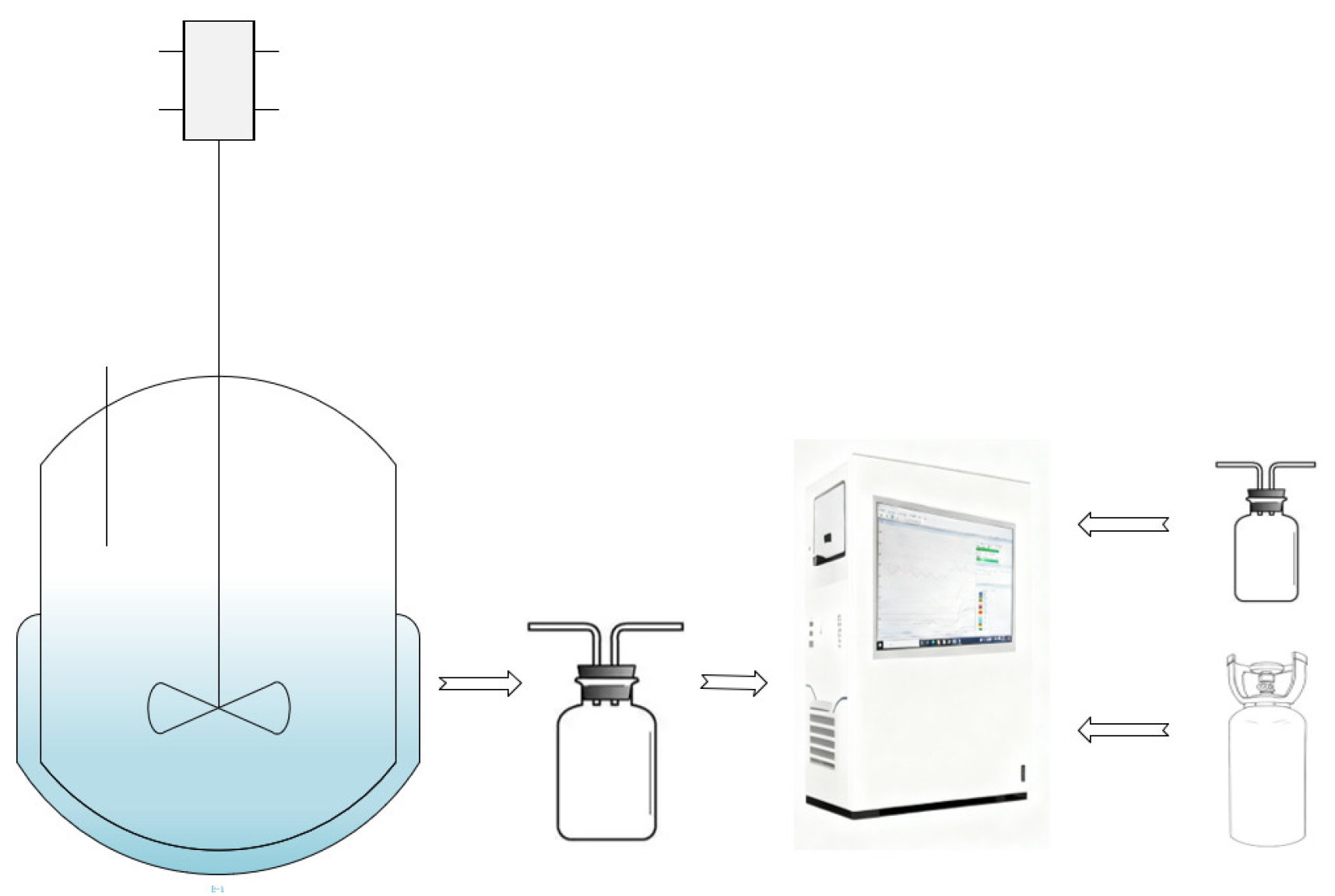
Figure 2.
Realistic Operation Scene of Electronic Nose System.
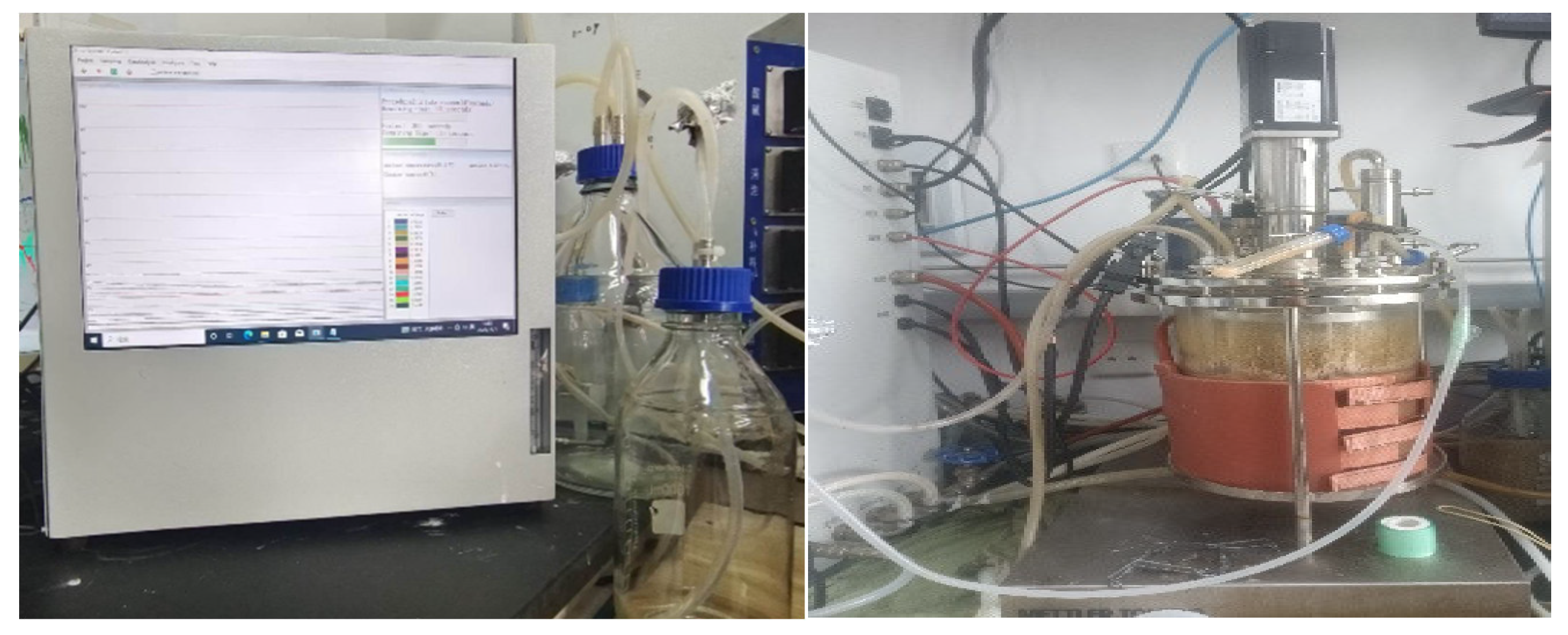
Figure 3.
Workflow diagram of the electronic nose system.
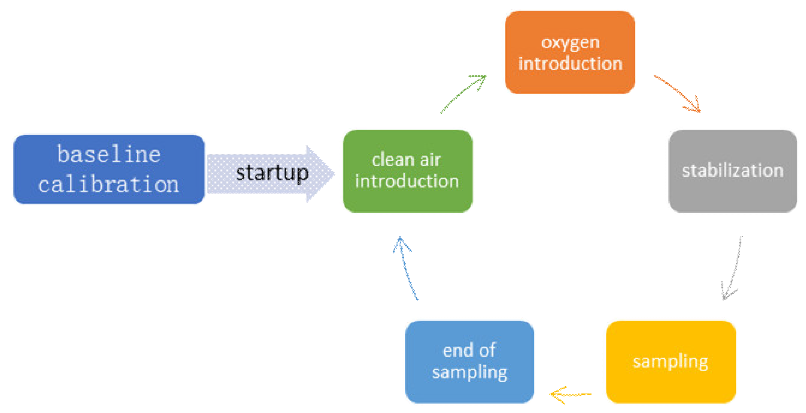
Figure 4.
Dynamic Response Curve of MOS Gas Sensor: “Adsorption–Reaction and Resistance Change–Desorption and Recovery”.
Figure 4.
Dynamic Response Curve of MOS Gas Sensor: “Adsorption–Reaction and Resistance Change–Desorption and Recovery”.
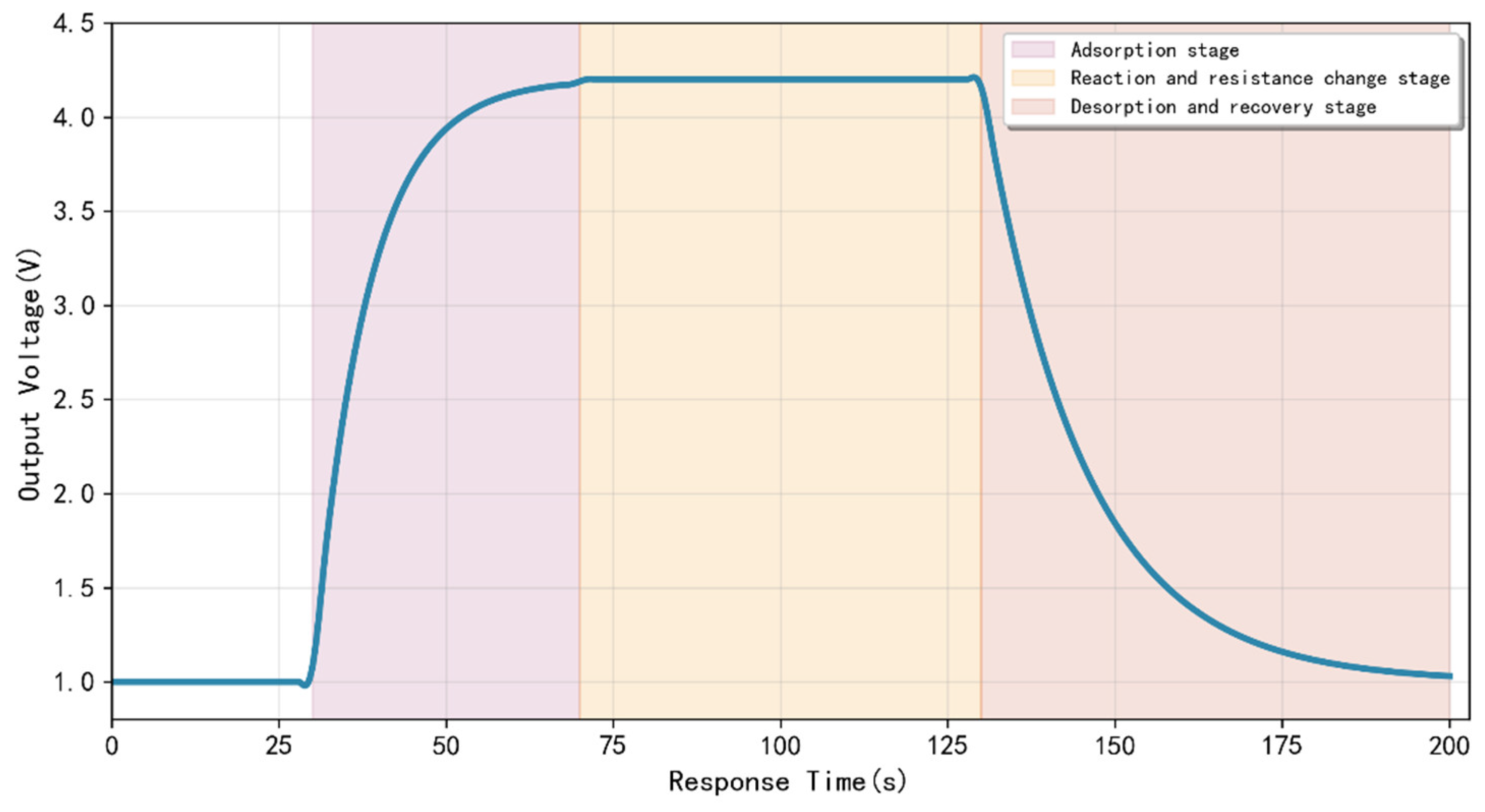
Figure 5.
Hardware Structure Diagram.
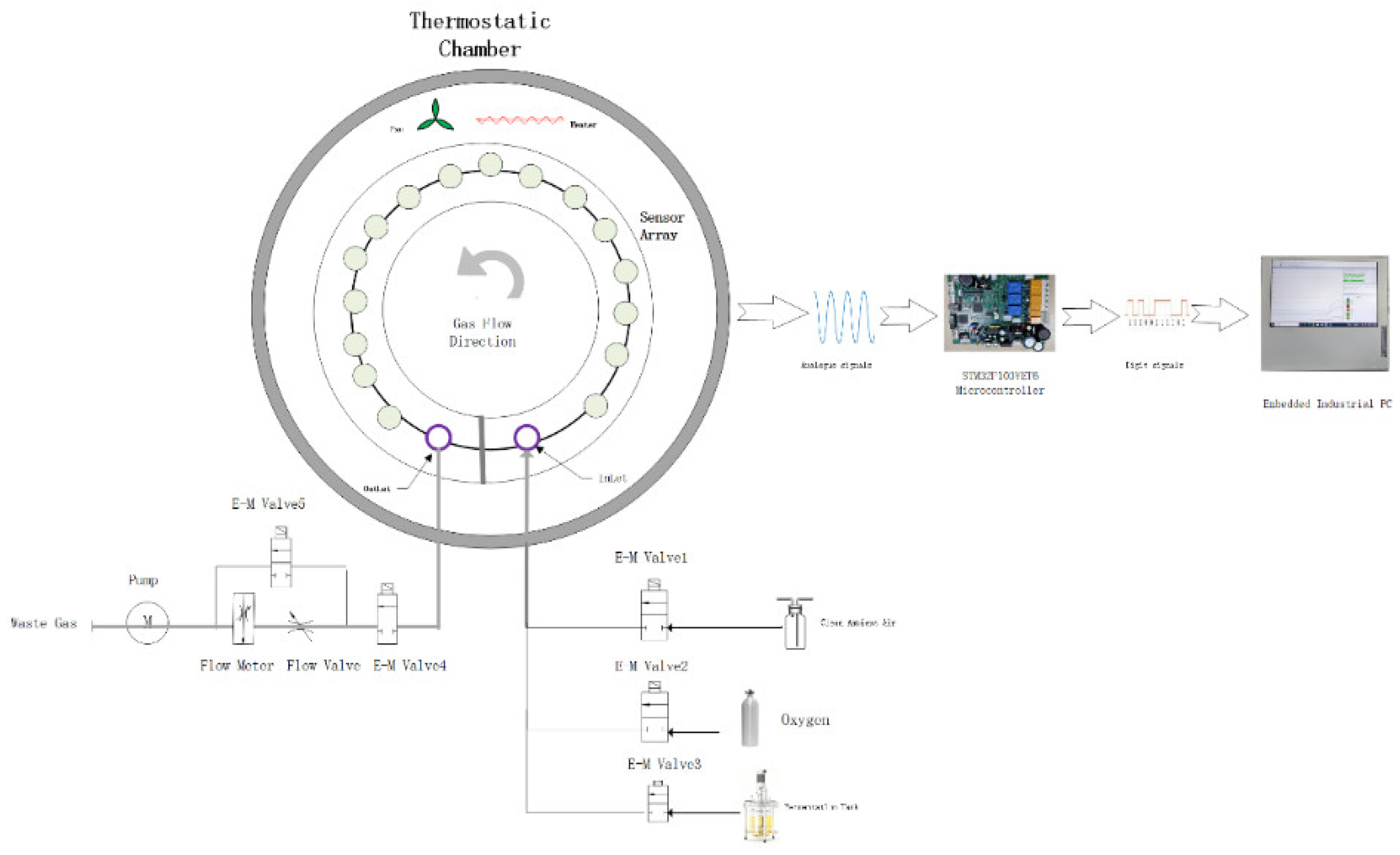
Figure 6.
Circuit system design (a) Schematic diagram of voltage divider sensing circuit; (b) Schematic diagram of temperature detection circuit.
Figure 6.
Circuit system design (a) Schematic diagram of voltage divider sensing circuit; (b) Schematic diagram of temperature detection circuit.
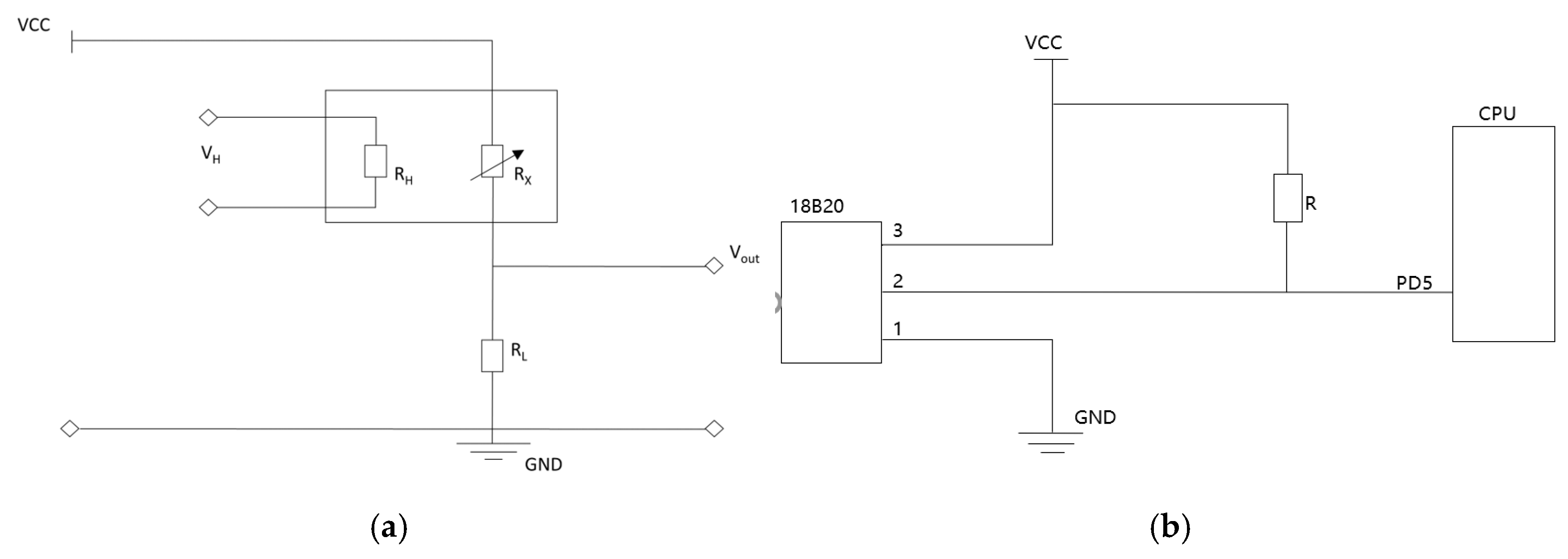
Figure 7.
RUP 4+1 View Model.
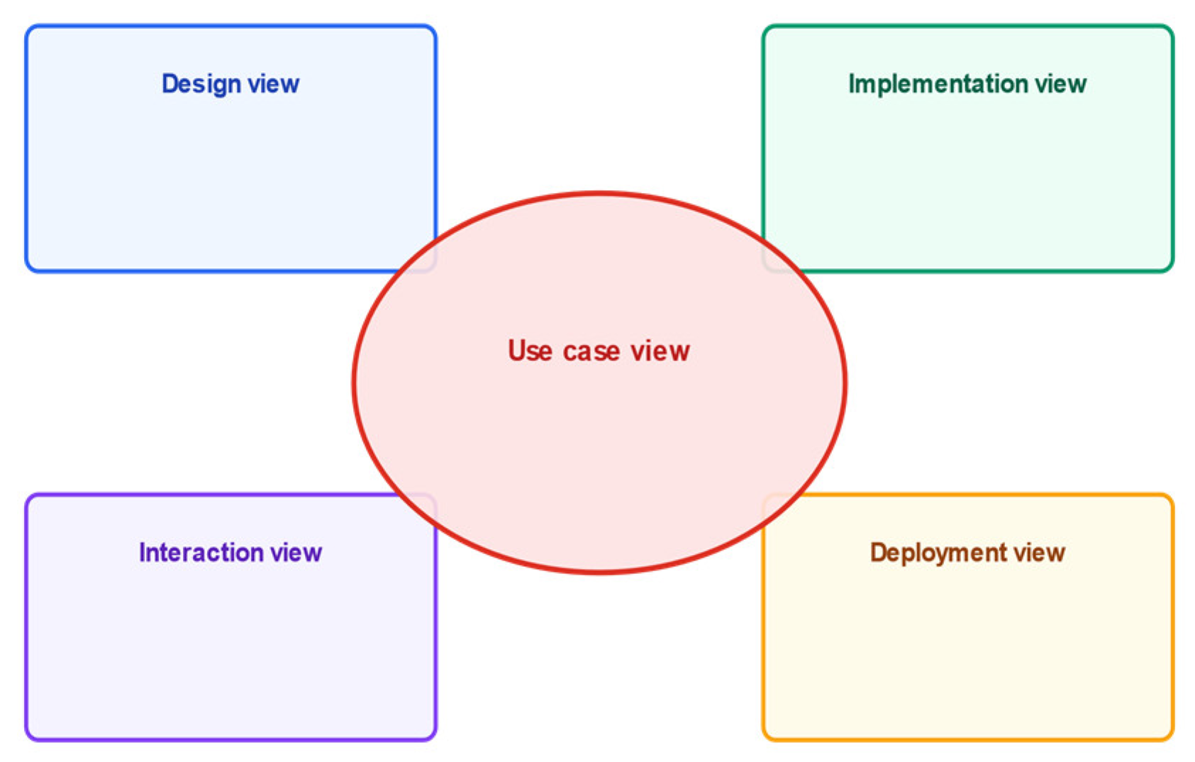
Figure 8.
UML diagrams of the use case view and design view. (a) Use case diagram; (b) Package diagram; (c) Class diagram.
Figure 8.
UML diagrams of the use case view and design view. (a) Use case diagram; (b) Package diagram; (c) Class diagram.
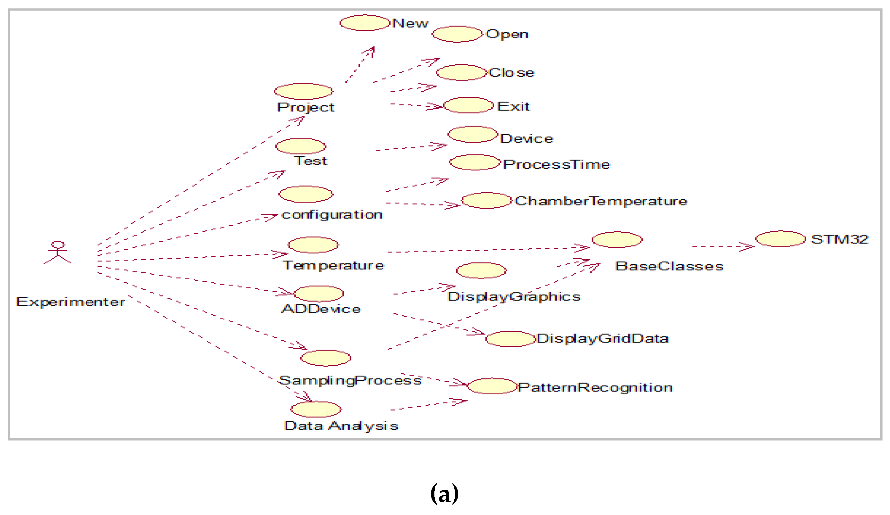

Figure 9.
Component diagram of the implementation view.
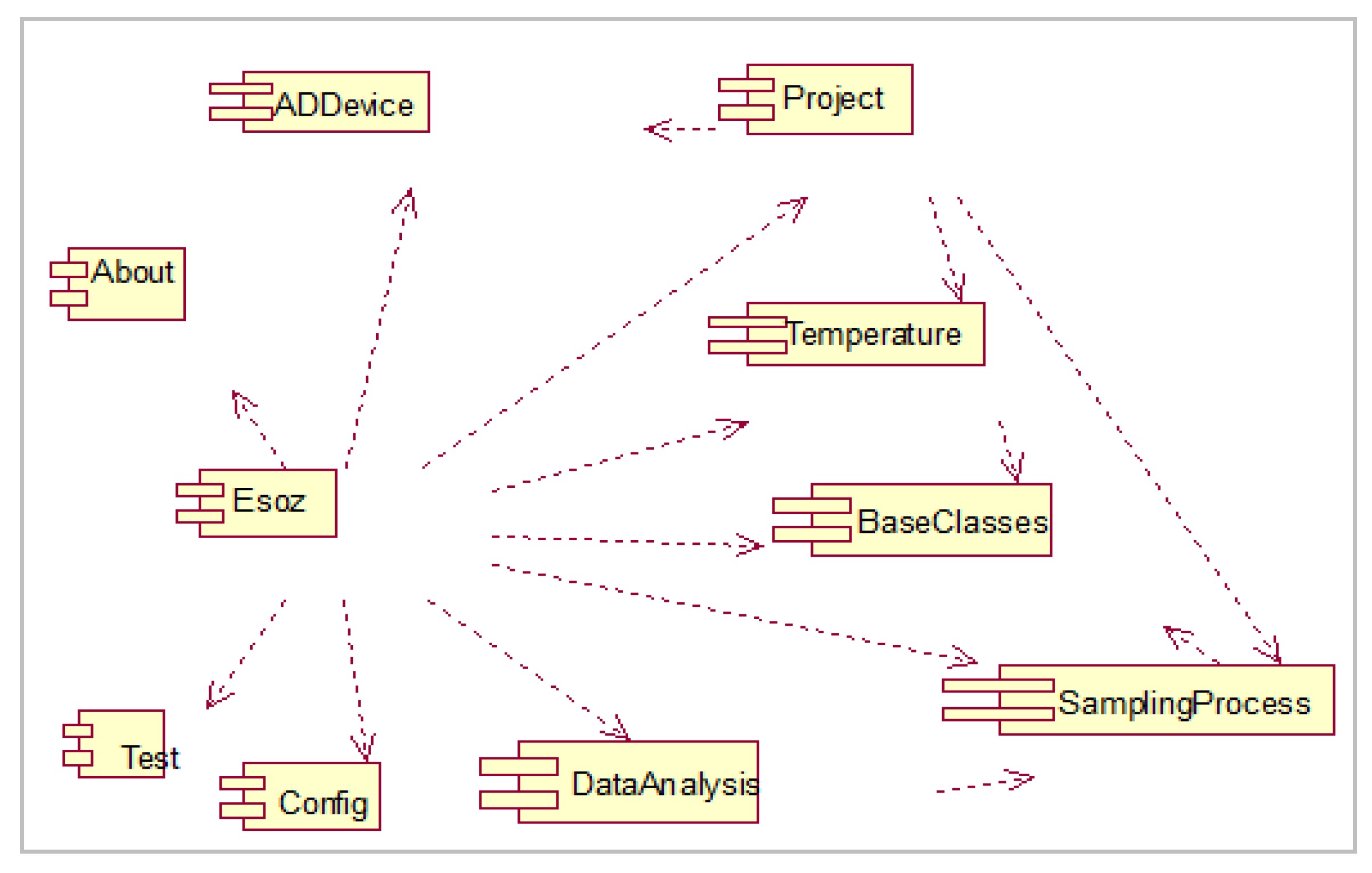
Figure 10.
Deployment diagram and upper-computer running interface. (a) Deployment diagram; (b) Screenshot of the upper-computer running interface.
Figure 10.
Deployment diagram and upper-computer running interface. (a) Deployment diagram; (b) Screenshot of the upper-computer running interface.
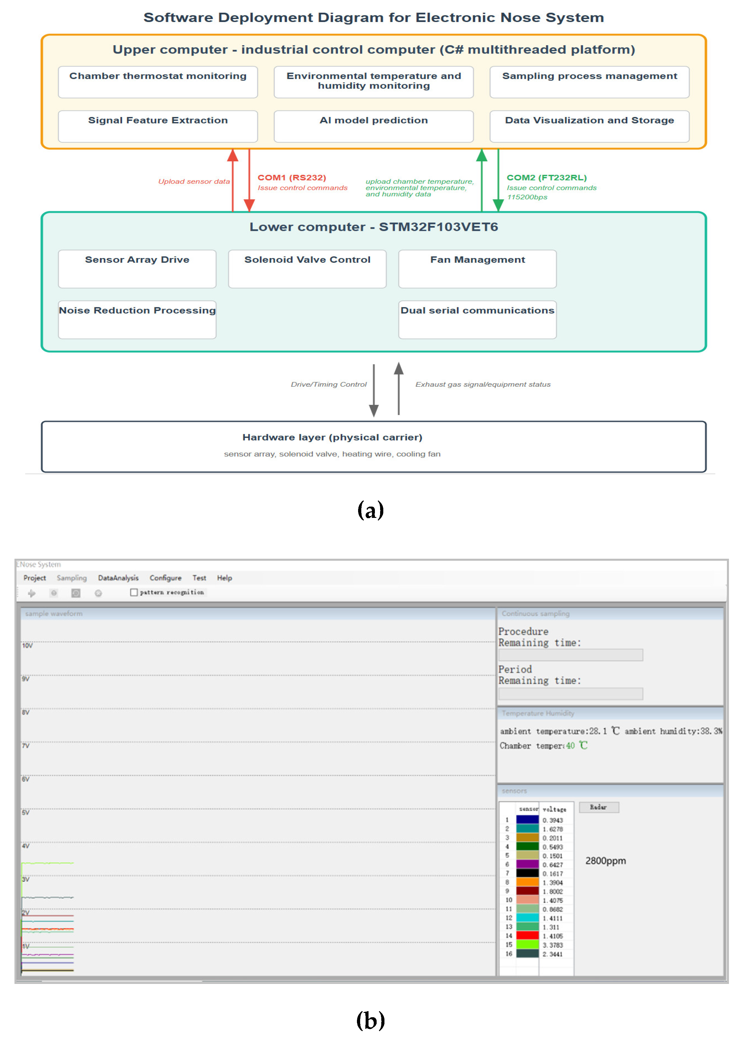
Figure 11.
Overall performance verification results of the model (a) Comparison chart of predicted and true values in the training/testing set; (b) Training loss curve.
Figure 11.
Overall performance verification results of the model (a) Comparison chart of predicted and true values in the training/testing set; (b) Training loss curve.
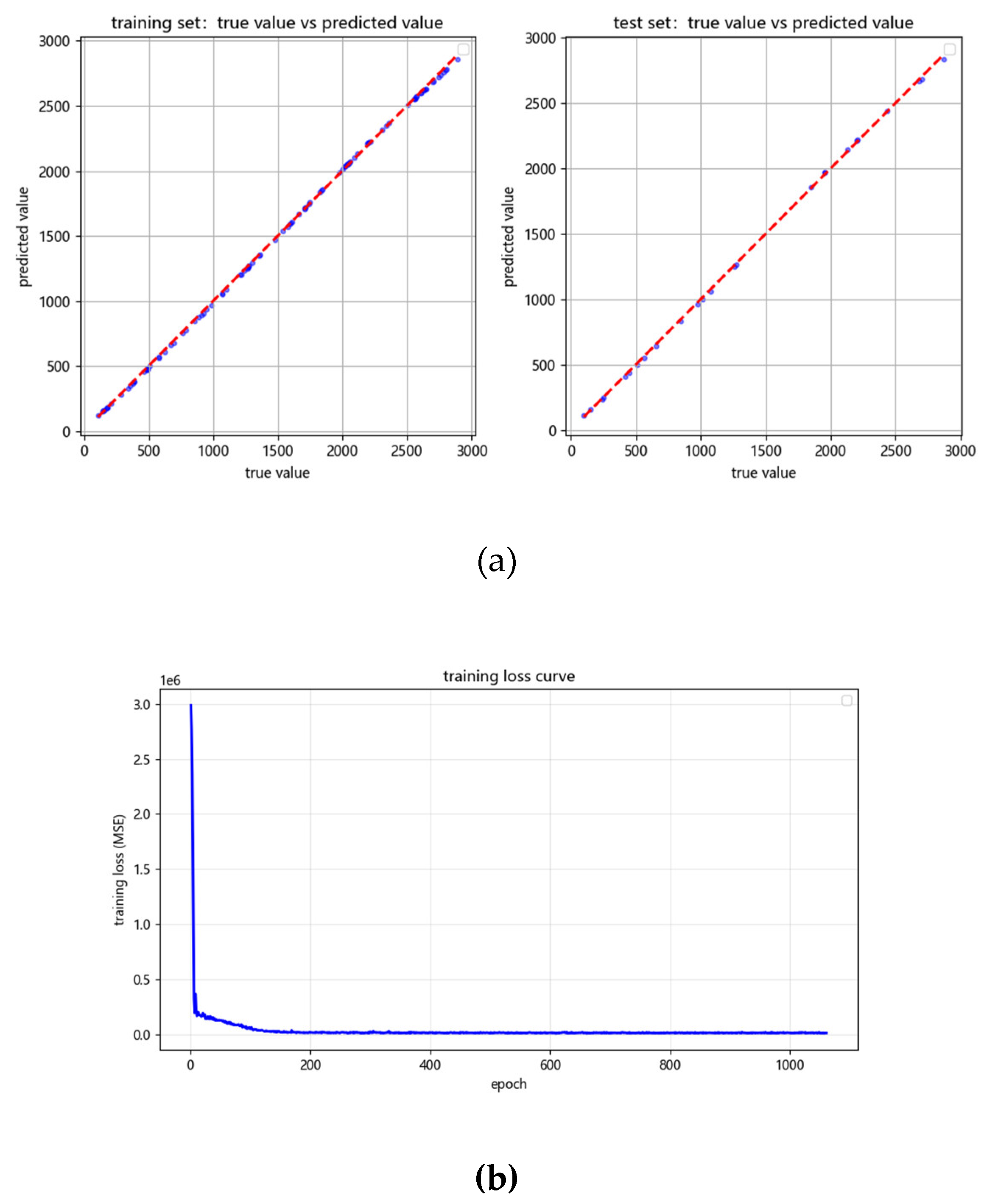
Figure 12.
Bar charts of R 2, RMSE, and MAE for each concentration interval.
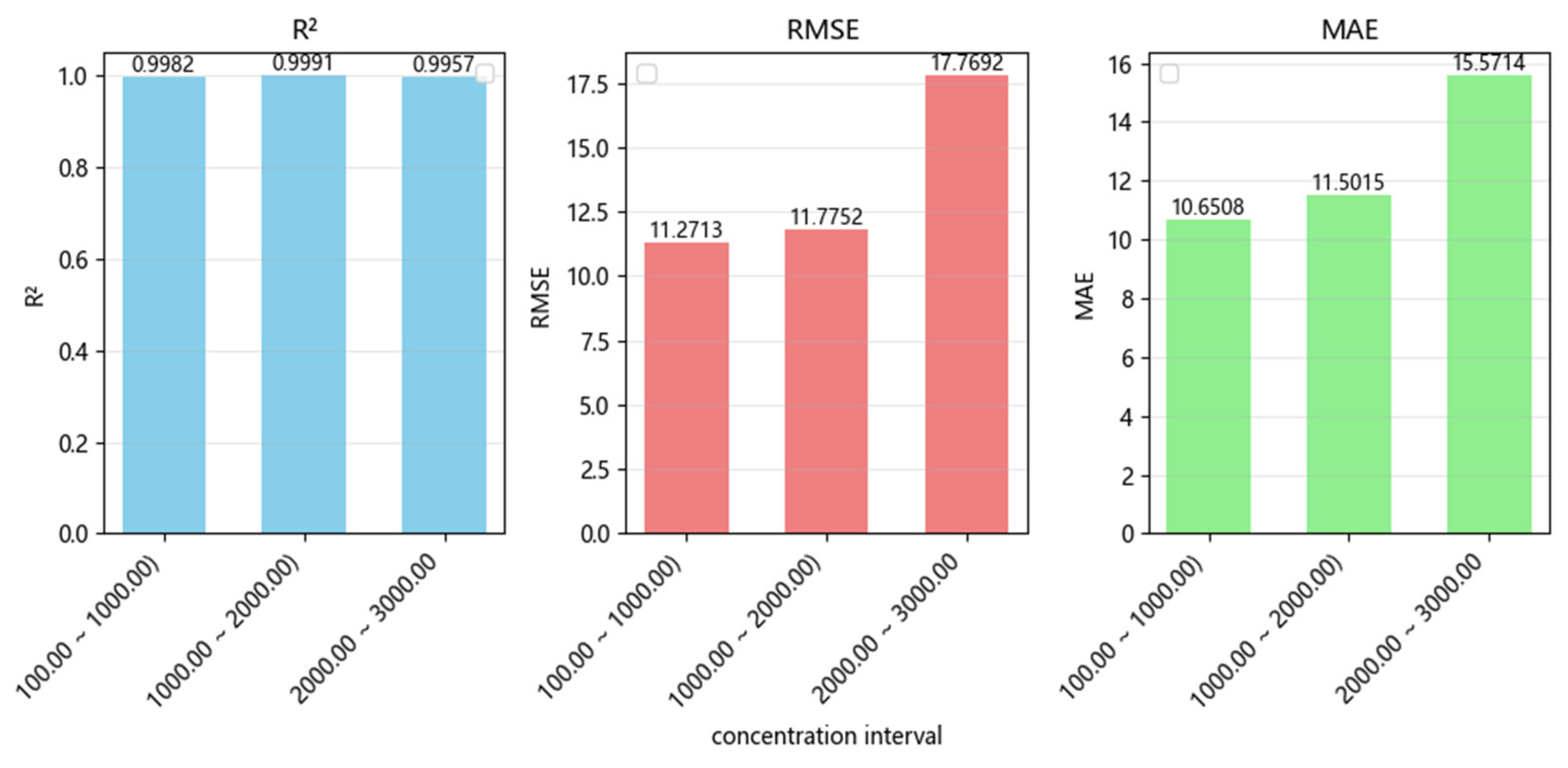
Figure 13.
Multi-dimensional visualization comparison of performance of various comparison models (a) Bar charts of R 2, RMSE, and MAE indicators for each model; (b) Comparison of model complexity and R 2 performance scatter plot; (c) Comparison chart of predicted and true values for each model’s training/testing set.
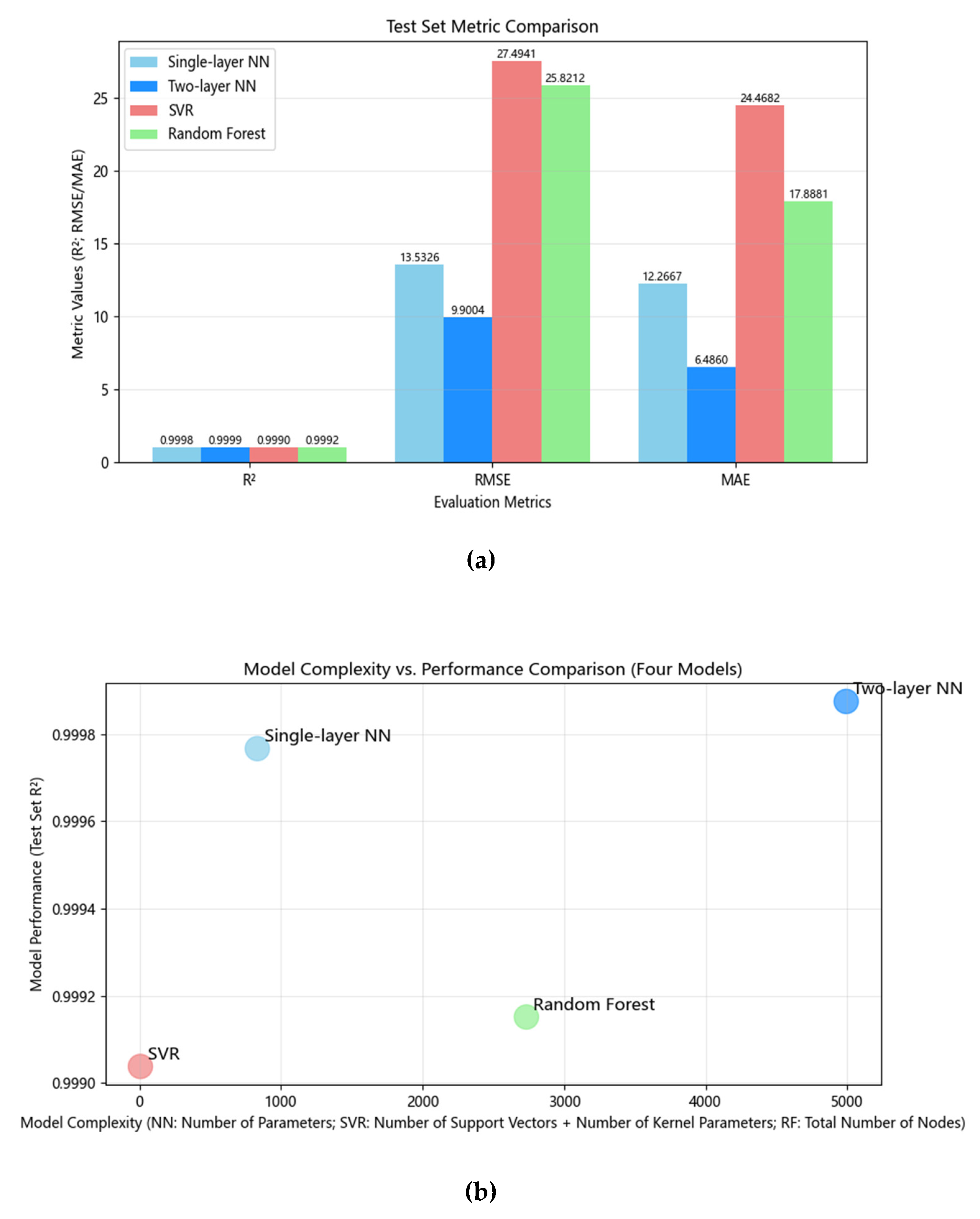
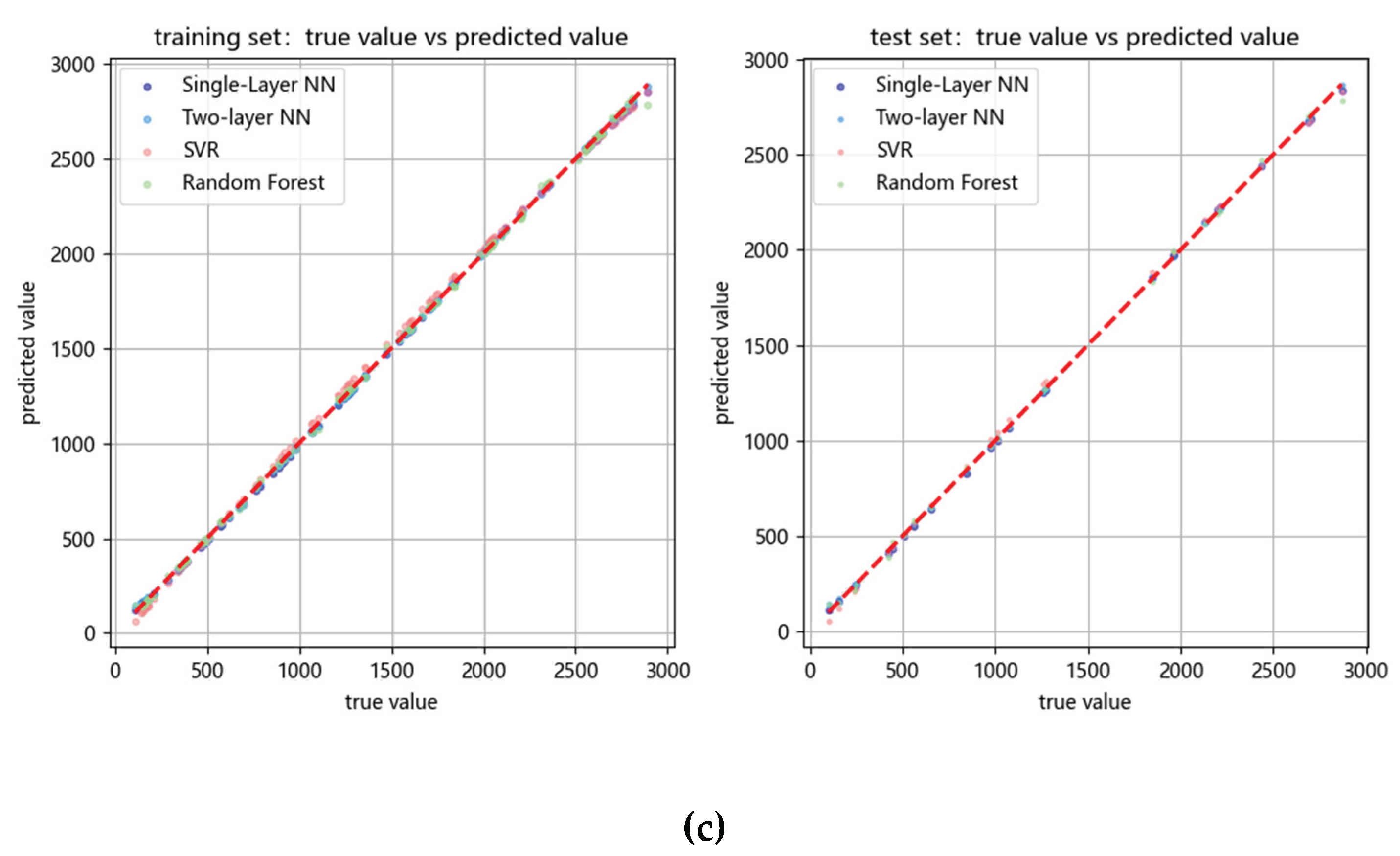

Table 1.
Overall performance metrics of the lightweight neural network model.
| Evaluation Metric | Training Set | Test Set |
|---|---|---|
| R2 | 0.9998 | 0.9998 |
| RMSE(ppm) | 12.0675 | 13.5326 |
| MAE(ppm) | 10.5598 | 12.2667 |
| Prediction Delay (s) | 0.8 | |
| Model Complexity (Parameters) | 833 (64 neurons in the hidden layer) |
Table 2.
Performance indicators for model concentration intervals.
| Concentration range (ppm) | R2 | RMSE(ppm) | MAE(ppm) |
|---|---|---|---|
| 100-1000 (low concentration) | 0.9983 | 11.2713 | 10.6508 |
| 1000-2000 (medium concentration) | 0.9990 | 11.7752 | 11.5015 |
| 2000-3000 (high concentration) | 0.9973 | 17.7692 | 15.5714 |
Table 3.
Performance indicators for model concentration intervals.
| Model Type | R2 | RMSE(ppm) | MAE(ppm) | Model complexity |
|---|---|---|---|---|
| Lightweight neural network | 0.9998 | 13.5326 | 12.2667 | 833 trainable parameters |
| SVR | 0.9990 | 27.4941 | 24.4682 | 4 support vectors |
| Random Forest Regression | 0.9992 | 25.8212 | 17.8881 | 2734 total nodes, integrated with 50 decision trees |
| FCNN-2 | 0.9999 | 9.9004 | 6.4860 | 4993 trainable parameters |
Disclaimer/Publisher’s Note: The statements, opinions and data contained in all publications are solely those of the individual author(s) and contributor(s) and not of MDPI and/or the editor(s). MDPI and/or the editor(s) disclaim responsibility for any injury to people or property resulting from any ideas, methods, instructions or products referred to in the content. |
© 2026 by the authors. Licensee MDPI, Basel, Switzerland. This article is an open access article distributed under the terms and conditions of the Creative Commons Attribution (CC BY) license (http://creativecommons.org/licenses/by/4.0/).
Copyright: This open access article is published under a Creative Commons CC BY 4.0 license, which permit the free download, distribution, and reuse, provided that the author and preprint are cited in any reuse.


