
Submitted:
01 February 2026
Posted:
05 February 2026
You are already at the latest version
Abstract
Accurate prediction of Electrocardiogram (ECG) signals is crucial for early diagnosis and continuous cardiac monitoring. To address the challenges posed by the non-stationary nature of ECG signals, this study introduces a novel deep learning prediction method that synergistically combines Variational Mode Decomposition (VMD), the Cao method, and a Long Short-Term Memory (LSTM) neural network. The proposed method first applies VMD to adaptively decompose the raw ECG signal into several Intrinsic Mode Functions (IMFs), which effectively reduces nonlinearity and non-stationarity. Subsequently, the Cao method is utilized to compute the minimum embedding dimension for each IMF, thereby optimally configuring the input structure for the LSTM network. Each IMF component is then predicted independently by an LSTM model trained with the Adam optimizer. The final reconstructed ECG signal is derived from the aggregate of these individual IMF predictions. Evaluated on the benchmark MIT-BIH Arrhythmia Database, the proposed method achieves a root mean square error (RMSE) of 0.001326 and a mean absolute error (MAE) of 0.001044, demonstrating high predictive precision. The results from a comparative study indicate that the proposed method surpasses several established prediction methods, confirming its effectiveness and potential for practical application in enhancing ECG signal analysis.
Keywords:
Cao method
; deep learning
; ECG
; LSTM neural network
; prediction
; VMD
1. Introduction
In recent years, with the increasing popularity of smart wearable devices, more and more people can now access real-time biometric signals conveniently and non-invasively. The wearable devices such as smartwatches, fitness trackers, and health monitors have democratized the monitoring of vital physiological parameters, enabling users to track key indicators like electrocardiogram (ECG), electroencephalogram (EEG), body temperature, and blood pressure. Among these indicators, ECG serves as a fundamental non-invasive tool for monitoring cardiac activity, playing a critical role in the early detection and diagnosis of cardiovascular diseases such as arrhythmias and myocardial infarctions.
Cardiovascular diseases, predominantly heart disease, remain the leading global cause of mortality, accounting for approximately 18 million annual deaths as per the World Health Organization's 2025 report. Accurate prediction of ECG signals is crucial for early detection of heart conditions like arrhythmia. This enables timely medical interventions, preventing disease progression and significantly reducing mortality rates.
With the development of deep learning technology, deep learning models are increasingly widely used for time series prediction. As a typical deep learning model, RNN (Recurrent Neural Network) has been applied in time series prediction [1,2,3,4]. Compared with the traditional time series prediction methods, RNN improves the prediction accuracy, but it still has the shortcomings of gradient disappearance and gradient explosion. LSTM is an improved RNN that overcomes the shortcomings of traditional RNN and is well suited for processing and predicting time-series data with time delays. Relevant literature shows that LSTM is indeed more effective than the traditional RNN model in the analysis and prediction of time series data [5,6]. At present, LSTM is widely used in natural language recognition [7,8,9], machine translation [10,11,12,13], and financial time series prediction [14,15,16]. In addition, LSTM has also been applied to time series prediction in other fields. In order to improve the accuracy of wind power forecasting, Sarkar et al. [17] proposed a novel deep learning model for wind power forecasting. The proposed prediction model combines an adaptive spectral block (ASB), an interactive convolution block (ICB), LSTM networks, and self-supervised learning (SSL). The experimental results show that the forecasting model improved the forecasting accuracy, with average reductions in MAE and RMSE of 5-8% and 8-12%, respectively. Jin et al. [18] used four popular Artificial Intelligence Neural Networks, namely CNN, RNN, LSTM and GRU, to predict random sea waves and conducted systematic comparative analysis. The results demonstrate that Compared with the other three kinds of artificial intelligence neural networks, LSTM shows good accuracy in short-term prediction, but it is more time-consuming. To enhance earthquake prediction precision, Kaushal et al. [19] predicted the earthquake by four deep learning models, namely RNN, LSTM, AdaBoost, and a hybrid RNN-LSTM model. Among these four models, the RNN-LSTM hybrid achieves an impressive accuracy rate of 98 %, significantly surpassing the other models. Khan et al. [20] proposed a traffic flow forecasting scheme based on the Tree-structured Parzen Estimator. The proposed scheme uses the Tree-structured Parzen Estimator to tune the hyperparameters of LSTM deep learning framework. Simulation results show that the proposed scheme exceeds the benchmark scheme in terms of prediction accuracy. To improve the precision of solar irradiance prediction, Liu et al. [21] proposed a VMD-FE-LSTM-Transformer forecasting model. The proposed model is optimized by Bayesian optimization and employs variational mode decomposition (VMD) and fuzzy entropy (FE) to decompose and reconstruct solar irradiance data. Compared with multiple forecasting models, the proposed model has the superior capability in single-step and multi-step forecasting.
This paper focuses on the prediction of ECG signals. Because an ECG signal is a nonlinear and non-stationary time series signal with an inherent random feature, it is difficult to predict accurately. To our knowledge, there are not many papers on predicting ECG signal at present, but there have been some papers that are explicitly related to ECG signal prediction [22,23,24,25]. In order to eliminate redundant data transmission within the body area network and reduce energy consumption, Wang et al. [26] proposed an ECG data fusion algorithm with synchronous prediction. The proposed algorithm is based on wavelet transform and LSSVM (least squares support vector machine). The experiment shows that the proposed algorithm significantly improves the accuracy of ECG prediction, with an RMSE of 0.0529. We proposed two ECG signal prediction methods, one based on ARIMA (Autoregressive Integrated Moving Average) model [27] and the other based on RBF (Radial Basis Function) neural network [28]. The prediction accuracy of the latter is higher than that of the former. To improve the accuracy of ECG signal forecasting, Ratna Prakarsha et al. [29] proposed an artificial neural network method for predicting ECG signals and compared it with a conventional method of using LMS (Least Mean Square) filter. The experiment proves the superiority of the method of artificial neural network over the method of LMS filter. Dudukcu et al. [30] proposed a hybrid deep neural network model for chaotic time series prediction. The proposed model is formed by combining different neural network layers, the temporal convolutional neural network (TCN) with RNN. The simulation results show that the proposed model has an average MAE of 0.0051 and an average RMSE of 0.0082 on ECG arrhythmia dataset. In the study carried out by Zacarias et al. [31], a model based on LSTM neural network with two hidden layers was proposed for ECG signal forecasting. The results show that the average RMSE of the proposed forecasting model is 0.0070±0.0028, and the average MAE is 0.0522±0.0098.
Due to the generally low prediction accuracy of ECG signal prediction methods mentioned above, we propose a novel deep learning prediction method for ECG signals using VMD, Cao method, and a LSTM neural network. The rest of this paper is organized as follows: Section 2 presents the materials and methods used to address ECG prediction. Section 3 presents a discussion of the results; Section 4 concludes the paper.
2. Materials and Methods
2.1.VMD
Variational mode decomposition (VMD) decomposes an input signal into a series of discrete band-limited intrinsic mode functions (IMFs) around the center frequency. In time series prediction, the function of VMD is to reduce the non-stationary character of time series, which is helpful to improve the accuracy of prediction. Each IMF component is obtained through the following three steps:
Step 1: Calculate the analytic signal of each modal function by Hilbert transform
Step 2: Multiply the analytical signal by the estimated center frequency , and move it to the base frequency spectrum, which is
Step 3: Estimate the bandwidth of each mode by Gaussian smoothing of the demodulated signal, i.e., the L2 norm of the gradient. The constrained variational model is
where x is the input signal and is the Euclidian distance. In order to find the optimal solution of the above problem, turn the constrained variational model into an unconstrained variational model by introducing the quadratic penalty factor and Lagrange multiplication operator . The extended Lagrange expression is
Find the saddle point of the extended Lagrange expression using the alternating direction multiplier method (ADMM) [32] to solve the extended Lagrange problem. The saddle point is obtained by alternating renewal . The specific implementation process of VMD is as follows:
Step 1: Initialize , and set n = 0.
Step 2: Update , and . The formulas for this are
Where , and are the Fourier transforms of the signals , , and , respectively. β is the step update coefficient.
Step 3: Repeat step 2 until the convergence condition is reached
where ε is a judgment threshold.
Before VMD, the number K of IMFs needs to be predetermined. K can be determined according to the ratio Rres of residual energy to the original signal energy. Rres is defined as follows:
where X(n) is the original signal, uk (n) is the IMF, and N is the sample number. When Rres is less than 1% and there is no significant downward trend, the number K can be determined [33]. For the No. 100 ECG data, the Rres of VMD with different K are shown in Table 1.
Table 1 shows that the Rres has no obvious downward trend when K =14. Therefore, we set K =14 in the experiment.
The No. 100 ECG was decomposed into 14 IMFs by VMD as shown in Figure 1. IMF1 is the residual, and IMF2-IMF14 is the component, sorted from low to high frequency.
2.2. Cao Method
Cao method was proposed to determine the minimum embedding dimension of a time series by Cao [34]. In Cao method, the time-delay parameter τ is necessary before the minimum embedding dimension is determined. For a time series ,the time-delay vectors can be reconstructed as follows:
Cao method is described as follows:
where m is the embedding dimension, τ is the time delay, is the ith reconstructed vector with embedding dimension m, is Euclidian distance, is an integer which is the nearest neighbor of . If stops changing when m is greater than the value m0, m0+1 is the minimum embedding dimension.
The embedding dimension m of IMF5 is determined by Cao method, as shown in Figure 2.
According to Figure 2, we obtain the embedding dimension m = 7 of IMF5. In the experiment, we set τ = 1 and obtain the minimum embedding dimensions m of each IMF, as shown in Table 2.
The minimum embedding dimension m is the input dimension of LSTM neural network.
2.3. LSTM Neural Network
In 1997, Hochreiter and Schmidhuber proposed LSTM based on RNN neural network [35]. As an improved RNN model, LSTM solves the problems of gradient disappearance and gradient explosion that RNN cannot overcome. With the rapid development and popularization of deep learning, LSTM is widely used in time series applications.
Each LSTM unit is composed of a memory cell and three gates: an input gate, a forget gate, and an output gate. The functions of these three gates are: the input gate decides the information that should be input; the forget gate determines the information that should be discarded; the output gate decides the information that should be output. The architecture of LSTM unit is shown in Figure 3.
The forget gate is expressed in the following formula:
The input gate is expressed in the following formulas:
The output gate is expressed in the following formulas:
where and denotes weight matrices and bias vectors of gates, respectively. In addition, and tanh are the activation functions between different layers, is the current state of the cell, is the unit state of the current input, and is the current output of the cell. The expressions of and tanh are as follows:
By introducing cell state and three gate structures of forgetting gate, input gate and output gate, LSTM has the ability of long-term and short-term memory, thus solving the problems of gradient disappearance and gradient explosion of RNN. Compared with other neural networks, LSTM is more suitable for time series data prediction.
2.4. Sliding window approach
ECG prediction is a predictive modeling technique that utilizes historical ECG data to make projections about future occurrences. A typical network structure of LSTM for ECG prediction is shown in Figure 4.
In Figure 4, is the predicted value of . In order to obtain , time series data are required as inputs to the LSTM input layer. A sliding window approach is used to solve the input size of LSTM prediction model [29,31]. For example, when the sliding window size is 5, the sliding window method is used to predict sequences as shown in Table 3.
The size m of the sliding window affects the accuracy of prediction. Different m results in different prediction accuracies. In this paper, Cao method is used to determine the optimal sliding window size m. The optimal sliding window size m is the input size of LSTM input layer.
2.5. Proposed Method
Based on the study of ECG signal prediction, this paper proposes a deep learning prediction method of ECG signal. Its flowchart is shown in Figure 5.
The prediction steps of the proposed method are as follows:
Step 1: Denoising processing before ECG prediction is necessary. In this paper, as the ECG data from the MIT-BIH Arrhythmia Database have been denoised, there is no need for denoising processing.
Step 2: Decompose an ECG signal into K IMFs by VMD. In the experiment, we use K = 14 to get a better prediction result.
Step 3: Determine the embedding dimension by Cao method. The embedding dimension is the input size of the LSTM neural network.
Step 4: Establish a LSTM neural network according to the trained set and use it to predict the test set of each IMF.
Step 5: Add the prediction results of all LSTM neural networks to obtain the final ECG signal prediction result.
Step 6: Analyze the prediction error and compare it to other prediction methods.
3. Results and Discussion
The common performance measures of prediction methods are root mean square error (RMSE), mean absolute error (MAE), mean absolute percentage error (MAPE), and R-square (R2), defined as
where is the predicted value of , is the length of , and is the mean of .
All ECG data in the simulation experiment are from the MIT-BIH Arrhythmia Database [36]. We selected the No.100 ECG signal, which consists of 2,768 data points, for the experiment. We used two-thirds of the No.100 ECG signal as the training set (i.e. 1845 data points) and the remaining one-third as the test set (i.e. 923 data points). The original No. 100 ECG signal is shown in Figure 6.
All experiments were carried out in MATLAB and Python compiling environment. The LSTM model was implemented in a Theano framework based on Keras deep learning tools. The value of the parameter epochs in LSTM neural network has a significant impact on the prediction results. The impact of different values of the parameter epoch on prediction accuracy in the case of LSTM parameter batch_size=4 is shown in Table 4.
Table 4 shows that with the LSTM neural network parameter batch_size=4, good prediction performance is achieved with the LSTM neural network parameter epochs=250, where RMSE=0.001326 and MAE=0.001044.
In the experiment, the values of each parameter in LSTM are epochs=250, batch_size=4, optimizer=Adam, loss=mean_squared_error, activa-tion=Relu. The prediction method proposed in this paper was used to predict the test set of 923 ECG data, as shown in Figure 7.
In Figure 7, raw signal represents the original ECG signal and test prediction represents the predicted ECG signal of the test set. Figure 7 shows that the predicted ECG waveform overlaps almost perfectly with the original ECG waveform. In order to observe the degree of fit between the original ECG signal waveform and the predicted ECG signal waveform, local amplification is shown in Figure 8.
In Figure 8, The local magnification range is [165,185]. Figure 8 shows that even after amplification, the predicted ECG signal waveform still overlaps well with the original ECG signal waveform. The prediction indexes of the test set are shown in Table 5.
Table 5 shows that the RMSE, MAE, and MAPE are very small and R2 is close to 1. This indicates that the prediction method proposed in this paper has high prediction accuracy.
To evaluate the performance of the prediction method, the proposed method in this paper was compared with the prediction methods in the existing literature [23,24,25,27,28,30,31] on the same dataset (the No.100 ECG data). The comparison results are shown in Table 6.
In Table 6, The values of 0.0470 and 0.0070 in Zacarias et al. [31] are approximate values read from the bar chart in Zacarias et al. [31].The bar charts of MAE and RMSE in Table 6 are shown in Figure 9 and Figure 10, respectively.
Figure 9 and Figure 10 visually demonstrate that the MAE and RMSE of this paper are significantly smaller than those of the existing literature [23,24,25,27,28,30,31]. This illustrates that the prediction accuracy of the prediction method proposed in this paper is higher than that of the prediction methods in the existing literature [23,24,25,27,28,30,31].
In addition, the prediction method proposed in this paper was compared with several popular hybrid prediction methods, such as the method based on WT, PSR, and RBF neural network (WT-PSR-RBF for short); the method based on empirical mode decomposition (EMD), PSR, and RBF neural network (EMD-PSR-RBF for short); the method based on VMD, PSR, and BP neural network (VMD-PSR-BP for short); and the method based on VMD, generalized regression neural network (GRNN) , and PSR (VMD-PSR-GRNN for short). The experimental data are the No. 100 ECG data. The trained set has 1845 data points and the test set has 923 data points. The experimental results are shown in Table 7.
It is obvious from Table 7 that the prediction performance of this paper is superior to that of WT-PSR-RBF, EMD-PSR-RBF, VMD-PSR-BP and VMD-PSR-GRNN.
We also compared the prediction method proposed in this paper with single deep learning prediction methods. The comparison results are shown in Table 8 and Figure 11.
Table 8 shows that the RMSE and MAE of this paper are obvious smaller than those of LSTM, MLP and CNN.
4. Conclusions
In order to improve the prediction accuracy of ECG signals, a deep learning hybrid prediction method based on VMD, Cao method, and a LSTM neural network is proposed in this paper. The prediction performance of the prediction method proposed in this paper is evaluated by using the No.100 ECG signal from the MIT-BIH arrhythmia database as the data source. The experimental results show that the prediction performance of the prediction method proposed in this paper not only exceeds the prediction performance of the existing literature [23,24,25,27,28,30,31], but also surpasses the prediction performance of several popular hybrid prediction methods, as well as single deep learning prediction methods. We draw a conclusion that the prediction method proposed in this paper significantly improves the prediction accuracy of ECG signals.
Future work will focus on two directions: (1) Applying optimization algorithms to optimize the hyperparameters of LSTM, further improving the prediction accuracy of ECG signals; (2) Expanding muti-step prediction of ECG signals. Compared with one-step prediction of ECG signals, multi-step prediction of ECG signals can provide longer warning windows and enhance proactive intervention capabilities.
Author Contributions
Conceptualization, T.Q. and F.H.; methodology, F.H.; software, L.W. and F.H.; validation, G.O., X.Z. and F.H.; formal analysis, X.Z.; investigation, D.W.; resources, T.Q.; data curation, F.H.; writing—original draft preparation, F.H.; writing—review and editing, L.W.; visualization, X.Z.; supervision, G.O. and D.W.; project administration, X.Z.; funding acquisition, T.Q. All authors have read and agreed to the published version of the manuscript.
Funding
This research was supported partially by the Guangxi Key Research and Development Program (No.2025FN9701139&2025FN9622746), in part by the Guangxi Science and Technology Base and Talent Special Project (No. AD25069071).
Institutional Review Board Statement
Not applicable.
Informed Consent Statement
Not applicable.
Data Availability Statement
In this study, ECG data are from the MIT-BIH Arrhythmia Database. Available online: https://www.physionet.org/content/mitdb/1.0.0/
Conflicts of Interest
The authors declare no conflicts of interest.
References
- Marsetič, A.; Kanjir, U. Forecasting Vegetation Behavior Based on PlanetScope Time Series Data Using RNN-Based Models. IEEE Journal of Selected Topics in Applied Earth Observations and Remote Sensing 2024, 17, 5015–5025. [Google Scholar] [CrossRef]
- Li, L.; Yan, J.; Zhang, Y.; Zhang, J.; Bao, J.; Jin, Y.; Yang, X. Learning Generative RNN-ODE for Collaborative Time-Series and Event Sequence Forecasting. IEEE Transactions on Knowledge and Data Engineering 2023, 35, 7118–7137. [Google Scholar] [CrossRef]
- Hwan Seo, J.; Kim, K. -D. An RNN-Based Adaptive Hybrid Time Series Forecasting Model for Driving Data Prediction. IEEE Access 2025, 13, 54177–54191. [Google Scholar] [CrossRef]
- Cai, C.; Zhang, L.; Zhou, J. DMPR: A novel wind speed forecasting model based on optimized decomposition, multi-objective feature selection, and patch-based RNN. Energy 2024, 310, 133277. [Google Scholar] [CrossRef]
- Palangi, H.; Ward, R.; Deng, L. Distributed Compressive Sensing: A Deep Learning Approach. IEEE Transactions on Signal Processing 2016, 64(17), 4504–4518. [Google Scholar] [CrossRef]
- Palangi, H.; Deng, L.; Shen, Y.; Gao, J.; He, X.; Chen, J.; Song, X.; Ward, R. Deep Sentence Embedding Using Long Short-Term Memory Networks: Analysis and Application to Information Retrieval. IEEE-ACM Trans Audio Speech Lang 2016, 24(4), 694–707. [Google Scholar] [CrossRef]
- Han, Y.; Han, Y.; Jiang, Q. A Study on the STGCN-LSTM Sign Language Recognition Model Based on Phonological Features of Sign Language. IEEE Access 2025, 13, 74811–74820. [Google Scholar] [CrossRef]
- Jorge, J.; Giménez, A.; Silvestre-Cerdà, J. A.; Civera, J.; Sanchis, A.; Juan, A. Live Streaming Speech Recognition Using Deep Bidirectional LSTM Acoustic Models and Interpolated Language Models. IEEE/ACM Transactions on Audio, Speech, and Language Processing 2022, 30, 148–161. [Google Scholar] [CrossRef]
- Kusumawardani, R. P.; Kusumawati, K. N. Named entity recognition in the medical domain for Indonesian language health consultation services using bidirectional-lstm-crf algorithm. Procedia Computer Science 2024, 245, 1146–1156. [Google Scholar] [CrossRef]
- Xiao, Q.; Chang, X.; Zhang, X.; Liu, X. Multi-Information Spatial–Temporal LSTM Fusion Continuous Sign Language Neural Machine Translation. IEEE Access 2020, 8, 216718–216728. [Google Scholar] [CrossRef]
- Limenih, H. H.; Adege, A. B.; Alene, A. Y.; Demasu, H. T.; Belachew, H. M. Automatic Identification of Amharic Text Idiomatic Expressions Using a Deep Learning Approach. IEEE Access 2025, 13, 83095–83106. [Google Scholar] [CrossRef]
- Zhang, Z.; Chen, Y.; Zhang, J. Neural Machine Translation in Electrical Engineering With Cross-Layer Information Fusion and Multiple Positional Mapping. IEEE Access 2025, 13, 135359–135372. [Google Scholar] [CrossRef]
- Su, C.; Huang, H.; Shi, S.; Jian, P.; Shi, X. Neural machine translation with Gumbel Tree-LSTM based encoder. Journal of Visual Communication and Image Representation 2020, 71, 102811. [Google Scholar] [CrossRef]
- Gajamannage, K.; Park, Y.; Jayathilake, D. I. Real-time forecasting of time series in financial markets using sequentially trained dual-LSTMs. Expert Systems with Applications 2023, 223, 119879. [Google Scholar] [CrossRef]
- Saâdaoui, F.; Rabbouch, H. Financial forecasting improvement with LSTM-ARFIMA hybrid models and non-Gaussian distributions. Technological Forecasting and Social Change 2024, 206, 123539. [Google Scholar] [CrossRef]
- Almusfar, L. A.; Mallouli, F. Deep Learning-Based Financial Forecasting with Post-Quantum Cryptographic Integration: A CNN-LSTM and F2N-ECC Hybrid Framework. Procedia Computer Science 2025, 270, 4573–4584. [Google Scholar] [CrossRef]
- Sarkar, M. R.; Anavatti, S. G.; Ferdaus, M. M.; Dam, T. ASPEN-WIND: Adaptive spectral and self-supervised interactive CNN-LSTM for enhanced wind power forecasting. Expert Systems with Applications 2026, 296, 129171. [Google Scholar] [CrossRef]
- Jin, X.; Dai, C.; Tao, Y.; Zhang, F. A comparative study of RNN, CNN, LSTM and GRU for random sea wave forecasting. Ocean Engineering 2025, 338, 122013. [Google Scholar] [CrossRef]
- Kaushal, A.; Gupta, A. K.; Sehgal, V. K. Earthquake prediction optimization using deep learning hybrid RNN-LSTM model for seismicity analysis. Soil Dynamics and Earthquake Engineering 2025, 195, 109432. [Google Scholar] [CrossRef]
- Khan, H. M.; Khan, A.; Villar, S. G.; Lopez, L. A. D.; Almaleh, A.; Al-Qahtani, A. M. A Comparative Study of Optimized-LSTM Models Using Tree-Structured Parzen Estimator for Traffic Flow Forecasting in Intelligent Transportation. Computers, Materials and Continua 2025, 83, 3369–3388. [Google Scholar] [CrossRef]
- Liu, Z.; Zhao, X. LSTM-Transformer with decomposition–reconstruction for enhanced solar irradiance forecasting incorporating meteorological variables. Renewable Energy 2026, 258, 124971. [Google Scholar] [CrossRef]
- Wei, C. X.; Zhang, C.; Wu, M. A study on the universal method of EEG and ECG prediction. Proceedings of 2017 10th International Congress on Image and Signal Processing, BioMedical Engineering and Informatics (CISP-BMEI), Shanghai, China; 2017, pp. 1–5.
- Sun, Z. -G.; Lei, Y.; Wang, J.; Liu, Q.; Tan, Q.-Q. An ECG signal analysis and prediction method combined with VMD and neural network. Proceedings of 2017 7th IEEE International Conference on Electronics Information and Emergency Communication (ICEIEC), Macau; 2017, pp. 199–202.
- Sun, Z. G.; Wang, Q.L.; Xue, Q.D.; Liu, Q.; Tan, Q.Q. Data Prediction of ECG Based on Phase Space Reconstruction and Neural Network. Proceedings of 2018 8th International Conference on Electronics Information and Emergency Communication (ICEIEC), Beijing, China; 2018, pp. 162–165.
- Su, F.; Dong, H. S. Prediction of ECG Signal Based on TS Fuzzy Model of Phase Space Reconstruction. Proceedings of 2019 12th International Congress on Image and Signal Processing, BioMedical Engineering and Informatics (CISP-BMEI), Suzhou, China; 2019, pp. 1–6.
- Wang, R.-Y.; Zhai, M.-L.; Wu, D.-P. Time series data aggregation algorithm with synchronous prediction for WBAN. Journal on Communications 2015, 36, 13–21. [Google Scholar]
- Huang, F.Y.; Qin, T. F.; Wang, L. M.; Wan, H. B.; Ren, J. Y. An ECG Signal Prediction Method Based on ARIMA Model and DWT. Proceedings of IEEE 4th Advanced Information Technology, Electronic and Automation Control Conference (IAEAC), Chengdu, China, 2019; pp. 1298–1304. [Google Scholar]
- Huang, F.; Qin, T.; Wang, L.; Wan, H. Hybrid Prediction Method for ECG Signals Based on VMD, PSR, and RBF Neural Network. BIOMED RESEARCH INTERNATIONAL 2021, 2021, 6624298. [Google Scholar] [CrossRef]
- Ratna Prakarsha, K.; Sharma, G. Time series signal forecasting using artificial neural networks: An application on ECG signal. Biomedical Signal Processing and Control 2022, 76, 103705. [Google Scholar] [CrossRef]
- Dudukcu, H. V.; Taskiran, M.; Cam Taskiran, Z. G.; Yildirim, T. Temporal Convolutional Networks with RNN approach for chaotic time series prediction. Applied Soft Computing 2023, 133, 109945. [Google Scholar] [CrossRef]
- Zacarias, H.; Marques, J. A. L.; Felizardo, V.; Pourvahab, M.; Garcia, N. M. ECG forecasting system based on long short-term memory. Bioengineering 2024, 11, 89. [Google Scholar] [CrossRef]
- Tosserams, S.; Etman, L. F. P.; Papalambros, P. Y. An augmented Lagrangian relaxation for analytical target cascading using the alternating direction method of multipliers. Structural and Multidisciplinary Optimization 2006, 31(3), 176–189. [Google Scholar] [CrossRef]
- Liu, Y. S.; Yang, C. H.; Keke; Gui, W.H. Non-ferrous metals price forecasting based on variational mode decomposition and LSTM network. Knowledge-Based Systems 2019, 188, 105006. [Google Scholar] [CrossRef]
- Cao, L. Practical method for determining the minimum embedding dimension of a scalar time series. Physica D Nonlinear Phenomena 1997, 110(1-2), 43–50. [Google Scholar] [CrossRef]
- Hochreiter, S.; Schmidhuber, J. Long Short-Term Memory. Neural Computation 1997, 9(8), 1735–1780. [Google Scholar] [CrossRef] [PubMed]
- MIT-BIH Arrhythmia Database. Available online: https://www.physionet.org/content/mitdb/1.0.0/.
Figure 1.
The decomposition by VMD. (a) IMF1-IMF7; (b) IMF8-IMF14.
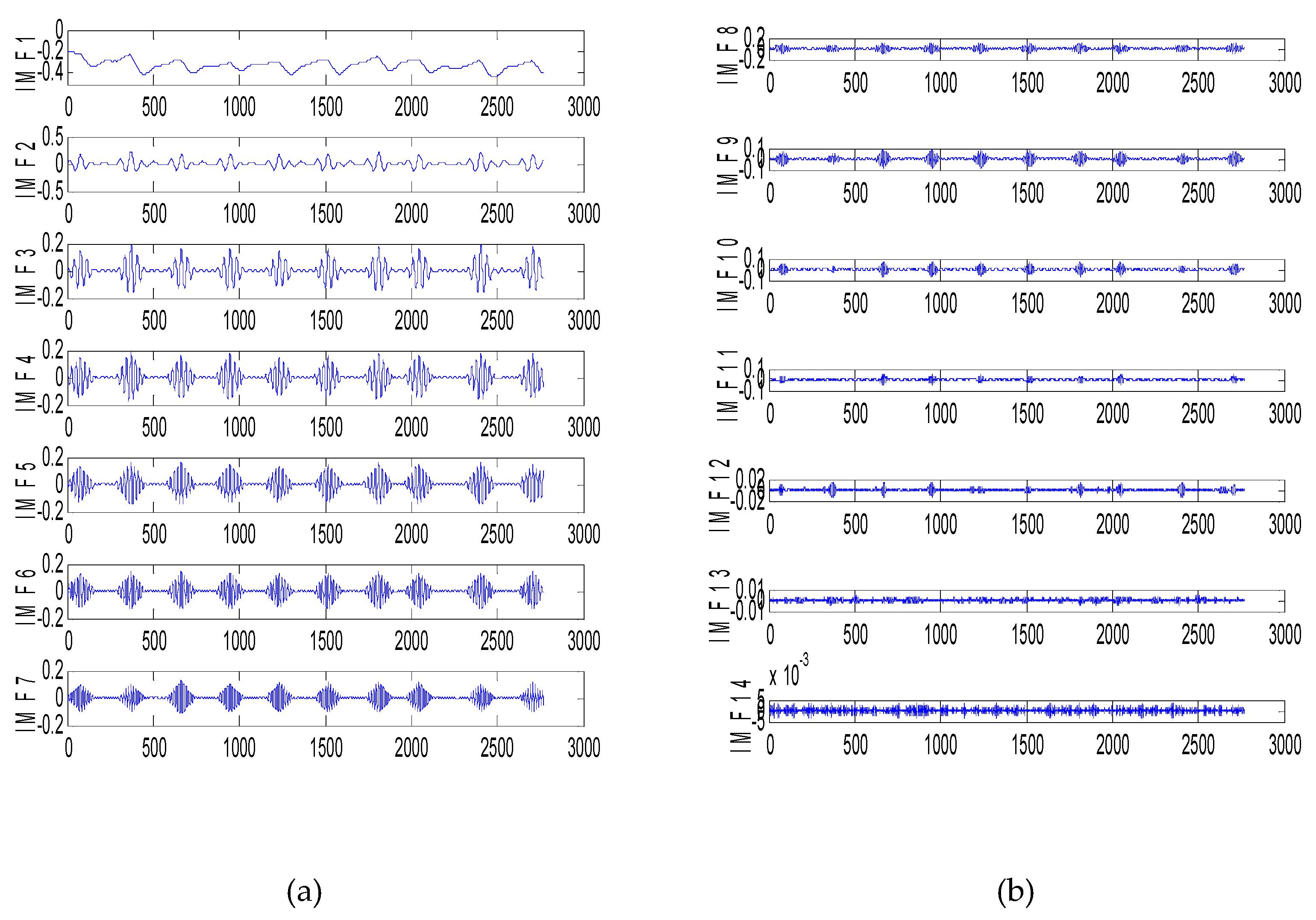
Figure 2.
The determination of m by Cao method.
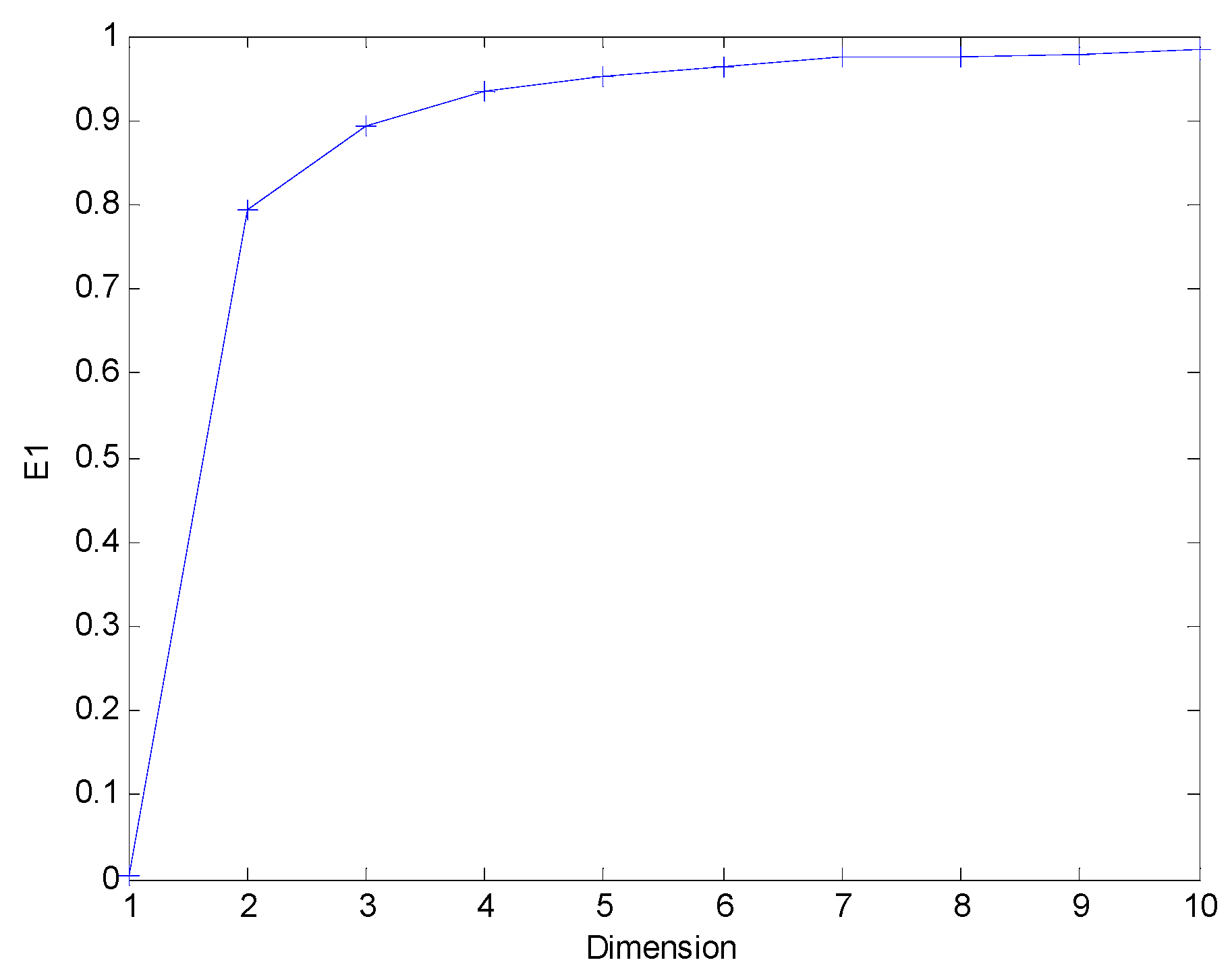
Figure 3.
The architecture of LSTM unit.
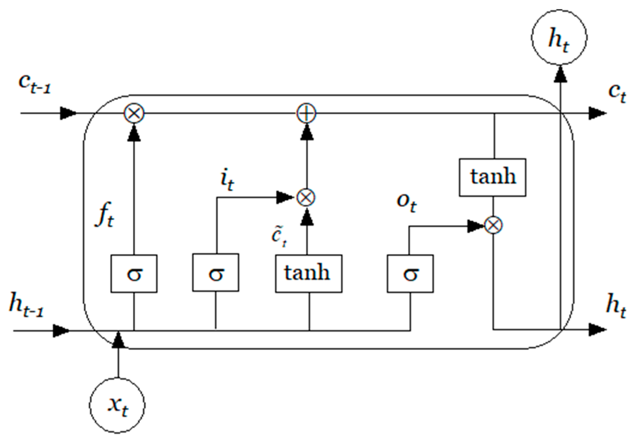
Figure 4.
Network structure of LSTM prediction model.
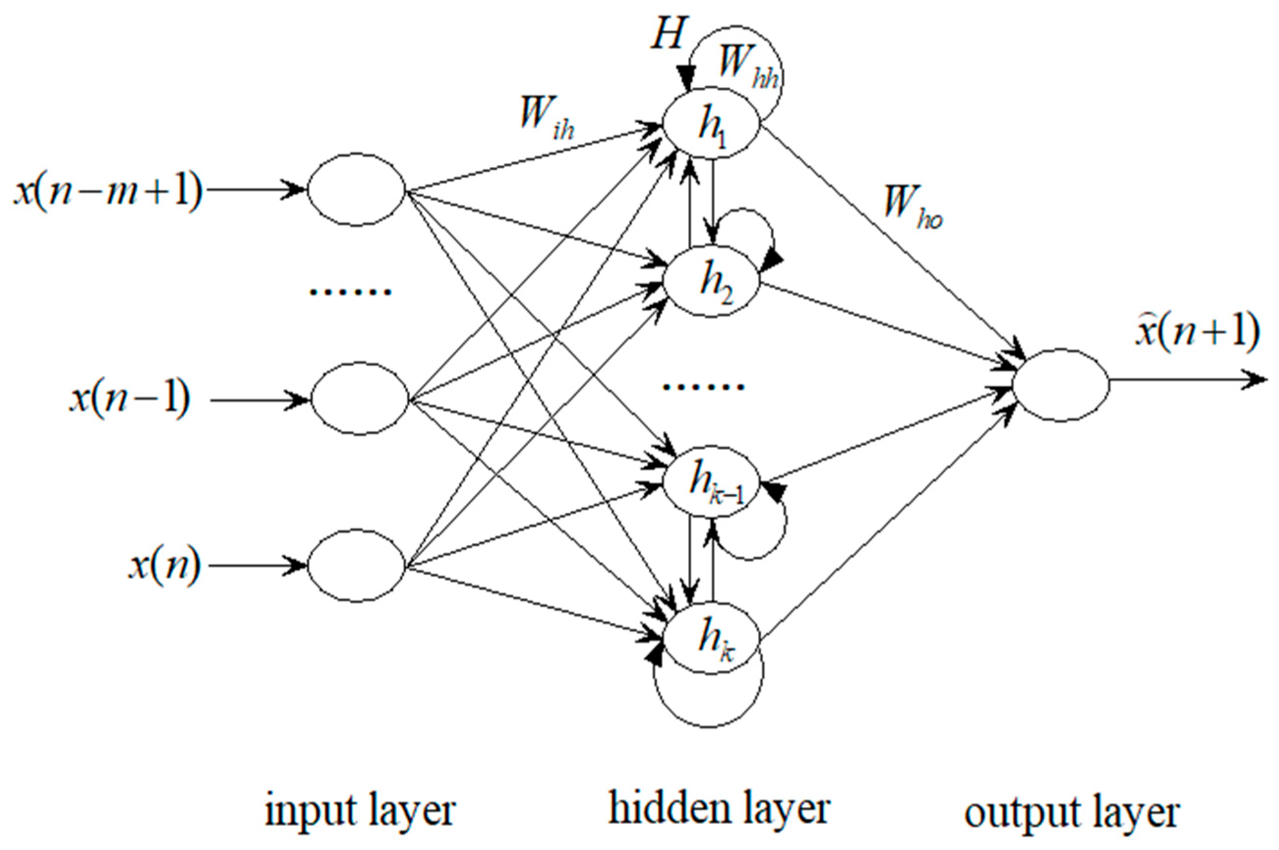
Figure 5.
Flowchart of the proposed method.
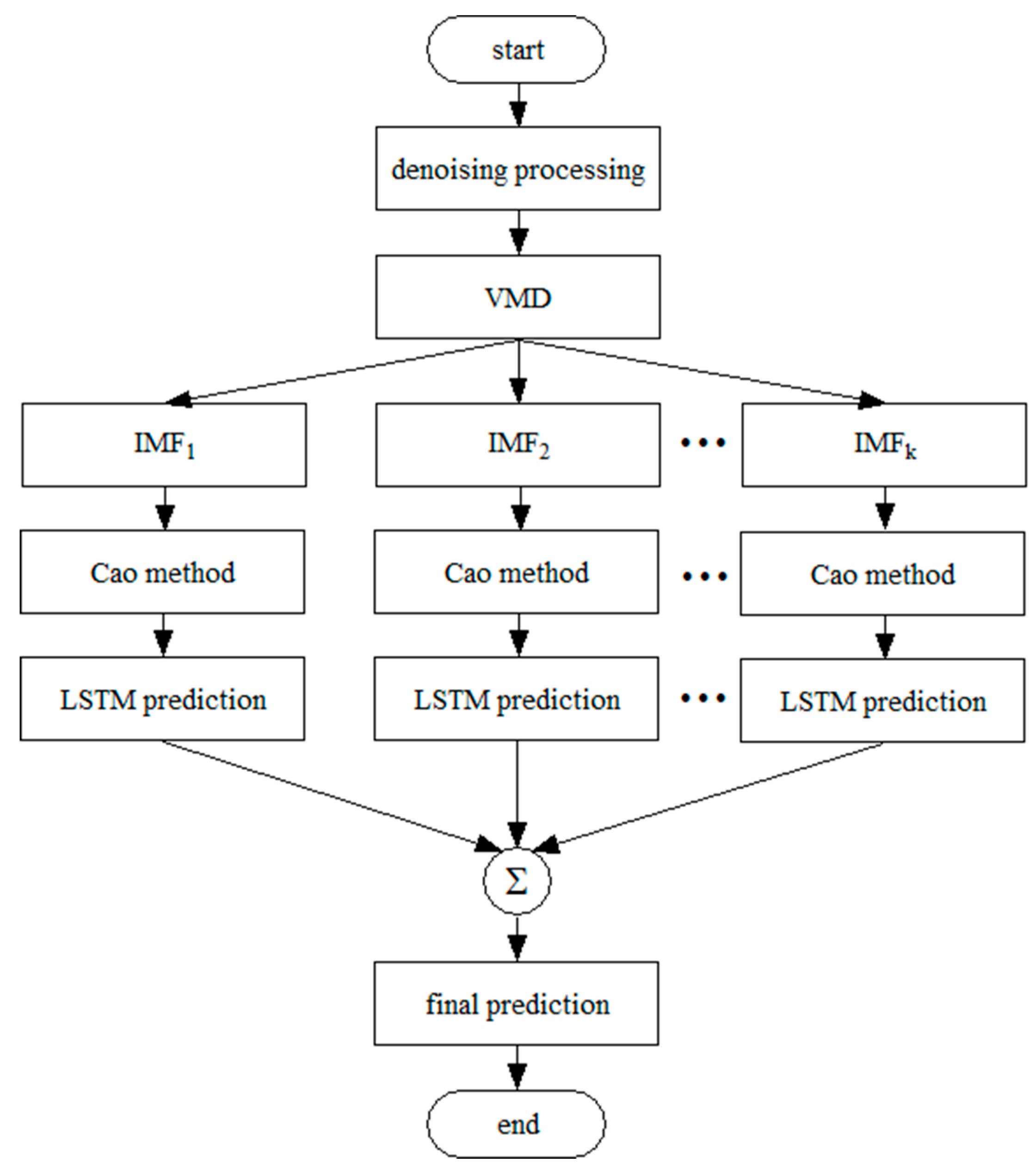
Figure 6.
The No.100 ECG signal.
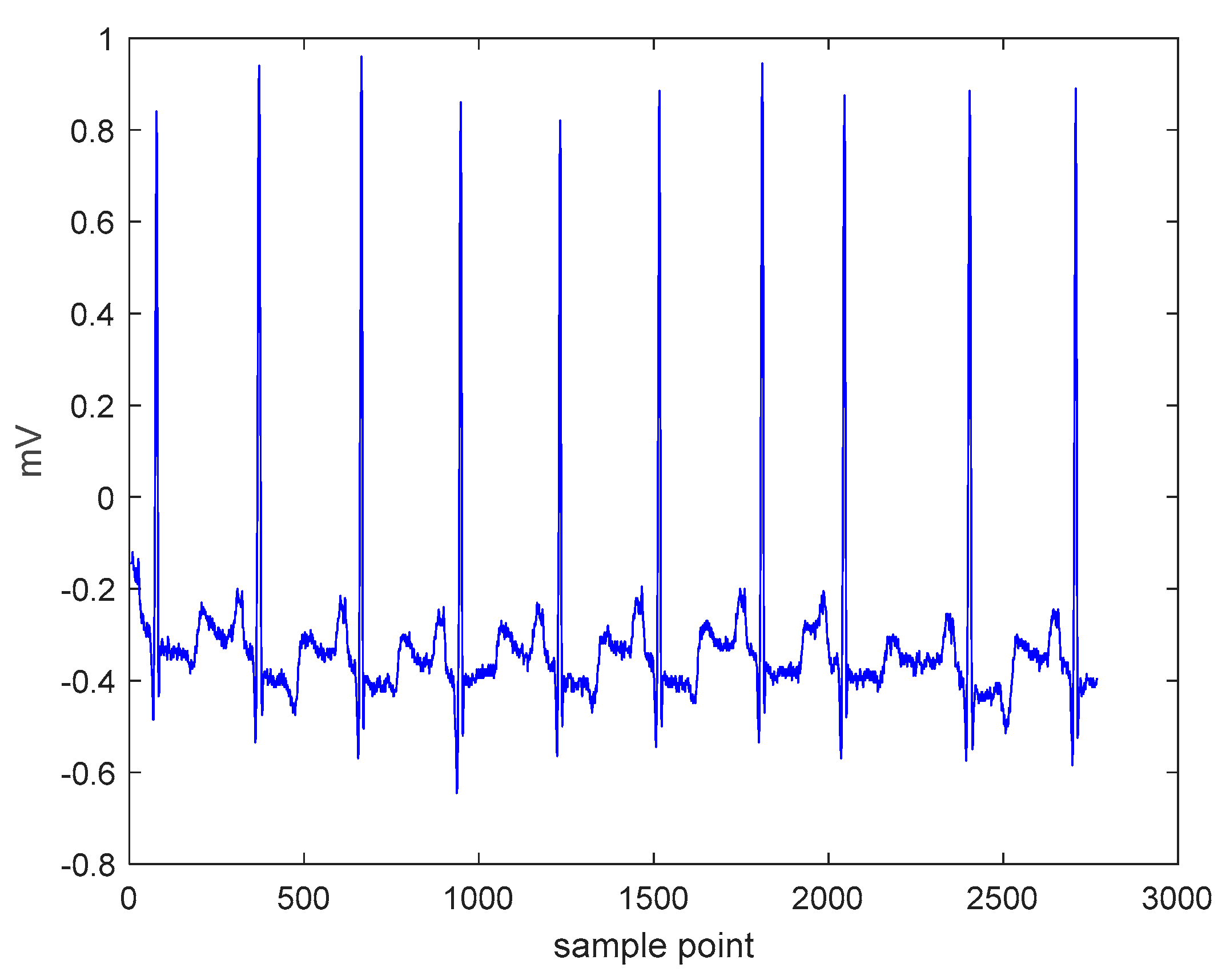
Figure 7.
The prediction waveform of the test set.
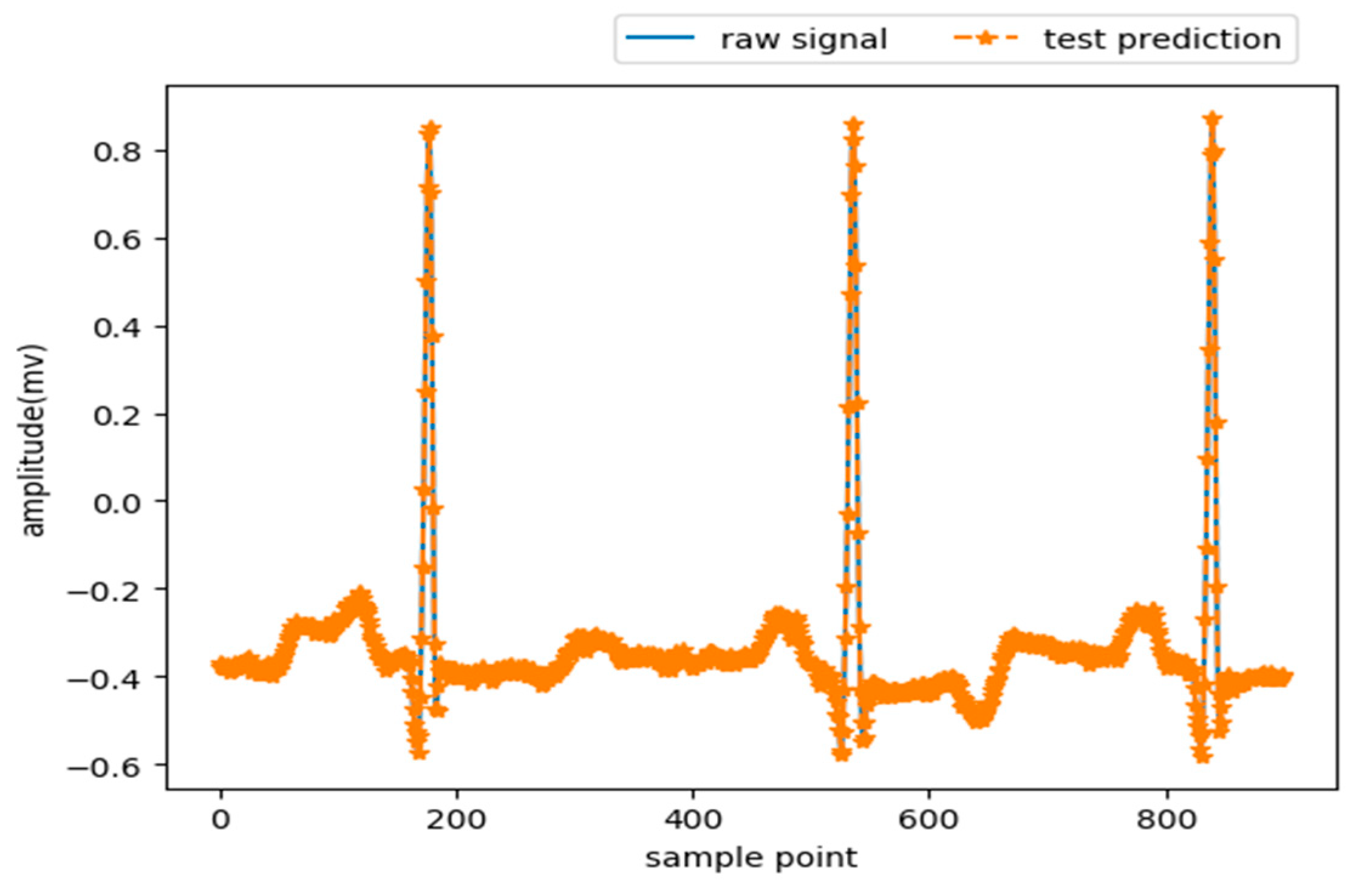
Figure 8.
The local amplification of the ECG signal waveform.
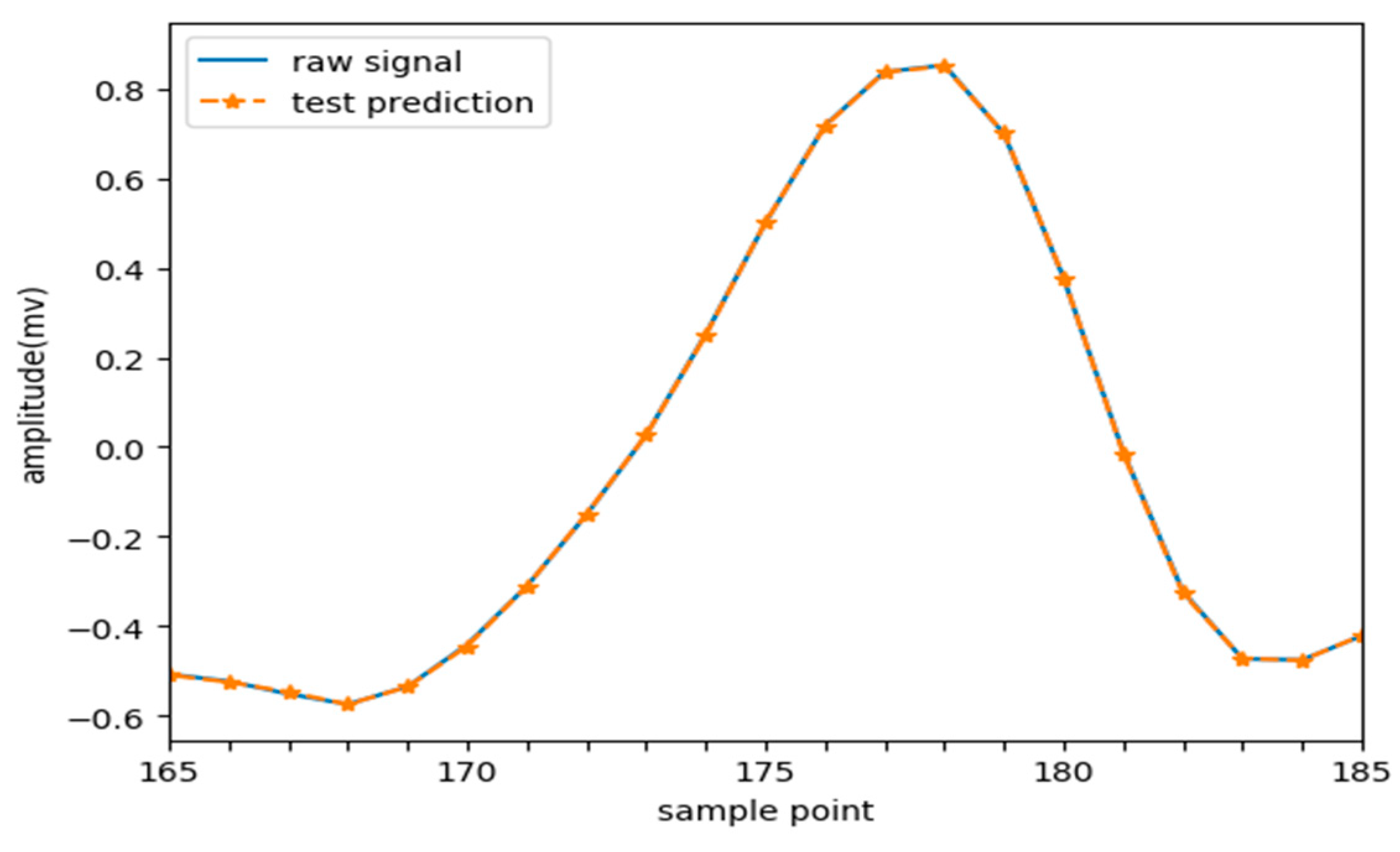
Figure 9.
Comparison of MAE from different prediction methods.
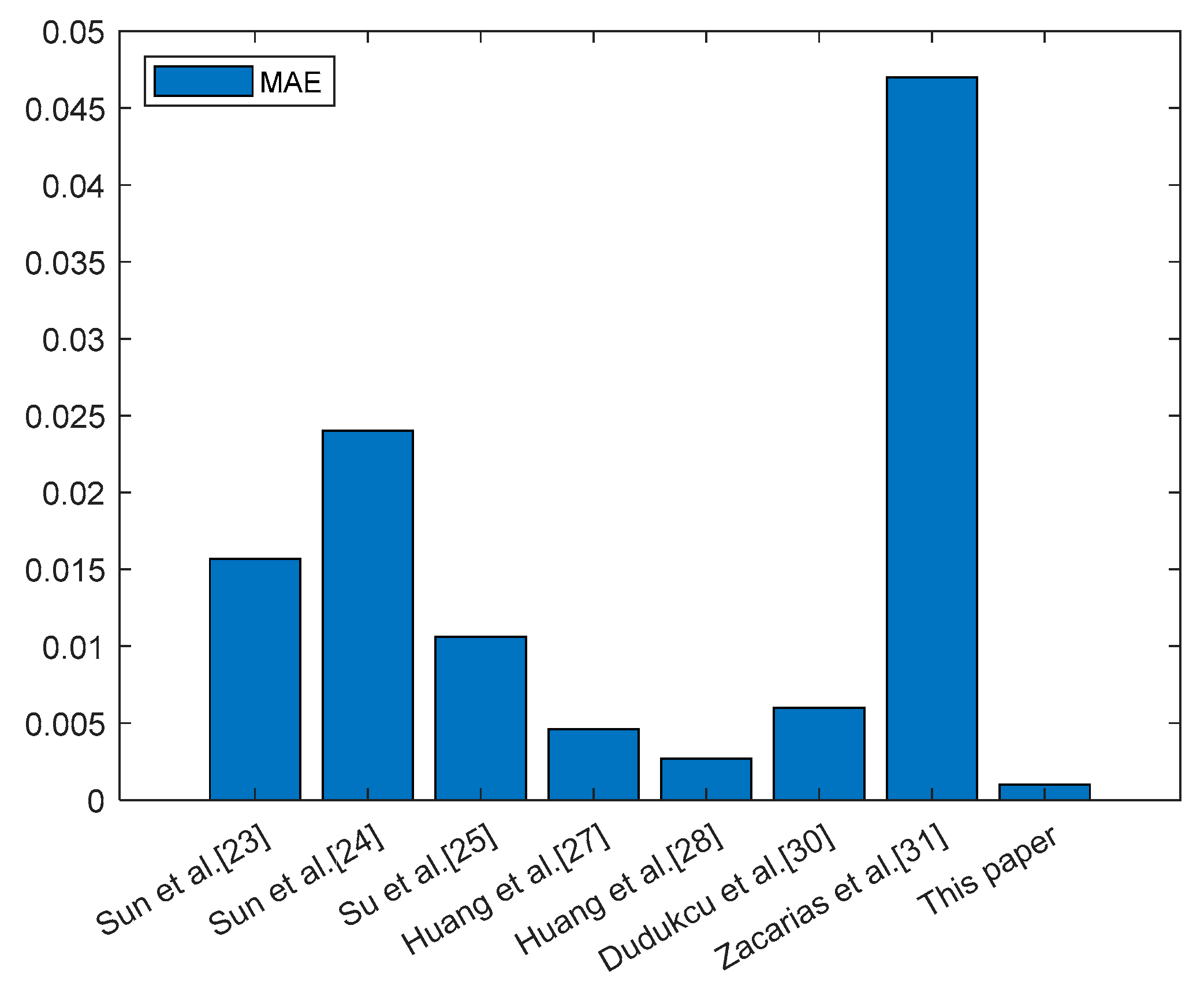
Figure 10.
Comparison of RMSE from different prediction methods.
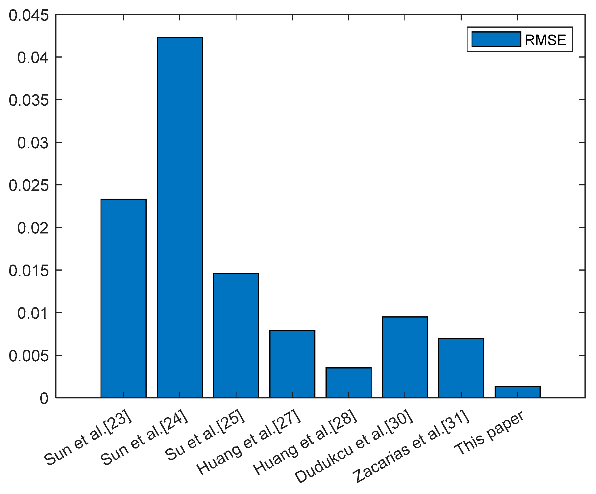
Figure 11.
The box plot of prediction errors in several single deep learning.
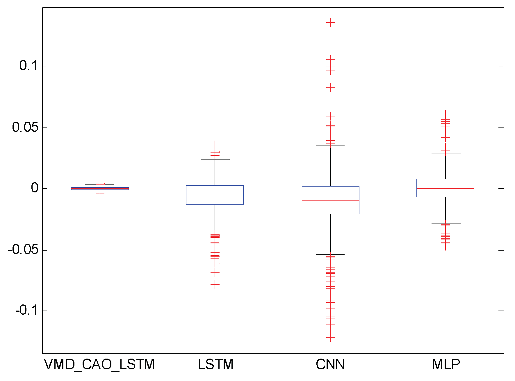

Table 1.
The Rres of VMD with different K.
| K | 1 | 2 | 3 | 4 | 5 | 6 | 7 | 8 | 9 | 10 |
| Rres | 0.0658 | 0.0258 | 0.0116 | 0.0064 | 0.0035 | 0.0021 | 0.0018 | 0.0015 | 0.0018 | 0.0017 |
| K | 11 | 12 | 13 | 14 | 15 | 16 | 17 | 18 | 19 | 20 |
| Rres | 0.0017 | 0.0015 | 0.0016 | 0.0012 | 0.0012 | 0.0011 | 0.0011 | 0.0012 | 0.0012 | 0.0010 |
Table 2.
The embedding dimension of each IMF.
| IMF | 1 | 2 | 3 | 4 | 5 | 6 | 7 | 8 | 9 | 10 | 11 | 12 | 13 | 14 |
| m | 6 | 6 | 6 | 6 | 7 | 6 | 6 | 7 | 10 | 7 | 7 | 8 | 8 | 12 |
Table 3.
Prediction of sliding window approach.
| sliding window | prediction |
Table 4.
Prediction performance of parameter epochs with different values.
| epochs | 100 | 150 | 200 | 250 | 270 | 280 |
| RMSE | 0.002029 | 0.001487 | 0.001396 | 0.001326 | 0.001354 | 0.001484 |
| MAE | 0.001590 | 0.001142 | 0.001065 | 0.001044 | 0.001050 | 0.001154 |
| epochs | 300 | 500 | 1000 | 2000 | 5000 | 10000 |
| RMSE | 0.001504 | 0.001749 | 0.001567 | 0.001427 | 0.001439 | 0.001534 |
| MAE | 0.001143 | 0.001394 | 0.001212 | 0.001125 | 0.001120 | 0.001175 |
Table 5.
Prediction indexes of the test set in No.100 ECG.
| RMSE | MAE | MAPE(%) | R2 |
| 0.001326 | 0.001044 | 0.336560 | 0.999936 |
Table 6.
Comparison of results from different prediction methods.
| Study | Prediction Method | MAE | RMSE |
| Sun et al. [23] | VMD and BPNN | 0.0157 | 0.0233 |
| Sun et al. [24] | MI and BPNN | 0.024 | 0.0423 |
| Su et al. [25] | TS fuzzy model and PSR | 0.0106 | 0.0146 |
| Huang et al. [27] | ARIMA and DWT | 0.0046 | 0.0079 |
| Huang et al. [28] | VMD、PSR and RBFNN | 0.0027 | 0.0035 |
| Dudukcu et al. [30] | TCN-LSTM | 0.0060 | 0.0095 |
| Zacarias et al. [31] | LSTM | 0.0470 | 0.0070 |
| This paper | VMD、Cao and LSTM | 0.0010 | 0.0013 |
Table 7.
Comparison with several popular hybrid prediction methods.
| Prediction method | RMSE | MSE | MAE |
| This paper | 0.001326 | 2.0e-06 | 0.001044 |
| WT-PSR-RBF | 0.0052 | 2.6576e-05 | 0.0031 |
| EMD-PSR- RBF | 0.0128 | 1.6e-04 | 0.0094 |
| VMD-PSR-BP | 0.0174 | 3.0434e-04 | 0.0115 |
| VMD-PSR-GRNN | 0.0126 | 1.5944e-04 | 0.0087 |
Table 8.
Comparison with single deep learning prediction methods.
| Prediction method | This paper | LSTM | MLP | CNN |
| RMSE | 0.001326 | 0.014773 | 0.012900 | 0.026436 |
| MAE | 0.001044 | 0.011094 | 0.009502 | 0.018289 |
Disclaimer/Publisher’s Note: The statements, opinions and data contained in all publications are solely those of the individual author(s) and contributor(s) and not of MDPI and/or the editor(s). MDPI and/or the editor(s) disclaim responsibility for any injury to people or property resulting from any ideas, methods, instructions or products referred to in the content. |
© 2026 by the authors. Licensee MDPI, Basel, Switzerland. This article is an open access article distributed under the terms and conditions of the Creative Commons Attribution (CC BY) license (http://creativecommons.org/licenses/by/4.0/).
Copyright: This open access article is published under a Creative Commons CC BY 4.0 license, which permit the free download, distribution, and reuse, provided that the author and preprint are cited in any reuse.


