
Submitted:
03 February 2026
Posted:
03 February 2026
You are already at the latest version
Abstract
Machine learning is a powerful tool which, when given the availability of comprehensive datasets, required training iterations and the necessary resources to support them, can achieve impressive results in a variety of classification tasks. In this paper, we put forward a
quantum alternative for users that do not posses the ability to gather and store large amounts of data to be used subsequently in lengthy training iterations.
A light-weight probabilistic quantum binary classifier can be built by encoding the two chosen class representatives (images) into
quantum vectors, such that a Principal Component decomposition can express the differences between them only along one dimension
(basis vector). A standard measurement in the computational basis will then project any transformed input sample along one of the two
classes. The classifier accepts quantum representations of images as input, which require exponentially
fewer number of quantum bits compared with the number of classical bits used to store an image.
The technique is illustrated on a "proof of concept" example, in which a quantum character recognizer is built to label any input sample
image as either letter {\bf A} or {\bf P}. The quantum classifier can be tuned to "favor" any of the two classes and the measurement
probabilities follow closely how far an input sample is from the two class representatives. Despite its relative simplicity, the quantum
classifier can distinguish between the standard letter {\bf A} and the standard letter {\bf P} with $98\%$ accuracy. In principle, the procedure
can be applied to any image classification task, including gray-scale and color images, as well as classification problems in which an input
sample is characterized by a collection of properties given by their values.
Keywords:
quantum binary classifier
; quantum image processing
; principal component analysis
; karhunen-loeve decomposition
1. Introduction
Automatic classification of images has become a critical task in many industrial or medicinal applications, particularly in an era where visual information can be captured, stored and processed at rates that seemed unthinkable just a couple of decades ago. Building on these technological advancements, machine learning techniques are proving increasingly successful in tackling problems that require sifting through large number of images. Their success is not based on novel revolutionary approaches (as the fundamentals of machine learning based on neural networks have been developed a long time ago), but it is rather a consequence of our current abilities to acquire and store huge datasets of images on which large AI models can be trained.
The accuracy of these classifiers comes at the cost of many types of resources that are spent to this end: from the raw amount of power required to keep datacenters running (more and more companies are opting to construct their own nuclear plants to support their operations), to the immense computational power required to train AI models and the stress placed on aquifers due to the water consumed to cool these processors. The undeniable advances witnessed in the last few years in many areas of human activity due to ever more powerful AI models are paid for by important environmental consequences, at a time when trying to avert or limit environmental disasters seems increasingly difficult to achieve.
The principles of quantum mechanics, particularly superposition of states, have revolutionized the very foundation of computation, with the promise of an exponential reduction in the number of dimensions used to model many applications, and therefore, a path to achieving a level of scalability that is unmatched in the classical computing paradigm. This is precisely what happens in image classification systems as well, where researchers are trying to reduce the large number of parameters that need to be optimized through training iterations by encoding images into quantum states (hoping to exploit quantum parallelism for enhanced feature extraction) and using hybrid architectures or quantum circuit-based algorithms inspired by classical neural network topologies in order to build the classifier.
The quantum convolutional neural network (QCNN) replaces classical convolution layers with parameterized quantum circuits, but retains significant classical processing for training and inference [1,2,3,4,5]. A typical example in this category is the 2020 paper by Mari et al. [4] proposing a hybrid transfer learning scheme in which a pre-trained classical convolutional network is fit together with a shallow variational quantum circuit in order to perform image classification. The classical backbone extracts rich feature representations from standard benchmark image datasets such as MNIST or CIFAR-10, which are then encoded into a low-depth quantum layer that serves as the trainable classifier. The results reported show that this fusion achieves comparable accuracy with fully classical models, but uses far fewer quantum parameters.
Another example of how variational quantum classifiers can improve hybrid approaches is given in Senokosov et al. [5]. This paper introduces two hybrid quantum–classical neural network architectures for image classification on noisy intermediate-scale quantum (NISQ) devices. The first model employs multiple parallel variational quantum circuits integrated into a classical neural network architecture, while the second model replaces traditional convolutional layers with a “quanvolutional” layer that applies quantum circuits to local image patches before classical processing. The authors report matching classical performance on MNIST and Medical MNIST datasets and exceeding it on CIFAR-10, despite using four times fewer trainable weights. These results underscore the generalizability and parameter-efficiency of quantum layers in image classification tasks.
Unlike the hybrid approaches mentioned above, a less investigated research direction is quantum autoencoders (QAEs). Asaoka and Kudo [6], for example, introduce a fully quantum image-classification framework based on quantum autoencoders, eliminating the need for additional qubits beyond conventional QAE architectures. They explore how different parameterized quantum circuit designs affect classification accuracy under ideal, noise-free conditions using a statevector simulator. Their experiments also achieve accuracy comparable to classical methods while requiring significantly fewer trainable parameters. This work underlines the potential of end-to-end quantum circuits for efficient feature extraction and classification, paving the way for purely quantum machine-learning models on future gate-based hardware.
Regardless of whether their approach is purely quantum or a mixed classical-quantum architecture, the one characteristic relating all current attempts to take advantage of quantum mechanical principles in designing image classifiers is the continued reliance on machine learning techniques, that is going through a series of training iterations in order to adjust a set of parameters ultimately responsible for the performance of the classifier. Although the results obtained through the research efforts mentioned above are promising and the number of training parameters are reduced significantly, they still require a large number of images in the training stage in order to achieve high accuracy classifiers. If the images are quantum encoded first, then there is also the cost of encoding each image as a quantum state before being fed to a quantum learning circuit.
In this paper, we explore a different direction with harnessing quantum principles in order to build quantum image classifiers, without spending a large amount of resources on training. Our interest here lies in assessing the extent to which good light-weight quantum image classifiers can be built based on limited resources. More precisely, we investigate a relatively simple procedure to construct a binary classifier by performing a Principal Component Analysis on the two images designated as class representatives. This avoids the cost of collecting and using a large number of sample images in the training stage, effectively replacing this stage with designing a quantum operator that can aggregate the differences between the two class representatives on a single dimension. Furthermore, the class label produced by the quantum binary classifier is obtained through a simple measurement in the computational basis of the quantum state representing the processed input sample. Our proposed approach may not have the applicability range and the level of accuracy similar to quantum machine-learning approaches, but it provides a recipe for designing binary classifiers that can still achieve good separability with essentially fewer resources (qubits, time, training images, etc.). The method acts on quantum encoded images, which require an exponentially smaller number of qubits to represent and store an image, compared with the number of classical bits needed to achieve the same task.
The remainder of the paper is structured as follows. Next section describes in detail the methodology followed to build a fully quantum binary classifier for a generic image classification problem. Section 3 applies the proposed technique to the concrete problem of classifying input images as either character A or P. A discussion of the performance of the classifier and the parameters that can influence it is given next in Section 4. The paper concludes with a summary of its main contributions together with identifying possible continuations of this research.
2. Methodology
This section describes in detail the approach taken to design a binary classifier for images that are stored and processed through quantum means. The purpose of the binary classifier is to label input samples (images) as belonging to one of two possible classes: Class A or Class B. The steps required to build the classifier are listed below, as Algorithm 1.
| Algorithm 1 Procedure to build a Binary Classifier Through Quantum Means |
|
The main idea of Algorithm 1 is to design a quantum measurement operation that can easily project an input sample, encoded as a quantum state onto one of two possible outputs corresponding to the two possible classes, Class A and Class B. To this end, a class representative that best embodies the main features of its class is chosen for each of the two classes. These two representatives, labeled Img1 and Img2 in Algorithm 1 are then each encoded into a quantum state, denoted as and, respectively, . In general, these two vectors exist in an N-dimensional Hilbert space spanned by the computational basis . The remaining steps (4 through 7) in Algorithm 1 detail a way to construct a quantum measurement operation that will project onto basis vector and onto the subspace spanned by the remaining basis vectors .
In order to achieve this simple separation, first, Step 4 computes the corresponding matrix of a quantum operation that aggregates the differences between the two class representatives and into the inverse amplitudes that the two transformed vectors and share along the first dimension, or basis vector . This matrix, labeled PCM in Algorithm 1, is computed by applying the Karhunen–Loeve decomposition on the two input images, represented as vectors. The Karhunen–Loeve decomposition [7,8] is typically used to reduce the dimensionality of data and capture the most important variation in the first few components, except, in our case, the variation present in Img1 and Img2 is expressed only in the first component of the transformed vectors. In general, the PCM is a linear transformation of the input vectors (Img1 and Img2, in our case), whose columns are the eigenvectors of the covariance matrix formed from Img1 and Img2. The transformed vectors, and are given in order of decreasing variance, and have the same total variance as the input vectors, Img1 and Img2.
The net effect of this Principal Component Quantum Transformation is that it creates two vectors whose amplitudes are identical for all basis vectors except . Dimension 0 is the only one that separates from , with having amplitude along dimension 0 (basis vector ), while has amplitude along the same dimension. Figure 1 gives an intuitive graphical representation of the results produced by the Principal Component Quantum Transformation.
At this point, if a simple computational basis measurement is applied on and , the expected measurement statistics are identical, offering no discrimination between the two sample vectors. However, since the amplitude of term in is negative, an application of the inversion about the average operator used in Grover’s algorithm will boost this amplitude while reducing the corresponding amplitude in . The inversion about the average operator is described by the following matrix:
Depending on the particular vectors chosen as the two class representatives, more than one application of operator may be necessary in order to achieve maximum separation between and . If this is the case, before each application of , the phase of the term is rotated by radians.
Algorithm 1 builds a Quantum Binary Classifier by computing the following two elements: the Principal Component Quantum Transformation that separates the two class representatives along the first dimension (basis vector ) and the optimal number of iterations of Grover’s inversion about the average operator that maximizes the probability of a correct classification through a direct measurement in the computational basis. Based on these two elements, any input sample Img can be labeled as belonging to class A or class B by going through the following steps:
| Algorithm 2 Procedure to classify any input sample image |
|
3. Results
In this section, we exemplify how the methodology described above can be applied on a simple “proof of concept" example, taken from the area of Optical Character Recognition. For the purpose of this example, we have chosen two characters that are not very different, namely P and A. The two images selected as class representatives are depicted below in Figure 2.
A quantum representation has to be chosen now to encode each of these two images into a quantum state. A plethora of possible quantum representations have been proposed over time to encode gray-scale or color images, using either Cartesian or polar coordinates [9,10,11,12,13,14,15,16,17]. In order to represent our black and white images, we settle for a simple representation in which we record for each pixel the x and y coordinates and the "color" (0 for black and 1 for white):
Using this representation, the two quantum states that embody the two images depicting letters P and A are given below:
Applying a Principal Component transformation that aggregates the differences between vectors and along the first dimension (i.e. term ) yields the following transformed vectors, given through the amplitudes of all basis vectors, from to :
Next, we can use the inversion about the average operator in order to be able to distinguish between and through a simple measurement in the computational basis. Applying to will boost the amplitude of the component to , while reducing the corresponding amplitude in to . This means that (representing letter P) has only a chance of being measured as , compared with the approximately probability to measure (representing letter A) as a . For this particular example, using more than one iteration of the inversion about the average operation will not improve the distinguishability between the two characters.
The results above indicate a very different probability of misclassification for the two letters. Since an outcome of in the final measurement labels the input sample as letter A and any other outcome points to an instance of the letter P, there is only a chance that the letter P from Figure 2 will be classified incorrectly as A. On the other hand, letter A from Figure 2 has approximately probability to be labeled as P. In a practical context, if an error in classifying letter P is much more costly than mislabeling instances of letter A, then no corrective action may be necessary. Alternatively, if we want to reduce the error rate for misclassifying A, we can repeat Algorithm 2 several times and identify the sample image as letter A, if any of the last step measurements yields a . For example, if the classification procedure is repeated five times, the chance of mislabeling letter A drops below , while the error rate in classifying letter P increases slightly, remaining below .
Figure 3 shows the probability of misclassifying the two class representatives, for the same number of repetitions of Algorithm 2. The error rate for letter A decreases with the number of repetitions, because more iterations means more chances that one of them will end with a measurement yielding . On the other hand, the misclassification rate for letter P increases with the number of repetitions, because in order for an input image sample to be labeled as P, all iterations must yield a non- outcome in the final measurement step. For the particular case of the two character images chosen for this example, a good compromise is achieved after 12 repetitions, when both error rates are around ( for the letter P and for letter A).
So far, we have discussed the accuracy of our Quantum Classifier in telling apart the two images that were chosen as class representatives for the letters P and A. However, it would be more interesting, perhaps, to test the performance of the classifier on input samples that are different from the two class representatives, particularly images that are somewhere in between the letter P and the letter A. To this purpose, Figure 4 depicts two input image samples representing "incomplete" or "faulty" characters.
Image Sample 1 is almost the standard letter P, with the exception of the top-left pixel, which is white in this image instead of black. On the other hand, the same image is two pixels away from the standard letter A, if the pixels at coordinates and are turned black. Running this Image Sample 1 through Algorithm 2 yields a vector with the following amplitudes before the final measurement in step 4:
According to the amplitudes in state above, there is a probability that Image Sample 1 will be classified as P (non- measurement outcome) and only a chance it will be labeled as character A. Even if we repeat the classification algorithm five times, in an attempt to even out the misclassification rates for the two classes, as discussed above, Image Sample 1 will still be labeled as P (all five measurements yield a non- outcome) of the time. If the number of repetitions is set to 12, then the input will be “recognized" as letter P with probability, which automatically means that there is a chance that Image Sample 1 will be labeled as letter A. The performance of the quantum classifier on Image Sample 1, as a function of the number of repetitions of Algorithm 2, is shown in Figure 5.
Focusing on Image Sample 2 next, we notice that this image is one pixel away from the standard letter A (the bottom-right corner pixel is white instead of black), but at the same time it differs from letter P class representative in just two pixels (the top-left corner pixel and the one at coordinates ). Running Image Sample 2 through the same Algorithm 2 yields the following vector just before the final measurement:
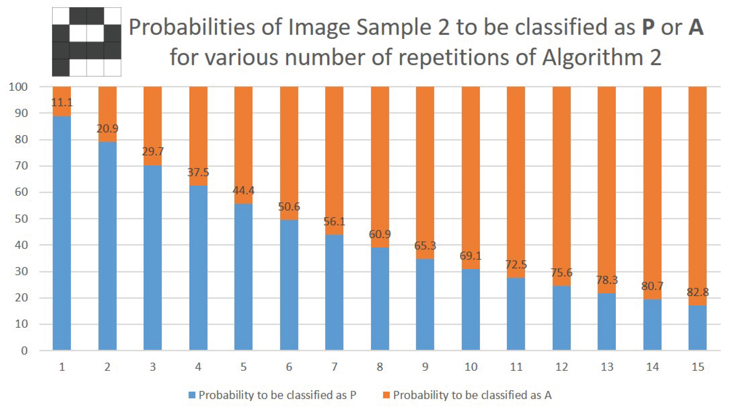
When measured in the computational basis, the above vector has an probability of collapsing on the basis vector. When the procedure is repeated five times, the probability that at least one of the final measurements yields a rises to approximately . In other words, with the number of repetitions set to five, there is a probability that Image Sample 2 is classified as letter A and a probability it will be labeled as letter P. Increasing the number of repetitions to 12 pushes the probability that the input is labeled as A to . The performance of the quantum classifier on Image Sample 2 for various number of repetitions of Algorithm 2 is illustrated in Figure 6.
4. Discussion
The Quantum Image Classifier developed in this paper achieves promising results when applied to the test case of distinguishing two relatively close images, depicting the letters P and A. As seen in Figure 3, the classifier can be “tuned" to recognize any of the two letters with very high success rate (around ). This happens when the number of repetitions of Algorithm 2 is set to 12.
The number of times Algorithm 2 is applied is an important parameter of our classifier, allowing the user to skew the performance of the classifier either towards class A or class B. A small number of repetitions favors an input image to be classified as belonging to class A, while a larger number of repetitions will increase the chance that the input is labeled as an instance of class B. Such a tuning parameter may be useful in practical binary classification tasks to control the number of false positives vs. false negatives. The optimal number of repetitions, that will result in a balanced classifier, will certainly depend on the particular characteristics of the task for which the classifier is built. For the particular character recognition task that served as a test case for our quantum classifier methodology, the optimal number of repetitions seemed to be 12.
An important property exhibited by the proposed quantum classifier, particularly given its simple design employing a projective measurement onto the computational basis vectors, is robustness. The results depicted in Figure 5 and Figure 6 attest to the fact that, even if the input sample is "borderline" between the two classes (both Image Sample 1 and Image Sample 2 are just one pixel closer to one of the two classes, compared to the distance to the other one), the classifier still labels the sample as belonging to the "closer" class, with overwhelming probability.
The last point we wish to make pertains to the applicability of the methodology described herein to build a purely quantum binary classifier. Although the technique was illustrated on a simple classification problem, in order to be able to present all technical details and go through the necessary calculations, the procedure can be applied to any binary classification task of images belonging to two different classes, including gray-scale and color images. Quantum representations of such images have been proposed in the literature [11,16,17,18] and they can be used to encode each class representative into a quantum state, such that Algorithm 1 can then proceed as described.
Furthermore, the vectors encoding the class representatives may not be restricted to represent only images. In general, they can be representations of "objects" described by any number of properties, such as position in space, shape, color, texture, mass, temperature, etc. The normalized values for these properties can be encoded into a quantum vector using superposition of states and then the PCM matrix could be computed.
5. Conclusions
In a world increasingly characterized by the fierce competition among state actors or big tech companies for AI dominance, the necessary resources to achieve this dominance are critical. The ever higher number of data centers that are vital to AI functions incur a lot of pressure on local communities in terms of land utilization, water consumption, power availability or rising energy prices.
In this context, the current manuscript explores the idea of using quantum information processing techniques in order to construct good performance classifiers that are using significantly fewer resources, albeit quantum resources, compared with typical machine learning techniques that entail large data sets and many iterations to train the classifier.
To illustrate our approach, we provided a "proof of concept" example in which we built a fully quantum binary classifier that can label an input sample as either letter A or P. The classifier accepts quantum representations of images as input, which require exponentially fewer number of quantum bits compared with the number of classical bits used to store an image.
Building the quantum binary classifier amounts to computing a quantum transformation on the state space in which the two vectors chosen as class representatives live. This linear transformation, calculated based on the Karhunen–Loeve decomposition, essentially performs a Principal Component Analysis in which the variations between the two input vectors are expressed along the first dimension (basis vector ). Experiments show that a standard measurement in the computational basis can distinguish between the two classes, with good probability, even for input samples that are borderline cases between the two class representatives, attesting to the classifier’s robustness.
Once the classifier is built, applying it repeatedly on multiple copies of an input image may act as a parameter that can tune the performance of the classifier towards recognizing samples of a particular class with arbitrarily high accuracy, at the expense of correctly classifying samples from the other class.
The framework presented in this paper opens up a novel direction of research in the general field of quantum AI. We are looking forward to future developments in the area of light-weight quantum classifiers that may uncover new practical applications in concrete domains of human activity.
Supplementary Materials
The Wolfram Mathematica code used to simulate the Quantum Binary Classifier and the experimental results presented in Section 3 (Results) is available at https://github.com/madi12c/Quantum-Binary-Classifier/
Funding
This research received no external funding.
Data Availability Statement
Not applicable to this article as no datasets were generated or analyzed during the current study.
Conflicts of Interest
The authors declare no conflicts of interest.
Abbreviations
The following abbreviations are used in this manuscript:
| AI | Artificial Intelligence |
| QCNN | Quantum Convolutional Neural Network |
| NISQ | Noisy Intermediate-Scale Quantum |
| QAE | Quantum AutoEncoder |
References
- Cong, I.; Choi, S.; Lukin, M.D. Quantum Convolutional Neural Networks. Nature Physics 2019, 15, 1273–1278. [Google Scholar] [CrossRef]
- MacCormack, I.; Delaney, C.; Galda, A.; Aggarwal, N.; Narang, P. Branching Quantum Convolutional Neural Networks. Physical Review Research 2022, 4, 013117. [Google Scholar] [CrossRef]
- Song, Y.; Li, J.; Wu, Y.; Qin, S.; Wen, Q.; Gao, F. A Resource-Efficient Quantum Convolutional Neural Network. Frontiers in Physics 2024, 12, 1362690. [Google Scholar] [CrossRef]
- Mari, A.; Bromley, T.R.; Izaac, J.; Schuld, M.; Killoran, N. Transfer learning in hybrid classical–quantum neural networks. Quantum 2020, 4, 340. [Google Scholar] [CrossRef]
- Senokosov, A.; Sedykh, A.; Sagingalieva, A.; Kyriacou, B.; Melnikov, A. Quantum machine learning for image classification. Machine Learning: Science and Technology 2024, 5, 015040. [Google Scholar] [CrossRef]
- Asaoka, H.; Kudo, K. Quantum autoencoders for image classification. Quantum Machine Intelligence 2025, 7, 71. [Google Scholar] [CrossRef]
- Stark, H.; Woods, J.W. Probability and Random Processes with Applications to Signal Processing, 4th ed.; Pearson Education: Upper Saddle River, NJ, 2012. [Google Scholar]
- Bishop, C.M. Pattern Recognition and Machine Learning; Springer: New York, 2006. [Google Scholar]
- Le, P.Q.; Dong, F.; Hirota, K. A flexible representation of quantum images for polynomial preparation, image compression, and processing operations. Quantum Information Processing 2011, 10, 63–84. [Google Scholar] [CrossRef]
- Khan, R.A. An Improved Flexible Representation of Quantum Images. Quantum Information Processing 2019, 18, 1–19. [Google Scholar] [CrossRef]
- Sun, B.; Iliyasu, A.M.; Yan, F.; Dong, F.; Hirota, K. An RGB Multi-Channel Representation for Images on Quantum Computers. JACIII 2013, 17, 404–417. [Google Scholar] [CrossRef]
- Zhang, Y.; Lu, K.; Gao, Y.; Wang, M. NEQR: a novel enhanced quantum representation of digital images. Quantum Information Processing 2013, 12, 2833–2860. [Google Scholar] [CrossRef]
- Caraiman, S.; Manta, V.I. Image processing using quantum computing. 2012 16th International Conference on System Theory, Control and Computing (ICSTCC), 2012; pp. 1–6. [Google Scholar]
- Zhang, Y.; Lu, K.; Gao, Y.; Xu, K. A Novel Quantum Representation for Log-polar Images. Quantum Information Processing 2013, 12, 3103–3126. [Google Scholar] [CrossRef]
- Li, H.S.; Zhu, Q.; Song, L.; Shen, C.Y.; Zhou, R.G.; Mo, J. Image storage, retrieval, compression and segmentation in a quantum system. Quantum Information Processing 2013, 12, 2269–2290. [Google Scholar] [CrossRef]
- Li, H.S.; Zhu, Q.; Zhou, R.G.; Song, L.; jiang Yang, X. Multi-dimensional color image storage and retrieval for a normal arbitrary quantum superposition state. Quantum Information Processing 2014, 13, 991–1011. [Google Scholar] [CrossRef]
- Liu, X.; Zhou, R.G. Color Image Storage and Retrieval Using Quantum Mechanics. Quantum Information Processing 2019, 18, 1–14. [Google Scholar] [CrossRef]
- Sang, J.; Wang, S.; Niu, X.; Wang, J. A novel quantum representation of color digital images (NCQI). Quantum Information Processing 2017, 16, 42. [Google Scholar] [CrossRef]
Figure 1.
Principal Component Visual Representation.
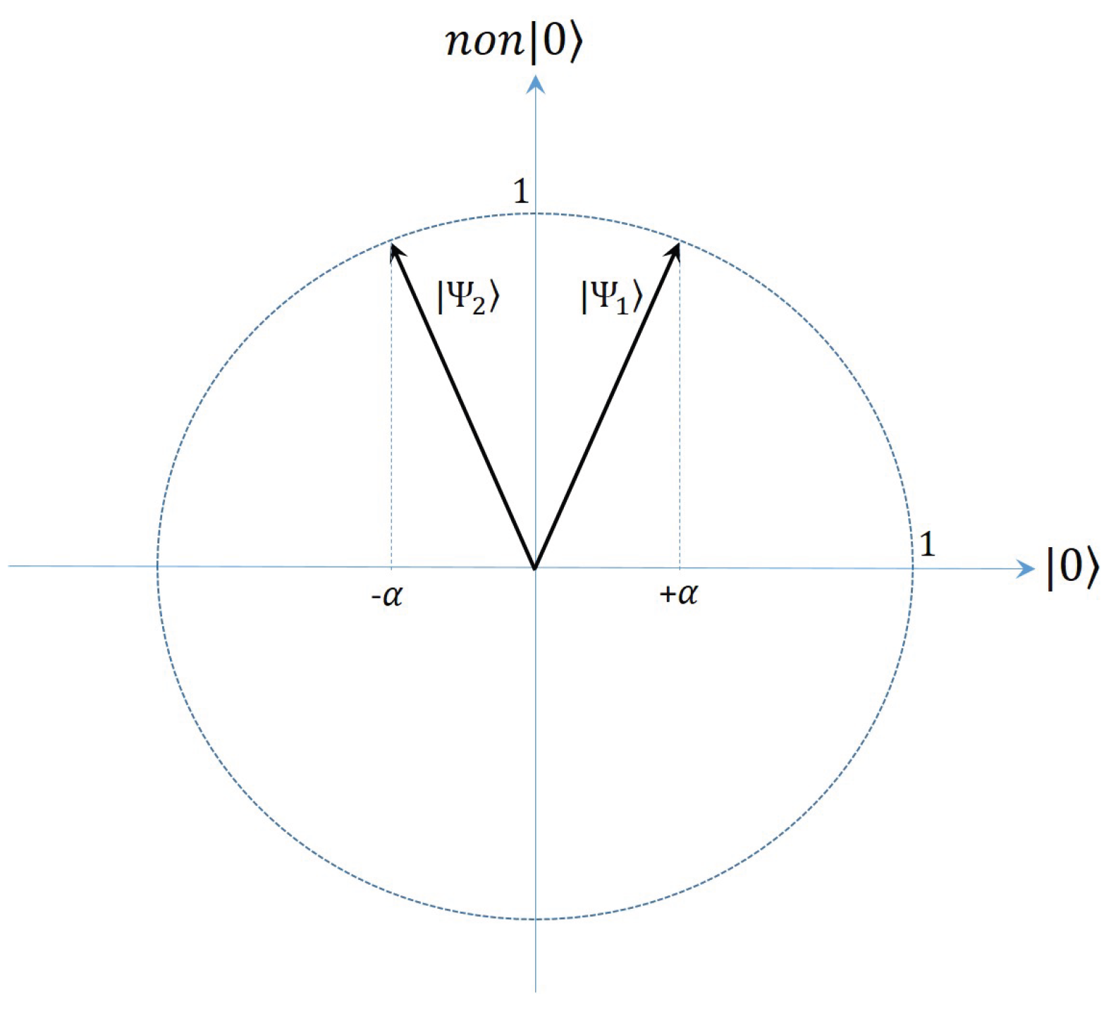
Figure 2.
Class Representatives for characters P and A.
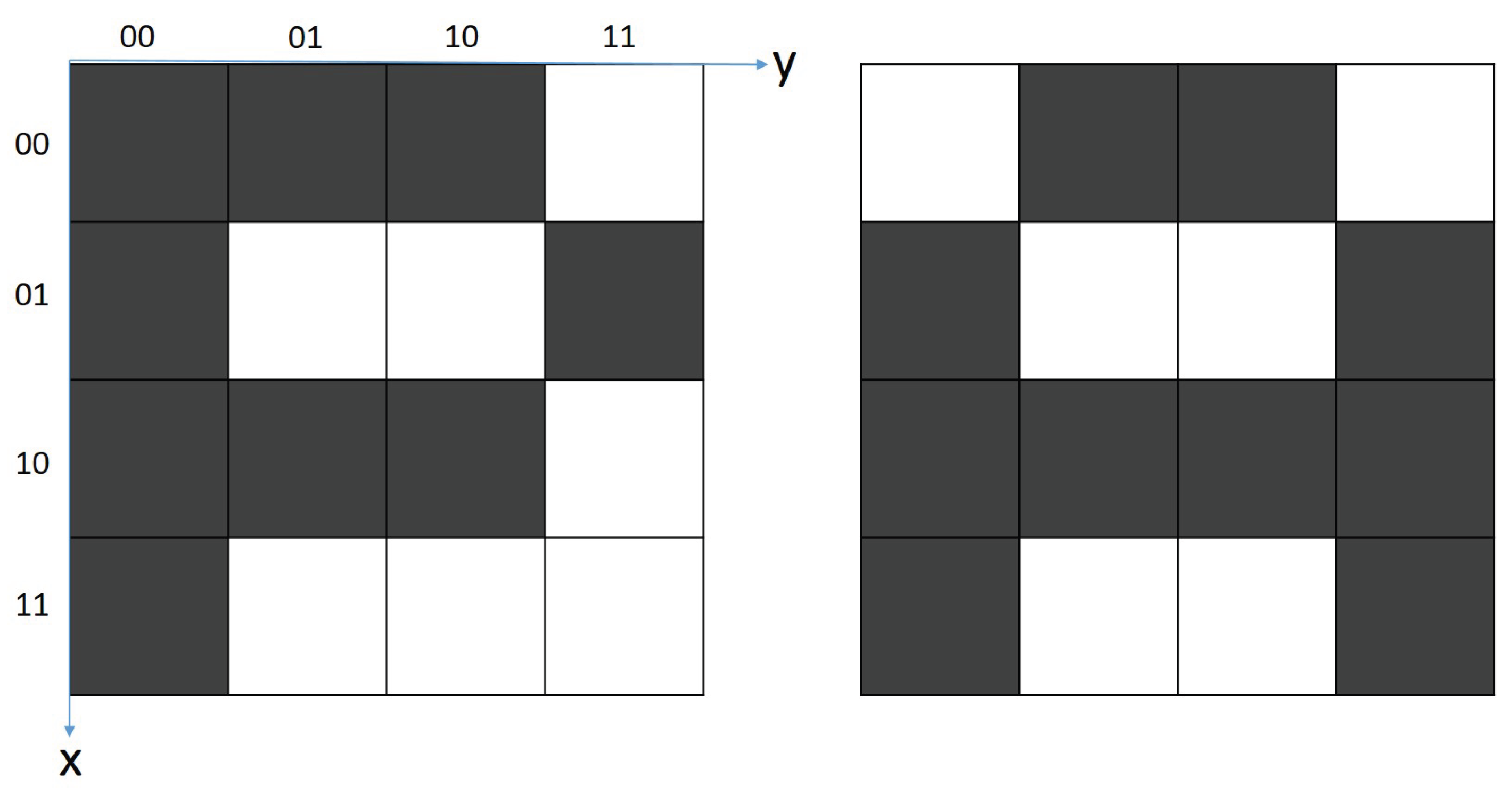
Figure 3.
Misclassification rates for characters P and A for various number of repetitions of Algorithm 2. For example, if the classification procedure is repeated five times, the chance of mislabeling letter A drops below , while the error rate in classifying letter P increases slightly, remaining below . A good compromise is achieved after 12 repetitions when both error rates are around .
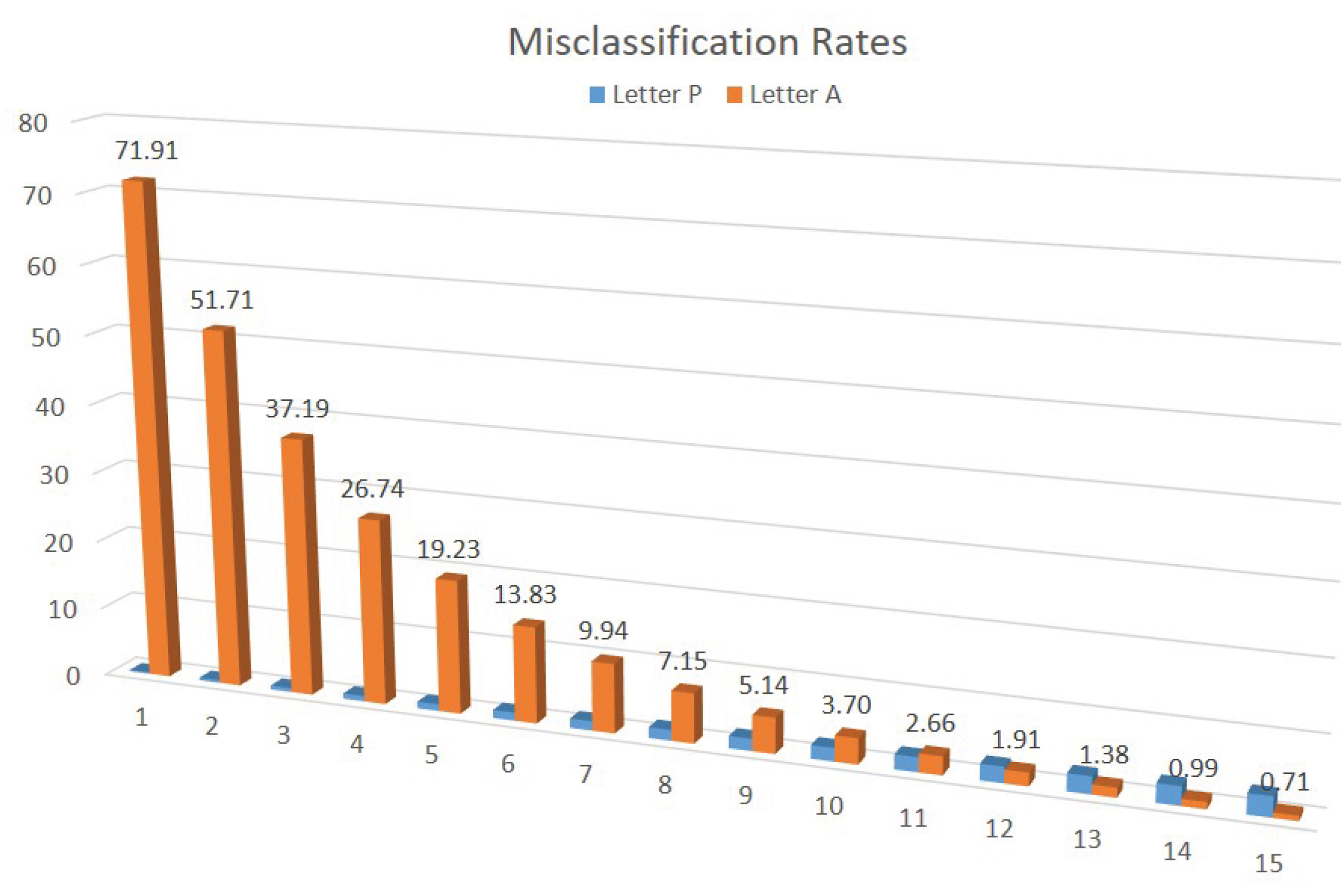
Figure 4.
Input image samples representing "faulty" characters somewhere between P and A.
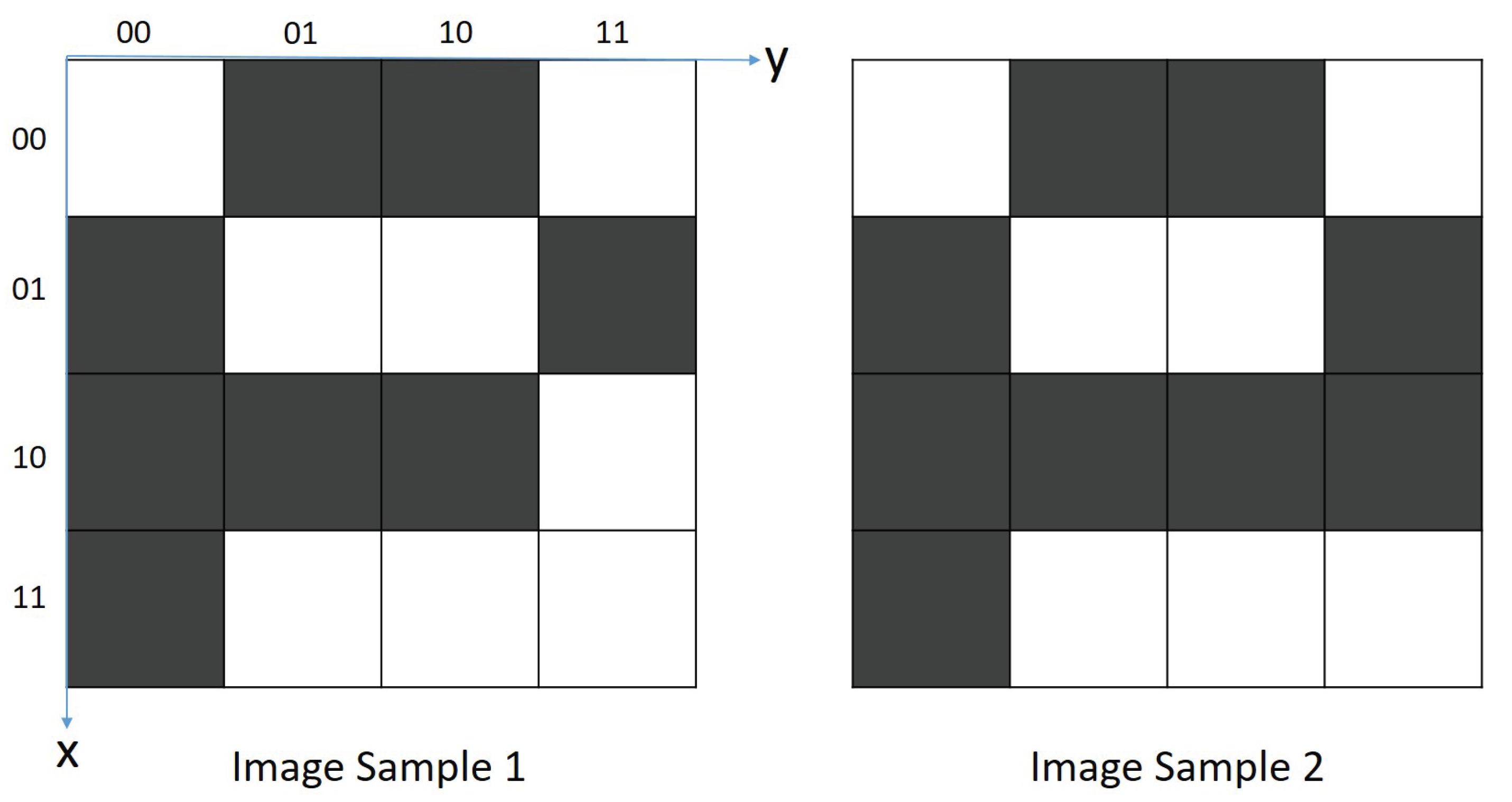
Figure 5.
Probabilities that Image Sample 1 (depicted in the top left corner) will be classified as letter P or A based on the number of times Algorithm 2 is applied. After 12 repetitions there is an chance the sample is “recognized" as P and a probability it will be classified as A.
Figure 5.
Probabilities that Image Sample 1 (depicted in the top left corner) will be classified as letter P or A based on the number of times Algorithm 2 is applied. After 12 repetitions there is an chance the sample is “recognized" as P and a probability it will be classified as A.
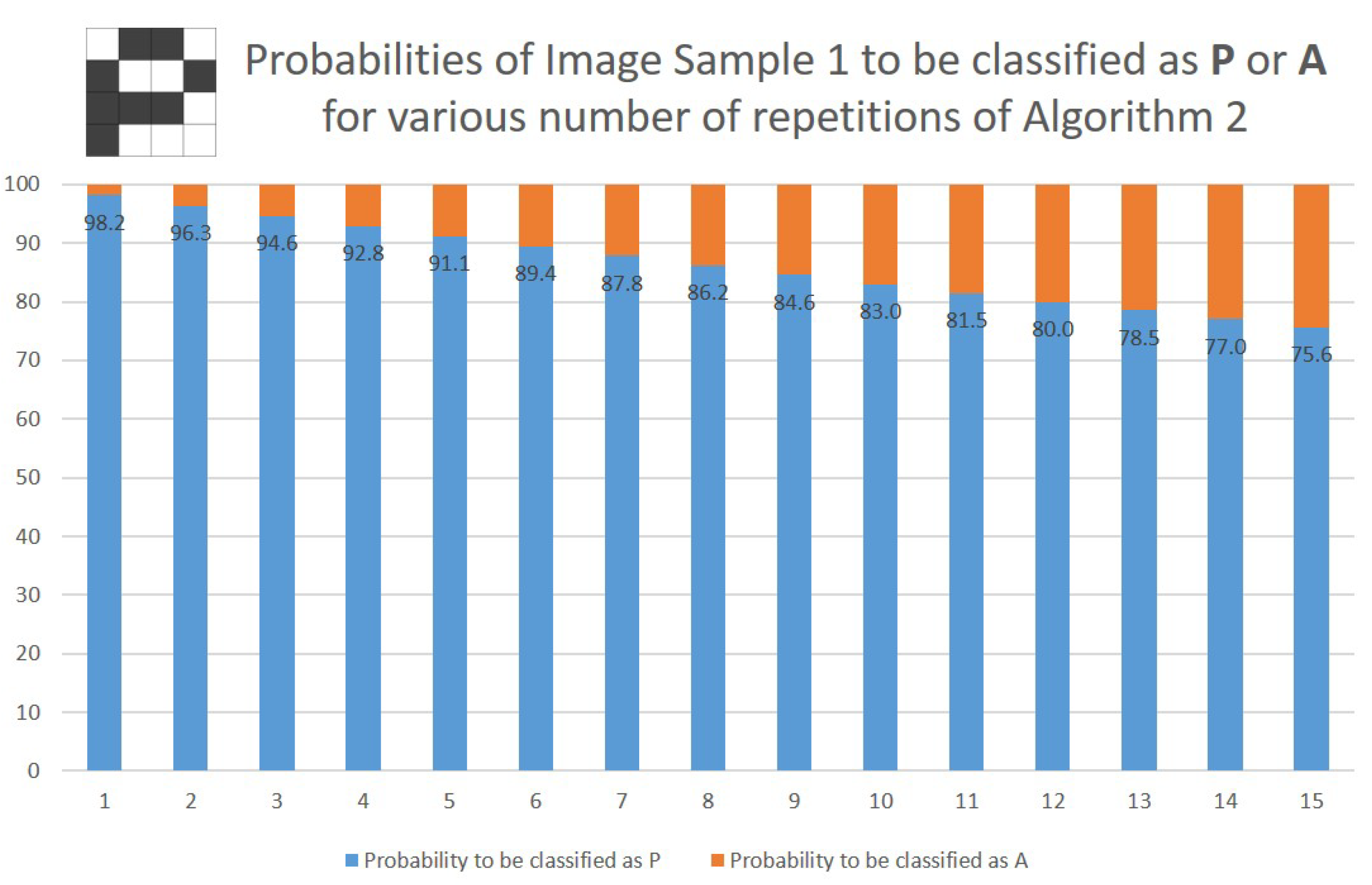
Figure 6.
Probabilities that Image Sample 2 (depicted in the top left corner) will be classified as letter P or A based on the number of times Algorithm 2 is applied. After 12 repetitions there is an chance the sample is “recognized" as P and a probability it will be classified as A.
Figure 6.
Probabilities that Image Sample 2 (depicted in the top left corner) will be classified as letter P or A based on the number of times Algorithm 2 is applied. After 12 repetitions there is an chance the sample is “recognized" as P and a probability it will be classified as A.
Disclaimer/Publisher’s Note: The statements, opinions and data contained in all publications are solely those of the individual author(s) and contributor(s) and not of MDPI and/or the editor(s). MDPI and/or the editor(s) disclaim responsibility for any injury to people or property resulting from any ideas, methods, instructions or products referred to in the content. |
© 2026 by the authors. Licensee MDPI, Basel, Switzerland. This article is an open access article distributed under the terms and conditions of the Creative Commons Attribution (CC BY) license (http://creativecommons.org/licenses/by/4.0/).
Copyright: This open access article is published under a Creative Commons CC BY 4.0 license, which permit the free download, distribution, and reuse, provided that the author and preprint are cited in any reuse.


