Submitted:
02 February 2026
Posted:
03 February 2026
You are already at the latest version
Abstract
We propose and analyze a new class of copulas (generated by two univariate functions) that exhibit asymmetric nonlinear dependence, resulting from an antisymmetric perturbation of the independence copula. Within this framework, we construct a parametric subclass of asymmetric copulas for which we derive the analytical expression of Kendall’s tau (τ). We present properties related to asymmetry and dependence measures, and provide several examples. To the best of our knowledge, this novel feature of our class represents a significant advancement in the context of the most studied perturbed copulas, which have been recently the focus of numerous scientific investigations.
Keywords:
copula
; perturbation
; concordance measure
; asymmetry measures of concordance
1. Introduction
Copulas are mathematical tools and objects that capture and model the dependence structure between random variables by constructing (bivariate for instance, or multivariate) distributions with given marginal distributions. Consider a two-dimensional random vector with joint distribution function and continuous margins and . There exists a copula C such that:
Here, C is nothing other than the distribution function of the vector , where and are uniform random variables on . Thus, copulas allow us to describe the dependence structure between X and Y independently of their marginal distributions. They have gained significant importance and popularity in various fields, such as finance, insurance, risk management, reliability theory, and other disciplines (see [1,2,3,4,5]).
Over the years, a large number of copula families and various methods for their construction have been proposed and studied. For instance, see some works that have inspired our research ([6,7,8,9,10,11,12]).
Our study focuses on a bivariate copula construction principle based on modifying a known copula (particularly the independence copula, denoted by , where ) by adding a factorial term to its expression. We are thus interested in copulas that can be expressed as :
where P is a continuous function on the unit square with values in , called the "perturbation factor". In this case, the copula C is referred to as a perturbation of by means of P.
P can be interpreted as a disruption of independence (see Durante et al. [6]).
This type of construction underlies several copula families. For example, we may cite the well-known Farlie–Gumbel–Morgenstern FGM family, given by:
Several extensions of this family, along with their properties, have recently been studied by Saminger-Platz et al. [13]. When the perturbation P is not symmetric, we refer to [12] where a new family of asymmetric copulas is detailed.
The paper is organized as follows : We begin by reviewing the definitions, properties, and key results concerning copulas, which are central to our analysis. Next, we describe a particular class of asymmetric copulas based on a slight perturbation of the product copula , while providing necessary and sufficient conditions on the generating functions of this perturbation. Subsequently, we examine the main dependence property characterizing this copula family, relying on a specific class of weak concordance measures for bivariate copulas recently studied by Mesiar et al. [14] - which encompasses most well-known concordance measures in the literature. Finally, we investigate and quantify the asymmetry of our new copula class.
2. Preliminaries
In this contribution, for the sake of simplicity, only bivariate copulas will be considered and treated, they will simply be referred to as copulas.
Definition 1.
A function is called a copula if it satisfies the following two conditions :
- 0 and 1 are, respectively, its zero element and identity argument, i.e.
- 2-increasing, i.e., for all where and , the volume over the rectangle
Remark 1.
- 1.
- The condition (3) maybe compactly written
- 2.
- If C has second derivatives, then the 2-increasing property (4) is equivalent to
In what follows, we denote by the set of all (bivariate) copulas, and let . The set possesses many interesting properties, such as being a closed convex subset of the set of functions from the unit square to the unit interval. The Fréchet-Hoeffding bounds W (the countermonotonicity copula) and M (the comonotonicity copula) are respectively its smallest and largest elements, given by : and . Furthermore, , C is increasing in each variable, i.e, and for all and and is also 1-Lipschitz, i.e., for all . It is also invariant under strictly increasing transformations.
Each copula can be decomposed into a sum of an absolutely continuous component and a singular component , given respectively by:
when , we say that C is absolutely continuous.
Note that any absolutely continuous copula can be represented as a perturbation of (see [6]).
Let us now recall the involutive operations on the set of all two-dimensional random vectors and their connections with respective involutive operations on the set .
- The transformation corresponds to the involutive transformation ,
- The transformation corresponds to the involutive transformation ,
- The transformation corresponds to the involutive transformation ,
- The transformation corresponds to the involutive transformation ,
- The transformation corresponds to the involutive transformation ,
- The transformation corresponds to the involutive transformation .
Note that is called the transpose, the first flipping, the second flipping, and is a survival operation.
The analysis of transformations applied to copulas constitutes an active research field (see [18]).
In cases where:
- , C is called symmetric,
- , C is called radially symmetric.
The latter cas was intensively investigated in [19], where invariance of a copula under the transformation was deeply discussed.
Example 1.
- 1.
- , Every member of the FGM family given by (2), is both symmetric and radially symmetric,
- 2.
- The Fréchet copulas , are also both symmetric and radially symmetric.
Theorem 1.
A copula is symmetric if and only if there exists a copula C such that
It is extremely easy to see that for any symmetric copula S we have: . However, what appears more interesting is the inverse problem. This leads us to the fundamental question :
Given a symmetric copula S, do there exist other asymmetric copulas satisfying the equality ? In this regard, the authors of [12] have provided an answer to this problem for some notable copulas: and .
Proposition 1.
- (i)
- M is the unique copula C satisfying ;
- (ii)
- W is the unique copula C satisfying ;
- (iii)
- There exist numerous copulas C satisfying
Proof.
- (i)
- Let C be a copula such that , then . We thus obtain two functions and one negative and the other positive, which are equal. This allows us to conclude that , hence the uniqueness.
- (ii)
- The same reasoning as above applies.
- (iii)
-
For this proposition, they only proposed a parametric family of asymmetric copulas satisfying (6), given by:.
□
Our study proposes a new class of families of copulas satisfying (6), which means the copulas whose symmetrized version is identical to the product copula . The following result can be easily obtained.
Proposition 2.
Let , be a continuous function. Then, C defined by satisfying (6) is a copula, if and only if the following conditions hold:
- (i)
-
.(i.e, ),
- (ii)
- ,
- (iii)
- for all rectangle .
In other words: The perturbation P must satisfy three requirements:
First, it must vanish on the boundaries of . Secondly, it must be antisymmetric. Thirdly, the amount of negative mass that it can add to each rectangle of is bounded by the positive mass given by .
Remark 2.
Note that any copula C naturally defines a probability measure on . If C takes the form (1), the measure of a rectangle R decomposes into the sum of the measures induced by Π and P.
In what follows, we express the above characterization under specific hypotheses by selecting appropriate functions.
3. New Class of Copulas Based on Antisymmetric Perturbations
3.1. Characterization of the New Class of Copulas
We focus here on copulas whose representation can be formulated as follows:
where: are two non-zero continuous functions. In other words, we have chosen naturally the perturbation .
This form provides a flexible method for introducing new copula families by selecting appropriate functions f and g.
We now need to establish and identify the necessary and sufficient conditions to guarantee that the function defined by (7) is indeed a copula. To achieve this, we begin by stating and proving the following preliminary lemma
Lemma 1.
Let be two non-zero continuous functions, and a non-zero function defined by . Then the following two propositions are equivalent:
- (i)
- ,
- (ii)
- .
Proof.
The implication is obvious, we therefore focus on the converse.
From we have , and we then obtain:
We assume that at least one of the two functions f and g does not vanish at 0. In this regard, we distinguish two cases.
-
If exactly one of the two functions does not vanish at 0, this means that or .For and with , the hypothesis implies that , therefore, , which is absurd (since g is considered as a continuous non-zero function. i.e, there exists such that ). The same reasoning applies to the other case : and with .
-
If both functions do not vanish at 0, then there exist two nonzero real numbers and such that with , substituting the last two equalities into (8), we find that: , where . Hence, , this is impossible since P is assumed to be non-identically zero.Thus, .
By following the same steps as above for equation (9), we obtain: . In addition, one may deduce the second point in the Lemma 1 by considering the functions and .
It follows that, . □
We are now in a position to state and prove the central theorem of this section.
Theorem 2.
Let be two non-zero continuous functions, the function given by (7) is a copula, if and only if the following conditions hold
- (1)
- ,
- (2)
- f and g are absolutely continuous,
- (3)
- .
Proof.
Note that the equivalence of the first condition of Theorem 2 with the boundary conditions (3) is a direct consequence of Lemma 1. Moreover, we have (if there exists) is equivalent to . Consequently, conditions and lead to conclude that C is 2-increasing.
Conversely, suppose that C is a copula, for each such that and , the function formed, respectively, by the horizontal sections of C and at is absolutely continuous for all (see [20]). There thus exists such that , where
Therefore,
Hence, .
By hypothesis (), we obtain
Hence the absolute continuity of f, as a linear combination of two absolutely continuous functions ( and ). A similar reasoning allows us to conclude that g is also absolutely continuous.
The third property of the theorem follows immediately from (4), the proof is thus completed. □
Let and .
In the case where: and with , , and . we have, , so the third condition of Theorem 2 becomes in this case
Example 2.
Let and ,
So, and ,
Then, and ,
Hence, and ,
From (10) we have then, ,
It folows that: defines a copula.
Example 3.
Let and ,
So, and ,
Then, and ,
Hence, and ,
It follows that, ,
Thus, be a copula.
3.2. Subclass and Some Examples
We introduce in this section a parametric subclass of copulas derived from formulation (7), which will be the subject of a more detailed characterization later in our work.
Corollary 1.
Let C be the function given by (7) with , where
. Then we obtain:
is a copula if and only if the following conditions hold:
- (i)
- ,
- (2)
- f and g are absolutely continuous,
- (3)
- .
Proof.
The proof is a matter of simple computations of the derivatives for the third condition of Theorem 2. □
Note that The function g plays a role similar to the generating function in Archimedian copulas see [16], and the inclusion of the coefficient ensures the validity of the copula construction, and its range depends only on the choice of the function g.
We now propose a few examples of functions g generating parametric families of copulas. One of these examples will be used to illustrate antisymmetry and to evaluate Kendall’s tau in the following sections.
Example 4.
Let m and n be two non-null real numbers such that , and let g be the function defined by: , then if and if .
For and
We have, ,
For and
We find that, ,
For and
,
For and
We have, .
Thus,
is a copula, where .
Example 5.
For where .
We have, . Then,
Hence, ,
Thus, ,
is a copula, where .
Remark 3.
We can easily see that our subclass serves to perturb any member of the semiparametric family of symmetric copulas introduced and studied by Rodrıguez-Lallena and Úbeda-Flores [8], is given by
which includes the Farlie–Gumbel–Morgenstern family as a particular case.
Let , then , hence . Moreover, we have , therefore . According to Corollary 1
it follows that
A convex combination of the two parametric families of copulas (15) and (14) (the case where ) generates, for every , the parametric family of copulas expressed by
where and .
Each copula of the FGM family can thus be perturbed by a convex combination with a copula that belongs to our parametric subclass, thus providing a richer modeling tool for capturing complex dependence structures observed in real data.
3.3. Illustrations
We conclude this section with a few plots to visualize the shapes of the two previous examples. More precisely, we provide the 3D surfaces and contour plots for the copulas previously defined in (12) and (13), as well as for their corresponding perturbation factors P.
As an illustration, we have chosen the parameters characterizing the copula defined in (12) as and , whereas for the copula defined in (13) see Figure 1.
These visualizations make it possible to analyze how the perturbations modify the dependence structure between the variables, by highlighting the deviations from the independence case.
The 3D representations in Figure 1 display slightly curved hyperbolic surfaces compared to the independence copula , suggesting a weak dependence introduced by the two perturbations. Regarding the contour plots, their deviations from the copula are subtle, they are not symmetric with respect to the diagonal , reflecting the asymmetry of the two proposed examples.
Note that the larger the parameters m and n, the weaker the perturbation, bringing the perturbed copula closer to the independence copula.
4. Properties of the New Subclass
4.1. Preliminaries on Measures of Concordance
Let and be two continuous random vectors, if the corresponding copulas are and .
then the function Q defined by:
is called the concordance function, it was introduced by [21]. Its probabilistic representation is given by:
This function has several properties, among which we mention the following:
- Symmetry, ,
-
Monotonicity in each argument, (meaning that a stronger concordance ordering between copulas implies a higher concordance value),Formally, if and , then
-
The concordance function Q remains unchanged when the copulas are replaced by their survival copulas or by their transposes, while it changes sign when they are replaced by their reflections:For more details, see [18]
In [22], Scarsini offers a characterization of concordance measures as mappings that assign a real number to each copula C, in accordance with axioms set forth in the following definition.
Definition 2.
A function is called a concordance measure if it satisfies the following conditions:
- ,
- ,
- ,
- where , then ,
- If a sequence of copulas converges uniformly to , then .
Since the independence copula is invariant under both reflections, and by condition , we deduce that
The four most frequently used concordance measures, which also play a central role, are: Kendall’s , Spearman’s , Gini’s and Blomqvist’s .
When condition is replaced with the normalization condition (17), we obtain what Liebscher [23] calls a weak concordance measure. Spearman’s footrule is a typical example of such a weak measure of concordance (see [24]).
Note that the set of all weak concordance measures covers all concordance measures.
A (weak) concordance measure is said to be convex, if it satisfies the following property:
wich can be seen as the linearity of applied to convex combinations of copulas. Let defined by : .
is a convex concordance measure if and only if is a linear function, i.e, . Equivalently, it means that is of degree 1 in the sense of Edwards and Taylor [25].
To simplify the statements, we will henceforth use the term concordance measure to refer to the five studied measures.
The first four concordance measures can be expressed in terms of the concordance function Q.
- Kendall’s : ,
- Spearman’s : ,
- Gini’s : ,
- Spearman’s footrule : ,
- On the other hand, Blomqvist’s is given by:
Example 6.
For every , the four dependence measures ρ, τ, β and γ associated with FGM copulas given by (2) are linear functions of the parameter θ.
Furthermore, these parameters exhibit simple proportional relationships:
the ranges of these measures for any , are given by:
4.2. Single Point-Generated Convex Weak Concordance Measures
We now turn our attention to a concordance measure whose values depend on the symmetrized copula given previously by (5). This measure encompasses several well-known (weak) convex concordance measures from the literature, including Spearman’s Rho, Gini’s Gamma, Blomqvist’s Beta, and Spearman’s Footrule.
Since all copulas coincide on the boundary of the unit square, we consider a point . The fact that is a symmetric copula implies that and , this allows us to focus only on points within the set . Given any fixed point , the mapping is increasing, i.e., , we have , and consequently, . We can therefore normalize into as follows:
Based on the above considerations, we introduce an alternative formulation for the family of convex concordance measures generated by a single point, recently proposed in [14].
Theorem 3.
Let . The function given by:
is a weak convex concordance measure.
Proof.
By construction, we immediately observe that: and . Moreover, for all , if , then uniformly for each . From our earlier discussion, the other axioms of weak concordance measures (invariance under permutation and boundedness on ) are easily verified.
Regarding the convexity of : and ,
Thus, is convex. We omit the detailed calculations. □
Remark 4.
For
which yields ,
which confirms that there is no lower bound for convex weak concordance measures.
Example 7.
For any fixed point we have:
When , we obtain the Blomqvist , i.e., .
4.3. Representation of Basic Weak Convex Concordance Measures via and
Any convex combination of (weak convex) concordance measures remains a (weak convex) concordance measure. Formally:
let be weak convex concordance measures. The function defined by: where with is also a concordance measure. This can be interpreted as a Lebesgue integral with respect to a probability measure defined on (the Borel subsets of I) by , i.e,
Theorem 4.
Let P be a probability measure defined on , then the mapping given by :
is a convex weak concordance measure.
Proof.
The proof of this statement is similar to that of Theorem3. □
Moreover, note that there exists a probability measure on such that, for each copula , we have, where and are the weak convex concordance measures given in (19) and (20) respectively.
See ([14], Theorem 4.1)
Proposition 3.
Let P and Ψ be two probability measures on , with respective densities p and ψ.
-
If and , ,then, (Spearman’s ρ),
-
IfAnd,where, and ,then, (Gini’s γ).
-
Ifand,then, (Spearman’s footrule ϕ).
Proof.
- •
-
Considering the probability measure on with density , as . Then the corresponding convex weak concordance measure introduced in (19) can be determined as follows:The same result can be obtained by using the representation exprimed in (20).
- •
-
Let be a probability measure on whose support is the set and densityThen
- •
- The support of probability measure , is the set . We directly obtain
□
4.4. Dependence Properties
For every copula D belonging to our new subclass of copulas of the form (11), we trivially observe that . This result follows directly from the characterizing property (6) of this subclass. It follows that the classical concordance measures — ( and ) vanish identically.
Regarding Kendall’s tau, its expression is established in the proposition below.
Let us recall that by applying integration by parts to the expression of Kendall’s defined by
We obtain an alternative formulation that is more convenient for numerical computation:
Furthermore, if the copula C is absolutely continuous, then:
Where, denotes the copula density of C.
For more detail, we refer to [16].
Proposition 4.
Let be a random pair whose copula is given by (11). We have:
Kendall’s τ admits the following representation:
Proof.
The partial derivatives of the copula
are expressed by
Analogously, we find that:
First, we deduce that the Kendall’s can be expressed as the sum of four terms:
On the one hand, we have:
consequently,
On the other hand,
where, by integration by parts, we have:
thus,
□
It is not surprising that Kendall’s tau behaves differently from the other concordance measures — , and . This dissimilarity is explained by the linearity of the latter under convex combinations, whereas Kendall’s exhibits a quadratic behavior.
Example 8.
We revisit the copula generated by the function , where , as given by (13), for different values of the shape parameter n, which controls the concentration of mass around , as shown in Figure 2.
Figure 2 also illustrates the evolution of , whose graph displays three curves, each corresponding to a specific value of n and its associated . The vertical dashed lines indicate the value of for each n.
- For , is the largest (approximately 0.1133).
- For the other two cases, and , decreases (approximately 0.0769 and 0.0219, respectively).
Consequently, the larger the value of n, the smaller the value of θ, and the lower the maximum value of . These observations are consistent with the behavior of the function g, as n increases, g becomes more concentrated around and vanishes more rapidly elsewhere, which leads to a reduction in .
We now study a partial order on . Let and be two copulas. is said to be more concordant than , denoted , if (see [16]). Let and be two copulas such that and , where and , then , if and only if,
The following two theorems consider continuous random pairs associated with the copula and characterize the pairs that satisfy certain well-known positive dependence properties.
In what follows, we will use some concepts of positive dependence (for more details, see [16]). A copula C is said to be positively quadrant dependent () if , and negatively quadrant dependent () if . It should be noted that copulas exhibiting this property concentrate more mass near the main diagonal than near the opposite diagonal.
For our own parametric family of copulas given by (11), we have the following result, the proof of which is straightforward.
Theorem 5.
Let and be a continuous random pair associated with the copula given by (11). Then X and Y are PQD , if and only if either g(u) and g(v) have the same sign , or g(u) and g(v) have opposite signs .
The interconnections between the dependence properties described in the following and a probabilistic interpretation of these relationships are discussed in [26]. For this, each concept of positive dependence studied in the following theorem implies PQD. We may therefore assume, without loss of generality, that the generating function g is concave with , which allows us to deduce that
And that g is symmetric with respect to . Consequently, for all , and . Under these considerations, we find that is PQD .
This result is perfectly illustrated by (Figure 1, (b) and (d)), which provide a particularly insightful graphical representation of it.
Theorem 6.
Let and be a continuous random pair associated with the copula given by (11), where g is a concave function with . Then:
- Y is left tail decreasing in X (), if and only if , for almost all u, and holds, if and only if either and or , for almost all v.
- Y is right tail increasing in X (), if and only if either and or , for almost all u, and () holds, if and only if, , for almost all v.
- Y is stochastically increasing in X (), if and only if and () holds, if and only if .
Proof.
- 1.
-
According to (corollary 5.2.6,nelsen2006introduction), holds if and only if, for anyThus, we have: .And .The inequality (28) therefore becomes , by rearranging the terms, and from (27), we obtain .Let (an affine function with respect to v).If , this implies that is increasing, consequently, reaches its maximum at .Hence, is equivalent to for almost all u.If , this implies that is decreasing, hence reaches its maximum at .Therefore, is equivalent to which contradicts for almost all u.Similarly, for . Following the same steps as before, we find thatthis leads to .Let .If , which implies that is increasing, hence reaches its minimum at .Then is equivalent to for almost all v.If , then is decreasing, consequently reaches its minimum at .Thus, is equivalent to for almost all v.
- 2.
-
holds if and only if, for any ,this leads to .Let .If , then reaches its maximum at . is equivalent to for almost all u.If , then reaches its maximum at .Then, is equivalent to for almost all u. (where ).can be proved using similar arguments.
- 3.
-
holds if and only if, for any , is a concave function of u.We haveThen , implies thatLet , since .This leads to is increasing, i.e, reaches its maximum at .Hence is equivalent to .The same reasoning applies to , hence the result.
□
4.5. Tail Dependence
Tail dependence quantifies the joint likelihood of extreme events in a bivariate distribution’s tails (see [3]).
Let X and Y be continuous random variables with respective distribution functions F and G. The upper and lower tail dependence coefficients are respectively
and,
According to ([16], Theorem 5.4.2). If the limits exist, the upper and lower tail dependence coefficients and can also be characterized in terms of the copula associated with the joint distribution of . Let denote the copula of the pair . Then:
and
Proposition 5.
The copula of the form (11) has a total tail independence, i.e,
5. Asymmetry Analysis of Our New Class of Family of Copulas
In this section, we analyze the asymmetry of copulas belonging to our new family through the relationships between an asymmetry measure (non-exchangeability), denoted by , and the four convex concordance measures and , recently introduced by Bukovšek et al. [27].
The topic of asymmetry or non-exchangeability of copulas has recently received considerable attention and plays a prominent role in current research [28,29,30,31].
A function is called a measure of asymmetry (or non-exchangeability) for a copula C if it satisfies the following properties:
- There exists such that for all , we have ,
- if and only if, (C is symmetric),
- ,
- If and C are in , if converges uniformly to C, then converges to .
As an example, a broad class of asymmetry measures was proposed by Nelsen [32], for a complementary reference, see [33].
Let denote the classical distance on for . For all .
- •
- For :
- •
- For :
The measure is then defined as , and can be normalized using , see [34].
Property implies the continuity of with respect to the topology induced by the norm on and the euclidean norm on . The compactness of therefore guarantees the existence of a maximum for , which justifies the existence of the following result.
Proposition 6.
Let for , be a measure of asymmetry. Then, there exists a constant and a copula such that, , and for all copula .
Proof.
According to result ([32], Lemme 2.1), for any copula C and any , we have:
by integrating both sides of this inequality over the unit square, we obtain, :
□
Note that and
Now choose such that : . From the convexity of , it readily follows that there exists a copula satisfying
We adopt the notation to denote the positive part of x.
Theorem 7.
Proof.
If , by the 1-increasing property, we have .
If , by the 1-Lipschitz property, we obtain
hence, it follows that
Similarly, by the same properties. It follows that
If , then .
If , then ,
consequently,
In a manner analogous to the previous one, we find that
This leads us to
hence, , where .
Incorporating the Fréchet-Hoeffding bounds completes the proof. □
An alternative proof, structured around five distinct cases according to the regions defined by the scatterplots, is developed in ([27], Theorem 2)
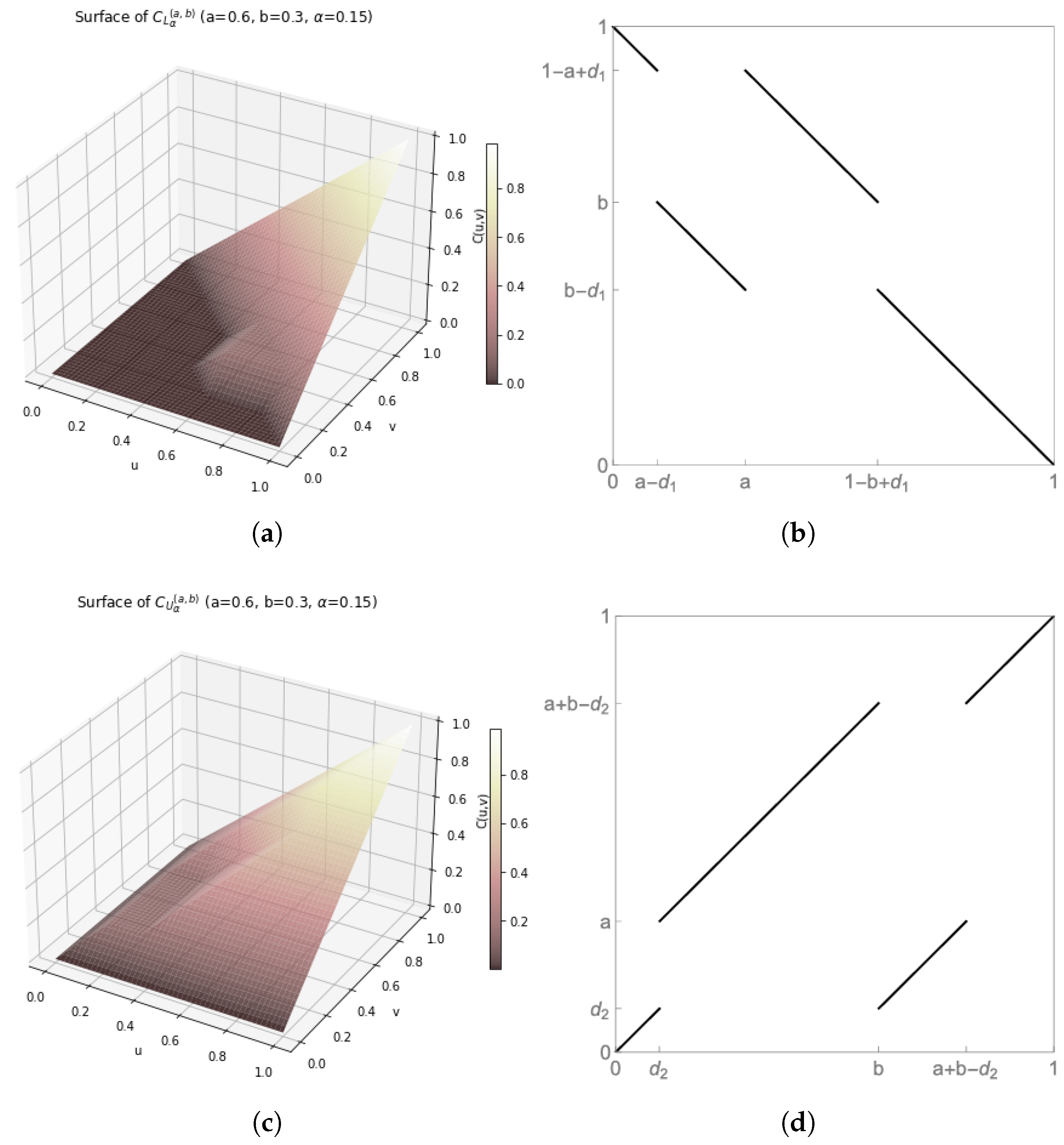
The calculation of the concordance measures for the local Fréchet-Hoeffding bounds, defined respectively by (32) and (33), requires the evaluation of the concordance function Q (given by (16)) applied to these two copulas, as well as to and M. The synthesis of the graphical observations (Figure 3) and the preliminary calculations then reveals that
and
In accordance with ([27], Properties 4 and 5), through which the authors derive formulas (36) and (37) for every , the results obtained are symmetric with respect to both the main diagonal and the counter-diagonal. i.e,
Let and .
and
Let be any copula with , there exists a pair such that
then, (If we replace C with ).
By virtue of Theorem 7, it follows that
as an immediate consequence of monotonicity, we have
Given the symmetries discussed in (38) and (39), we fix m. The study can therefore be restricted to the set without loss of generality.
The analysis is therefore limited to the triangle with the vertices and .
It results that
Following ([27], Corollary 22), the minimum value of and the maximum value of on the set are attained at the same point, denoted and , respectively. The preceding developments make it possible to establish the link between the measure and each measure .
Theorem 8.
•
Let be any copula with . Then
In particular,
For , we have , where
For , we have , where
For , we have , where
And
For , we have , where
And
Note that, If copula C takes the maximal possible asymmetry . Then
and .
Regarding our new class of family of copulas, the use of inverses immediately yields the following result.
Corollary 2.
Let C be the copula satisfying the property (6),
- If , then .
- If , then .
- If , then .
- If , then .
Remark 5.
for all copula . If , then C takes the maximal possible asymmetry . See [32]. The inductive inference, based on the data from Figure 2, reveals that for any copula C belonging to the parametric family given by (13), we have
Let C be a copula of the form , where , we have . The corollary 2 directly implies that: .
Which appears to be a good indicator of the mildness of the perturbation.
6. Conclusion and Directions for Further Research
This article defines and studies a class of parametric antisymmetric copula families and establishes their dependence and asymmetry properties. The methodology developed for the analysis of concordance and dependence measures relies on a family of Convex weak concordance measures, allowing the inference of a nonlinear dependence structure characterizing the considered copula class. This, in turn, provides an optimal modeling framework for various phenomena in which weak dependencies reveal critical nonlinear structures.
In line with our previous approach, our future work will consist in characterizing and analyzing a family of copulas arising from an anti-radially symmetric perturbation of the independence copula. It is worth noting that this perturbative approach is extensible to the multivariate case, which will be addressed separately in future work.
Another research direction is to identify and study another class of copulas whose symmetrized part is Archimedean.
Funding
This research received no external funding.
Institutional Review Board Statement
Not applicable.
Informed Consent Statement
Not applicable.
Data Availability Statement
Not applicable.
Acknowledgments
The authors would like to thank the anonymous referees for their insightful comments and suggestions, which led to significant improvements in the manuscript.
Conflicts of Interest
The authors declare no conflicts of interest.
Abbreviations
The following abbreviations are used in this manuscript:
| FGM | Farlie-Gumbel-Morgenstern |
| PQD | Positively Quadrant Dependent |
| LTD | Left Tail Decreasing |
| RTI | Right Tail Increasing |
| SI | Stochastically Increasing |
References
- Blier-Wong, C.; Cossette, H.; Marceau, E. Risk aggregation with FGM copulas. Insurance: Mathematics and Economics 2023, 111, 102–120. [CrossRef]
- Kupka, I.; Kisel’ák, J.; Ishimura, N.; Yoshizawa, Y.; Salazar, L.; Stehlik, M. Time evolutions of copulas and foreign exchange markets. Information Sciences 2018, 467, 163–178. [CrossRef]
- De Kort, J. Modeling tail dependence using copulas-literature review. Faculty of Electrical Engineering, Mathematics and Computer Science (EEMCS), Delf University of Technology 2007.
- Oussama, E.; Mohamed, E.; Ahmed, S. An analytic treatment of evolution copulas. Asia Pacific Journal of Mathematics 2024.
- Yoshizawa, Y.; Ishimura, N. Evolution of multivariate copulas in continuous and discrete processes. Intelligent Systems in Accounting, Finance and Management 2018, 25, 44–59. [CrossRef]
- Durante, F.; Sánchez, J.F.; Flores, M.Ú. Bivariate copulas generated by perturbations. Fuzzy Sets and Systems 2013, 228, 137–144. [CrossRef]
- Komorník, J.; Komorníková, M.; Kalická, J. Dependence measures for perturbations of copulas. Fuzzy Sets and Systems 2017, 324, 100–116. [CrossRef]
- Rodrıguez-Lallena, J.A.; Úbeda-Flores, M. A new class of bivariate copulas. Statistics & probability letters 2004, 66, 315–325.
- Amblard, C.; Girard, S. A new extension of bivariate FGM copulas. Metrika 2009, 70, 1–17. [CrossRef]
- Mesiar, R.; Komorníková, M.; Komorník, J. Perturbation of bivariate copulas. Fuzzy Sets and Systems 2015, 268, 127–140. [CrossRef]
- Manstavičius, M.; Bagdonas, G. A class of bivariate independence copula transformations. Fuzzy sets and systems 2022, 428, 58–79. [CrossRef]
- Mohamed, E.; Ahmed, S. New asymmetric perturbations of FGM bivariate copulas and concordance preserving problems. Moroccan J. of Pure and Appl. Anal.(MJPAA) 2023.
- Saminger-Platz, S.; Kolesárová, A.; Šeliga, A.; Mesiar, R.; Klement, E.P. The impact on the properties of the FGM copulas when extending this family. Fuzzy Sets and Systems 2021, 415, 1–26. [CrossRef]
- Mesiar, R.; Kolesárová, A.; Sheikhi, A.; Shvydka, S. Convex weak concordance measures and their constructions. Fuzzy Sets and Systems 2024, 478, 108841. [CrossRef]
- Trivedi, P.K.; Zimmer, D.M.; et al. Copula modeling: an introduction for practitioners. Foundations and Trends® in Econometrics 2007, 1, 1–111.
- Nelsen, R.B. An introduction to copulas; Springer, 2006. [CrossRef]
- Durante, F.; Sempi, C.; et al. Principles of copula theory; Vol. 474, CRC press Boca Raton, FL, 2016. [CrossRef]
- Fuchs, S.; Schmidt, K.D. Bivariate copulas: transformations, asymmetry and measures of concordance. Kybernetika 2014, 50, 109–125. [CrossRef]
- El maazouz, M.; Sani, A. Stability of copulas under survival transform. Electronic Journal of Mathematical Analysis and Applications 2022, 10, 115–123.
- Klement, E.P.; Kolesárová, A.; Mesiar, R.; Sempi, C. Copulas constructed from horizontal sections. Communications in Statistics—Theory and Methods 2007, 36, 2901–2911. [CrossRef]
- Kruskal, W.H. Ordinal measures of association. Journal of the American Statistical Association 1958, 53, 814–861.
- Scarsini, M. On measures of concordance. Stochastica 1984, 8, 201–218.
- Liebscher, E. Copula-based dependence measures. Dependence Modeling 2014, 2.
- Spearman, C. Footrule for measuring correlation. British Journal of Psychology 1906, 2, 89.
- Edwards, H.; Taylor, M. Characterizations of degree one bivariate measures of concordance. Journal of multivariate analysis 2009, 100, 1777–1791. [CrossRef]
- Fuchs, S.; Tschimpke, M. Total positivity of copulas from a Markov kernel perspective. Journal of Mathematical Analysis and Applications 2023, 518, 126629. [CrossRef]
- Bukovšek, D.K.; Košir, T.; Mojškerc, B.; Omladič, M. Relation between non-exchangeability and measures of concordance of copulas. Journal of Mathematical Analysis and Applications 2020, 487, 123951. [CrossRef]
- Siburg, K.F.; Stehling, K.; Stoimenov, P.A.; Weiß, G.N. An order of asymmetry in copulas, and implications for risk management. Insurance: Mathematics and Economics 2016, 68, 241–247. [CrossRef]
- Fernandez-Sanchez, J.; Ubeda-Flores, M. On degrees of asymmetry of a copula with respect to a track. Fuzzy Sets and Systems 2019, 354, 104–115. [CrossRef]
- Karbil, L.; Maazouz, M.E.; Sani, A.; Daoudi, I. Asymmetry quantification in cross modal retrieval using copulas. J. Math. Comput. Sci. 2022, 12. [CrossRef]
- De Baets, B.; De Meyer, H.; Jwaid, T. On the degree of asymmetry of a quasi-copula with respect to a curve. Fuzzy Sets and Systems 2019, 354, 84–103. [CrossRef]
- Nelsen, R.B. Extremes of nonexchangeability. Statistical Papers 2007, 48, 329–336. [CrossRef]
- Durante, F.; Klement, E.P.; Sempi, C.; Úbeda-Flores, M. Measures of non-exchangeability for bivariate random vectors. Statistical Papers 2010, 51, 687–699. [CrossRef]
- Beliakov, G.; De Baets, B.; De Meyer, H.; Nelsen, R.; Úbeda-Flores, M. Best-possible bounds on the set of copulas with given degree of non-exchangeability. Journal of Mathematical Analysis and Applications 2014, 417, 451–468. [CrossRef]
Figure 1.
(a) 3D and contour plots of copula given by (12) with and . (b) 3D and contour plots of factor perturbation P of copula C given by (13) with and . (c) 3D and contour plots of copula given by (12) with . (d) 3D and contour plots of factor perturbation P of copula C given by (13) with .
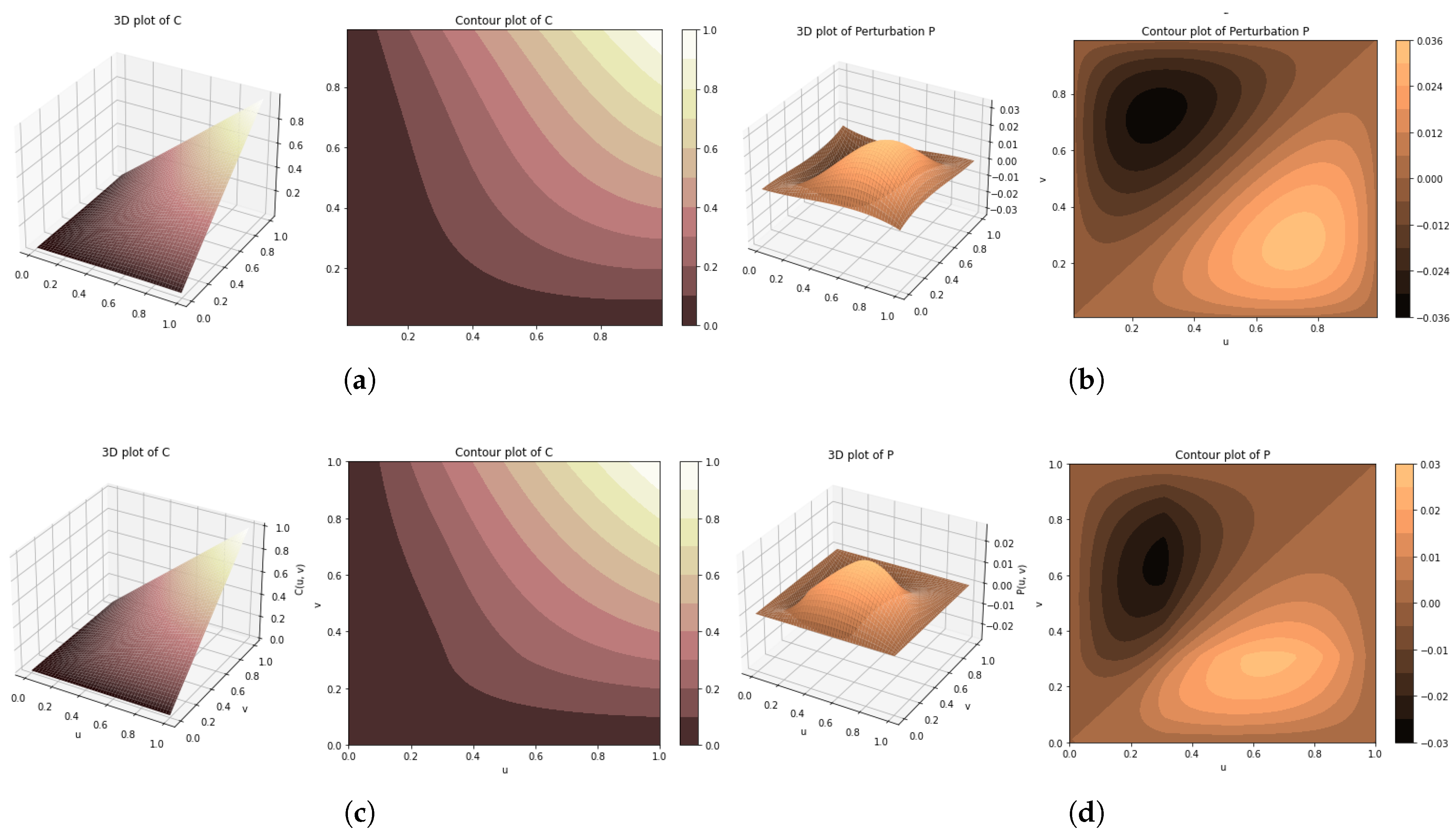
Figure 2.
The evolution of Kendall’s tau for the copula defined by (13), over the set of values .
Figure 2.
The evolution of Kendall’s tau for the copula defined by (13), over the set of values .
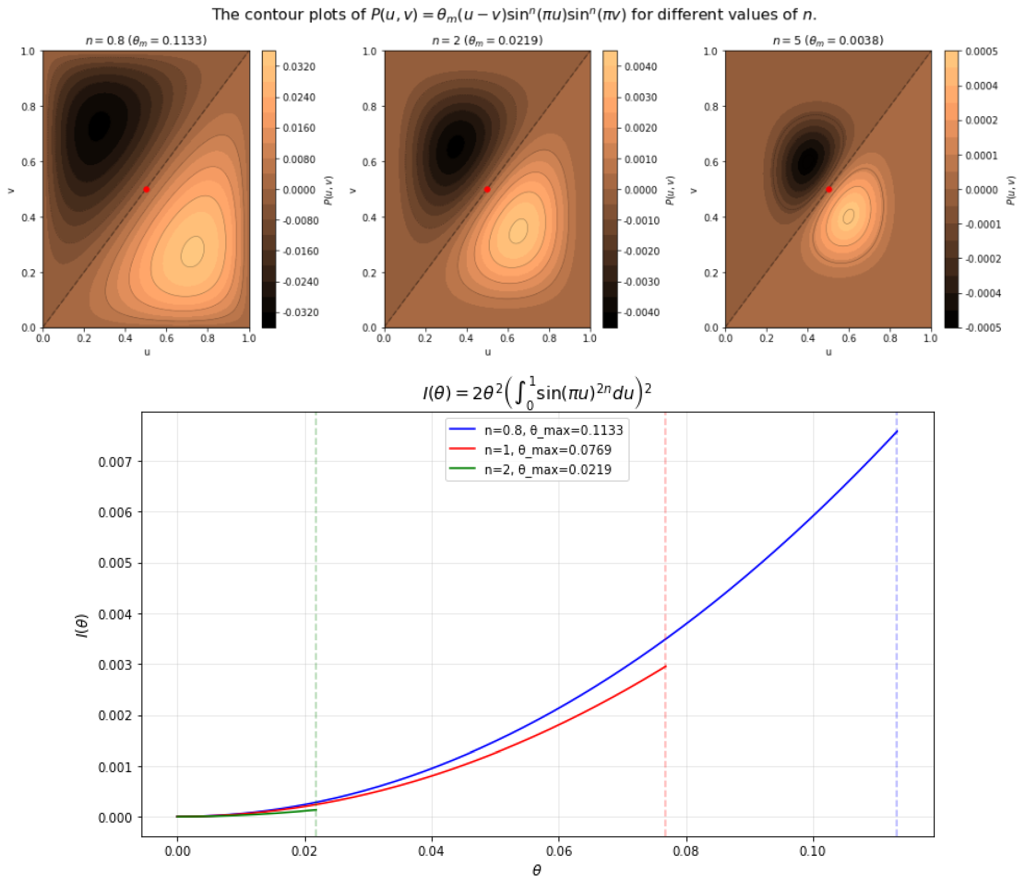
Figure 3.
(a) and (c) The respective 3D representations of and . (b) and (d) their scatter plots.
Disclaimer/Publisher’s Note: The statements, opinions and data contained in all publications are solely those of the individual author(s) and contributor(s) and not of MDPI and/or the editor(s). MDPI and/or the editor(s) disclaim responsibility for any injury to people or property resulting from any ideas, methods, instructions or products referred to in the content. |
© 2026 by the authors. Licensee MDPI, Basel, Switzerland. This article is an open access article distributed under the terms and conditions of the Creative Commons Attribution (CC BY) license (http://creativecommons.org/licenses/by/4.0/).
Copyright: This open access article is published under a Creative Commons CC BY 4.0 license, which permit the free download, distribution, and reuse, provided that the author and preprint are cited in any reuse.


