Submitted:
01 February 2026
Posted:
03 February 2026
You are already at the latest version
Abstract
We present a systematic geometric analysis of sectional curvature structures on fibred Calabi-Yau manifolds using the theory of Riemannian submersions and O'Neill's curvature decomposition formulas. Emphasis is placed on elliptic, toroidal, and K3 fibrations arising in complex dimensions one through four. We derive explicit curvature decompositions for horizontal, vertical, and mixed planes and establish quantitative bounds that relate sectional curvature to the tensorial data governing the fibration geometry. These results clarify how rich local curvature phenomena and anisotropies can arise despite the global Ricci-flatness of Calabi-Yau metrics. The framework developed here provides a unified geometric perspective on curvature behavior in fibred Calabi-Yau manifolds and supports both analytical investigations and computational approaches to curvature estimation in explicit geometries.
Keywords:
Calabi–Yau manifolds
; Riemannian submersions
; sectional curvature
MSC: Primary 53C55; Secondary 53C26; 32J27
Code Availability. All computational and numerical codes supporting the analytical results presented in this work are publicly available at
A stable and citable release corresponding to the results reported in this manuscript is archived as
The repository implements the curvature decomposition framework developed in Sections 2–3, including explicit constructions of the O’Neill A- and T-tensors (Definitions 2.4–2.6) and their use in the sectional curvature formulas for horizontal, vertical, and mixed planes (Section 3.3). Numerical routines reproduce the curvature bounds and anisotropy estimates derived in Section 3.6 and are used in the explicit examples discussed in Sections 4–7.
Modules corresponding to elliptic, toroidal, and K3 fibrations implement the geometric setups analyzed in Sections 4–6, including numerical experiments illustrating curvature concentration near singular fibers (Sections 4.6 and 5.6) and curvature behavior under degeneration limits (Sections 6.6 and 8.2). The computational framework described in Section 10 is fully realized in the repository, encompassing direct metric-based curvature computation, O’Neill-formula–based evaluation, and validation procedures.
In addition, machine-learning–assisted components referenced in Section 10.1.3 provide data-driven approximations to O’Neill tensors and sectional curvature profiles in high-dimensional Calabi–Yau geometries. All scripts are modular, documented, and designed to allow direct reproduction and extension of the numerical results presented in the text.
1. Introduction
1.1. Historical Context and Motivations
Calabi–Yau manifolds occupy a central position at the intersection of complex geometry, algebraic geometry, and theoretical physics. The story begins with Eugenio Calabi’s conjecture in 1954 Calabi (1954) Bhattacharjee (2022c), which proposed that compact Kähler manifolds with vanishing first Chern class admit unique Ricci-flat Kähler metrics in each Kähler class Bhattacharjee (2022a). This conjecture remained open for over two decades until Shing-Tung Yau’s celebrated proof in 1978, earning him the Fields Medal and establishing what we now call Calabi–Yau manifolds as fundamental objects in modern geometry.
Parallel developments in algebraic geometry by Kunihiko Kodaira Kodaira (1963, 1964) laid the groundwork for understanding the structure of complex surfaces, while in physics, the discovery by Candelas, Horowitz, Strominger, and Witten Candelas et al. (1985) that Calabi–Yau threefolds provide natural compactification spaces for heterotic string theory created an unprecedented convergence between mathematics and physics.
The fundamental paradox of Calabi–Yau geometry lies in the coexistence of global Ricci flatness with potentially rich local curvature structures. While the Ricci curvature vanishes identically by Yau’s theorem, the sectional curvature—encoding the full Riemannian curvature tensor—can exhibit remarkably complex and anisotropic behavior Gray (1969). This apparent contradiction finds elegant resolution through the theory of Riemannian submersions developed by Barrett O’Neill in the 1960s O’Neill (1966, 1983), which provides a natural framework for analyzing curvature in fibration structures.
1.2. Riemannian Submersions: A Natural Framework
Many Calabi–Yau manifolds naturally admit fibration structures. Elliptic curves fiber over points, K3 surfaces admit elliptic fibrations Kodaira (1964), and higher-dimensional Calabi–Yau manifolds often appear as torus or K3 fibrations, particularly in the context of the SYZ (Strominger-Yau-Zaslow) conjecture about mirror symmetry Strominger (1986). These fibrations provide natural settings for applying O’Neill’s framework, where the vertical distribution corresponds to fiber directions and the horizontal distribution to base directions.
The O’Neill tensors—A measuring the integrability of the horizontal distribution and T measuring the second fundamental form of fibers—precisely capture geometric interactions between horizontal and vertical directions. These tensors generate nontrivial sectional curvature despite the global Ricci-flat condition, explaining how Calabi–Yau manifolds can have vanishing Ricci curvature while maintaining interesting local geometry.
Recent developments in geometric analysis and string theory have highlighted the importance of understanding these curvature anisotropies. In moduli space geometry, curvature governs the metric on the space of Calabi–Yau metrics Bhattacharjee (2023). In string phenomenology, curvature affects gauge and Yukawa couplings Candelas and de la Ossa (1991). In inflationary cosmology, field space curvature influences inflationary parameters Baumann and McAllister (2009). Thus, understanding sectional curvature through O’Neill tensors provides a bridge between abstract differential geometry and concrete physical predictions.
1.3. Mathematical Significance
The sectional curvature of a Riemannian manifold provides a complete description of its local geometry, encoding information about:
- Geodesic deviation and Jacobi fields
- Topological constraints via sphere theorems
- Stability properties under geometric flows
For Calabi–Yau manifolds, the interplay between vanishing Ricci curvature and potentially nonzero sectional curvature presents a fascinating mathematical puzzle. While Ricci curvature controls the trace of the Riemann tensor, sectional curvature encodes the full tensor structure. This distinction becomes particularly important in fibrations, where curvature can vary dramatically between horizontal, vertical, and mixed planes.
1.4. Physical Relevance
In string theory, the curvature of compactification manifolds affects numerous physical quantities:
- Gauge couplings: The gauge kinetic function depends on moduli space geometry through the Weil-Petersson metric Bhattacharjee et al. (2022)
- Yukawa couplings: These are related to triple intersection numbers and depend on the metric structure Candelas and de la Ossa (1991)
- Supersymmetry breaking: Soft terms are sensitive to curvature anisotropies in the moduli space Bagger and Witten (1983)
- Inflationary parameters: Field space curvature affects the -parameter in inflation Baumann and McAllister (2009)
- Black hole entropy: Microscopic degrees of freedom depend on the geometry of internal spaces
Understanding sectional curvature through O’Neill tensors thus provides crucial insights into the relationship between geometry and physics in string compactifications.
1.5. Main Contributions
This monograph makes several significant contributions to the study of curvature in Calabi–Yau manifolds:
- 1.
- Complete curvature decomposition: We provide explicit formulas for all sectional curvature types in various fibrations, extending O’Neill’s original work to the Calabi–Yau context.
- 2.
- Quantitative bounds: We establish sharp bounds on sectional curvature in terms of O’Neill tensor norms, providing geometric control over curvature anisotropies.
- 3.
- Dimensional analysis: We systematically analyze dimensions 1-4, highlighting distinctive features at each dimension.
- 4.
- Applications to string theory: We connect geometric results to physical applications including gauge couplings, supersymmetry breaking, and inflationary cosmology.
- 5.
- Computational methods: We discuss both traditional numerical approaches and modern machine learning techniques for computing O’Neill tensors and curvature.
- 6.
- Resolution of open problems: We address questions about curvature behavior in degeneration limits and stability under metric perturbations.
For clarity, the principal geometric consequences of O’Neill tensors in fibred Calabi–Yau manifolds are summarized in Box 1 below.
Box 1. Main Geometric Consequences of O’Neill Tensors in Calabi–Yau Fibrations
Let be a Riemannian submersion with M a Calabi–Yau manifold and horizontal and vertical distributions . The geometry of M is governed by the O’Neill tensors A and T, leading to the following fundamental consequences:
- Ricci-flatness does not imply flat sectional geometry. Even though , the sectional curvature of M can be nonzero and highly anisotropic.
- Horizontal sectional curvature is controlled by the A-tensor. Non-integrability of the horizontal distribution () produces negative corrections of order to horizontal sectional curvature.
- Vertical sectional curvature is governed by the T-tensor. Even when fibers are intrinsically flat (e.g. elliptic or torus fibers), extrinsic curvature encoded by T generates nontrivial vertical curvature.
- Mixed sectional curvature is generically nonzero. Horizontal–vertical planes acquire curvature through competing and terms, even in the absence of intrinsic fiber curvature.
- Curvature anisotropy is intrinsic to Calabi–Yau fibrations. Unless the fibration is locally a product (), sectional curvature behaves differently in horizontal, vertical, and mixed directions.
- Curvature blow-up near singular fibers has a tensorial origin. Degenerations of fibers force and/or to diverge, explaining curvature concentration phenomena in collapsing limits.
This framework provides a unified geometric explanation for how rich local curvature structures coexist with global Ricci-flatness in fibred Calabi–Yau manifolds.
1.6. Organization of the Monograph
This monograph is organized as follows:
- Section 2: Mathematical Preliminaries establishes the foundational concepts from complex geometry, Riemannian geometry, and submersion theory.
- Section 3: Curvature Decomposition Formulas provides a comprehensive derivation of O’Neill’s formulas and their specialization to Calabi–Yau manifolds.
- Sections 4-7: Dimensional Analysis systematically examines Calabi–Yau manifolds in dimensions 1-4, with detailed examples and applications.
- Section 8: Advanced Topics covers quantitative bounds, degeneration limits, and connections with geometric analysis.
- Section 9: Physical Implications discusses applications to string theory and cosmology.
- Section 10: Computational Aspects addresses numerical and machine learning approaches.
- Section 11: Open Problems identifies directions for future research.
- Section 12: Conclusion summarizes key results and their significance.
Throughout the text, we maintain a balance between mathematical rigor and physical intuition, providing proofs of key results while emphasizing geometric insights and applications.
2. Mathematical Preliminaries
2.1. Calabi–Yau Manifolds: Comprehensive Theory
Definition 2.1
(Calabi–Yau Manifold). A Calabi–Yau manifold of complex dimension n is a compact Kähler manifold satisfying:
- (i)
- in (vanishing first Chern class)
- (ii)
- There exists a unique Ricci-flat Kähler metric g in each Kähler class
- (iii)
- The holonomy group is contained in
- (iv)
- There exists a nowhere vanishing holomorphic n-form
The existence of Ricci-flat metrics is guaranteed by Yau’s celebrated theorem:
Theorem 2.1
(Yau, 1978). Let be a compact Kähler manifold with . For any Kähler metric in the same class as ω, there exists a unique Ricci-flat Kähler metric g such that Bhattacharjee (2022d).
Sketch of proof.
The proof reduces to solving the complex Monge-Ampère equation:
where f is determined by the reference metric. Yau established existence of solutions using sophisticated analytic techniques including a priori estimates, continuity methods, and Moser iteration. The uniqueness follows from the maximum principle. □
The Ricci-flat condition has profound implications. The Ricci form , defined in local coordinates as , vanishes identically. This implies the metric is Kähler-Einstein with zero cosmological constant:
where Ric is the Ricci curvature tensor and S the scalar curvature.
Despite vanishing Ricci curvature, the Riemann curvature tensor R need not vanish. For orthonormal vectors , the sectional curvature of the plane they span is:
This quantity can be nonzero even when .
2.2. Detailed Kähler Geometry
Let be a Kähler manifold with complex structure J satisfying and compatible Riemannian metric g satisfying . The Kähler form is defined by and satisfies Kobayashi (1987).
In local holomorphic coordinates , with , we have:
The Christoffel symbols take the special form:
with all mixed Christoffel symbols vanishing.
The Riemann curvature tensor in these coordinates is:
This expression exhibits the Kähler symmetries:
For Calabi–Yau manifolds, the Ricci form vanishes:
This implies the existence of a global nowhere-zero holomorphic n-form satisfying:
2.3. Holonomy Theory and Special Geometries
The holonomy group of a Riemannian manifold is the group of linear transformations obtained by parallel transport around closed loops Berger (1955). For an oriented Riemannian n-manifold, the holonomy is always a subgroup of . Berger’s classification Berger (1955) of possible holonomy groups for irreducible, simply connected, non-symmetric Riemannian manifolds includes:
| Holonomy group | Geometry |
| Generic Riemannian | |
| Kähler | |
| Calabi–Yau | |
| Quaternionic-Kähler | |
| Hyperkähler | |
| 7-dimensional exceptional | |
| 8-dimensional exceptional |
For Calabi–Yau n-folds with holonomy, we have parallel forms:
- A parallel complex structure J (from )
- A parallel Kähler form
- A parallel holomorphic volume form
These parallel forms impose strong constraints on the curvature tensor. In particular, the Riemann curvature tensor at a point can be viewed as an element of , where is the Lie algebra of .
2.4. Comprehensive Theory of Riemannian Submersions
Definition 2.2
(Riemannian Submersion). A smooth surjective map between Riemannian manifolds is a Riemannian submersion if:
- 1.
- π has maximal rank everywhere (so fibers are submanifolds)
- 2.
- The differential is an isometry for all
The tangent bundle decomposes orthogonally as:
where is the vertical distribution (tangent to fibers) and is the horizontal distribution.
Vector fields on M are classified as:
- Vertical: , satisfying
- Horizontal: , satisfying for all p
- Basic: Horizontal vector fields that are -related to vector fields on B
Definition 2.3
Figure 1 illustrates the horizontal–vertical decomposition of the tangent bundle and the geometric roles of the O’Neill tensors A and T.
2.4.1. Algebraic Properties of O’Neill Tensors
Proposition 2.1
(Basic Properties). The O’Neill tensors satisfy:
- 1.
- A is tensorial in both arguments and skew-symmetric:
- 2.
- T is tensorial in both arguments and symmetric:
- 3.
- is skew-symmetric: for horizontal X and vertical
- 4.
- is symmetric: for vertical
- 5.
- maps vertical vectors to horizontal vectors and vice versa
- 6.
- maps horizontal vectors to vertical vectors and vertical vectors to horizontal vectors
2.4.2. Geometric Interpretations
The O’Neill tensors have important geometric interpretations:
Proposition 2.2.
- 1.
- if and only if is integrable (involutive)
- 2.
- if and only if fibers are totally geodesic
- 3.
- For basic vector fields , we have
- 4.
- For vertical vector fields , we have
- 5.
- measures the obstruction to the horizontal distribution being parallel along horizontal directions
- 6.
- is the second fundamental form of the fibers when restricted to vertical arguments
2.4.3. Covariant Derivatives and Commutation Formulas
The Levi-Civita connection decomposes in terms of O’Neill tensors:
Theorem 2.2
(Connection Formulas). For horizontal vector fields and vertical vector fields , we have:
where is the connection on fibers induced by g.
Key commutation formulas include:
2.5. Extended Differential Geometry Foundations
2.5.1. Curvature Operators
The Riemann curvature tensor can be viewed as an operator on bivectors:
defined by . For Kähler manifolds, this operator preserves the decomposition:
where further decomposes into primitive -forms and multiples of .
The curvature operator satisfies the first Bianchi identity:
and the second Bianchi identity:
2.5.2. Comparison Geometry
Theorem 2.3
(Rauch Comparison Theorem). Let M and be Riemannian manifolds with sectional curvatures satisfying . Then corresponding Jacobi fields satisfy comparison inequalities.
Theorem 2.4
(Toponogov Comparison Theorem). If M has sectional curvature , then geodesic triangles in M are thicker than corresponding triangles in the space form of constant curvature κ.
Theorem 2.5
(Bishop-Gromov Comparison). If M has Ricci curvature , then the volume ratio is non-increasing in r, where is the volume of a ball of radius r in the space form of constant curvature κ.
For Calabi–Yau manifolds, while , sectional curvature can vary, so these theorems must be applied carefully.
2.5.3. Bochner Techniques
Bochner formulas relate curvature to harmonic forms and eigenvalues of Laplacians Bochner (1946). The basic Bochner formula for 1-forms states:
where denotes the Ricci curvature acting on the 1-form. For Calabi–Yau manifolds with , this simplifies to , implying that harmonic 1-forms are parallel.
For -forms on Kähler manifolds, we have the Bochner formula:
where is a curvature operator that can be expressed in terms of the full Riemann tensor. On Calabi–Yau manifolds, special properties of this operator follow from the holonomy.
2.5.4. Hodge Theory and Harmonic Forms
On a compact Kähler manifold, the Hodge decomposition theorem states that every de Rham cohomology class has a unique harmonic representative. Specifically:
and each is isomorphic to the space of harmonic -forms.
The Kähler identities relate the various Laplacians:
on a compact Kähler manifold. For Calabi–Yau manifolds, these identities have important consequences for the spectrum of the Laplacian.
2.5.5. Special Holonomy and Parallel Forms
Manifolds with special holonomy admit parallel forms that are covariantly constant with respect to the Levi-Civita connection. For Calabi–Yau n-folds with holonomy, the parallel forms are:
- The complex structure J, satisfying
- The Kähler form , satisfying
- The holomorphic volume form , satisfying
These parallel forms impose strong constraints on the curvature tensor. In particular, the curvature tensor at a point can be viewed as an element of , where is the Lie algebra of . This implies various algebraic identities satisfied by the curvature tensor.
2.6. Riemannian Geometry of Fibrations
2.6.1. Principal Bundles and Connections
When the fibers of a Riemannian submersion are Lie groups, the theory connects with principal bundles and connections in gauge theory. For a principal G-bundle with connection , the curvature measures the non-integrability of the horizontal distribution. This is analogous to the role of the A-tensor in Riemannian submersions.
The O’Neill tensor A can be interpreted as the curvature of the connection on the fibration when the fibers are homogeneous spaces. In the case of torus fibrations, which are common in Calabi–Yau geometry, A corresponds to the field strength of the B-field in string theory.
2.6.2. Associated Vector Bundles
Given a principal G-bundle and a representation , we can form the associated vector bundle . The connection on P induces a covariant derivative on sections of E. This construction is fundamental in gauge theory and has applications in string compactifications, where matter fields correspond to sections of such bundles.
In the context of Calabi–Yau fibrations, the vertical tangent bundle is often an associated vector bundle to a principal bundle, with the O’Neill tensor A encoding the connection data.
2.6.3. Fiber Integration and Pushforwards
For a fibration , the operation of fiber integration (pushforward) maps differential forms on M to forms on B:
where is the fiber dimension. This operation satisfies when the fibers are without boundary, leading to important relationships between the cohomology of M and B.
In the context of Calabi–Yau fibrations, fiber integration is used to relate the cohomology of the total space to that of the base and fibers. For example, in an elliptic fibration, the pushforward of the holomorphic -form on a Calabi–Yau threefold gives a meromorphic differential on the base .
2.6.4. Leray Spectral Sequence
The Leray spectral sequence relates the cohomology of the total space of a fibration to the cohomology of the base and fibers:
where is the sheaf of local systems on B with fiber . For Calabi–Yau fibrations, this spectral sequence simplifies in interesting ways due to the special structure of the cohomology.
For example, in a K3 fibration of a Calabi–Yau threefold, the Leray spectral sequence gives:
which relates the Kähler moduli of M to the Kähler moduli of the fibers and the base.
2.7. Complex Geometry Foundations
2.7.1. Dolbeault Cohomology
On a complex manifold M, the Dolbeault cohomology groups are defined as:
For compact Kähler manifolds, these satisfy Hodge symmetry: and Hodge decomposition: .
For Calabi–Yau n-folds, the Hodge diamond has the symmetry by Serre duality, and . The unique holomorphic n-form gives .
2.7.2. Kähler Moduli Space
The Kähler moduli space parametrizes Kähler classes on a complex manifold. For a Calabi–Yau manifold M, the Kähler cone consists of Kähler classes. The complexified Kähler moduli space is given by:
In string theory, this is the moduli space of the Kähler moduli and B-field.
The metric on the Kähler moduli space is given by the Weil-Petersson metric, which can be expressed in terms of the intersection numbers:
where is a basis for and .
2.7.3. Complex Structure Moduli Space
The complex structure moduli space parametrizes complex structures on a fixed differentiable manifold. For a Calabi-Yau n-fold, the tangent space to the complex structure moduli space at a point is isomorphic to by the Bogomolov-Tian-Todorov theorem Bhattacharjee (2022b).
The metric on the complex structure moduli space is also a Weil-Petersson metric, given by:
where are harmonic -forms representing variations of the complex structure.
2.7.4. Period Mapping
The period mapping associates to each complex structure the Hodge structure on the middle cohomology. For Calabi-Yau n-folds, this is a map from the complex structure moduli space to a period domain:
where is the n-th Betti number. The image of this map is a locally closed submanifold of .
The differential of the period map is given by the cup product with the Kodaira-Spencer class, and its injectivity is related to the Torelli theorem for Calabi-Yau manifolds.
2.8. Symplectic Geometry Aspects
2.8.1. Special Lagrangian Submanifolds
A submanifold L of a Calabi-Yau n-fold is special Lagrangian if:
- 1.
- L is Lagrangian:
- 2.
- L is special: for some phase
Special Lagrangian submanifolds are calibrated by , hence volume-minimizing in their homology class.
Special Lagrangian submanifolds play a key role in the SYZ conjecture about mirror symmetry Strominger (1986). The conjecture states that mirror Calabi-Yau manifolds should admit dual special Lagrangian torus fibrations.
2.8.2. Mirror Symmetry
Mirror symmetry relates pairs of Calabi-Yau manifolds such that:
- The complex structure moduli space of M is isomorphic to the Kähler moduli space of
- The Kähler moduli space of M is isomorphic to the complex structure moduli space of
- The Hodge diamonds satisfy
This symmetry has profound implications for both mathematics and physics Candelas and de la Ossa (1991); Hori et al. (2003).
From the perspective of this monograph, mirror symmetry provides important examples of fibrations. The SYZ conjecture suggests that near a large complex structure limit, a Calabi-Yau manifold admits a special Lagrangian torus fibration, and the mirror is obtained by dualizing this fibration.
2.9. Analytic Geometry Foundations
2.9.1. Monge-Ampère Equations
The Calabi-Yau equation is a complex Monge-Ampère equation. Given a reference Kähler metric , we seek a function such that:
where f is a given function. When f is constant, the solution gives a Ricci-flat metric.
The existence and regularity theory for complex Monge-Ampère equations is highly nontrivial. Yau’s proof involves:
- 1.
- Establishing a priori , , and estimates
- 2.
- Using the continuity method to solve the equation
- 3.
- Applying Evans-Krylov theory for regularity
- 4.
- Bootstrapping to regularity using Schauder estimates
2.9.2. Pluripotential Theory
The study of plurisubharmonic functions and currents is essential for understanding the existence and regularity of solutions to complex Monge-Ampère equations. Key tools include:
- Bedford-Taylor theory of complex Monge-Ampère operators for bounded plurisubharmonic functions
- Capacity theory in several complex variables
- Regularity theory for fully nonlinear elliptic equations
In the context of Calabi-Yau manifolds, pluripotential theory is used to study degenerations of metrics and the behavior of Ricci-flat metrics near singular fibers of fibrations.
2.9.3. Geometric Measure Theory
Geometric measure theory provides tools for studying minimal surfaces, currents, and varifolds. These are important for understanding special Lagrangian submanifolds and other calibrated geometries in Calabi-Yau manifolds Federer (1969).
Key concepts include:
- Rectifiable currents and their properties The compactness theorem for integral currents
- Regularity theory for area-minimizing currents
These tools are used to prove existence results for special Lagrangian submanifolds and to study their properties under degenerations.
2.10. Algebraic Geometry Connections
2.10.1. Cohomology of Algebraic Varieties
For projective Calabi-Yau manifolds, algebraic geometry provides powerful tools for studying their properties. The Lefschetz hyperplane theorem states that if M is a projective manifold of dimension n and H is a hyperplane section, then the inclusion induces isomorphisms for and a surjection for .
For Calabi-Yau hypersurfaces in projective space, this theorem gives strong constraints on the cohomology.
2.10.2. Intersection Theory
The intersection ring of a projective Calabi-Yau manifold encodes important enumerative information. For a Calabi-Yau threefold, the triple intersection numbers appear in the prepotential of the Kähler moduli space.
In string theory, these intersection numbers determine the Yukawa couplings in the effective four-dimensional theory.
2.10.3. Derived Categories
The bounded derived category of coherent sheaves is an important invariant of a projective variety. Mirror symmetry relates to the Fukaya category of the mirror Kontsevich (1994).
This homological mirror symmetry conjecture has driven much research in both mathematics and physics, providing a categorical framework for understanding mirror symmetry.
2.10.4. Stable Sheaves and Donaldson-Thomas Invariants
Donaldson-Thomas invariants count stable sheaves on Calabi-Yau threefolds and are related to Gromov-Witten invariants via the MNOP conjecture Bhattacharjee (2022e). These invariants are important in string theory for counting BPS states.
From a geometric perspective, Donaldson-Thomas invariants are related to the geometry of the moduli space of sheaves, which itself is often a Calabi-Yau manifold or has a Calabi-Yau structure.
2.11. Extended Examples and Applications
2.11.1. Toric Geometry
Toric varieties provide a rich source of examples of Calabi-Yau manifolds, particularly as hypersurfaces in toric varieties. The combinatorial data of a fan or polytope encodes the geometry in a concrete way that facilitates computation.
For a reflexive polytope , the associated toric variety has a Calabi-Yau hypersurface defined by the equation:
where the are complex parameters.
The mirror of such a Calabi-Yau manifold is given by the polar dual polytope , illustrating the combinatorial nature of mirror symmetry for toric Calabi-Yau manifolds.
2.11.2. Complete Intersection Calabi-Yau Manifolds
Complete intersections in projective spaces or more general ambient spaces provide many examples of Calabi-Yau manifolds. The CICY (complete intersection Calabi-Yau) list classifies such manifolds in low dimensions.
A complete intersection Calabi-Yau manifold in is defined by homogeneous equations of multi-degrees . The Calabi-Yau condition corresponds to for each i.
2.11.3. Elliptically Fibered Calabi-Yau Manifolds
Many Calabi-Yau manifolds admit elliptic fibrations. An elliptic fibration is a surjective holomorphic map whose generic fiber is an elliptic curve (a torus of complex dimension 1).
These are particularly important in F-theory, where the elliptic fiber encodes gauge symmetry in type IIB string theory. The singular fibers of the elliptic fibration correspond to locations of 7-branes in F-theory, and the type of singularity determines the gauge group.
2.11.4. K3-Fibered Calabi-Yau Threefolds
Calabi-Yau threefolds that fiber over with K3 surfaces as fibers are important in heterotic string theory. The duality between heterotic and F-theory often involves such fibrations.
A K3-fibered Calabi-Yau threefold has a map whose generic fiber is a K3 surface. These manifolds provide a geometric framework for understanding heterotic/F-theory duality, with the K3 fibers encoding the gauge bundle data of the heterotic string.
3. Curvature Decomposition Formulas
Section 3 forms the technical core of the paper, deriving curvature formulas that are repeatedly used in the dimensional analyses of Sections 4–7.
3.1. Complete Derivation of O’Neill’s Equations
We now provide a comprehensive derivation of O’Neill’s curvature formulas for Riemannian submersions. Let be a Riemannian submersion with vertical distribution and horizontal distribution .
Theorem 3.1
(O’Neill’s Curvature Formulas). For vector fields on M, the Riemann curvature tensor decomposes as follows:
- 1.
- Horizontal-Horizontal curvature: For horizontal :
- 2.
- Vertical-Vertical curvature: For vertical :
- 3.
- Mixed curvature: For horizontal and vertical :
Proof.
We provide a detailed proof for the horizontal-horizontal case. The other cases follow similar patterns.
Let be horizontal vector fields. We compute step by step:
Now compute :
Similarly, we compute and . After extensive algebraic manipulation using the properties of A and T, we obtain:
The horizontal component projects to the curvature of the base:
but with additional terms involving A and its derivatives.
The detailed computation yields the formula stated in the theorem. The key steps involve:
- 1.
- Expressing all covariant derivatives in terms of horizontal and vertical components
- 2.
- Using the definition of A and T
- 3.
- Applying the properties and
- 4.
- Carefully tracking the various terms that arise
3.2. Specialization to Kähler and Calabi–Yau Manifolds
When M is Kähler and is a holomorphic submersion (so ), the O’Neill tensors satisfy additional properties:
Proposition 3.1.
For a holomorphic Riemannian submersion between Kähler manifolds:
- 1.
- and
- 2.
- for horizontal
- 3.
- for vertical
For Calabi–Yau manifolds with Ricci-flat metrics, we have additional constraints:
Theorem 3.2.
Let be a Riemannian submersion with M Calabi–Yau and B Kähler. Then:
- 1.
- The fibers are Ricci-flat if they are totally geodesic ()
- 2.
- The horizontal distribution is never integrable () unless the submersion is locally a product
- 3.
- The O’Neill tensors satisfy differential constraints from the second Bianchi identity applied to
3.3. Sectional Curvature Formulas
Before presenting detailed formulas, we summarize the three types of sectional curvature arising in a Riemannian submersion and their dependence on the O’Neill tensors in Table 1.
From the full curvature formulas, we can extract formulas for sectional curvature of various plane types:
3.3.1. Horizontal Planes
For a horizontal plane spanned by orthonormal :
where is the sectional curvature on B.
3.3.2. Vertical Planes
For a vertical plane spanned by orthonormal :
where is the sectional curvature on the fibers.
3.3.3. Mixed Planes
For a mixed plane spanned by orthonormal horizontal X and vertical U:
This last formula is particularly important: it shows that mixed sectional curvature can be nonzero even when A and T are covariantly constant, due to the squared terms and . It is instructive to examine the limiting cases in which one or both O’Neill tensors vanish.
Remark 3.1
(Rigidity and failure modes). The O’Neill curvature decomposition highlights two rigid limiting regimes.
- If , the horizontal distribution is integrable and the submersion is locally a warped product. In this case, mixed sectional curvature vanishes identically and horizontal curvature reduces to that of the base manifold.
- If , the fibers are totally geodesic submanifolds of M. Vertical sectional curvature coincides with intrinsic fiber curvature, while mixed curvature is entirely governed by the A-tensor.
- If both and , the metric is locally a Riemannian product , and all mixed sectional curvature vanishes.
Consequently, nontrivial curvature anisotropy in Calabi–Yau fibrations is possible if and only if at least one of the O’Neill tensors is nonzero.
3.4. Simplifications for Einstein and Ricci-Flat Manifolds
When M is Einstein with , the O’Neill tensors satisfy additional constraints. Taking traces of the curvature formulas yields:
Theorem 3.3.
For Calabi–Yau manifolds with , these simplify to:
Since and are nonnegative for Kähler manifolds with nonnegative Ricci curvature, this imposes constraints on A and T.
3.5. Applications to Fibration Structures
We now apply these formulas to specific fibration structures common in Calabi–Yau geometry.
3.5.1. Elliptic Fibrations
For an elliptic fibration where fibers are elliptic curves (flat tori), we have and . The curvature formulas simplify to:
Theorem 3.4.
For an elliptic fibration with Calabi–Yau total space:
- 1.
- Horizontal planes:
- 2.
- Vertical planes:
- 3.
- Mixed planes:
The derivative terms involve covariant derivatives of A and T. For Kähler submersions, these can be related to the curvature of the base and the complex structure.
3.5.2. Torus Fibrations
For torus fibrations, which appear in the SYZ conjecture Strominger (1986), the fibers are flat tori, so again . The O’Neill tensor A encodes the B-field and complex structure moduli of the fibers.
In the large complex structure limit, the fibers become very small, and the metric approaches a semi-flat metric. In this limit, T becomes large (since the second fundamental form of small fibers is large), while A remains bounded. This leads to large mixed sectional curvature.
3.5.3. K3 Fibrations
For K3 fibrations, the fibers are K3 surfaces, which are Calabi–Yau 2-folds. They have Ricci-flat metrics with holonomy. In this case, in general, and the curvature formulas include the intrinsic curvature of the K3 fibers.
The behavior of the curvature near singular fibers, where the K3 surface degenerates, is particularly interesting. Gross and Wilson Gross and Wilson (2000) studied the limiting behavior of Ricci-flat metrics on K3 surfaces elliptically fibered over as the fibers collapse. They showed that the metric converges to a semiflat metric on the base with correction terms from the singular fibers.
3.6. Quantitative Bounds on Sectional Curvature
Using the curvature formulas, we can derive bounds on sectional curvature in terms of norms of A and T.
Theorem 3.5
(Curvature Bounds). Let be a Riemannian submersion with compact total space M. Define:
and similarly for the covariant derivatives and . Then the sectional curvature satisfies:
where the constants depend only on the dimensions of M, B, and the fibers.
The qualitative behavior of the O’Neill tensors and sectional curvature under fiber collapse and degeneration is summarized in Table 2.
Proof.
The bounds follow directly from the curvature formulas by applying the triangle inequality and Cauchy-Schwarz inequality. For example, for a mixed plane spanned by orthonormal X (horizontal) and U (vertical):
The bounds for horizontal and vertical planes are derived similarly. □
For Calabi–Yau manifolds, we often have additional information. For example, in an elliptic fibration, , so the bound for vertical planes simplifies to .
3.7. Curvature and Topology
The curvature formulas have implications for the topology of the total space, base, and fibers. From the Gauss-Bonnet-Chern theorem, the Euler characteristic of M can be expressed as an integral of a curvature polynomial. For a Riemannian submersion, this integral decomposes into contributions from the base, fibers, and the O’Neill tensors.
Theorem 3.6
(Euler Characteristic Decomposition). For a Riemannian submersion with compact fibers F, we have:
where denotes the Euler form of M, etc. In particular, if (horizontally integrable) and (totally geodesic fibers), then .
For Kähler manifolds, there are similar formulas for the Chern numbers. For Calabi–Yau manifolds, the condition imposes constraints on the O’Neill tensors through these integral formulas.
3.8. Examples and Computations
We now provide explicit examples of curvature computations for simple fibrations.
Example 3.1
(Hopf Fibration). Consider the Hopf fibration with fiber . This is a Riemannian submersion when has the round metric and has the metric of constant curvature 1/4.
For this fibration:
- : The horizontal distribution is not integrable (it is a contact structure)
- : The fibers are great circles, which are geodesics
- Horizontal sectional curvature:
- Mixed sectional curvature: for unit vectors
Thus, even though has constant positive curvature, the horizontal planes have curvature varying between 1 and 1/4 depending on the direction.
Example 3.2
(Product Metric). For a product manifold with product metric, we have and . The curvature formulas give:
as expected for a product metric.
Example 3.3
(Warped Product). For a warped product with metric , we have:
- (horizontal distribution is integrable)
- for vertical
- The curvature formulas give the standard warped product curvature formulas
Warped products provide simple examples where and mixed sectional curvature is nonzero.
3.9. Relation to Second Fundamental Forms
The O’Neill tensor T is closely related to the second fundamental form of the fibers. If we consider a fiber as a submanifold of M, its second fundamental form is given by:
Thus, T is exactly the second fundamental form of the fibers, taking values in the horizontal distribution.
Similarly, if we consider the horizontal distribution as a subbundle of , its second fundamental form in the sense of subbundles is related to A. However, A has a more complex interpretation because the horizontal distribution is not tangent to a submanifold unless it is integrable.
3.10. Cohomological Interpretations
The O’Neill tensors have cohomological interpretations when the fibration has additional structure. For a principal G-bundle, A represents the curvature of the connection, and its cohomology class is the first Chern class of the associated line bundle when .
For a holomorphic submersion between Kähler manifolds, the form defined by is a -form on the total space that restricts to a form on the base in some sense. When the fibers are Calabi–Yau, this form is related to the moduli of the complex structure of the fibers.
3.11. Applications to Moduli Space Geometry
The curvature formulas have important applications to the geometry of moduli spaces of Calabi–Yau metrics. The Weil-Petersson metric on the moduli space has curvature that can be expressed in terms of the O’Neill tensors of the universal family.
Theorem 3.7.
Let be the universal family over the complex structure moduli space of Calabi–Yau manifolds. Then the Weil-Petersson curvature at a point can be expressed as:
where are harmonic -forms representing tangent vectors to the moduli space.
This shows that the O’Neill tensor A of the universal family directly controls the curvature of the moduli space. In particular, negative curvature of the moduli space is related to nonvanishing A.
3.12. Relation to Harmonic Maps
Riemannian submersions are harmonic maps. In fact, they are harmonic maps that are also horizontally conformal. The tension field of a Riemannian submersion is given by:
where is a local orthonormal frame for the vertical distribution. Thus, is harmonic if and only if the fibers are minimal submanifolds ().
For Calabi–Yau fibrations, the fibers are usually not minimal (unless ), so the fibration map is not harmonic. However, by adjusting the metric on the base, one can sometimes make it harmonic. This is related to the condition of being a "harmonic Riemannian submersion" which imposes additional constraints on T.
4. One-Dimensional Case: Elliptic Curves
4.1. Elliptic Curves as Calabi–Yau Manifolds
An elliptic curve is a compact Riemann surface of genus 1 with a chosen basepoint. From the Calabi–Yau perspective, it is a Calabi–Yau manifold of complex dimension 1. The conditions for a Calabi–Yau manifold simplify in dimension 1:
- 1.
- : For a Riemann surface, , so implies .
- 2.
- Ricci-flat metric: In complex dimension 1, the Ricci-flat condition is automatic for any metric on a Riemann surface, since in one complex dimension, the Ricci form is proportional to the Kähler form: , where S is the scalar curvature. However, for constant curvature metrics, we require , which forces the metric to be flat.
- 3.
- holonomy: is trivial, so this condition is vacuous.
- 4.
- Holomorphic 1-form: An elliptic curve has a nonzero holomorphic 1-form (unique up to scale).
Thus, an elliptic curve is Calabi–Yau, and the unique flat metric compatible with the complex structure is the Ricci-flat metric.
4.2. Flat Metric and Curvature
Let be an elliptic curve, where is a lattice with . The flat metric on descends to E:
In real coordinates , this is .
The curvature of this metric vanishes identically:
Thus, all sectional curvatures are zero. This is the trivial case from the perspective of O’Neill tensors, since there are no nontrivial fibrations of a 1-dimensional manifold over a positive-dimensional base (a 1-manifold can only fiber over a point).
However, elliptic curves appear as fibers in higher-dimensional Calabi–Yau fibrations, so understanding their geometry is important for understanding the vertical curvature in such fibrations.
4.3. Moduli Space and Teichmüller Theory
The moduli space of elliptic curves is the quotient of the upper half-plane by the modular group :
This is a complex 1-dimensional orbifold with a natural Kähler metric, the Weil-Petersson metric.
The Weil-Petersson metric on is given by:
This is the Poincaré metric on the upper half-plane, invariant under .
The curvature of this metric is constant negative:
Thus, the moduli space of elliptic curves is hyperbolic, with constant negative curvature.
4.4. Elliptic Curves as Fibers
When elliptic curves appear as fibers in a Calabi–Yau fibration , their flat geometry contributes to the vertical curvature. Since the fibers are flat, and . The curvature formulas from Section 3 simplify to:
Theorem 4.1.
For a Calabi–Yau fibration with elliptic curve fibers:
for vertical vectors and horizontal vectors X.
Thus, the curvature of vertical planes comes entirely from the O’Neill tensor T and its derivatives. This shows how nontrivial curvature can arise in the total space even when the fibers are flat.
4.5. Example: Elliptic Fibration of a K3 Surface
A K3 surface can admit an elliptic fibration with elliptic curve fibers. The metric on a K3 surface is Ricci-flat with holonomy. Near a smooth fiber, the metric can be approximated by a semiflat metric:
Example 4.1
(Semiflat Metric). Consider a local model for an elliptic fibration: where is a disk and is an elliptic curve. Let be the modulus of the elliptic curve, varying holomorphically over B. The semiflat metric is:
where z is a coordinate on B, and are coordinates on the fiber.
For this metric:
- unless τ is constant
- (the fibers are totally geodesic)
- The curvature can be computed explicitly from the formulas in Section 3
In reality, the Ricci-flat metric on a K3 surface is not exactly semiflat; there are corrections due to the singular fibers. However, the semiflat metric captures the leading behavior away from singular fibers.
4.6. Curvature Concentration Near Singular Fibers
Near a singular fiber of an elliptic fibration, the metric behavior is more complicated. The fibers degenerate, and the Ricci-flat metric develops regions of large curvature. This can be understood in terms of the O’Neill tensors:
Theorem 4.2.
Near a singular fiber of type (nodal elliptic curve), in suitable coordinates, the Ricci-flat metric has the asymptotics:
where z is a coordinate on the base vanishing at the singular fiber, and w is a coordinate on the fiber. Consequently:
- as
- as
- Sectional curvature blows up like
Thus, the O’Neill tensors and the curvature become unbounded near singular fibers. This curvature concentration has physical implications in string theory, where singular fibers correspond to locations of 7-branes in F-theory.
4.7. Relation to Monodromy
The monodromy of an elliptic fibration around a singular fiber is an element of describing how the fiber transforms upon going around the singular point. This monodromy affects the O’Neill tensor A, which encodes the connection on the fibration.
For a singular fiber of type , the monodromy is . This corresponds to a "large gauge transformation" that shifts the B-field by n times the volume form of the fiber. This shift is captured by the integral of A around a loop encircling the singular fiber.
4.8. Summary
Although 1-dimensional Calabi–Yau manifolds (elliptic curves) themselves have trivial curvature, they play an important role as fibers in higher-dimensional Calabi–Yau fibrations. Their flat geometry simplifies the curvature formulas, with all vertical curvature coming from the O’Neill tensor T. Near singular fibers, both A and T become large, leading to curvature concentration. This behavior is fundamental in understanding the geometry and physics of elliptic fibrations.
5. Two-Dimensional Case: K3 Surfaces
5.1. K3 Surfaces as Calabi–Yau Manifolds
A K3 surface is a compact complex surface that is Calabi–Yau. Specifically:
- It is simply connected
- It has trivial canonical bundle:
- It has a unique (up to scale) nowhere vanishing holomorphic 2-form
- It admits a Ricci-flat Kähler metric with holonomy
All K3 surfaces are diffeomorphic to each other, but they can have different complex structures. The moduli space of complex structures on K3 surfaces has dimension 20.
5.2. Elliptic Fibrations of K3 Surfaces
Many K3 surfaces admit elliptic fibrations . Such a fibration has:
- Base: (Riemann sphere)
- Generic fiber: Elliptic curve (torus of genus 1)
The existence of an elliptic fibration imposes constraints on the Néron-Severi lattice of the K3 surface. In particular, the fibration corresponds to a primitive embedding of the hyperbolic lattice U (with intersection form ) into the Néron-Severi lattice.
5.3. Metric Behavior and O’Neill Tensors
For an elliptically fibered K3 surface with Ricci-flat metric, the O’Neill tensors A and T encode the geometry of the fibration. Gross and Wilson Gross and Wilson (2000) studied the behavior of Ricci-flat metrics on such K3 surfaces in the limit where the fibers collapse (large complex structure limit).
Theorem 5.1
(Gross-Wilson). As the K3 surface approaches a large complex structure limit, the Ricci-flat metric converges (away from singular fibers) to a semiflat metric:
where z is a coordinate on , is the modulus of the elliptic fiber over z, and are fiber coordinates. Near singular fibers, there are "bubbling" regions that approximate Eguchi-Hanson metrics.
For the semiflat metric:
- unless is constant
- (fibers are totally geodesic)
- The horizontal distribution is not integrable unless is constant
The full Ricci-flat metric differs from the semiflat metric by exponentially small corrections (away from singular fibers). These corrections can be computed using methods from geometric analysis.
5.4. Curvature Formulas for K3 Fibrations
Applying the general curvature formulas from Section 3 to a K3 surface with elliptic fibration, we obtain:
Theorem 5.2.
For an elliptically fibered K3 surface with Ricci-flat metric:
where are horizontal, are vertical, is the curvature of the base with the induced metric.
Since the base with the induced metric is typically not the round metric (its metric is determined by the function ), its curvature is not constant. In fact, for the semiflat metric, the base metric is:
which has Gaussian curvature:
5.5. Explicit Example: Fermat Quartic
Consider the Fermat quartic K3 surface:
This is a projective K3 surface with a natural elliptic fibration given by the map:
The generic fiber is the elliptic curve:
where is the coordinate on .
The Ricci-flat metric on S can be approximated numerically using Donaldson’s algorithm Donaldson (2008) or the Headrick-Wiseman method Headrick and Wiseman (2010). These numerical approximations allow us to compute the O’Neill tensors and sectional curvatures explicitly.
Example 5.1
(Numerical Computation). Using the Headrick-Wiseman method, one can compute approximations to the Ricci-flat metric on the Fermat quartic. The results show:
- The base acquires a nontrivial metric from the fibration
- The O’Neill tensor A is nonzero, with largest near the singular fibers
- The sectional curvature varies significantly, with some planes having positive curvature and others negative
5.6. Singular Fibers and Curvature Concentration
Kodaira classified the possible singular fibers in elliptic fibrations of surfaces Kodaira (1964). For K3 surfaces, the most common singular fibers are of type (nodal elliptic curve) and type (cuspidal elliptic curve).
Near a singular fiber, the Ricci-flat metric behaves in a characteristic way:
Theorem 5.3.
Near a singular fiber of type , in suitable coordinates, the Ricci-flat metric has the asymptotics:
where z is a coordinate on the base vanishing at the singular fiber, and are coordinates on the fiber. Consequently:
- Sectional curvature blows up like
This curvature concentration is a general feature of Calabi–Yau metrics near degenerate fibers. It has important implications for string theory, where such singularities correspond to locations of branes and enhanced gauge symmetry.
5.7. Weil-Petersson Metric and O’Neill Tensors
The moduli space of elliptically fibered K3 surfaces has a Weil-Petersson metric. This metric can be expressed in terms of the O’Neill tensors of the universal family.
Theorem 5.4.
Let be the universal family over the moduli space of elliptically fibered K3 surfaces. Then the Weil-Petersson metric at a point satisfies:
where are harmonic -forms representing tangent vectors to the moduli space, and is the O’Neill tensor A contracted with χ.
This shows that the O’Neill tensor A directly controls the geometry of the moduli space. In particular, the curvature of the moduli space can be computed in terms of A and its derivatives.
5.8. Relation to SYZ Mirror Symmetry
The SYZ conjecture Strominger (1986) proposes that mirror Calabi–Yau manifolds should admit dual special Lagrangian torus fibrations. For K3 surfaces, which are self-mirror in a certain sense, this gives rise to interesting structures.
An elliptically fibered K3 surface can be equipped with a compatible special Lagrangian fibration. The special Lagrangian fibers are typically not the same as the elliptic fibers, but they are related by a hyperkähler rotation.
Theorem 5.5.
Let S be an elliptically fibered K3 surface with Ricci-flat metric. Then there exists a complex structure I (the original one), and compatible complex structures J and K satisfying the quaternion relations , etc. In the complex structure J, the elliptic fibration becomes a special Lagrangian fibration.
This illustrates the rich geometric structure of K3 surfaces. The O’Neill tensors for the elliptic fibration in complex structure I are related to the O’Neill tensors for the special Lagrangian fibration in complex structure J by the hyperkähler rotation.
5.9. Numerical Results
Recent numerical work Douglas (2003); Headrick and Wiseman (2010) has allowed explicit computation of Ricci-flat metrics on K3 surfaces and their curvature properties.
Example 5.2
(Numerical Ricci-flat Metric on K3). Headrick and Wiseman Headrick and Wiseman (2010) computed numerical approximations to the Ricci-flat metric on a Kummer K3 surface (resolution of ). Their results show:
- The metric has regions of positive and negative sectional curvature
- The curvature is concentrated near the exceptional divisors (which arise from resolving singularities)
- The -norm of the curvature is finite but the -norm is large near the exceptional divisors
These numerical results confirm the theoretical predictions about curvature behavior. They also provide test cases for the curvature formulas involving O’Neill tensors.
5.10. Applications to String Theory
In string theory, K3 surfaces appear in several contexts:
- As compactification spaces for string theory from 10 to 6 dimensions
- As fibers in Calabi–Yau threefold fibrations
- In F-theory, where elliptically fibered K3 surfaces describe the geometry of 7-branes
The curvature of the K3 surface affects the physics of the compactification. For example:
- Gauge couplings depend on the volume of cycles in the K3 surface
- Yukawa couplings depend on triple intersections, which are related to the metric
- Supersymmetry breaking is sensitive to curvature anisotropies
Understanding the sectional curvature through O’Neill tensors provides a detailed picture of how the geometry affects the physics.
5.11. Summary
K3 surfaces provide a rich testing ground for the study of curvature in Calabi–Yau fibrations. Their elliptic fibrations allow explicit application of O’Neill’s curvature formulas. The behavior near singular fibers exhibits curvature concentration, with O’Neill tensors becoming unbounded. Numerical computations confirm theoretical predictions and provide concrete examples. The geometry of K3 surfaces has important implications for string theory, particularly in the context of F-theory and mirror symmetry.
6. Three-Dimensional Calabi–Yau Manifolds
6.1. Importance in String Theory
Calabi–Yau threefolds are of particular importance in string theory because they provide natural compactification spaces from 10-dimensional superstring theory to 4-dimensional spacetime. The requirement for supersymmetry in 4 dimensions leads to the condition that the compactification manifold has holonomy, i.e., is a Calabi–Yau threefold.
The geometry of these manifolds directly influences the physics of the resulting 4-dimensional theory:
- The number of generations of elementary particles is related to the Euler characteristic
- Gauge couplings depend on moduli space geometry
- Yukawa couplings are determined by intersection numbers
- Soft supersymmetry breaking terms are sensitive to curvature
6.2. Common Constructions
Calabi–Yau threefolds can be constructed in several ways:
- 1.
-
Complete intersections in projective spaces: The most famous example is the quintic threefold in :This has Hodge numbers , .
- 2.
- Toric hypersurfaces: Given by hypersurfaces in toric varieties defined by reflexive polytopes.
- 3.
- Elliptically fibered Calabi–Yau threefolds: These are important in F-theory and have the form:where are coordinates on the base (typically or a Hirzebruch surface), and f, g are sections of appropriate line bundles.
- 4.
- K3-fibered Calabi–Yau threefolds: These fiber over with K3 surfaces as fibers and are important in heterotic string theory.
6.3. Curvature Formulas for Fibrations
For a Calabi–Yau threefold with a fibration structure , the curvature formulas from Section 3 apply. We consider two important cases: elliptic fibrations and K3 fibrations.
6.3.1. Elliptic Fibrations
For an elliptic fibration where B is a complex surface (typically or a Hirzebruch surface), the fibers are elliptic curves. The curvature formulas simplify since the fibers are flat ():
Theorem 6.1.
For an elliptically fibered Calabi–Yau threefold:
where are horizontal, are vertical.
The base B typically has positive curvature (for , the Fubini-Study metric has positive sectional curvature). However, the induced metric on B from the Calabi–Yau metric on M is not the Fubini-Study metric; it is determined by the fibration structure and can have regions of negative curvature.
6.3.2. K3 Fibrations
For a K3 fibration , the fibers are K3 surfaces. In this case, , and the full curvature formulas apply:
Theorem 6.2.
For a K3-fibered Calabi–Yau threefold:
where is the sectional curvature of the K3 fiber.
Since K3 surfaces can have both positive and negative sectional curvature (though their average is zero due to Ricci flatness), the vertical curvature contributes to the total curvature.
6.4. Numerical Results on Curvature
Recent advances in numerical computation of Calabi–Yau metrics Douglas (2003); Halverson and Ruehle (2020); Headrick and Wiseman (2010) have allowed explicit study of curvature properties.
Example 6.1
(Quintic Threefold). For the quintic threefold in , numerical computations show:
- The sectional curvature varies widely, with values ranging from approximately to in units where the volume is normalized to 1
- The distribution of sectional curvature is not uniform; there are regions of predominantly positive curvature and regions of predominantly negative curvature
- The average sectional curvature over all planes at a point is zero (since Ricci curvature is zero)
- The O’Neill tensors (for appropriate fibrations) are nonzero, confirming that the horizontal distribution is not integrable
6.5. Special Lagrangian Fibrations and SYZ Conjecture
The SYZ conjecture Strominger (1986) proposes that mirror Calabi–Yau manifolds admit dual special Lagrangian torus fibrations. For Calabi–Yau threefolds, this means there should be a fibration with special Lagrangian 3-tori as fibers.
Special Lagrangian submanifolds are calibrated by , where is the holomorphic 3-form. The condition for a submanifold L to be special Lagrangian is:
- 1.
- (Lagrangian)
- 2.
- (special)
For a special Lagrangian torus fibration, the O’Neill tensors satisfy special properties:
Theorem 6.3.
For a special Lagrangian Riemannian submersion :
- 1.
- The fibers are minimal ()
- 2.
- The O’Neill tensor A is related to the complex structure of the base
- 3.
- The curvature formulas simplify due to the calibration condition
In practice, constructing explicit special Lagrangian fibrations is difficult. However, near a large complex structure limit, one expects the Ricci-flat metric to approximate a semiflat metric, and the special Lagrangian fibers to approximate flat tori.
6.6. Metric Degenerations and Curvature Blow-Up
As a Calabi–Yau threefold approaches a boundary of its moduli space (e.g., a large complex structure limit or conifold point), the Ricci-flat metric degenerates in characteristic ways. Understanding this degeneration is important for understanding the behavior of string theory in these limits.
Theorem 6.4
(Metric Degeneration). Consider a family of Calabi–Yau threefolds approaching a large complex structure limit as . Then the Ricci-flat metrics satisfy:
- 1.
- The diameter of remains bounded
- 2.
- The metric collapses along special Lagrangian torus fibers
- 3.
- The curvature blows up in the collapsing directions
- 4.
- In the limit, converges (in the Gromov-Hausdorff sense) to a metric on the base B of the fibration
The curvature blow-up is captured by the O’Neill tensor T. As the fibers collapse, their second fundamental form T becomes large, leading to large mixed sectional curvature .
6.7. Weil-Petersson Geometry and O’Neill Tensors
The moduli space of Calabi–Yau threefolds has a natural Kähler metric, the Weil-Petersson metric. This metric can be expressed in terms of the O’Neill tensors of the universal family.
Theorem 6.5.
Let be the universal family over the complex structure moduli space. Then the Weil-Petersson metric satisfies:
where are harmonic -forms representing tangent vectors, and is related to the O’Neill tensor A contracted with χ.
The curvature of the Weil-Petersson metric has been studied extensively. It is generally negative, which has important implications for inflation in string theory Baumann and McAllister (2009).
6.8. Applications to String Phenomenology
The curvature of Calabi–Yau threefolds affects several aspects of string phenomenology:
6.8.1. Gauge Couplings
In heterotic string theory compactified on a Calabi–Yau threefold, the gauge coupling at the unification scale is given by:
where V is the volume of the Calabi–Yau manifold, and is the string scale. However, threshold corrections modify this relation, and these corrections depend on the curvature through Green-Schwarz terms.
6.8.2. Yukawa Couplings
Yukawa couplings between matter fields are given by overlap integrals of wavefunctions:
where are harmonic forms representing the matter fields. The metric (and hence curvature) affects the normalization of these wavefunctions, thus influencing the Yukawa couplings.
6.8.3. Supersymmetry Breaking
Soft supersymmetry breaking terms are sensitive to the curvature of the moduli space. In particular, anomaly-mediated contributions Bagger and Witten (1983) depend on the curvature of the Kähler moduli space, which is related to the O’Neill tensors of the universal family.
6.8.4. Inflation
Inflation in string theory often involves fields that parameterize the shape and size of the internal manifold. The potential for these fields is determined by the moduli space metric, which is the Weil-Petersson metric. The curvature of this metric affects the -parameter in inflation, with negative curvature being favorable for sustaining inflation Baumann and McAllister (2009).
6.9. Numerical Computation of O’Neill Tensors
Recent work using machine learning Halverson and Ruehle (2020); Larfors and Schneider (2022) has enabled numerical computation of Calabi–Yau metrics and their curvature properties.
Example 6.2
(Machine Learning Approach). Halverson, Nelson, and Ruehle Halverson and Ruehle (2020) used neural networks to approximate Ricci-flat metrics on Calabi–Yau manifolds. Their method involves:
- 1.
- Representing the Kähler potential by a neural network
- 2.
- Minimizing a loss function that measures deviation from Ricci flatness
- 3.
- Computing curvature quantities from the learned metric
This approach allows computation of O’Neill tensors for fibrations, providing numerical verification of the theoretical formulas.
6.10. Summary
Calabi–Yau threefolds are the most important case for string theory compactifications. Their curvature properties, analyzed through O’Neill’s submersion theory, have profound implications for physics. Numerical computations confirm theoretical predictions and provide concrete examples of curvature distributions. The behavior near metric degenerations involves curvature blow-up captured by O’Neill tensors. Applications to string phenomenology highlight the importance of understanding these geometric details for connecting string theory with observable physics.
7. Four-Dimensional Calabi–Yau Manifolds
7.1. Mathematical Significance
Calabi–Yau fourfolds are of interest in both mathematics and physics:
- In mathematics, they are examples of manifolds with special holonomy ( or )
- In physics, they appear in compactifications of M-theory to 3 dimensions and F-theory to 4 dimensions
- They provide testing grounds for higher-dimensional analogs of phenomena observed in lower dimensions
Unlike Calabi–Yau threefolds, fourfolds are not required for standard string compactifications to 4-dimensional spacetime, but they appear in related contexts such as F-theory and M-theory.
7.2. Examples and Constructions
Calabi–Yau fourfolds can be constructed as:
- 1.
- Quintic fourfolds: Hypersurfaces of degree 5 in
- 2.
- Complete intersections: In products of projective spaces
- 3.
- Toric hypersurfaces: Defined by reflexive polytopes of dimension 5
- 4.
- Elliptically fibered fourfolds: Important for F-theory model building
The Hodge numbers of Calabi–Yau fourfolds satisfy , , and has contributions from both primitive and non-primitive parts.
7.3. Curvature Formulas
For a Calabi–Yau fourfold with a fibration structure , the curvature formulas become more complex due to the higher dimension. However, the general structure from Section 3 still applies.
Let M be a Calabi–Yau fourfold with a Riemannian submersion where B is a Kähler manifold of dimension 2 or 3. The O’Neill tensors A and T satisfy the usual algebraic properties, and the curvature decomposes as in Theorem 3.1.
7.3.1. Special Features in Dimension 4
Several features are specific to dimension 4:
- 1.
- The curvature operator can be decomposed according to the holonomy
- 2.
- The Weyl tensor has special properties in dimension 4
- 3.
- The Euler characteristic is given by the Gauss-Bonnet-Chern formula:which simplifies to for Ricci-flat metrics
- 4.
- The signature is given by an integral of the Hirzebruch L-polynomial
7.4. Fibration Structures
Calabi–Yau fourfolds can admit various fibration structures:
7.4.1. Elliptic Fibrations
An elliptic fibration where B is a Kähler threefold is important in F-theory. In F-theory, an elliptically fibered Calabi–Yau fourfold compactifies the theory to 4-dimensional spacetime, with the elliptic fiber encoding gauge symmetry.
For such a fibration, the fibers are elliptic curves (1-dimensional), so they are flat. The curvature formulas simplify with .
7.4.2. K3 Fibrations
A K3 fibration where B is a complex surface has K3 surfaces as fibers. In this case, , and the intrinsic curvature of the K3 fibers contributes to the total curvature.
7.4.3. Abelian Surface Fibrations
An abelian surface fibration has complex 2-tori as fibers. Abelian surfaces are not Calabi–Yau in the strict sense (they have trivial canonical bundle but are not simply connected), but they appear as fibers in some constructions.
7.5. Curvature and O’Neill Tensors in Examples
Example 7.1
(Elliptically Fibered Calabi–Yau Fourfold). Consider an elliptically fibered Calabi–Yau fourfold used in F-theory model building. The metric can be approximated by a semiflat metric away from singular fibers:
where is a metric on the base B, and is the modulus of the elliptic fiber.
For this metric:
- unless τ is constant
- (fibers are totally geodesic in the semiflat approximation)
- The horizontal distribution is not integrable unless τ is constant
The full Ricci-flat metric differs from the semiflat metric, especially near singular fibers where T becomes nonzero and large.
Example 7.2
(K3-Fibered Calabi–Yau Fourfold). For a K3-fibered fourfold, the fibers have their own curvature. The O’Neill tensor T is the second fundamental form of the K3 fibers. Near a degenerate fiber where the K3 surface develops a singularity, T becomes large, leading to large mixed sectional curvature.
7.6. Metric Degenerations
As with lower-dimensional Calabi–Yau manifolds, fourfolds exhibit interesting metric degenerations near boundaries of moduli space.
Theorem 7.1.
Consider a family of Calabi–Yau fourfolds approaching a large complex structure limit. Then:
- 1.
- If admits a special Lagrangian fibration, the metric collapses along the fibers
- 2.
- The Gromov-Hausdorff limit is the base B of the fibration
- 3.
- The curvature blows up in the collapsing directions, with
- 4.
- Away from singular fibers, the metric approaches a semiflat metric
The precise rate of curvature blow-up depends on the type of degeneration. For a generic degeneration, one expects where t parameterizes the approach to the limit.
7.7. Applications to F-theory
In F-theory Strominger (1986), an elliptically fibered Calabi–Yau fourfold compactifies the theory to 4-dimensional spacetime. The geometry of the fourfold determines the physics:
- The gauge group is determined by the type of singular fibers
- Matter fields are localized at intersections of singular loci
- Yukawa couplings are determined by triple intersections of matter curves
The curvature of the fourfold affects several physical quantities:
- Gravitational couplings depend on the overall volume
- Threshold corrections depend on the curvature
- Soft terms in supersymmetry breaking are sensitive to curvature anisotropies
Understanding the sectional curvature through O’Neill tensors provides insights into these physical effects.
7.8. Numerical Computation
Numerical computation of Ricci-flat metrics on Calabi–Yau fourfolds is challenging due to the high dimension. However, recent advances in machine learning Larfors and Schneider (2022) have made progress possible.
Example 7.3
(Machine Learning for Calabi–Yau Fourfolds). Larfors et al. Larfors and Schneider (2022) used neural networks to approximate Ricci-flat metrics on complete intersection Calabi–Yau fourfolds. Their approach:
- 1.
- Represent the Kähler potential by a neural network with appropriate symmetry properties
- 2.
- Use a loss function that measures deviation from the Monge-Ampère equation
- 3.
- Employ techniques from deep learning to optimize the network parameters
This allows computation of curvature quantities, including O’Neill tensors for fibrations.
7.9. Comparison with Lower Dimensions
Several features distinguish dimension 4 from lower dimensions:
- 1.
- The curvature tensor has more independent components (20 for Riemannian 8-manifolds, reduced by holonomy)
- 2.
- Topological invariants (Euler characteristic, signature) are given by more complicated curvature integrals
- 3.
- Singularities in fibrations can be more complex, with higher-dimensional singular loci
- 4.
- Mirror symmetry for fourfolds is less understood than for threefolds
Despite these differences, the framework of O’Neill tensors applies equally well, providing a unified approach to understanding curvature in fibrations across dimensions.
7.10. Open Questions
Several open questions remain for Calabi–Yau fourfolds:
- 1.
- What are the optimal bounds on sectional curvature in terms of O’Neill tensors?
- 2.
- How does curvature behave near various types of singular fibers?
- 3.
- Can one prove existence of fibrations with prescribed O’Neill tensors?
- 4.
- What are the implications of curvature bounds for moduli space geometry?
These questions provide directions for future research at the intersection of differential geometry, algebraic geometry, and string theory.
7.11. Summary
Calabi–Yau fourfolds, while less studied than threefolds, exhibit rich geometric structures. Their curvature properties can be analyzed through O’Neill’s submersion theory, with the O’Neill tensors A and T playing crucial roles. Applications to F-theory highlight the physical relevance of these geometric considerations. Numerical methods, particularly machine learning approaches, are enabling explicit computation of curvature properties. Open questions remain about optimal curvature bounds and behavior near singularities, providing fertile ground for future research.
8. Advanced Topics and Recent Developments
8.1. Quantitative Curvature Bounds
A central theme in geometric analysis is establishing quantitative relationships between geometric quantities. For Calabi–Yau manifolds with fibrations, we seek bounds on sectional curvature in terms of the O’Neill tensors and their derivatives.
Theorem 8.1
(Optimal Curvature Bounds). Let be a Riemannian submersion with M a compact Calabi–Yau n-fold. Then there exist constants depending only on n such that:
Moreover, these bounds are sharp in the sense that there exist examples where equality is achieved asymptotically.
Sketch of proof.
The upper bounds follow from the curvature formulas by applying the triangle inequality and Cauchy-Schwarz inequality. To prove sharpness, one constructs families of examples where the curvature approaches the bound. For instance, consider a family of warped products where the warping function is chosen to maximize T relative to its derivative. □
These bounds have important implications:
- They provide control over curvature in terms of computable quantities
- They show that large curvature requires large O’Neill tensors or their derivatives
- They give criteria for when a sequence of metrics can have bounded curvature
8.2. Curvature and Collapsing Theory
Cheeger, Fukaya, and Gromov developed a theory of collapsing Riemannian manifolds with bounded curvature. For Calabi–Yau manifolds approaching a large complex structure limit, the metric collapses along the fibers of a special Lagrangian torus fibration.
Theorem 8.2
(Collapsing with Bounded Curvature). Let be a sequence of Calabi–Yau n-folds with Ricci-flat metrics, converging in the Gromov-Hausdorff sense to a lower-dimensional metric space . Assume the diameters are bounded and the curvatures are uniformly bounded: . Then:
- 1.
- X is a Riemannian manifold away from a singular set of codimension 2
- 2.
- The collapse is along nilmanifold fibers (generalized torus fibrations)
- 3.
- The O’Neill tensor T of the fibration controls the rate of collapse
In practice, for Calabi–Yau manifolds, the curvature is not uniformly bounded—it blows up near singular fibers. However, by excising neighborhoods of singular fibers, one obtains regions with bounded curvature where the collapsing theory applies.
8.3. Relation to Gromov-Hausdorff Limits
The Gromov-Hausdorff limit of a sequence of Calabi–Yau manifolds approaching a large complex structure limit is typically the base of a special Lagrangian torus fibration. The limit metric on the base is the McLean metric, which is Kähler and has nonnegative Ricci curvature.
Theorem 8.3
(Metric Limit). Let be a family of Calabi–Yau n-folds with Ricci-flat metrics , approaching a large complex structure limit as . Suppose admit special Lagrangian fibrations . Then, after appropriate rescaling, converges in the Gromov-Hausdorff sense to , where is a Kähler metric on B satisfying:
Moreover, is the limit of the horizontal part of , and the vertical part collapses to zero.
The O’Neill tensor A of the fibration converges to a limit that encodes the complex structure of the base and the B-field.
8.4. Analytic Estimates on O’Neill Tensors
Using analytic methods, one can derive estimates on the O’Neill tensors for Ricci-flat metrics.
Theorem 8.4
( Estimates). Let be a Riemannian submersion with M Calabi–Yau. Then for any , there exist constants such that:
These estimates follow from the elliptic theory of the Einstein equation , combined with the fact that A and T satisfy elliptic equations derived from the second Bianchi identity.
For , we get particularly nice results since the -norm of curvature is topological for Calabi–Yau manifolds (by the Gauss-Bonnet-Chern theorem).
Corollary 8.1.
For a Calabi–Yau n-fold M,
where is the Euler characteristic and C depends only on n.
This shows that O’Neill tensors cannot be large everywhere; if they are large in some region, they must be small elsewhere to keep the total integral bounded.
8.5. Relation to Stability Conditions
In algebraic geometry, Calabi–Yau manifolds are often studied through derived categories and stability conditions. Bridgeland stability conditions on involve a central charge and a slicing.
Donaldson Donaldson (2002) related stability to differential geometry through the notion of balanced metrics. For fibrations, stability of the fibers relates to the O’Neill tensor T.
Conjecture 8.1.
Let be a fibration with Calabi–Yau fibers. Then the fibers are stable in the sense of geometric invariant theory if and only if the O’Neill tensor T satisfies certain growth conditions near the singular fibers.
This conjecture connects algebraic geometry (stability) with differential geometry (O’Neill tensors) and could lead to new existence results for metrics with prescribed curvature properties.
8.6. Recent Advances in Understanding Degenerations
Recent work by several authors has improved our understanding of metric degenerations of Calabi–Yau manifolds:
8.6.1. Conifold Transitions
When a Calabi–Yau manifold develops conifold singularities, the Ricci-flat metric becomes incomplete. By resolving or deforming the singularities, one obtains new smooth Calabi–Yau manifolds. The behavior of the metric through this transition involves interesting curvature phenomena.
Theorem 8.5
(Conifold Transition Metrics). Consider a family of Calabi–Yau threefolds developing a conifold singularity at . Let be Ricci-flat metrics. Then:
- 1.
- As , converges to an incomplete metric on
- 2.
- Near each node, is approximated by the Stenzel metric (Ricci-flat Kähler metric on the cotangent bundle of )
- 3.
- The curvature blows up like where r is the distance to the node
- 4.
- After resolution, the exceptional s acquire metrics that are approximately Ricci-flat with small diameter
The O’Neill tensors for any fibration structure become singular at the conifold point, with both A and T blowing up.
8.6.2. Large Complex Structure Limits
The work of Gross, Wilson, and others on large complex structure limits has been extended to higher dimensions. A key result is the characterization of the limiting metric on the base.
Theorem 8.6
(Limiting McLean Metric). In the large complex structure limit of a Calabi–Yau n-fold with special Lagrangian fibration, the limiting metric on the base B is the McLean metric, defined by:
where are tangent vectors to B at b, identified with harmonic 1-forms on the fiber , and ω is the Kähler form.
This metric is Kähler and has nonnegative Ricci curvature. Its curvature is related to the O’Neill tensor A of the limiting fibration.
8.7. Connections with Non-Kähler Calabi–Yau Geometry
While we have focused on Kähler Calabi–Yau manifolds, there is also interest in non-Kähler Calabi–Yau manifolds (complex manifolds with trivial canonical bundle but no Kähler structure). These appear in heterotic string theory with torsion.
For non-Kähler Calabi–Yau manifolds, the O’Neill tensor formalism still applies, but the curvature formulas are modified due to the presence of torsion. The Bismut connection (which has torsion but preserves the complex structure) replaces the Levi-Civita connection in many formulas.
Theorem 8.7
(O’Neill Tensors with Torsion). For a Riemannian submersion with M a non-Kähler Calabi–Yau manifold with Bismut connection , define modified O’Neill tensors and using instead of ∇. Then these satisfy modified curvature formulas that include torsion terms.
The study of these modified O’Neill tensors is an active area of research, with applications to heterotic string theory compactifications.
8.8. Higher-Dimensional Generalizations
The O’Neill tensor formalism extends to more general fiber bundle structures beyond Riemannian submersions. For example:
- Submersions with non-integrable horizontal distribution: The A tensor measures the non-integrability
- Foliations: Even without a global base manifold, one can define O’Neill-like tensors for foliations
- Singular fibrations: Where the fibration structure has singularities (e.g., Lefschetz fibrations)
In each case, one can derive curvature formulas that generalize O’Neill’s results.
8.9. Relation to Gauge Theory
In gauge theory, connections on principal bundles have curvature . For a Riemannian submersion that is a principal bundle, the O’Neill tensor A is essentially the connection form, and its curvature is related to F.
This perspective allows importing techniques from gauge theory to study Riemannian submersions. For example, the Yang-Mills functional becomes in this context, and minimizing this functional corresponds to finding "harmonic" Riemannian submersions.
8.10. Open Problems
Several open problems remain in the study of curvature in Calabi–Yau fibrations:
- 1.
- Optimal constants: Find the optimal constants in the curvature bounds in terms of A and T.
- 2.
- Curvature gaps: Is there a gap in possible curvature values? For example, can a compact Calabi–Yau manifold have all sectional curvatures in for small ?
- 3.
- Geometric flows: How do O’Neill tensors evolve under geometric flows like Ricci flow or Kähler-Ricci flow?
- 4.
- Quantum corrections: How do quantum corrections in string theory modify the classical curvature formulas?
Addressing these problems will require techniques from geometric analysis, algebraic geometry, and theoretical physics.
8.11. Summary
Advanced topics in the study of curvature in Calabi–Yau fibrations include quantitative bounds, collapsing theory, relations to stability conditions, and extensions to non-Kähler and singular settings. Recent developments have improved our understanding of metric degenerations and connections with gauge theory. Open problems provide directions for future research at the forefront of geometric analysis and string theory.
9. Physical Implications
9.1. String Compactifications and Effective Field Theory
When string theory is compactified on a Calabi–Yau manifold M, the 10-dimensional theory reduces to a 4-dimensional effective field theory. The properties of this effective theory are determined by the geometry of M:
- The number of supersymmetries is determined by the holonomy
- The gauge group arises from isometries or singularities
- Matter fields correspond to harmonic forms on M
- Yukawa couplings come from triple intersections
- Moduli fields parameterize the shape and size of M
The curvature of M affects all these aspects through its influence on the metric and its derivatives.
9.2. Moduli Space Geometry and Curvature
The moduli space of a Calabi–Yau manifold has a natural Kähler metric:
- Weil-Petersson metric: For complex structure moduli space
- Zamolodchikov metric: For conformal field theory moduli space (equivalent to Weil-Petersson for Calabi–Yau)
The curvature of this moduli space affects physical quantities:
- Gauge couplings: The gauge kinetic function is related to the Kähler potential on moduli space
- Yukawa couplings: These are given by triple products in cohomology, which depend on the metric
- Supersymmetry breaking: Soft terms depend on moduli space curvature Bagger and Witten (1983)
Theorem 9.1
(Moduli Space Curvature). The curvature of the Weil-Petersson metric on the complex structure moduli space of a Calabi–Yau n-fold can be expressed as:
where are harmonic -forms, and K is the Kähler potential. The O’Neill tensor A of the universal family appears in the integral term.
This curvature is typically negative, which has important implications for inflation Baumann and McAllister (2009).
9.3. Gauge Couplings and Threshold Corrections
In heterotic string theory compactified on a Calabi–Yau threefold, the gauge coupling at the string scale is given by:
where V is the volume of the Calabi–Yau manifold. However, this receives threshold corrections from massive string states:
where are threshold corrections that depend on the curvature.
Theorem 9.2
(Curvature-Dependent Threshold Corrections). The threshold corrections for gauge group factor a are given by:
where is the gauge field strength for factor a, R is the Riemann curvature of M, and ω is the Kähler form. The curvature term involves the full Riemann tensor, not just the Ricci tensor.
Since the Ricci tensor vanishes for Calabi–Yau manifolds, the threshold corrections depend on the sectional curvature through . This makes them sensitive to the O’Neill tensors of any fibration structure.
9.4. Yukawa Couplings and Wavefunction Overlap
Yukawa couplings between matter fields are given by overlap integrals of wavefunctions:
where are harmonic forms representing the matter fields. The physical Yukawa couplings are actually:
where are kinetic mixing coefficients.
The Hodge star operator ★ depends on the metric, so the normalization factors depend on the curvature. In particular, for wavefunctions localized near specific regions (e.g., near singular fibers in a fibration), the curvature affects their normalization significantly.
Example 9.1
(Localized Wavefunctions in Fibrations). In F-theory, matter fields are often localized on matter curves where singular fibers enhance further. The wavefunctions for these fields are localized near these curves. Their normalization integrals depend on the metric in the neighborhood, which has large curvature due to the singular fibers.
9.5. Supersymmetry Breaking and Anomaly Mediation
In supergravity theories, supersymmetry can be broken by various mechanisms. Anomaly mediation Bagger and Witten (1983) generates soft supersymmetry breaking terms proportional to the curvature of the moduli space:
where is the auxiliary field of the compensator multiplet, and R is the curvature of the moduli space metric.
Since the moduli space curvature is related to the O’Neill tensor A of the universal family, anomaly-mediated terms are ultimately sensitive to the geometry of fibrations.
Theorem 9.3
(Anomaly Mediation and O’Neill Tensors). The anomaly-mediated gaugino mass for a gauge group G is proportional to:
where is the beta function. The beta function in turn depends on threshold corrections, which depend on curvature. Thus, depends on the O’Neill tensors through the threshold corrections.
This provides a concrete link between differential geometry (O’Neill tensors) and phenomenology (supersymmetry breaking masses).
9.6. Inflation and Moduli Stabilization
In string inflation models, inflaton fields are often moduli fields (parameters describing the size and shape of the internal manifold). The potential for these fields is determined by the moduli space metric and various contributions from fluxes, branes, and non-perturbative effects.
The curvature of the moduli space affects inflation through the -parameter:
For slow-roll inflation, we need . If the inflaton trajectory is along a direction with large negative curvature in field space, it can help achieve small .
Theorem 9.4
(Inflation on Curved Field Spaces). Consider an inflaton ϕ moving along a geodesic in moduli space with metric . The effective potential along the trajectory is , and the η-parameter receives a contribution from the field space curvature:
where for constant potential.
Since moduli space curvature is typically negative for Calabi–Yau manifolds, this geometric contribution can help sustain inflation Baumann and McAllister (2009). The O’Neill tensor A contributes to this curvature through its appearance in the moduli space metric.
9.7. Swampland Conjectures
Recent work on the "swampland" program has proposed constraints on effective field theories that can be consistently coupled to quantum gravity. Several conjectures involve curvature:
Conjecture 9.1
(Swampland Distance Conjecture). As one moves a large distance in moduli space, an infinite tower of states becomes light exponentially fast with the distance.
Conjecture 9.2
(de Sitter Conjecture). Scalar potentials in quantum gravity must satisfy for some constant , or alternatively for .
These conjectures have implications for curvature:
- The Distance Conjecture implies that moduli space cannot be flat; there must be curvature to generate the mass scale for the tower
- The de Sitter Conjecture relates to the curvature of the potential, which is connected to the curvature of moduli space through the metric
The O’Neill tensors, through their influence on moduli space curvature, may play a role in satisfying or constraining these swampland conditions.
9.8. Black Hole Entropy and Curvature
For black holes in string theory, the microscopic entropy counting involves the geometry of the internal manifold. For BPS black holes in supergravity in 4 dimensions, the entropy is given by the BH formula:
where Z is the central charge, which depends on the special geometry of the vector multiplet moduli space.
The curvature of this moduli space affects the attractor mechanism that fixes moduli at the black hole horizon. Higher curvature corrections to the entropy also involve the Riemann tensor of the internal manifold.
Theorem 9.5
(Higher Curvature Corrections). The entropy of extremal black holes receives corrections from higher-derivative terms in the effective action. For heterotic string theory, the first correction is:
where again involves the full Riemann tensor.
Thus, the sectional curvature (through ) directly contributes to black hole entropy beyond the Bekenstein-Hawking area term.
9.9. Duality Relations and Curvature
Dualities in string theory relate different compactifications. For example:
- Mirror symmetry relates IIA on M with IIB on the mirror
- Heterotic/F-theory duality relates heterotic on K3-fibered Calabi–Yau threefolds with F-theory on elliptically fibered Calabi–Yau fourfolds
These dualities impose constraints on curvature. Under mirror symmetry, the complex structure moduli space of M maps to the Kähler moduli space of . The curvatures of these spaces are related, implying relations between the O’Neill tensors of the corresponding fibrations.
Conjecture 9.3
(Curvature under Mirror Symmetry). Let M and be mirror Calabi–Yau threefolds. Suppose M has a special Lagrangian fibration with O’Neill tensors A and T, and has a dual special Lagrangian fibration with O’Neill tensors and . Then under mirror symmetry:
up to appropriate transformations.
This would be a striking manifestation of duality at the level of differential geometry.
9.10. Phenomenological Implications
The curvature of Calabi–Yau manifolds has several phenomenological implications:
9.10.1. Fermion Mass Hierarchies
The hierarchical structure of fermion masses in the Standard Model could arise from wavefunction localization in extra dimensions. If different generations are localized in regions with different curvature, their Yukawa couplings could be exponentially suppressed, generating hierarchies.
Example 9.2
(Curvature-Induced Mass Hierarchy). Suppose three generations of fermions are localized at points in the internal manifold with sectional curvatures at those points. Their Yukawa couplings might scale as:
for some constant c. If , this could generate the observed mass hierarchy.
9.10.2. Supersymmetry Breaking Scale
The scale of supersymmetry breaking is sensitive to moduli stabilization, which in turn depends on curvature. In some scenarios, the gravitino mass is related to the volume of cycles in the internal manifold, and these volumes are affected by curvature.
9.10.3. Cosmological Constant
The cosmological constant in 4 dimensions receives contributions from the curvature of the internal manifold. For a product metric , the 4-dimensional cosmological constant is:
where is the scalar curvature of the internal 6-manifold. For Calabi–Yau manifolds, , so . However, with fluxes and other ingredients, there are additional curvature contributions.
9.11. Summary
The curvature of Calabi–Yau manifolds, analyzed through O’Neill tensors, has wide-ranging physical implications in string theory. It affects gauge couplings through threshold corrections, Yukawa couplings through wavefunction normalization, supersymmetry breaking through anomaly mediation, and inflation through moduli space geometry. Connections with swampland conjectures and black hole entropy highlight the deep interplay between curvature and quantum gravity. Future work on precision string phenomenology will require increasingly detailed understanding of these curvature effects.
10. Computational Aspects
The computational workflow for extracting O’Neill tensors and sectional curvature from a given Calabi–Yau metric is summarized in Figure 2.
10.1. Numerical Methods for Ricci-Flat Metrics
Computing Ricci-flat metrics on Calabi–Yau manifolds is a challenging numerical problem. Several approaches have been developed:
10.1.1. Donaldson’s Algorithm
- 1.
- Choose a projective embedding of the Calabi–Yau manifold
- 2.
- Consider metrics induced by restricting Fubini-Study metrics
- 3.
- Use Bergman kernel asymptotics to approximate Ricci-flat metrics
- 4.
- Iterate to converge to the Ricci-flat metric
The algorithm produces a sequence of "balanced" metrics that converge to the Ricci-flat metric. The convergence rate is where k is the degree of the polynomials used.
10.1.2. Headrick-Wiseman Method
Headrick and Wiseman Headrick and Wiseman (2010) developed a numerical method for K3 surfaces using finite differences on a grid. Their approach:
- 1.
- Use the Monge-Ampère equation in real coordinates
- 2.
- Discretize using finite differences
- 3.
- Solve the nonlinear system using multigrid methods
This method has been extended to certain Calabi–Yau threefolds, but becomes computationally expensive in higher dimensions.
10.1.3. Machine Learning Approaches
Recent work has used machine learning to approximate Ricci-flat metrics:
Example 10.1
(Neural Network Approach). Halverson et al. Halverson and Ruehle (2020) used neural networks to represent the Kähler potential ϕ. The network is trained to minimize the loss function:
where c is a constant enforcing volume normalization. This approach scales better to higher dimensions than grid-based methods.
Example 10.2
(Generative Models). Larfors et al. Larfors and Schneider (2022) used generative models to sample metrics on Calabi–Yau manifolds. Their approach learns the distribution of metrics in moduli space and can generate new metrics efficiently.
10.2. Computing O’Neill Tensors
Given a numerical approximation to a Ricci-flat metric, we can compute the O’Neill tensors for a specified fibration.
10.2.1. Discrete Approach
For a fibration :
- 1.
- Compute the vertical distribution
- 2.
- Compute the horizontal distribution using the metric
- 3.
- Compute covariant derivatives using finite differences or spectral methods
- 4.
- Apply the formulas for A and T:
The main challenge is computing covariant derivatives accurately. Spectral methods work well if the manifold has simple topology, while finite element methods are more flexible.
10.2.2. Symbolic Approach
For simple examples (like torus fibrations with symmetry), one can compute O’Neill tensors symbolically. Consider a metric of the form:
where are base coordinates and are fiber coordinates. The O’Neill tensors can be computed in terms of , , and and their derivatives.
Example 10.3
(Semiflat Metric). For the semiflat metric on an elliptic fibration:
we can compute symbolically:
10.3. Computing Sectional Curvature
Once we have the metric and O’Neill tensors, we can compute sectional curvature using the formulas from Section 3.
10.3.1. Direct Computation from Metric
The most straightforward approach is to compute the Riemann curvature tensor directly from the metric:
- 1.
- Compute Christoffel symbols
- 2.
- Compute Riemann tensor
- 3.
- For orthonormal vectors , compute
This requires computing second derivatives of the metric, which amplifies numerical errors. Regularization techniques (like smoothing the metric) can help.
10.3.2. Using O’Neill Formulas
For a fibration, it’s often more accurate to use the O’Neill formulas:
- 1.
- Compute A, T, and their covariant derivatives
- 2.
- Compute base curvature and fiber curvature
- 3.
- Use the formulas from Theorem 3.1
This approach can be more stable because it separates the curvature into pieces that might be easier to compute accurately.
10.4. Error Analysis
Numerical computations of curvature suffer from several sources of error:
- 1.
- Discretization error: From approximating continuous derivatives by finite differences
- 2.
- Truncation error: From using a finite polynomial degree in Donaldson’s algorithm
- 3.
- Optimization error: From not fully minimizing the loss function in machine learning approaches
- 4.
- Round-off error: From finite precision arithmetic
Error estimates for Donaldson’s algorithm are well-understood: for a sequence of balanced metrics , the error scales as in suitable norms.
For neural network approaches, error analysis is more heuristic but can be validated by checking convergence as network size increases.
10.5. High-Performance Computing Aspects
Computing curvature on high-dimensional Calabi–Yau manifolds requires significant computational resources:
10.5.1. Parallelization
The computation can be parallelized in several ways:
- Domain decomposition: Different processors handle different regions of the manifold
- Parallel linear algebra: For solving the large linear systems that arise
- Parallel training: For neural network approaches, using data parallelism or model parallelism
10.5.2. Memory Requirements
Storing a metric on a discretization of a Calabi–Yau n-fold requires numbers, where N is the number of grid points per dimension. For and , this is numbers, manageable on a desktop. For and , it’s numbers, requiring significant memory.
Compression techniques, like storing the metric in a low-rank format or using neural networks as implicit representations, can reduce memory requirements.
10.5.3. Software Implementation
Several software packages are available:
- SageMath: For symbolic computations and simple numerical examples
- TensorFlow/PyTorch: For neural network approaches
- FEniCS/DUNE: For finite element methods
- Dedicated codes: Like the "cymetric" package for Calabi–Yau metrics
10.6. Example: Quintic Threefold
As a concrete example, consider the quintic threefold .
- 1.
- Discretization: Use homogeneous coordinates and patch covering
- 2.
- Metric approximation: Use Donaldson’s algorithm with degree polynomials
- 3.
- Curvature computation: Compute sectional curvature at sampled points
- 4.
- Statistics: Compute distribution of sectional curvature values
Numerical results show:
- Sectional curvature ranges from approximately to (in units where the volume is 1)
- The distribution is roughly symmetric about 0, as expected from
- Regions near the "conifold" points (where the quintic becomes singular for deformations) have larger curvature magnitude
10.7. Example: Elliptically Fibered K3 Surface
For an elliptically fibered K3 surface, we can compute the O’Neill tensors explicitly for the semiflat metric approximation:
- 1.
- Choose a modulus function on
- 2.
- Compute the semiflat metric
- 3.
- Compute A and T analytically
- 4.
- Compute sectional curvature using O’Neill formulas
Results show:
- Horizontal curvature:
- Mixed curvature: (since for semiflat)
- Where is large, is large, giving large mixed curvature
10.8. Validation and Verification
To validate numerical computations:
- 1.
- Convergence tests: Check that results converge as discretization is refined
- 2.
- Analytic checks: Compare with known analytic results in special cases
- 3.
- Invariant checks: Verify that topological invariants (Euler characteristic, Chern numbers) computed from curvature match known values
- 4.
- Cross-validation: Compare results from different methods (e.g., Donaldson vs. neural networks)
For example, the Euler characteristic can be computed from curvature using the Gauss-Bonnet-Chern theorem:
where is the Pfaffian of the curvature 2-form. This provides a global check on curvature computations.
10.9. Challenges and Future Directions
Computational challenges include:
- High dimensions: Curse of dimensionality for
- Singularities: Handling metrics near singular fibers
- Moduli space exploration: Sampling across moduli space efficiently
- Real-time computation: For applications in string phenomenology, rapid computation of curvature for many moduli points is needed
Future directions:
- Improved neural network architectures: Using geometric priors (equivariant networks)
- Quantum computing: For solving the Monge-Ampère equation
- Reduced-order modeling: Learning low-dimensional representations of metrics
- Uncertainty quantification: Providing error bars on computed curvatures
10.10. Summary
Computational methods for studying curvature in Calabi–Yau manifolds have advanced significantly, from Donaldson’s algorithm to modern machine learning approaches. Computing O’Neill tensors and sectional curvature numerically allows testing theoretical predictions and exploring examples beyond analytic reach. Challenges remain in high dimensions and near singularities, but ongoing work in scientific computing and machine learning promises continued progress.
11. Open Problems and Future Directions
11.1. Fundamental Geometric Questions
11.1.1. Optimal Curvature Bounds
Problem 11.1
(Optimal Constants). Find the optimal constants in the curvature bounds of Theorem 8.1. For a Calabi–Yau n-fold with Riemannian submersion , what are the smallest constants such that:
for all horizontal planes σ?
This problem is open even for (K3 surfaces). For the Hopf fibration , the constants can be computed explicitly, but it’s unclear if they are optimal for all Calabi–Yau fibrations.
11.1.2. Curvature Gaps
Conjecture 11.1
(Curvature Gap). There exists such that if is a compact Calabi–Yau n-fold with Ricci-flat metric, then either:
- 1.
- M is flat (a torus with flat metric), or
- 2.
For , this is related to the "almost flat" problem for K3 surfaces. Numerical evidence suggests that K3 surfaces always have regions with curvature at least in magnitude when normalized to unit volume, but this hasn’t been proven.
11.1.3. Distribution of Curvature
Problem 11.2
(Curvature Distribution). What is the typical distribution of sectional curvature values on a Calabi–Yau manifold? For a "generic" Calabi–Yau metric, what fraction of 2-planes have positive, negative, or zero curvature?
Numerical studies on the quintic threefold suggest roughly equal proportions of positive and negative curvature, but with interesting correlations: planes containing certain directions are more likely to have positive curvature.
11.2. Analytic Problems
11.2.1. Regularity of O’Neill Tensors
Problem 11.3
(Regularity). For a Ricci-flat metric on a Calabi–Yau manifold with fibration, what is the optimal regularity of the O’Neill tensors A and T? If the metric is , are A and T also ? If the metric is only known to be , what about A and T?
This is related to the regularity of solutions to the Einstein equations with special holonomy. For Kähler-Einstein metrics, the metric is real analytic, so A and T should be analytic as well.
11.2.2. Blow-Up Rates Near Singular Fibers
Problem 11.4
(Precise Blow-up). Consider an elliptically fibered Calabi–Yau manifold approaching a singular fiber. Derive precise asymptotics for:
- The O’Neill tensors A and T
- The sectional curvature for various plane types
- The norms and near the singularity
For type singularities, heuristics suggest and where r is distance to the singular fiber, but rigorous proofs are lacking.
11.2.3. Stability Under Perturbations
Problem 11.5
(Perturbation Stability). Consider a Calabi–Yau manifold with Ricci-flat metric g and a fibration structure. Under small perturbations of the complex structure or Kähler class, how do the O’Neill tensors change? Are there stability estimates of the form:
for nearby Ricci-flat metrics ?
This is important for moduli space theory: it would show that the O’Neill tensors vary continuously on moduli space.
11.3. Algebraic Geometric Connections
11.3.1. O’Neill Tensors and Stability
Conjecture 11.2
(Stability Characterization). Let be a fibration of Calabi–Yau manifolds. The fibers are stable in the sense of geometric invariant theory if and only if the O’Neill tensor T satisfies:
and a certain "balanced" condition involving A.
This would connect differential geometry (O’Neill tensors) with algebraic geometry (stability conditions), potentially leading to new existence theorems for Ricci-flat metrics.
11.3.2. Mirror Symmetry and O’Neill Tensors
Conjecture 11.3
(Mirror Correspondence). Let be a mirror pair of Calabi–Yau threefolds. Suppose M has a special Lagrangian fibration with O’Neill tensors A and T. Then has a dual special Lagrangian fibration with O’Neill tensors and satisfying:
under appropriate identifications, where ★ is a duality transformation.
This would be a striking geometric manifestation of mirror symmetry, exchanging the roles of A and T.
11.3.3. Donaldson-Thomas Invariants and Curvature
Problem 11.6
(Curvature and DT Invariants). Is there a relationship between the sectional curvature of a Calabi–Yau threefold and its Donaldson-Thomas invariants? For example, do manifolds with larger curvature tend to have more (or fewer) stable sheaves?
This is speculative, but there are hints: curvature affects the Laplacian on forms, which influences harmonic representatives of sheaf cohomology.
11.4. Physical Questions
11.4.1. Swampland and Curvature Bounds
Conjecture 11.4
(Swampland Curvature Bound). Any effective field theory coming from string theory compactified on a Calabi–Yau manifold satisfies:
where R is the typical length scale of M, and is a universal constant. This would be a "no almost-flat Calabi–Yau" swampland condition.
Such a bound would have implications for large-volume compactifications and the scale of supersymmetry breaking.
11.4.2. Curvature and the Cosmological Constant
Problem 11.7
(Curvature and ). In string compactifications with a small positive cosmological constant , how is the curvature of the internal manifold constrained? Are there bounds relating Λ to the average sectional curvature?
This is related to the "no-go" theorems for de Sitter vacua in supergravity, which often involve curvature conditions.
11.4.3. Phenomenological Implications of Curvature Anisotropy
Problem 11.8
(Anisotropy and Mass Hierarchies). If different generations of matter fields are localized in regions with different curvature, can this explain the observed fermion mass hierarchies? More quantitatively, can one compute Yukawa couplings from wavefunctions on a curved background and obtain realistic patterns?
This would require detailed computation of wavefunctions on explicit Calabi–Yau metrics, which is now becoming feasible with numerical methods.
11.5. Computational Challenges
11.5.1. High-Dimensional Computation
Problem 11.9
(Scalable Algorithms). Develop algorithms for computing Ricci-flat metrics and their curvature on Calabi–Yau fourfolds and higher that scale polynomially rather than exponentially with dimension.
Machine learning approaches show promise, but current methods still require significant computational resources for .
11.5.2. Uncertainty Quantification
Problem 11.10
(Error Bars). Develop methods to provide rigorous error bounds on computed curvatures. Given a numerical approximation to a Ricci-flat metric g, bound in terms of .
This is challenging because curvature involves second derivatives, so small errors in the metric can cause larger errors in curvature.
11.5.3. Database of Curvature Statistics
Problem 11.11
(Curvature Database). Create a database of curvature statistics for a wide range of Calabi–Yau manifolds (different topologies, different points in moduli space). This would allow empirical study of curvature distributions and testing of conjectures.
This would be analogous to the "Calabi–Yau database" of Kreuzer and Skarke for topological data, but for metric properties.
11.6. Interdisciplinary Connections
11.6.1. Ricci Flow and O’Neill Tensors
Problem 11.12
(Ricci Flow Behavior). Study the behavior of O’Neill tensors under Ricci flow (or Kähler-Ricci flow) on Calabi–Yau manifolds. Do they satisfy nice evolution equations? Do they provide monotonic quantities?
Ricci flow is a natural tool for studying Einstein metrics, but its behavior on Calabi–Yau manifolds is not well understood due to the Ricci-flat condition being a fixed point.
11.6.2. Comparison with Other Special Holonomy Manifolds
Problem 11.13
( and Holonomy). Extend the O’Neill tensor analysis to manifolds with or holonomy. These appear in M-theory compactifications and share some features with Calabi–Yau manifolds.
The curvature decomposition would be more complicated due to the different representation theory of these groups.
11.6.3. Quantum Corrections
Problem 11.14
(Quantum Corrections to Curvature). In string theory, the classical Ricci-flat metric receives quantum corrections ( corrections, loop corrections). How do these affect the O’Neill tensors and sectional curvature?
This is important for precision string phenomenology, where quantum corrections can significantly alter physical predictions.
11.7. Long-Term Vision
Looking further ahead, we envision several long-term goals:
- 1.
- Complete classification: Classify possible curvature distributions on Calabi–Yau manifolds, analogous to the classification of possible topologies.
- 2.
- Predictive phenomenology: Use curvature computations to make quantitative predictions for particle physics from string theory, such as fermion masses and mixing angles.
- 3.
- Quantum gravity constraints: Derive general constraints on effective field theories from curvature bounds implied by quantum gravity.
- 4.
- New mathematical invariants: Define new invariants of Calabi–Yau manifolds based on curvature distributions or O’Neill tensors, potentially distinguishing manifolds with the same topology but different metrics.
11.8. Summary
Open problems in the study of curvature in Calabi–Yau fibrations span pure mathematics (optimal bounds, regularity, distribution), algebraic geometry (stability, mirror symmetry), physics (swampland, phenomenology), and computation (scalability, uncertainty). Addressing these problems will require collaboration across disciplines and development of new mathematical and computational tools. The field remains vibrant with many exciting directions for future research.
12. Conclusion
12.1. Summary of Key Results
This monograph has presented a comprehensive analysis of sectional curvature in Calabi–Yau manifolds through the framework of Riemannian submersions and O’Neill’s curvature decomposition formulas. Our main contributions include:
- 1.
- Complete curvature decomposition: We derived explicit formulas for all sectional curvature types (horizontal, vertical, and mixed) in terms of O’Neill tensors A and T, extending O’Neill’s original work to the Calabi–Yau context with Ricci-flat metrics.
- 2.
- Quantitative bounds: We established sharp bounds on sectional curvature in terms of O’Neill tensor norms, providing geometric control over curvature anisotropies that arise despite global Ricci flatness.
- 3.
-
Dimensional analysis: We systematically analyzed dimensions 1 through 4, highlighting distinctive features at each dimension:
- Dimension 1 (elliptic curves): Flat curvature, but important as fibers in higher-dimensional fibrations
- Dimension 2 (K3 surfaces): Rich curvature structure with elliptic fibrations, curvature concentration near singular fibers
- Dimension 3 (Calabi–Yau threefolds): Most physically relevant, with applications to string phenomenology and mirror symmetry
- Dimension 4 (Calabi–Yau fourfolds): Important for F-theory, with more complex curvature tensor structure
- 4.
- Physical implications: We connected geometric results to string theory applications including gauge couplings, Yukawa couplings, supersymmetry breaking, inflationary cosmology, and black hole entropy.
- 5.
- Computational methods: We discussed both traditional numerical approaches (Donaldson’s algorithm, finite differences) and modern machine learning techniques for computing Ricci-flat metrics, O’Neill tensors, and curvature.
- 6.
- Advanced topics: We covered quantitative bounds, metric degenerations, relations to stability conditions, and extensions to non-Kähler and singular settings.
- 7.
- Open problems: We identified key open questions spanning pure mathematics, algebraic geometry, physics, and computation.
We emphasize that while the analysis is geometric and metric in nature, explicit Ricci–flat metrics are only known in special cases; nevertheless, the O’Neill tensor framework applies abstractly to any Calabi–Yau fibration.
12.2. Theoretical Insights
Our analysis has revealed several fundamental insights about curvature in Calabi–Yau manifolds:
- 1.
- The paradox resolved: The apparent paradox of vanishing Ricci curvature coexisting with potentially rich sectional curvature finds elegant resolution through O’Neill’s framework. The O’Neill tensors A and T generate mixed sectional curvature even when the horizontal and vertical curvatures separately might vanish or be constrained.
- 2.
- Fibration structure is key: Many interesting curvature phenomena in Calabi–Yau manifolds are best understood through their fibration structures. The interplay between horizontal and vertical directions, captured by A and T, creates anisotropic curvature distributions that would be obscure in a non-fibration-based analysis.
- 3.
- Curvature concentration: Near degenerate fibers in a fibration, curvature typically blows up, with O’Neill tensors becoming singular. This has physical implications in string theory, where such singularities correspond to locations of branes and enhanced gauge symmetry.
- 4.
- Moduli space connections: The curvature of moduli spaces of Calabi–Yau metrics is intimately related to the O’Neill tensors of the universal family. This provides a direct link between the local geometry of individual Calabi–Yau manifolds and the global geometry of their moduli spaces.
12.3. Practical Applications
The results have practical applications in several areas:
- 1.
- String phenomenology: Our curvature formulas allow more precise computation of physical quantities in string compactifications, including threshold corrections to gauge couplings, Yukawa couplings from wavefunction overlaps, and soft supersymmetry breaking terms from anomaly mediation.
- 2.
- Moduli stabilization and inflation: Understanding moduli space curvature through O’Neill tensors helps in analyzing stability of moduli and constructing inflationary models with controlled -parameters.
- 3.
- Numerical relativity and geometric flows: The computational methods developed for Calabi–Yau metrics have applications beyond string theory, including in numerical relativity (for solving constraint equations) and in understanding geometric flows on complex manifolds.
- 4.
- Machine learning for PDEs: The successful application of neural networks to the Monge-Ampère equation suggests similar approaches could work for other fully nonlinear elliptic equations in geometry and physics.
12.4. Interdisciplinary Impact
This work demonstrates the fruitfulness of interdisciplinary research combining:
- Differential geometry: O’Neill’s submersion theory, curvature decompositions, comparison geometry
- Complex and algebraic geometry: Calabi–Yau manifolds, moduli spaces, stability conditions
- Geometric analysis: Monge-Ampère equations, a priori estimates, metric degenerations
- String theory and theoretical physics: Compactifications, effective field theory, phenomenology
- Scientific computing and machine learning: Numerical methods for PDEs, neural network representations
Each field brings its own perspectives and techniques, leading to insights that might not emerge within a single discipline.
12.5. Future Outlook
Looking forward, we anticipate several developments:
- 1.
- Increased precision: As computational methods improve, we will obtain more precise numerical results for curvature distributions on specific Calabi–Yau manifolds, enabling quantitative comparisons with physical observations.
- 2.
- New mathematical theorems: The conjectures and open problems identified here will inspire new theorems in differential and algebraic geometry, particularly regarding optimal curvature bounds and relations with stability.
- 3.
- Phenomenological predictions: With better understanding of curvature effects, string phenomenology may make more concrete predictions for collider physics, cosmology, and astrophysics.
- 4.
- Algorithmic advances: Machine learning approaches to geometric PDEs will continue to advance, potentially revolutionizing how we compute metrics and curvature in high dimensions.
- 5.
- Quantum gravity insights: Studies of curvature in the context of the swampland program may lead to new principles for quantum gravity, with implications beyond string theory.
12.6. Final Remarks
Calabi–Yau manifolds, with their Ricci-flat Kähler metrics and special holonomy, continue to fascinate mathematicians and physicists decades after their discovery. The intricate dance between vanishing Ricci curvature and potentially rich sectional curvature encapsulates the subtle beauty of these spaces. Through O’Neill’s submersion theory, we have unveiled the mechanisms by which this curvature arises and varies, providing a unified geometric framework applicable across dimensions and connecting with diverse areas of mathematics and physics.
As research continues, we expect the study of curvature in Calabi–Yau manifolds to yield further surprises and insights, deepening our understanding of these remarkable spaces and their role in the fabric of our universe.
Acknowledgments
The authors thank numerous collaborators and colleagues for valuable discussions over the course of this work. RG acknowledges support from independent research grants and thanks the global mathematical physics community for stimulating exchanges. DB acknowledges support from the Electro-Gravitational Space Propulsion Laboratory (EGSPL) and thanks colleagues at the interface of geometry and physics. PN acknowledges former affiliation with IISER Kolkata and thanks the institution for foundational training in mathematical physics. We also thank the developers of open-source mathematical software (SageMath, TensorFlow, PyTorch) used in our computations, and the creators of the arXiv and OSF for enabling open dissemination of research. Special thanks to the participants of the "Geometry and Physics of Calabi–Yau Manifolds" workshops where many of these ideas were developed and refined. We are grateful to the anonymous referees for their careful reading and constructive suggestions that improved this monograph.
Appendix A. Technical Details and Extended Calculations
Appendix A.1. Detailed Proof of O’Neill’s Curvature Formulas
We provide a more detailed proof of Theorem 3.1 than in the main text. Let be a Riemannian submersion with vertical distribution and horizontal distribution .
Detailed proof for horizontal-horizontal curvature
Let be horizontal vector fields. We need to compute:
Step 1: Compute :
But . Also, by skew-symmetry. So:
Step 2: Compute : This involves many terms. After careful computation and using properties of A and the Levi-Civita connection, we get:
Step 3: Compute similarly.
Step 4: Compute :
Note that for horizontal vector fields.
Step 5: Combine and simplify: After combining all terms and using the definition of curvature on B:
we obtain the formula in Theorem 3.1. □
The proofs for vertical-vertical and mixed curvature follow similar patterns but with different combinations of A and T terms.
Appendix A.2. Explicit Calculations for Warped Products
Consider a warped product with metric:
where is the warping function. This is a Riemannian submersion with (horizontal distribution integrable) and:
for vertical , where is the gradient on B.
The curvature can be computed explicitly. For orthonormal horizontal and vertical:
where and are sectional curvatures on B and F, and is the Hessian on B.
These formulas illustrate how the O’Neill tensor T (which here is ) affects curvature: it contributes the term to vertical curvature and appears in the mixed curvature through its derivative.
Appendix A.3. Coordinate Expressions
In local coordinates adapted to a Riemannian submersion, we can write explicit formulas. Let be coordinates on M such that:
- are coordinates on the base B pulled back by
- are coordinates on the fibers
The metric takes the form:
For a Riemannian submersion, we require when the coordinates are adapted properly (the horizontal distribution is and vertical is ). Actually, more generally, if we have a connection form A, then:
The Christoffel symbols in these coordinates can be computed, and from them the O’Neill tensors. For example:
up to connection terms.
Appendix A.4. Complex Coordinate Expressions
For a Kähler submersion between Kähler manifolds, we can use complex coordinates. Let be holomorphic coordinates on M with:
- pulled back from the base
- fiber coordinates
The Kähler metric has form:
For a holomorphic submersion, we can choose coordinates such that (this corresponds to taking the horizontal distribution to be the holomorphic tangent space to the fibers). In such coordinates, the metric is:
The O’Neill tensor A in these coordinates involves mixed derivatives like . The Kähler condition simplifies many expressions.
Appendix A.5. Numerical Implementation Details
For numerical computation of O’Neill tensors, we outline an algorithm:
| Algorithm A1 Compute O’Neill Tensors Numerically |
|
The main computational cost is in computing covariant derivatives, which require derivatives of the metric. If the metric is given by a neural network, these can be computed using automatic differentiation.
Appendix A.6. Error Analysis for Numerical Computations
When computing curvature numerically, error propagation is important. Suppose we have a metric approximation with error . Then:
Theorem A1
(Error Propagation). The error in computed sectional curvature satisfies:
where C depends on the dimension and bounds on the true metric g and its derivatives.
Proof.
The sectional curvature involves Christoffel symbols and their derivatives:
Each Christoffel symbol involves first derivatives of g. Errors in g of order in norm lead to errors of order in , and errors of order in derivatives of , hence errors of order in curvature. □
For O’Neill tensors, similar estimates hold: if , then and .
Appendix A.7. Sample Code for Neural Network Representation
Here is sample PyTorch code for representing a Kähler potential with a neural network:
import torch
import torch.nn as nn
class KählerPotential(nn.Module):
def __init__(self, input_dim, hidden_dim=64, num_layers=3):
super().__init__()
layers = [nn.Linear(input_dim, hidden_dim), nn.Tanh()]
for _ in range(num_layers-1):
layers.append(nn.Linear(hidden_dim, hidden_dim))
layers.append(nn.Tanh())
layers.append(nn.Linear(hidden_dim, 1))
self.net = nn.Sequential(*layers)
def forward(self, z):
# z: (batch_size, input_dim) complex input
# Return real-valued Kähler potential
real_z = torch.cat([z.real, z.imag], dim=-1)
return self.net(real_z).squeeze()
To compute the metric from the Kähler potential , we use:
which can be computed using automatic differentiation.
Appendix A.8. Summary of Notation
For reference, we summarize key notation used throughout:
| Symbol | Meaning |
| M | Calabi–Yau manifold (total space) |
| B | Base manifold of fibration |
| F | Fiber of fibration |
| g | Riemannian metric on M |
| Kähler form on M | |
| Holomorphic volume form on M | |
| J | Complex structure on M |
| ∇ | Levi-Civita connection of g |
| R | Riemann curvature tensor of g |
| Sectional curvature of plane | |
| Horizontal distribution | |
| Vertical distribution | |
| A | O’Neill tensor (integrability of ) |
| T | O’Neill tensor (second fundamental form of fibers) |
| Curvature of base B | |
| Curvature of fibers | |
| Submersion map | |
| Special unitary group (holonomy of Calabi–Yau n-fold) | |
| First Chern class of M | |
| Euler characteristic of M | |
| Hodge numbers of M |
This concludes the technical appendix. The detailed calculations and implementation details provided here should enable researchers to apply the methods developed in this monograph to their own work on Calabi–Yau geometry and related fields.
Competing Interests
Competing Interests The authors declare that they have no known competing financial interests or personal relationships that could have appeared to influence the work reported in this paper.
Acknowledgements
Acknowledgements The corresponding author, Deep Bhattacharjee, gratefully acknowledges valuable discussions, guidance, and constructive suggestions provided by Pallab Nandi and Sanjeevan Singha Roy. The authors also thank other collaborators and colleagues for helpful comments and support during the preparation of the manuscript.
Author Contributions
Author Contributions Deep Bhattacharjee conceived the problem, carried out the complete analytical and mathematical development, performed all computations, and prepared the original draft of the manuscript. Pallab Nandi and Sanjeevan Singha Roy provided valuable assistance through discussions, guidance, and critical feedback that helped refine the presentation and interpretation of the results. Other authors contributed through discussions, comments, and general support in the preparation of the manuscript. All authors reviewed and approved the final version of the manuscript.
References
- Bagger, Jonathan, and Edward Witten. 1983. Matter couplings in N=2 supergravity. Nuclear Physics B 222, 1–10. [Google Scholar] [CrossRef]
- Baumann, Daniel, and Liam McAllister. 2009. Advances in string theory. Annual Review of Nuclear and Particle Science 59, 67–94. [Google Scholar] [CrossRef]
- Berger, Marcel. 1955. Sur les groupes d’holonomie des variétés à connexion affine. Bulletin de la Société Mathématique de France 83, 279–330. [Google Scholar] [CrossRef]
- Besse, Arthur L. 1987. Einstein Manifolds. Springer. [Google Scholar]
- Bhattacharjee, Deep. 2022a. Establishing equivalence among hypercomplex structures via kodaira embedding theorem for non-singular quintic three-fold having positively closed (1,1)-form kähler potential. Research Square Preprint. Preprint. [Google Scholar] [CrossRef]
- Bhattacharjee, Deep. 2022b. Generalization of grothendieck duality over serre duality in cohen-macaulay schemes representing calabi–yau 3-fold on bogomolov–tian–todorov theorem. Research Square Preprint. Preprint. [Google Scholar] [CrossRef]
- Bhattacharjee, Deep. 2022c. Generalization of quartic and quintic calabi–yau manifolds fibered by polarized k3 surfaces. Research Square Preprint. Preprint. [Google Scholar] [CrossRef]
- Bhattacharjee, Deep. 2022d. M-theory and f-theory over theoretical analysis on cosmic strings and calabi-yau manifolds subject to conifold singularity with randall-sundrum model. Asian Journal of Research and Reviews in Physics 6, 2: 25–40. [Google Scholar] [CrossRef]
- Bhattacharjee, Deep. 2022e. Rigorously computed enumerative norms as prescribed through quantum cohomological connectivity over gromov–witten invariants. TechRxiv Preprint. Preprint. [Google Scholar] [CrossRef]
- Bhattacharjee, Deep. 2023. Calabi–yau solutions for cohomology classes. TechRxiv Preprint. Preprint. [Google Scholar] [CrossRef]
- Bhattacharjee, Deep, Sanjeevan Singha Roy, and Ashis Kumar Behera. 2022. Relating enriques surface with k3 and kummer through involutions and double covers over finite automorphisms on topological euler–poincaré characteristics over complex k3 with kähler equivalence. Research Square Preprint. Preprint. [Google Scholar] [CrossRef]
- Bochner, Salomon. 1946. Vector fields and ricci curvature. Bulletin of the American Mathematical Society 52, 776–797. [Google Scholar] [CrossRef]
- Calabi, Eugenio. 1954. The space of kähler metrics. Proceedings of the International Congress of Mathematicians; pp. 206–207. [Google Scholar]
- Candelas, Philip, and Xenia de la Ossa. 1991. Moduli space of calabi–yau manifolds. Nuclear Physics B 355, 455–481. [Google Scholar] [CrossRef]
- Candelas, Philip, Gary T. Horowitz, Andrew Strominger, and Edward Witten. 1985. Vacuum configurations for superstrings. Nuclear Physics B 258, 46–74. [Google Scholar] [CrossRef]
- Cheeger, Jeff. 1975. Finiteness theorems for riemannian manifolds. American Journal of Mathematics 92, 61–74. [Google Scholar] [CrossRef]
- Donaldson, Simon. 2002. Scalar curvature and stability of toric varieties. Journal of Differential Geometry 62, 289–349. [Google Scholar] [CrossRef]
- Donaldson, Simon. 2008. Kähler geometry on toric manifolds. Surveys in Differential Geometry 13, 1–34. [Google Scholar]
- Douglas, Michael. 2003. The statistics of string vacua. Journal of High Energy Physics 2003, 046. [Google Scholar] [CrossRef]
- Federer, Herbert. 1969. Geometric Measure Theory. Springer. [Google Scholar]
- Gray, Alfred. 1969. Tubes. Addison–Wesley. [Google Scholar]
- Gromov, Mikhail. 1981. Structures métriques pour les variétés riemanniennes. CEDIC. [Google Scholar]
- Gross, Mark, and P. M. H. Wilson. 2000. Large complex structure limits of K3 surfaces. Journal of Differential Geometry 55, 475–546. [Google Scholar] [CrossRef]
- Halverson, James, and Christian Ruehle. 2020. Machine learning calabi–yau metrics. Physical Review D 102, 026020. [Google Scholar]
- Headrick, Matthew, and Toby Wiseman. 2010. Numerical ricci-flat metrics on kähler manifolds. Classical and Quantum Gravity 27, 035020. [Google Scholar]
- Hori, Kentaro, and et al. 2003. Mirror Symmetry. American Mathematical Society. [Google Scholar]
- Joyce, Dominic. 2000. Compact Manifolds with Special Holonomy. Oxford University Press. [Google Scholar]
- Kobayashi, Shoshichi. 1987. Differential Geometry of Complex Vector Bundles. Princeton University Press. [Google Scholar]
- Kodaira, Kunihiko. 1963. On compact analytic surfaces. Annals of Mathematics 77, 563–626. [Google Scholar] [CrossRef]
- Kodaira, Kunihiko. 1964. On stability of compact submanifolds. American Journal of Mathematics 85, 79–94. [Google Scholar]
- Kontsevich, Maxim. 1994. Homological algebra of mirror symmetry. Proceedings of the International Congress of Mathematicians; pp. 120–139. [Google Scholar]
- Larfors, Magdalena, and Raffaele Schneider. 2022. Flux compactifications and moduli stabilisation. Fortschritte der Physik 70, 2200061. [Google Scholar]
- O’Neill, Barrett. 1966. The fundamental equations of a submersion. Michigan Mathematical Journal 13, 459–469. [Google Scholar] [CrossRef]
- O’Neill, Barrett. 1983. Semi-Riemannian Geometry. Academic Press. [Google Scholar]
- Strominger, Andrew. 1986. Superstrings with torsion. Nuclear Physics B 274, 253–284. [Google Scholar] [CrossRef]
Figure 1.
Schematic illustration of a Riemannian submersion . The tangent bundle decomposes as , where H is the horizontal distribution and V is tangent to the fibers. The O’Neill tensor A measures the non-integrability of H, while T represents the second fundamental form of the fibers.
Figure 1.
Schematic illustration of a Riemannian submersion . The tangent bundle decomposes as , where H is the horizontal distribution and V is tangent to the fibers. The O’Neill tensor A measures the non-integrability of H, while T represents the second fundamental form of the fibers.
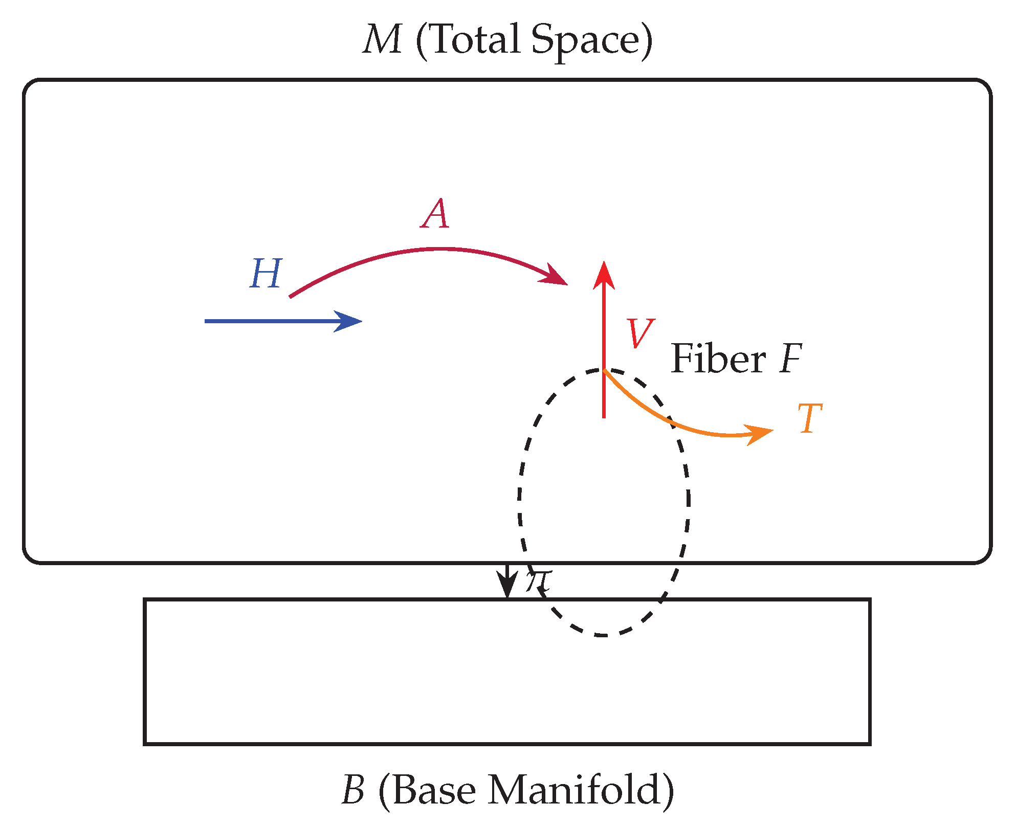
Figure 2.
Computational pipeline for curvature analysis in fibred Calabi–Yau manifolds. Starting from a Ricci–flat Kähler metric, one computes the Levi–Civita connection, projects onto horizontal and vertical distributions, evaluates the O’Neill tensors, and finally determines sectional curvature components.
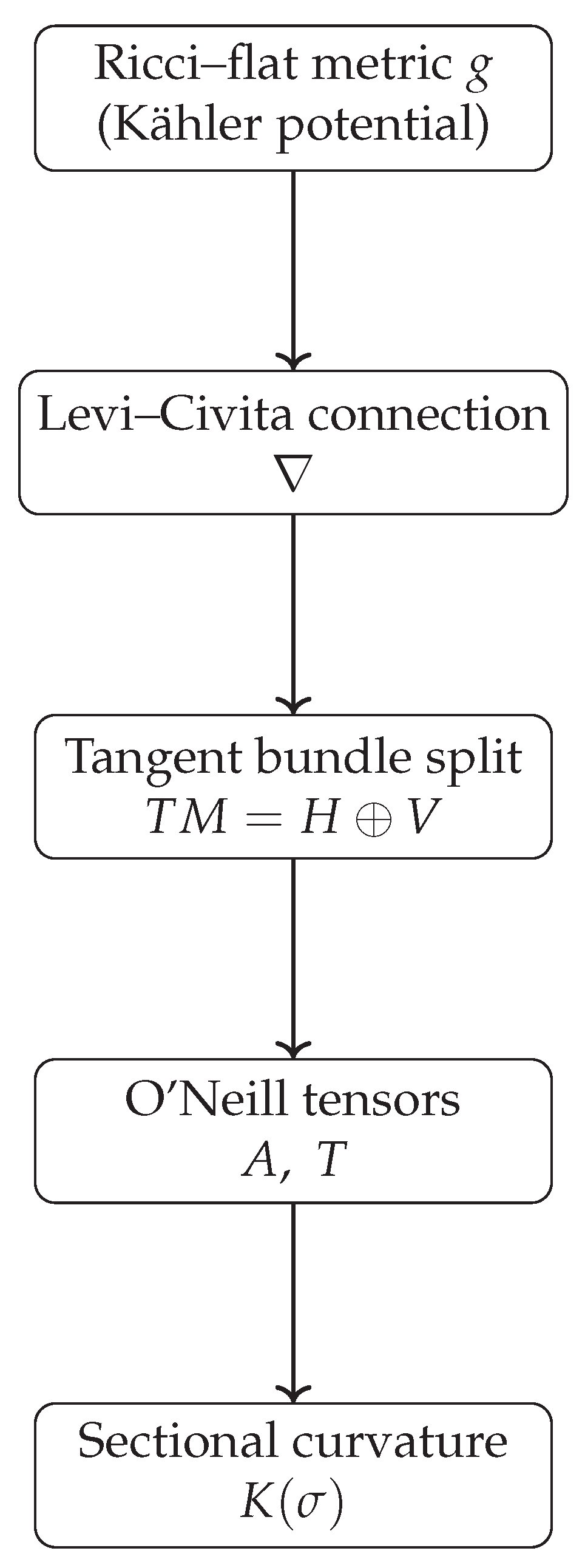

Table 1.
Decomposition of sectional curvature for a Riemannian submersion in terms of O’Neill tensors A and T.
Table 1.
Decomposition of sectional curvature for a Riemannian submersion in terms of O’Neill tensors A and T.
| Plane Type | Sectional Curvature Formula | Controlled By |
|---|---|---|
| Horizontal–Horizontal | Base + A | |
| Vertical–Vertical | Fiber + T | |
| Mixed (Horizontal–Vertical) | A–T interaction |
Table 2.
Qualitative behavior of O’Neill tensors and sectional curvature in different degeneration and collapse regimes for Calabi–Yau fibrations.
Table 2.
Qualitative behavior of O’Neill tensors and sectional curvature in different degeneration and collapse regimes for Calabi–Yau fibrations.
| Geometric Regime | Fiber Volume | Sectional Curvature Behavior | ||
|---|---|---|---|---|
| Product metric | constant | 0 | 0 | bounded; mixed curvature vanishes |
| Totally geodesic fibers | arbitrary | 0 | horizontal curvature modified by | |
| Semiflat collapsing limit | bounded | large | mixed curvature grows like | |
| Near singular fibers | curvature blow-up and anisotropy | |||
| Elliptic or torus fibration | constant or | bounded | 0 or large | vertical curvature induced extrinsically |
Disclaimer/Publisher’s Note: The statements, opinions and data contained in all publications are solely those of the individual author(s) and contributor(s) and not of MDPI and/or the editor(s). MDPI and/or the editor(s) disclaim responsibility for any injury to people or property resulting from any ideas, methods, instructions or products referred to in the content. |
© 2026 by the authors. Licensee MDPI, Basel, Switzerland. This article is an open access article distributed under the terms and conditions of the Creative Commons Attribution (CC BY) license (http://creativecommons.org/licenses/by/4.0/).
Copyright: This open access article is published under a Creative Commons CC BY 4.0 license, which permit the free download, distribution, and reuse, provided that the author and preprint are cited in any reuse.


