
Submitted:
31 January 2026
Posted:
03 February 2026
You are already at the latest version
Abstract
This paper analyzes the Binary Goldbach Conjecture (bGC) through a deterministic structural lens, employing a Failure Mode Analysis (FMA) framework to map prime and composite inventories onto the Left-Right Partition Table (LRPT). We establish structural identities governing the conservation of partition elements, demonstrating that the count of Prime-Prime (PP) pairs functions as a necessary deterministic residual. The analysis identifies tiered inadmissible failure states where, in each Tier, the exhaustion of composite inventories mathematically forces prime-prime partitions into existence to preserve information conservation. Numerical analysis for N up to 106 validates these findings, showing that the boundary of failure admissibility, parameterized by the ratio \( \hat{\lambda}_L(N) \), converges toward a global structural ceiling. Furthermore, by leveraging the midpoint symmetry of Goldbach primes, the FMA approach yields a ``Mirror Search'' mechanism for distal primes that demonstrates superior discovery efficiency compared to sequential scanning methods guided by the Prime Number Theorem. The analysis also reveals that the failure state (PP(N)=0) precipitates an information-theoretic paradox: it implies that the global prime counting function π(2N) can be fully reconstructed from the local modular geometry of a subset of composites, violating the established algorithmic irreducibility of the prime sequence.
Keywords:
arithmetic constraints
; Binary Goldbach Conjecture
; failure mode analysis
; factorial spectrum
; inadmissible state
; partition table
; prime symmetry
; structural identities
MSC: 11P32; 11N05; 11A41
1. Introduction
The Binary Goldbach Conjecture asserts that every even integer can be expressed as the sum of two primes. While the conjecture has been verified computationally for N up to [1], a structural proof remains elusive. Historically, analytic approaches such as the Circle Method and Sieve Theory have faced significant theoretical barriers, most notably the "Parity Problem," which limits the ability to distinguish between primes and products of two primes [2,3]. Furthermore, while probabilistic models like the Hardy-Littlewood heuristics [4] provide strong empirical evidence, they lack the deterministic necessity required to prove the non-existence of a failure state.
This work applies a Failure Mode Analysis (FMA) framework to the problem, investigating the structural conditions required for a “Failure State”, defined as a state where the count of prime partitions (or pairs) is zero, i.e., . By re-framing the conjecture as a resource allocation problem, we demonstrate that the existence of prime-prime pairs is not merely probable, but a deterministic consequence of inventory conservation.
The analysis focuses on the transition from the midpoint N to the partition space of . The fundamental data structure used is the Left-Right Partition Table (LRPT) [5], which maps the arithmetic inventory of primes and composites onto the row space of odd partitions. The framework demonstrates that the conservation of arithmetic inventory imposes strict lower bounds on , categorizing the problem into tiered inadmissible failure states. This research builds upon prior findings regarding additive pairings in the context of the bGC and, in particular, the structural implications of primes, coprimes and composites within such partitions [6,7,8].
The remainder of this paper is organized as follows: Section 2 establishes the foundational arithmetic definitions and partition classifications. Section 3 derives the Structural Identities that govern the conservation of elements within the LRPT. Section 4 presents the tiered Failure Mode Analysis, identifying the specific conditions under which a failure state becomes inadmissible. Section 5 analyzes the asymptotic behavior of the structural metrics, followed by numerical validation in Section 6. Finally, the Appendices discuss the efficiency of “Mirror Search” algorithms (Appendix A) and the information-theoretic implications of the failure state (Appendix B).
2. Definitions
This section establishes the foundational arithmetic parameters, partition classifications, and structural functions required to construct the Failure Mode Analysis (FMA) framework and the Left-Right Partition Table (LRPT).
2.1. Fundamental Parameters
Definition 1.
Let be an integer serving as the midpoint. An
odd partition
of is defined as a pair of odd integers such that:
The analysis is restricted strictly to odd integers.
Definition 2.
The total number of odd partition rows for a given N is denoted by :
This integer corresponds to the number of rows in the Left-Right Partition Table (LRPT) for the midpoint N.
Definition 3.
The
Top Right Entry (TRE)
is the largest integer in the partition space:
Definition 4.
The
Radius
of a partition represents its distance from the midpoint N:
Since x and y are odd integers with , the radius is always a non-negative integer.
Definition 5.
The
Minimum Distinct Radius, , is defined as the minimum radius among all distinct Prime-Prime (PP) partitions of :
where . Note that if N is prime, the partition is not considered since is not a distinct prime-prime partition.
Definition 6.
The
Maximum Radius, , is defined as the maximum radius among all Prime-Prime (PP) partitions of :
where .
2.2. Partition Classification
Definition 7.
Partitions are classified based on the primality of their components:
- PP: Prime-Prime (Goldbach pairs).
- PC: Prime-Composite.
- CP: Composite-Prime.
- CC: Composite-Composite.
The symbols , , , and denote the counts of these partitions in the LRPT for midpoint N.
2.3. Indicator Functions
Definition 8.
The following indicator functions define the state of the midpoint N:
2.4. Inventory and Arithmetic Functions
Definition 9.
The
Total Prime Inventory, , is the count of odd primes available in the partition interval:
Definition 10.
The prime factor counting functions are defined as:
- : The number of distinct odd prime factors of n.
- : The total number of odd prime factors of n (with multiplicity).
2.5. Composite Subsets
Definition 11.
The set of Composite-Composite partitions is decomposed into two disjoint sets based on the greatest common divisor (gcd) of the left component x and the midpoint N:
- Derived Composite Partitions ():
- Primitive Composite Partitions ():
Definition 12.
We define the complexity bounds for the Primitive Composites :
- The Theoretical Upper Bound, , is derived from the magnitude constraint :
- The Actual Maximum Complexity, , is the maximum number of distinct prime factors observed within the set:
It follows structurally that .
Definition 13.
The Primitive Composites set is partitioned into two disjoint subsets based on the complexity of the components relative to a parameter :
- Primitive Composite Partitions with Minimum Complexity ():
- Primitive Composite Partitions with Minimum Complexity ():
Structural Partition Identity:
2.6. Auxiliary Counts
Definition 14.
To support the Structural Identities, the following counts are defined:
- : Count of PP partitions excluding the midpoint .
- : Count of CC partitions excluding the midpoint .
- : Count of distinct odd composite integers in the LRPT.
- : Count of distinct odd prime integers in the LRPT.
2.7. Tiered FMA Criteria
Definition 15.
The tiered FMA criteria are defined as follows:
3. Structural Identities
The following identities govern the conservation of elements within the LRPT.
Partition Summation:
Distinct Element Counting:
Midpoint Decomposition:
Inventory Identities:
Structural Conservation:
Tiered Decompositions:
Remark 1.
The identities SI1 through SI9 establish the LRPT as a closed arithmetic system. The Structural Conservation Law (SI9) demonstrates that the count of prime pairs is not a probabilistic occurrence but a deterministic residual resulting from the subtraction of the composite inventory and the prime inventory from the total row space.
Remark 2.
Identity SI10 provides the critical separation between “Fixed” and “Free” arithmetic constraints. The Derived Composites are structurally forced by the existing prime factors of N (Tier II), whereas the Primitive Composites represent the intrinsic free space available to absorb the remaining arithmetic criterion (Tier III).
Remark 3.
The progression from SI11 to SI13 formalizes the sufficiency conditions for the Goldbach Conjecture. Proving is structurally equivalent to proving that the Active Primitive Composites are sufficient to fully saturate the arithmetic criterion . This forces the High-Complexity Remainder into a negative state (), necessitating the existence of prime pairs to balance the structural identity.
4. Structured Failure Mode Analysis
The Failure Mode Analysis (FMA) determines the conditions under which the failure state is mathematically impossible (inadmissible). From the Structural Identities derived in Section 3, a hierarchy of inadmissible failure states is defined, based on the balance between the arithmetic inventory (Supply) and the row space capacity (Demand).
4.1. Tier I—FMA: Prime Saturation
Tier I analyzes the arithmetic balance defined by the Structural Conservation Law (SI9). It represents a state of Arithmetic Saturation, where the prime inventory exceeds the composite inventory, and as a consequence some primes are structurally forced to form PP pairs.
Theorem 1.
For any midpoint N, if the first arithmetic deficit is negative, then the count of prime pairs must be strictly positive.
Proof.
The derivation begins with the Structural Conservation Law (SI9), which relates the partition counts to the arithmetic inventory:
By Definition 15, the Tier I deficit is defined as . Substituting this definition into SI
9 yields:
Rearranging the terms to compare the partition types:
If the arithmetic deficit is negative (), it strictly implies:
Since the count of composite pairs is non-negative (), the inequality necessitates that . □
This result shows how the analysis and findings discussed in Section 5.2 of [5] fit in the general and systemic FMA framework presented here.
4.2. Tier II—FMA: Structural Resistance
Tier I is sufficient for small N but fails as the density of primes decreases (). Tier II refines the analysis by accounting for Derived Composites (), which are composite pairs structurally forced by the prime factors of N. These pairs occupy row space but cannot contribute to .
Theorem 2.
For any midpoint N, if the second FMA criterion is negative, then .
Proof.
The proof employs the same saturation logic established in Tier I. We begin with the rearranged Structural Conservation Law:
Substituting the decomposition into the equation:
We isolate the relationship between the Primitive Composites and the prime pairs by subtracting from both sides:
By Definition 15, the right-hand side is exactly the Tier II criterion . If this value is negative (), the equation dictates:
Since the set of Primitive Composites is non-negative (), the strict inequality forces the existence of at least one prime pair (). □
Lemma 1
(Estimation Formula ). The Structural Resistance is approximated by the estimator function , which is derived using the Euler product formula over the odd domain:
Proof.
The derivation is based on the modular properties of the Left-Right Partition Table (LRPT). The total number of odd integer slots in the interval is represented by the scalar . The density of integers within this interval that share a common factor with N is calculated using the complement of the Euler product function. Let be the set of distinct odd prime factors of the midpoint. The proportion of integers coprime to N is given by . Consequently, the proportion of integers sharing a factor is determined as .
This density is applied to the interval size to estimate the total count of multiples. However, this set includes the prime factors themselves. Since results in a Prime-Composite (PC) pair (not a CC pair), these specific rows must be excluded. Thus, the count of distinct prime factors, , is subtracted from the total. □
Remark 4
(Numerical Validation of ). To assess the precision of the estimator relative to the exact Structural Resistance , a computational analysis was conducted over the interval . The absolute error was evaluated for each transition point. The results indicate that the approximation provides a highly accurate fit for the structurally enforced count. Across the entire domain of tested integers, the absolute error was found to be strictly bounded by . This empirical evidence confirms that serves as a reliable analytical predictor for the count of composite pairs enforced by the prime factors of the partition sum.
4.3. Tier III—FMA: Critical Threshold for Inadmissibility of Failure
The identification of the specific conditions required to render the failure state inadmissible is achieved by analyzing the saturation of the partition table row space. This is evaluated through the discrete count of active primitive composites, , which is subsequently modeled as a normalized ratio, .
Definition 16.
The Critical Active Count, , is defined as the maximum quantity of active primitive composites admissible in the partition table before a prime-prime solution is structurally forced:
When the active inventory reaches this threshold, the available capacity for composite-composite partitions is exhausted, forcing the formation of prime-prime pairs, in order to satisfy the structural conservation constraints of the LRPT table elements.
Definition 17
(Critical Complexity ). The Critical Complexity is defined as the minimum value required to satisfy the structural saturation condition established in Theorem 3. It identifies the specific complexity depth at which the cumulative active inventory exhausts the critical capacity :
The existence of a finite is sufficient to render the failure state structurally inadmissible.
Theorem 3.
For any midpoint N, the failure state is structurally inadmissible if the active primitive inventory at complexity k satisfies:
under the condition that if , the high-complexity reservoir must be strictly positive.
Proof.
Identity SI13 establishes the following relation:
Substitution of the definition for into (8) results in the expression:
In the case where , the right-hand side is strictly negative:
In the case where , the identity simplifies to:
The condition forces . In both scenarios, the failure hypothesis is contradicted by the arithmetic conservation of the partition table. □
To facilitate the analysis across varying magnitudes of N, a normalized metric is adopted. Such a transformation converts the above discrete analysis approach into a density threshold requirement relative to the total composite inventory.
We identify the critical threshold for the inadmissibility of a failure state () by analyzing the arithmetic gap between the composite inventory and the partition table capacity.
Definition 18
(Low Complexity Composite Ratio ). Let be the cardinality of the active odd composite inventory (partition rows) at iteration k. The active ratio is defined as the scalar relative to the total composite element inventory :
where .
Remark 5.
In the context of the Left-Right Partition Table (LRPT), the structural requirement to maintain a failure state (zero prime-prime pairs) dictates that each row must be occupied by at least one composite element. Since each row contains two distinct integer slots, the threshold for failure admissibility is defined by the saturation of the row space:
As , the numerical ratio approaches 1 as exhausts . However, the Goldbach solution is established as a deterministic necessity whenever , representing a state of over-saturation where the composite inventory exceeds the available row count, rendering a failure mode inadmissible.
Definition 19
(The Saturation Limit ). The structural limit ρ is defined as the ratio of the primitive capacity to the total composite inventory as :
Definition 20
(High Complexity Composite Ratio ). Let be the cardinality of the inactive odd composite inventory (partition rows) at iteration k. The inactive ratio is defined as:
where . As the complexity parameter k approaches its maximum value , the inactive reservoir is exhausted, satisfying the limit:
Remark 6
(Derivation of the Saturation Limit ). The structural limit ρ is derived by evaluating the active ratio at the maximum complexity state , where the high-complexity reservoir is exhausted ().
The definition of the ratio is:
From the Distinct Element Counting identity (SI2) and Midpoint Decomposition (SI4), the total composite inventory is:
Substituting the decomposition of composite pairs (since ) into the denominator yields the explicit saturation formula:
For midpoints with no odd prime factors (e.g., ), the derived composite count vanishes (). Since we cannot reasonably assume that , a scenario where is unrealistic. As , the primitive composite inventory dominates the prime-based counts, causing ρ to approach arbitrarily close from below ().
To identify the critical threshold for the inadmissibility of a failure state (), we utilize the identity derived from SI13:
Substituting the structural definition and the inventory identity into (SI9) yields:
Grouping terms by N and :
Definition 21
(Critical Active Threshold ). The critical active threshold is defined as the specific value of the active ratio that satisfies the zero-balance condition of the structural deficit equation. By setting the RHS of Equation (14) to zero and solving for , we obtain:
Structurally, this threshold represents the exact inventory density required to saturate the partition table’s remaining capacity after accounting for prime inventory and derived composite constraints. If the active ratio , the failure state becomes algebraically impossible.
These relationships are formally established in the following theorem.
Theorem 4
(Structural Inadmissibility of the Failure State). For any even integer , the failure state is structurally inadmissible whenever the active ratio strictly exceeds the critical threshold:
Under this condition, the structural deficit becomes strictly negative, which algebraically forces the existence of Prime-Prime pairs () to satisfy the partition conservation laws, even in the limiting case where the inactive reservoir is exhausted ().
Proof.
We analyze the structural identity derived in Equation (14):
By Definition 21, the critical threshold is the root where the Right-Hand Side (RHS) equals zero. We observe that the RHS is strictly decreasing with respect to , as the derivative is dominated by the term . Consequently, applying the condition renders the RHS strictly negative:
Rearranging the inequality yields:
Since the inactive inventory is non-negative (), strictly positive solutions for prime pairs are structurally forced:
This completes the proof. □
Remark 7
(Scaling Dominance of Prime Inventory). It is important to note that the derived composite constraint does not threaten the strict negativity of the structural deficit. The term scales based on the distinct prime factors of N (specifically, ), which grows extremely slowly (e.g., ). In contrast, the prime inventory term scales asymptotically as . Consequently, for all large N, the magnitude of the prime inventory deficit dominates the modular constraints:
Remark 8
(Global Ceiling vs. Operational Threshold). A critical distinction exists between the global structural ceiling and the local operational threshold. The condition:
represents the absolute saturation point where the row space is exhausted regardless of prime inventory magnitude. As shown, this limit is practically unreachable. However, for finite midpoints, the state of forced inadmissibility is governed by the critical active threshold. By omitting negligible lower-order terms (), we obtain the operational approximation:
Due to the presence of , this value is strictly lower than the asymptotic limit of . Consequently, the condition for inadmissibility is satisfied at lower composite densities, rendering the failure state inadmissible before the global capacity limit is reached.
This is used to define a conservative boundary estimate for in Section 4.3.1 and is tested numerically in Section 6.
Remark 9
(Necessity of Positive Capacity). The failure state requires the Right-Hand Side (RHS) of Equation (14) to be non-negative. Because the prime inventory term imposes a strictly negative load for all , the structural capacity term must strictly exceed this deficit to sustain the failure state. This implies that structural admissibility becomes infeasible well before the ratio reaches . As , increases and crosses the operational threshold , rendering the failure state structurally inadmissible.
4.3.1. The Conservative Failure Boundary
A conservative boundary for failure inadmissibility is established. We utilize the critical active threshold defined in Definition 21. To obtain a universal sufficiency condition that depends solely on the prime inventory, we define the estimator by imposing the “blank slate” condition, setting the derived composite term to zero in Equation (15).
Definition 22
(Conservative Boundary Estimator). The Conservative Boundary Estimator is defined as the upper bound of the critical active threshold :
Structurally, since and it follows that . Therefore, satisfying the condition guarantees structural inadmissibility for all midpoints N, regardless of their specific prime factors.
Definition 23
(Structural Safety Margin). The margin is defined as the normalized difference between the global structural ceiling of and the conservative boundary :
The progression of the critical threshold is governed by the asymptotic density of the prime inventory. As N increases, the scaling of follows the Prime Number Theorem (). In the limit , the ratio approaches zero. Substitution of this limit into the estimator demonstrates monotonic convergence toward the global structural ceiling:
This convergence establishes that the structural requirement for the inadmissibility of a failure state remains bounded by a global constant. While the "occupancy pressure" in the LRPT table from the prime inventory is most dominant at small N, the system remains structurally constrained at large N because the required active composite ratio never exceeds the theoretical ceiling of . This trend confirms that even under the conservative assumption of zero derived structural assistance (), the required ratio for saturation remains strictly bounded. The numerical evolution of is presented in Section 6.
4.4. Continuous Radical Complexity Model
The structural models previously discussed rely on the partitioning of the primitive composite inventory into a discrete sequence of nested subsets, defined by the prime factor count of the partition summands. To resolve the granularity limitations of this discrete approach, which segments the inventory into discontinuous tiers, a continuous model based on the Radical Complexity Gradient is introduced, to analyze the active inventory without discrete partitioning. For any partition , the radical complexity is defined as the logarithmic mapping of the square-free product normalized by the midpoint:
where . This maps the primitive composite inventory to the spectrum , since the product of partition components satisfies .
Definition 24
(Continuous Active Inventory). The continuous active inventory is defined as the subset of primitive composites satisfying the complexity bound γ:
The cardinality is a monotonically non-decreasing step function with respect to γ.
Example 1.
Consider a partition for where and . The absolute product is . The radical is . The complexity is:
This value places the partition in the active inventory for all , despite the magnitude of exceeding N.
To identify the saturation threshold, we define the Critical Radical Density as the infimum of the complexity parameter required to satisfy the structural deficit .
Definition 25
(Critical Radical Density).
At this critical value, the structural identities (SI4) and (SI13) imply:
Since is strictly determined by the complement , the existence of implies . If is strictly less than the maximum complexity of the set, the inequality structurally forces .
4.5. Evolution of and for
The following table shows the values of the conservative boundary estimator and the critical radical density across a logarithmic progression of values for N.
The empirical values in Table 1 substantiate the theoretical derivation of the conservative boundary. The observed monotonic convergence of toward confirms that the structural saturation requirement remains strictly bounded below the global ceiling. Furthermore, the non-vanishing safety margin provides numerical evidence that the partition space never reaches the theoretical limit required to permit a failure state. Additionally, the data indicates a monotonic decrease in as N increases, consistent with the asymptotic behavior of the active composite ratio .
5. Asymptotic Trends of Key FMA Metrics
We analyze the asymptotic behavior of three structural FMA metrics as : the growth rate of the critical complexity index , the decay rate of the normalized ratios , and the convergence of the normalized ratio . These derivations serve as a theoretical baseline for the numerical analysis in Section 6, where the empirical trajectories of , , and are benchmarked against their predicted asymptotic trends to validate the FMA structural convergence findings.
5.1. Estimation of Asymptotic Growth Rate of as
The structural analysis in Section 4.3.1 established that the critical active threshold converges asymptotically to . This convergence implies that to guarantee the inadmissibility of a failure state, the active inventory must capture approximately half of the total composite population. Consequently, the critical complexity represents the median number of distinct prime factors for integers in the interval .
We invoke the Hardy-Ramanujan Theorem [9], which establishes that the normal order of the number of distinct prime factors for an integer n is . Furthermore, the Erdos-Kac Theorem [10] proves that the distribution of is asymptotically Gaussian with mean and variance .
For a Gaussian distribution, the median and the mean are asymptotically equivalent. Therefore, the complexity index k required to accumulate the first of the composite inventory scales directly with the normal order:
This scaling law provides the theoretical justification for the stability observed in the numerical data. In contrast, the theoretical upper bound for complexity derived from magnitude constraints is . Since for all large N, this confirms the existence of a substantial combinatorial safety margin, as the system reaches a state of forced inadmissibility using only a negligible fraction of the theoretically available complexity depth.
5.2. Asymptotic Decay of as
The normalized Minimum Distinct Radius, defined as , indicates the proximity of the first prime-prime partition to the midpoint N. The scaling behavior is derived by treating the primality of components x and y as independent events, consistent with the Hardy-Littlewood k-tuple conjecture [4].
According to the Prime Number Theorem, the local density of primes near N is approximately . The probability that a given partition row constitutes a prime-prime pair is modeled as:
Assuming a geometric distribution for the distance to the first success in the row space, the expected number of trials—and thus the expected radius—scales as the inverse of the probability:
Normalizing by the midpoint yields the asymptotic decay rate:
5.3. Asymptotic Convergence of as
The normalized Maximum Radius, , is determined by the magnitude of the smallest prime in the partition set . Unlike the MDR, which requires simultaneous primality of variable components , the determination of fixes the left component to the sequence of small primes and tests the primality of the complement .
Assuming the events are independent, the probability that the complement is prime is given by the density near :
The expected number of trials k required to observe the first valid partition follows a geometric distribution with expectation . To find the magnitude of the smallest component , we approximate the k-th prime using the asymptotic law :
Substituting this expectation into the radius definition yields the asymptotic expression for the normalized maximum radius:
This derivation confirms that the ratio converges to unity from below, with the “gap” from the edge scaling almost linearly with , modulated by a polylogarithmic factor.
6. Numerical Analysis
The objective of this analysis is the empirical validation of the findings discussed in the previous sections. The FMA approach, in conjunction with the LRPT table, its associated metrics, and conservation laws, constitutes a comprehensive systemic testbed for the analysis and testing of hypotheses related to the Binary Goldbach conjecture, or any other arithmetic system with similar structure, columnar-type symmetry, and conservation laws.
The analysis of the structural characteristics of the odd partitions of for was implemented using the Google Colab multi-core Python programming and execution environment. To efficiently manage long processing times, large data output volumes, and risks related to runtime timeouts, the coding architecture incorporated three primary safeguards: batched implementation, persistent storage, and seamless resumption in case of mid-run interruptions. With these measures in place, and with the code optimized for a multi-core environment, the total execution time was approximately 3–4 days.
Data processing and graphing utilized three statistical techniques: (1) moving averages to smooth high-frequency fluctuations over large intervals of N; (2) data binning to compress datasets for visualization without information loss; and (3) computational functions for indexing and categorization. These techniques are discussed in greater detail in the subsequent sections as they apply to each FMA measure.
6.1. and as
The numerical evolution of and for follows the theoretical predictions established in Section 4.3 and Section 5.1, as illustrated in Figure 1. The dashed line (left axis) denotes the asymptotic approximation of as from Equation (26), scaled by a factor of with an offset of to optimize the fit for .
The graph also displays the average (orange line, left axis), calculated using a 50-row binning window that reduces the dataset from to points. The persistent high-frequency fluctuations observed in the larger values of are characteristic of the variability in the structural tension required to balance the primitive composite inventory across different N. Further analysis is required to link to the characteristics of the Factorial Spectrum of N—specifically the number, multiplicity, relative size, and variance of its prime factors. This future research direction necessitates a deeper statistical analysis of partition data alongside the factorization characteristics of N. Such analysis could provide insights into the underlying causes of the varying tension required to satisfy , beyond the magnitude of N itself.
The solid line represents (blue line, right axis) as defined in Equation (1). It demonstrates a margin of approximately 3–4 times between and ; specifically, for larger N. This implies that the required balancing of the primitive composite inventory is consistently achieved at a numerical complexity level significantly lower than the theoretical worst-case bound.
6.2. and as
The ratios of and are plotted after performing a 50-row binning and calculating the average value for each bin. Each ratio converges numerically and asymptotically to the values predicted from the analysis in Section 5.2 and Section 5.3.
Figure 2 illustrates the convergence of to 0 and Figure 3 illustrates the convergence of to 1 as N increases. This trend indicates a persistent structural pattern where at least one symmetric Prime-Prime partition exists in the vicinity of the midpoint N (small radius) and the endpoint (large radius). Consequently, an optimized Mirror Search strategy for primes in is most efficient when concentrated around these two loci. This optimization is analyzed in Appendix A.
Furthermore, the data demonstrates that for larger N, substantiating the existence of distinct PP partitions in the lower half of the LRPT (closer to the midpoint). In this context, the case of , where the sole distinct PP partition resides in the upper half of the table, appears to be a unique anomaly. Conversely, the trajectory suggests a persistent pattern regarding the existence of at least one PP partition in the upper half of the LRPT.
The dashed line in Figure 2 represents the asymptotic approximation of as , derived in Equation (27). A scalar factor of was applied to optimize the fit to the observed data for .
Similarly, the ratio is plotted in Figure 3. The dashed line represents the asymptotic approximation of as , derived in Equation (28), with a scalar factor of applied to optimize the fit for .
6.3. and as
Figure 4 displays the evolution of and for , computed using a 50-row binning average. The solid and dashed lines represent the observed active ratio and the conservative boundary estimator defined in Equation (19), respectively.
The observed value of corresponds to the minimum complexity k required to satisfy the condition , which implies . The graph demonstrates that for large N, this value is approximately lower than the limit imposed by the conservative boundary estimator for that N.
The high-frequency fluctuations observed in the graph of for larger values of N indicate that the observed ratio of primitive composite partitions to the total composite inventory exhibits slight volatility while maintaining a consistent upward trend as N increases.
6.4. Tier III Criteria as
In the preceding sections, we established the operational ranges for the three-tiered FMA framework. Prime saturation (Tier I) guarantees for , consistent with prior research [5], while Tier II extends this guarantee to . A specific tier validates the condition if its corresponding criterion is strictly negative: (Tier I), (Tier II), or (Tier III).
To accommodate the varying operational ranges of the tiers, the binning window was reduced to 25 rows. Prior to binning, a 100-row moving average was applied to mitigate high-frequency fluctuations that would otherwise obscure the visual trends. As observed in Figure 5, these fluctuations are visibly more persistent for Tier III ().
Figure 5 illustrates how each subsequent tier extends the domain of admissibility as N increases, quantifying the structural dynamics required to maintain as .
The graph demonstrates that the effective domain of each earlier tier diminishes as N increases, justifying the necessity of the Tier III analysis parameterized by k, , or . For the range , the complexity level is sufficient to maintain for all points, thereby guaranteeing .
Notably, the observed necessary complexity is significantly lower than the theoretical maximum derived in Definition 12.
7. Conclusions
This research has presented a structural investigation of the Binary Goldbach Conjecture through the lens of Failure Mode Analysis (FMA). By mapping the arithmetic inventory of primes and composites onto the fixed geometry of the Left-Right Partition Table (LRPT), we have established a framework that treats the existence of Prime-Prime () partitions not as a probabilistic occurrence, but as a deterministic consequence of information conservation.
The central finding of this work is the identification and tiered manifestation of the Structural Conservation Law, which dictates that the count of prime-prime pairs operates as a deterministic arithmetic residual. The analysis demonstrated that for a “Failure State” () to exist, the inventory of composite numbers would need to saturate the partition row space to a critical density (). This saturation effectively deprives the prime inventory of the composite partners required for pairing, thereby forcing prime-prime partitions into existence.
Additional insights derived from this framework include:
- Tiered Inadmissibility: The FMA approach categorizes the conditions for failure into three hierarchical tiers. Tier I (Prime Saturation) precludes failure for small N where prime density exceeds composite capacity. Tier II (Structural Resistance) extends this domain by identifying the Derived Composite Inventory (), which is structurally forced by the prime factors of the midpoint. Finally, Tier III (Critical Complexity) establishes the general sufficiency condition for large N, identifying the critical complexity depth at which the Active Primitive Composite Inventory () saturates the remaining row space, rendering the failure state structurally inadmissible.
- Asymptotic Stability: The derivation of the critical complexity relative to the theoretical upper bound confirms that the partition system becomes increasingly stable. The analysis indicates that the partition space is saturated by low-complexity composites () long before the theoretical complexity limit is reached, creating an expanding combinatorial safety margin as N increases.
- Deterministic vs. Probabilistic: Unlike heuristic models that rely on the pseudorandom distribution of primes, the FMA framework relies on the rigid modular constraints of composite pairings. The resulting Structural Identities imply that the global prime counting function is inextricably linked to the local geometry of partitions, suggesting that a failure of the conjecture would necessitate a violation of the algorithmic irreducibility of the prime sequence.
In summary, this work moves beyond existence-based searching to define the boundaries of Structural Inadmissibility. While not replacing traditional analytic methods, the FMA framework offers a novel, deterministic perspective: that the Binary Goldbach Conjecture is likely true not because the primes are random enough to hit a target, but because the composites are structurally constrained from blocking all possible solutions.
Appendix A. Mirror-Prime Search Analysis
This appendix evaluates the search efficiency implications of the FMA framework under the assumption of standard probabilistic prime distribution models. Specifically, we define the search problem as identifying a prime given the known inventory of primes . Unlike the deterministic structural proofs presented in the main body, these results rely on the Prime Number Theorem (PNT) and the Hardy-Littlewood k-tuple conjecture.
Appendix A.1. Search Definitions
Definition A1.
Let T represent the number of primality tests performed and represent the distance from the search origin N to the discovered prime q. TheSearch Leverage is defined as:
Definition A2.
TheSearch Efficiencyη is defined as the inverse of the computational cost required to identify a prime :
A higher η indicates a lower computational cost per discovery.
Theorem A1.
Under the assumption of the Prime Number Theorem and the Hardy-Littlewood model, the leverage of a sequential search scales as , while the leverage of the FMA mirror search scales as .
Proof.
For a sequential search starting at N, the Prime Number Theorem implies the expected distance to the next prime is . Since every candidate must be tested, the number of trials T is proportional to the gap, yielding . Substitution into Equation (A1) yields .
For the FMA method searching for a symmetric Prime-Prime partition , the search variable is the radius R. Under the Hardy-Littlewood model, the expected radius for the first occurrence (MDR) scales as . However, due to the filtering of composite candidates via modular constraints, the effective number of trials T required to traverse this radius is proportional to the prime density, . Substitution yields:
□
Appendix A.2. Local Prime Search Analysis
The objective of the local search is to identify the immediate next prime , thereby minimizing the distance . To maximize local probability, the FMA framework employs a descending prime anchor protocol, utilizing the largest known primes to first check those mirrors located closer to N.
Lemma A1.
In a local window , the expectation of search efficiency for the PNT strategy is greater than or equal to that of the FMA strategy.
Proof.
Let represent the local window length. The sequential PNT strategy evaluates all odd integers (candidate density ). The FMA strategy evaluates a restricted set of symmetric pairs determined by modular constraints. In a local window where primes are dense, the PNT strategy’s exhaustive scan minimizes the risk of skipping a prime, thereby minimizing the expected number of trials required for the first success. Since , it follows that . □
Example A1.
To illustrate the efficiency gap in local search, consider the midpoint . We seek the first prime .
-
PNT Strategy (Sequential Scan):The search checks odd integers .
- 1.
- Test 4013: Prime .
Result: Success in . Efficiency . -
FMA Strategy (Descending Anchors):The search checks mirrors of known primes in descending order ().
- 1.
- Anchor : Test (Div 5). Fail .
- 2.
- Anchor : Test . Prime . Success .
Result: Success in partition checks. Efficiency .
In this local context, the PNT strategy is more efficient for identifying the immediate next prime.
Appendix A.3. Distal Prime Search Analysis
The objective of the distal search is to identify a deep prime near the upper boundary , thereby maximizing the discovery distance .
Recalling Definition 6, the Maximum Distinct Radius, , determines the maximum discovery distance to a prime . This distance is maximized at the boundary , corresponding to the smallest prime anchor . To maximize search leverage, the FMA protocol starts by testing mirrors of small known prime anchors that resolve to primes located closer to the upper boundary.
Lemma A2.
Testing candidates of the form for known primes identifies a prime with a maximum trial budget . This achieves a distal discovery leverage that exceeds a sequential Bertrand search by a factor of .
Proof.
Consider the search for a prime q at the upper boundary of the Bertrand interval (). (1) Under sequential scanning, the number of trials required to reach the boundary is proportional to the distance . (2) Under FMA, the mirror of is the Top Right Entry (TRE), . Testing distal mirrors utilizes the known density of primes as anchors. (3) The trial budget for a complete FMA search corresponds to the prime inventory . (4) The search leverage is defined as . For the distal mirror ():
In contrast, the leverage for sequential discovery near the boundary is . □
Example A2.
To illustrate the leverage divergence in distal discovery, consider the midpoint (). We compare the effort required to identify the boundary prime ( pair with ).
Sequential Strategy (Reverse Linear Scan):The search scans odd integers downwards from the upper boundary .
- Test 799 ():Fail(Composite).
- Test 797: Prime .
Result: Prime discovered in trials.
Mirror Strategy (FMA Edge-In):The search tests mirrors of known small prime anchors in ascending order to resolve .
- Anchor : Test Mirror . Prime .
Result: Prime discovered in trial.
The FMA strategy identifies the distal prime immediately by leveraging the known primality of the anchor . In contrast, the linear scan must evaluate the intermediate composite candidate 799. This demonstrates how the FMA framework utilizes the modular geometry of the partition table to structurally filter non-viable candidates at the interval boundaries.
Conclusion: The Goldbach Accelerator
The comparative analysis of search mechanics indicates that the Goldbach symmetry functions as a framework for computational efficiency. Specifically, the midpoint symmetry allows for a structured exploration of the prime field that exceeds the distal reach of linear search methods under fixed-budget constraints. This identifies the Goldbach symmetry as an algorithmic accelerator, mapping the density of the known prime field onto the distal interval with superior leverage compared to sequential scanning.
Furthermore, the efficiency of these dual search protocols may be enhanced by analyzing the sensitivity of and to the arithmetic characteristics of N, such as the number, variance, and multiplicity of its prime factors, enabling adaptive calibration and optimization of the search anchors. This is an area of future research.
Appendix B. Implications of Failure State (PP=0) on Prime Counting
In this section, we demonstrate that the assumption permits the calculation of the global prime inventory using a conditional testing algorithm that queries strictly fewer integers than the total population of the interval. Crucially, this relative reduction persists even when standard composite pre-filtering (e.g., excluding multiples of 3 or 5) is applied symmetrically to the domain. Drawing on the fundamental dichotomy between arithmetic structure and pseudorandomness established by Tao [11], and the algorithmic irreducibility of prime sequences described by Chaitin [12], we demonstrate that this precipitates an information-theoretic contradiction. The failure state implies that the global prime counting function can be fully reconstructed from the local modular geometry of a subset of composites, violating the established algorithmic irreducibility of the prime sequence.
Appendix B.1. The Conditional Testing Algorithm
Consider an algorithm designed to identify the set of odd Composite-Composite pairs, , for a given non-prime integer N. The algorithm iterates through the partition rows , corresponding to the odd partition pairs such that and .
The testing protocol is conditional:
- 1.
- LHS Test: Perform a primality test on the left-hand summand x.
- 2.
- Condition A (Prime): If x is prime, terminate the process for this row. (Under the hypothesis , a row with a prime x cannot be a pair, so the status of y is irrelevant for determining ).
- 3.
- Condition B (Composite): If x is composite, proceed to test the right-hand summand y.
- 4.
- Classification: If both x and y are confirmed composite, increment the count .
Appendix B.2. Derivation of Computational Counts
We now quantify the information cost of this algorithm compared to the baseline requirement for determining the Total Prime Inventory () of the unique integers in the interval.
Let be the set of all unique odd integers in the interval . We introduce the parity indicator function , which equals 1 if N is odd and 0 otherwise. This accounts for the center partition where the left and right summands map to the same unique integer.
The cardinality of the unique set is:
Next, we calculate , the number of unique primality tests performed by the Conditional Algorithm:
- LHS Tests: We test every unique x in the left column. Count .
- RHS Tests: We test y if and only if x is composite. However, if N is odd, the center element has already been tested as (since N must be composite under the failure hypothesis). Therefore, we subtract the center case to avoid double-counting.
The count of unique RHS tests is the number of LHS composites minus the shared center case:
The total number of tests performed is:
Appendix B.3. The Invariant Information Deficit
Subtracting the actual tests from the total population reveals the Information Deficit :
This confirms that regardless of whether N is even or odd, the assumption allows the global state to be determined while skipping exactly independent checks. The ability to determine the exact global inventory of primes while systematically bypassing independent checks constitutes a violation of Information Conservation. This contradicts the established property that the prime sequence possesses irreducible pseudorandomness [11,12], implying that the existence of Goldbach partitions () serves as the structural residual required to preserve the algorithmic incompressibility of the prime sequence relative to local modular constraints.
Corollary A1
(Extension to Prime Midpoints). The above information-theoretic contradiction extends to the case where the midpoint N is prime. If we assume that (representing only the identity partition ), the conditional logic of the testing algorithm remains valid for all off-center rows. Specifically, for every prime , the assumption forces the complementary y to be composite. This allows the precise determination of the global prime inventory while skipping independent checks. To resolve this paradox and restore algorithmic irreducibility, the partition space must contain at least one distinct prime-prime pair, implying for all prime .
References
- Oliveira e Silva, T.; Herzog, S.; Pardi, S. Empirical verification of the even Goldbach conjecture and computation of prime gaps up to 4·1018. Math. Comp. 2014, 83, 2033–2060. [Google Scholar] [CrossRef]
- Nathanson, M.B. Additive Number Theory: The Classical Bases. In Graduate Texts in Mathematics; Springer-Verlag: New York, NY, USA, 1996; Volume 164. [Google Scholar]
- Selberg, A. Elementary Methods in the Theory of Primes. Norske Vid. Selsk. Forh., Trondheim 1947, 19, 64–67. [Google Scholar]
- Hardy, G.H.; Littlewood, J.E. Some problems of ’Partitio numerorum’; III: On the expression of a number as a sum of primes. Acta Mathematica 44, 1–70, 1923. [CrossRef]
- Papadakis, I. On the Binary Goldbach Conjecture: Analysis and Alternate Formulations Using Projection, Optimization, Hybrid Factorization, Prime Symmetry and Analytic Approximation. Math. Comput. Sci. 2024, 9, 96–113. [Google Scholar] [CrossRef]
- Papadakis, I.N.M. On the Universal Encoding Optimality of Primes. Mathematics 2021, 9, 3155. [Google Scholar] [CrossRef]
- Papadakis, I.N.M. Algebraic Representation of Primes by Hybrid Factorization. Math. Comput. Sci. 2024, 9, 12–25. [Google Scholar] [CrossRef]
- Papadakis, I. Representation and Generation of Prime and Coprime Numbers by Using Structured Algebraic Sums. Math. Comput. Sci. 2024, 9, 57–63. [Google Scholar] [CrossRef]
- Hardy, G.H.; Ramanujan, S. The normal number of prime factors of a number n. Quart. J. Math. 1917, 48, 76–92. [Google Scholar]
- Erdos, P.; Kac, M. The Gaussian law of errors in the theory of additive number theoretic functions. Am. J. Math. 1940, 62, 738–742. [Google Scholar] [CrossRef]
- Tao, T. Structure and Randomness in the Prime Numbers. In An Invitation to Mathematics; Schleicher, D., Lackmann, M., Eds.; Springer: Berlin/Heidelberg, Germany, 2011; pp. 1–7. [Google Scholar]
- Chaitin, G.J. Algorithmic Information Theory; Cambridge University Press: Cambridge, UK, 1987. [Google Scholar]
Figure 1.
(orange line, left axis), (dashed line, left axis), and (solid line, right axis) as .
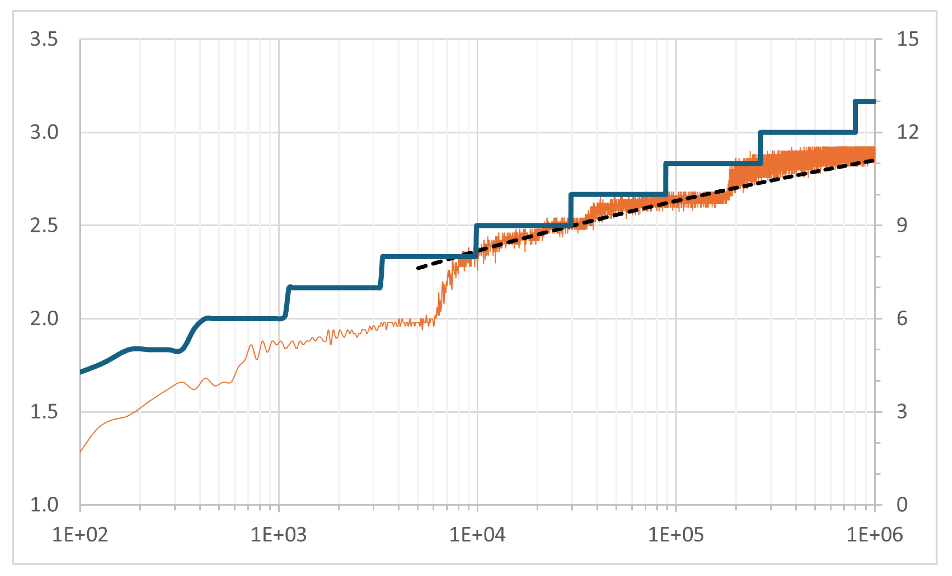
Figure 2.
(solid line) and (dashed line) as .
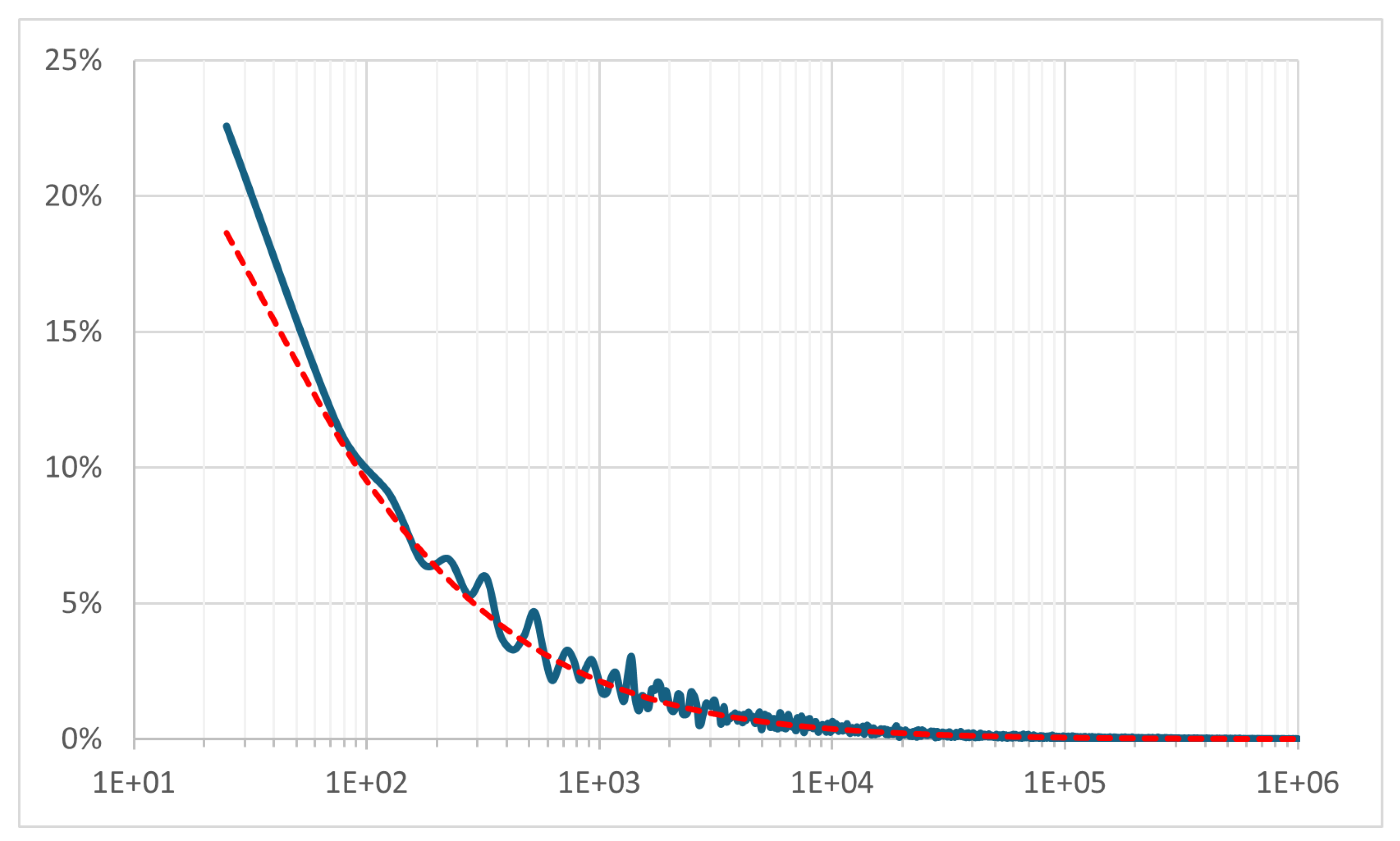
Figure 3.
(solid line) and (dashed line) as .
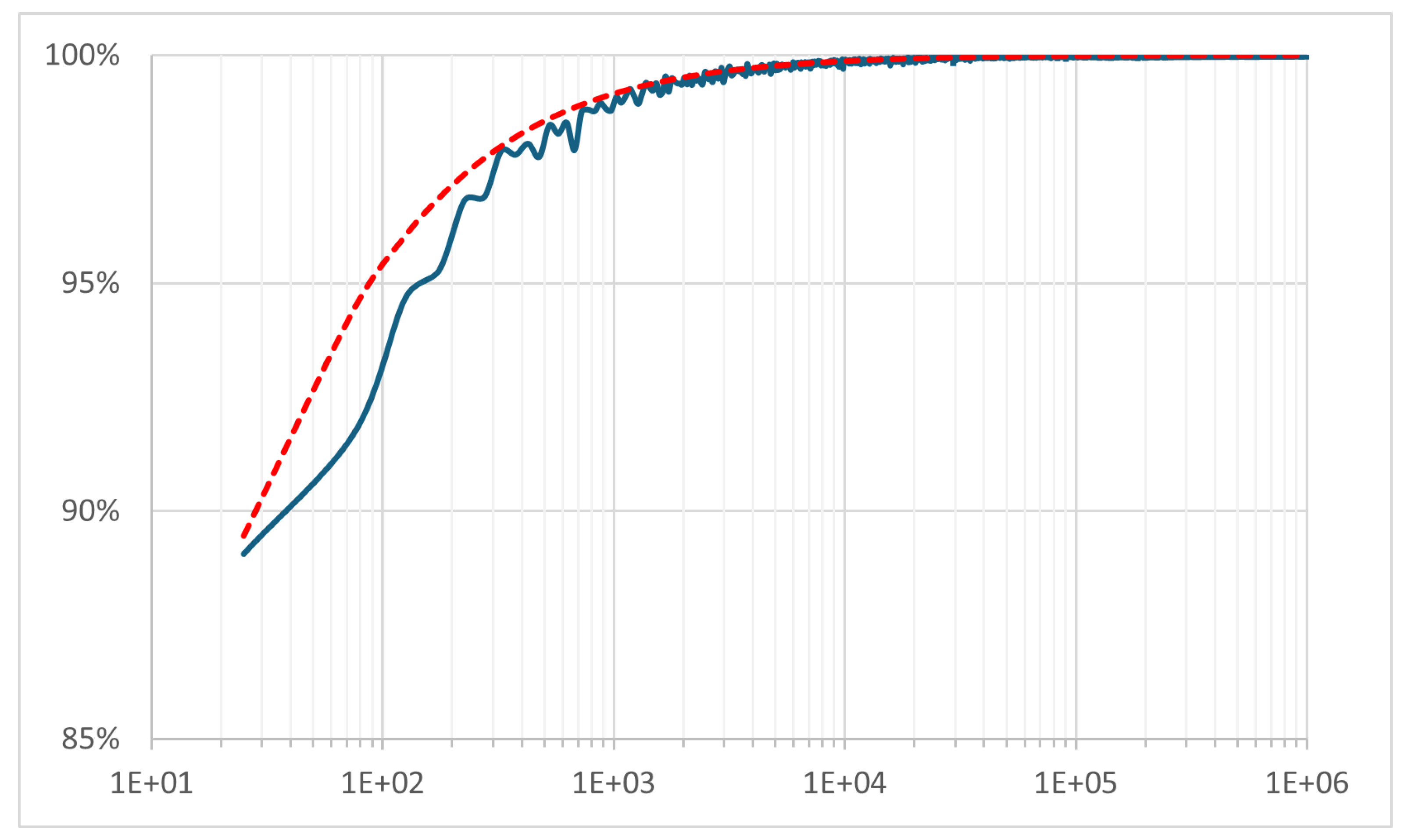
Figure 4.
and as .
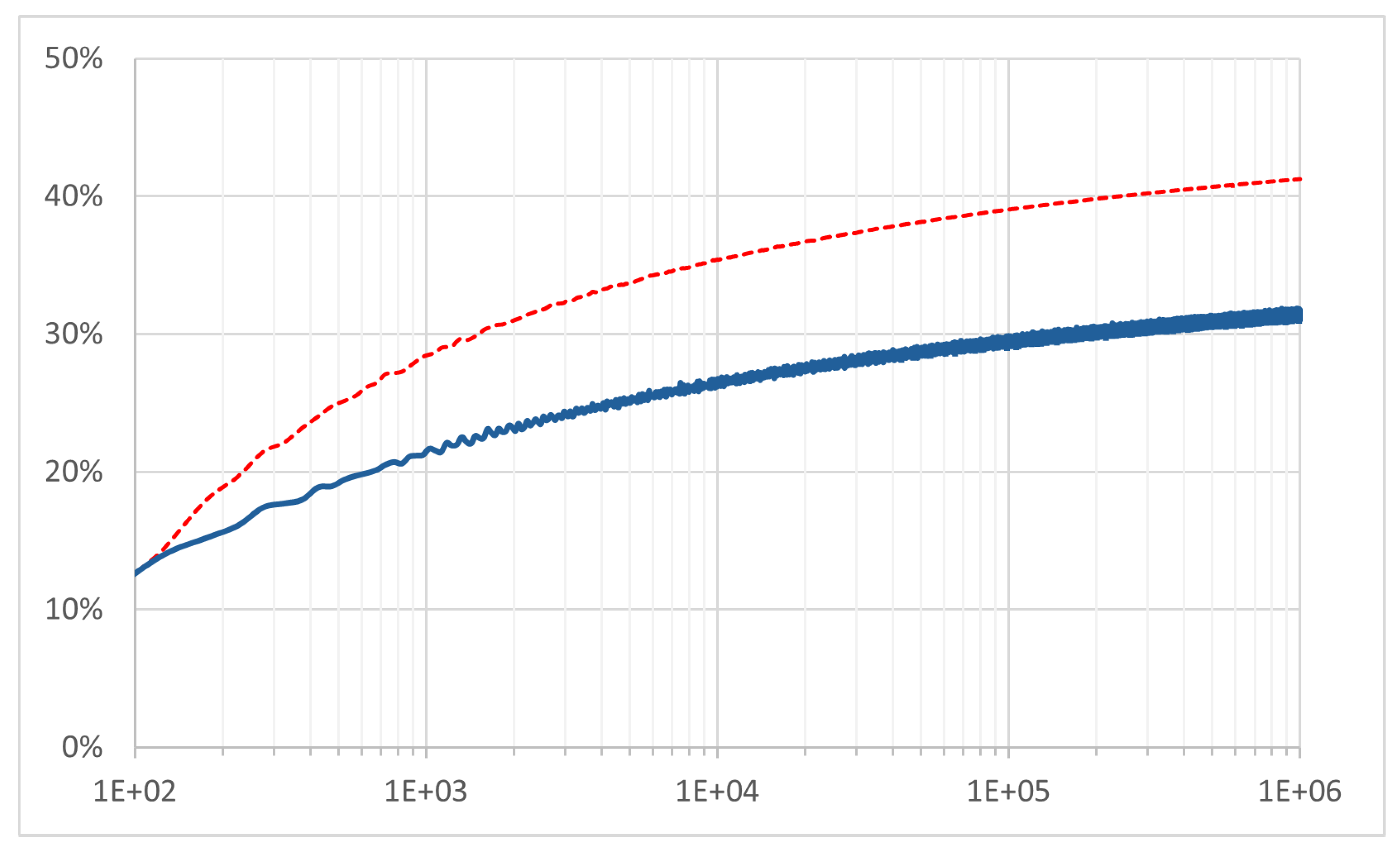
Figure 5.
FMA RHS criteria for Tier I (green), Tier II (purple) and Tier III: (orange); (blue); (red, dashed) as .
Figure 5.
FMA RHS criteria for Tier I (green), Tier II (purple) and Tier III: (orange); (blue); (red, dashed) as .
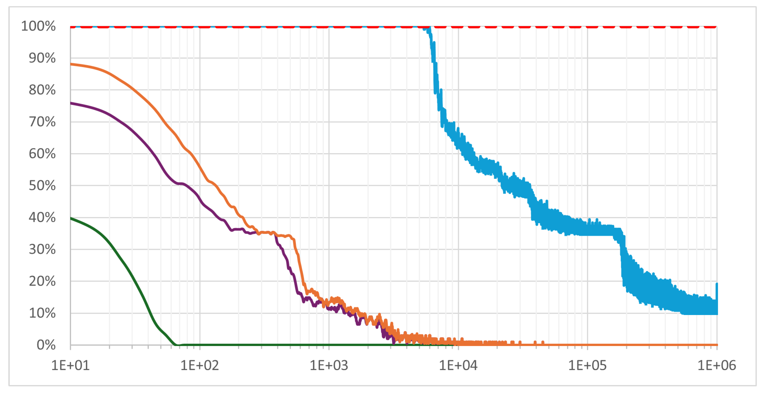

Table 1.
Evolution of Conservative Boundary , Safety Margin , and Critical Radical Density for ().
| m | N | (%) | ||
|---|---|---|---|---|
| 2 | 0.107 | 78.6 | 2.00 | |
| 3 | 0.285 | 43.1 | 1.99 | |
| 4 | 0.354 | 29.2 | 1.92 | |
| 5 | 0.390 | 21.9 | 1.85 | |
| 6 | 0.413 | 17.5 | 1.78 | |
| 7 | 0.427 | 14.6 | 1.71 | |
| 8 | 0.438 | 12.5 | 1.64 | |
| 9 | 0.446 | 10.9 | 1.58 | |
| 10 | 0.452 | 9.7 | 1.52 |
Disclaimer/Publisher’s Note: The statements, opinions and data contained in all publications are solely those of the individual author(s) and contributor(s) and not of MDPI and/or the editor(s). MDPI and/or the editor(s) disclaim responsibility for any injury to people or property resulting from any ideas, methods, instructions or products referred to in the content. |
© 2026 by the author. Licensee MDPI, Basel, Switzerland. This article is an open access article distributed under the terms and conditions of the Creative Commons Attribution (CC BY) license.
Copyright: This open access article is published under a Creative Commons CC BY 4.0 license, which permit the free download, distribution, and reuse, provided that the author and preprint are cited in any reuse.


