Submitted:
30 January 2026
Posted:
02 February 2026
You are already at the latest version
Abstract
Fast-curing polyurethane (PU) systems are attractive for high throughput manufacturing, but quantifying cure kinetics, gelation, and cure-dependent glass transition temperature (Tg) is difficult, especially at low degree of cure (DoC). Here, a fast-reacting BASF PU formulation was studied using non-isothermal differential scanning calorimetry (DSC) at multiple heating rates, rheometry at 50 °C, and molecular dynamics (MD) simulations to extend Tg(α) in the low-DoC regime. DSC provided reaction enthalpy and conversion histories, and Kamal–Sourour (KS) parameters were identified by robust nonlinear fitting, reproducing conversion and curing-rate profiles (R² > 0.99 and > 0.95). Rheology indicated gelation at ~550–600 s (DoC ≈ 0.53), and DSC-based Tg at uncured, gelation, and fully cured states established the experimental Tg trend. MD (LAMMPS) with topological crosslinking and NPT thermal scans extracted Tg from density–temperature slopes at selected DoC points. Experimental and MD Tg data were fused with Gaussian process regression constrained by the DiBenedetto relationship (5-fold cross-validation), giving λ ≈ 0.28 and confidence intervals. This framework links kinetics, gelation, and Tg evolution for fast-curing PU and identifies the low-DoC region as the main source of uncertainty.
Keywords:
polyurethane
; cure kinetics
; differential scanning calorimetry (DSC)
; gelation
; glass transition temperature (Tg)
; degree of cure (DoC)
; molecular dynamics (MD)
1. Introduction
Polyurethane (PU) is a thermoset polymer formed by reactions between isocyanates with a segmented molecular structure consisting of soft segments and hard urethane linkages [1]. The chemical structure of polymers, together with their processing methods, ultimately governs the macroscopic properties of the material, thereby determining its suitability for downstream functional applications [2]. Owing to the versatility of their chemistry, PU can be synthesized from a wide range of structural units with varying molecular sizes and chemical functionalities. This flexibility enables the design and fabrication of a diverse family of PU materials with tailored chemical architectures, allowing their mechanical and thermal properties to be systematically tuned to meet specific application requirements [3]. PU is ubiquitous in structural, automotive and aerospace applications, including insulators, foams, and binders [1,4]. Pultrusion is a continuous manufacturing process widely used to produce fiber-reinforced polymer composites [5]. Among thermoset polymers, PU has emerged as a preferred matrix material due to its rapid curing kinetics and superior mechanical performance, making it highly suitable for pultruded applications in aviation, transportation, and construction [6,7]. Despite its technological importance, quantitatively tracking the transition from a low-viscosity liquid to a gel and ultimately solid during curing remains challenging, particularly for the glass transition behavior. Experimental characterization techniques such as differential scanning calorimetry (DSC) and thermomechanical analysis (TMA) are widely used to measure curing heat flow and thermomechanical responses such as thermal expansion, respectively [8,9,10]. However, for fast-curing PU, accurately capturing at low degrees of cure is difficult because rapid kinetics and overlapping thermal signals limit experimental resolution in the early curing regime. On the other hand, the is not governed by a fixed cure degree but rather by the attainment of a critical network density, νe, corresponding to the formation of an infinite molecular network [11]. Current industrial practice often assumes the and gelation as a fixed material property or directly correlates it with a single degree of cure (DoC), α, which oversimplifies the physical mechanisms governing network evolution and segment migration during curing [11,12]. This can lead to inaccurate predictions of and gelation onset, resulting in defects such as resin-rich zones, incomplete fiber wet-out, or premature solidification. A more fundamental, physics-based description of polymerization is needed to improve process control and reproducibility. Recent reviews of polyurethane (PU) cure-kinetics characterization emphasize that calorimetry/spectroscopy alone is often insufficient and that rheological monitoring is essential for capturing evolving physical properties (e.g., viscosity, gelation, pot life), particularly once diffusion and heterogeneity become important [13]. Related multi-technique characterization and modeling workflows have also been demonstrated for fast-curing PU adhesives to link conversion to thermomechanical transitions and processing windows [14].
Molecular dynamics (MD) simulation provides a molecular-level prediction of glass transition behavior from an atomistic structure and thermomechanical response. According to Han et al. [15], the of polyethylene, polystyrene, and polyisobutylene were captured by evaluating the thermal expansion of each polymer, and the was defined at the intersection point of lower temperatures and higher temperatures. In addition, the Enhanced Monte Carlo (EMC) package developed by Pieter J. in-’t Veld [16] has been used to generate equilibrated polymer configurations and structural descriptors prior to thermomechanical analysis. In fast-curing PU, these simulation and experimental datasets are often sparse and noisy in the low-DoC regime, motivating data-fusion approaches that enforce physical consistency. Recent advances in machine learning (ML) provide a powerful pathway to address these challenges. Probabilistic surrogate models, particularly Gaussian Process Regression (GPR), are well suited for learning smooth structure–property relationships from sparse and noisy datasets while simultaneously providing quantified predictive uncertainty [17,18]. When coupled with physics-informed priors, such as curing kinetics or thermodynamic constraints, GPR based surrogates can further guide MD simulations and experimental design, enabling more efficient exploration of the parameter space and targeted data acquisition. In this work, MD simulations with topological crosslinking and thermal expansion analysis were used to estimate crosslink density evolution and across degrees of cure [19,20,21,22]. These results were integrated with experimental characterization to construct a conversion-dependent transition model and an uncertainty-aware predictive -(α) relationship using theory-guided machine learning. The resulting framework supports process-modeling efforts for fast curing PU systems incorporated in pultrusion. Similar MD-based determinations of and the volumetric coefficient of thermal expansion (CTE) from density/specific-volume–temperature trends have been reported for thermoset polymer nanocomposites [23]. Hybrid all-atom/coarse-grained MD strategies have further been used to connect microphase morphology and hydrogen bonding to macroscopic toughness in related segmented urea-based elastomers (polyureas), illustrating the value of multiscale simulation for urethane/urea chemistries [24].
2. Materials and Methods
2.1. Material
In this study, ELASTOCOAT® 74850R resin and ELASTOCOAT® 74850T isocyanate were supplied by BASF North America. These two components were used as received without further purification and mixed according to the manufacturer-recommended formulation. ELASTOCOAT® 74850R serves as the polyol component, while ELASTOCOAT® 74850T acts as the reactive isocyanate, together forming a fast-curing polyurethane system suitable for curing-kinetics investigations.
2.2.1. Curing Kinetics Evolution
To evaluate curing kinetics model for PU, dynamic DSC measurements were applied with DSC 250 from TA. Polyol and isocyanate were stored in an insulated container with freezer packs to maintain a temperature around 5 °C. Plastic film and zip bags were used to prevent moisture from the environment. Since the PU system is known to react even at subzero conditions (initiating as low as −25 °C), these precautions slowed down the reaction kinetics and ensured that minimal curing occurred prior to DSC measurement. Thus, the recorded exothermic heat accurately reflects the intended curing process. Non-isothermal DSC conducted at multiple heating rates, combined with isoconversional and model-fitting approaches, is a common strategy for identifying apparent activation energies and multi-step mechanisms in fast-curing PU systems [25].
To investigate the dynamic curing kinetics of the PU system, the samples were subjected to a non-isothermal heating program over the temperature range of -50–250 °C at a constant heating rate of 3, 5, 10, and 20 °C/min.
2.2.2. Gelation
A TA Instruments Discovery HR30 rheometer was used to measure the viscosity evolution of the PU system using dynamic oscillatory tests. To correlate viscosity with the DoC, experiments were conducted at 50 °C under various angular frequencies. The evolution of curing behavior was monitored to identify the gelation point. All tests were performed using 20 mm diameter parallel plates with a gap of 300 microns. Rheometry is particularly valuable for PU systems because it directly captures physical-property evolution during cure; for heterogeneous reactions, these physical changes can dominate and are not fully accessible through thermal or spectroscopic techniques alone [13].
2.2.3. Glass Transition Temperatures
To capture glass transition temperature, the following isothermal & dynamic scanning DSC method was used: Partial curing of the PU samples was achieved through isothermal holding at 100 °C for durations of 1, 3, 5, 15, and 30 min, respectively. Cooling down to -60 °C holding 5 mins and ramping to 250 °C with 10 °C/min. Under the same measure groups and testing conditions, the exothermic behavior during the cooling steps was neglected. was determined by DSC from the second heating cycle when a distinguishable glass transition was observed. At low degrees of cure (below 0.5), could not be reliably resolved due to weak or overlapping thermal transitions.
2.2.4. Molecular Dynamic Simulation capturing Tg
Due to the limited understanding of glass transition behavior below the 0.5 DoC, accurately predicting evolution in the early curing regime remains challenging. MD simulations can be employed to help bridge this gap by providing molecular-level insight into network formation and thermomechanical behavior at low DoC.
A PU MD model was set up in LAMMPS [26] with a 50.00 x 50.00 x 50.00 Å3 cubic simulation box and a density of 1120 kg/m3. The optimized potentials for liquid simulation all atom (OPLS-AA) force field was used to define the interaction between atoms for the crosslinking simulation. Time integration was performed using the velocity Verlet algorithm with a time step of 0.25 fs. Long-range electrostatic interactions were computed using the particle–particle particle–mesh (PPPM) method, with a cutoff distance of 1.2 nm [22]. In addition, “Condensed-phase Optimized Molecular Potential for Atomistic Simulation Studies” (COMPASS) and “Polymer consistent force field” (PCFF) were applied to investigate the volume expansion capturing [27,28].
A model of 400 monomers was used in the simulation box, corresponding to a polyol-to-isocyanate weight ratio of 46:54 as provided by BASF. The number of monomers was determined based on their molecular weights, and the resulting simulation configuration is shown in Figure 1. To enable crosslinking between the target reactive functional groups and to capture the of the polymer system, four sequential simulation steps were implemented in LAMMPS, such as constant Number of particles, Pressure, and Temperature (NPT) densification, crosslinking, creating chemical bonds, and Tg scanning. During NPT densification, the environment was equilibrated at 300 K under 1atm pressure. After densified the simulation box, the crosslinking in this work was introduced using a topology algorithm without relying on chemical reactions. The hydroxyl oxygen atoms in the polyol and the double-bonded carbon atoms in the isocyanate were identified as active atoms. The crosslinks were formed when the distance between active atoms equal to or less than the cutoff radius of 3.0 Å [22] and the schematic of this behavior is presented by Figure 1; The chemical bonds between atoms were introduced based on the parameter data file generated from the EMC package; The scanning was performed after the chemical bonds mapping. First, the crosslinked PU system was loaded along with force field parameters, and the initial structure undergoes energy minimization to eliminate unreasonable contacts. Subsequently, isothermal stabilization is performed under NPT conditions at high temperature to fully homogenize the system and erase initial configuration history. Based on this, the external pressure is held constant while the system temperature is linearly decreased from to under NPT conditions to obtain the density–temperature response during cooling. A brief isothermal NPT stabilization at the low-temperature end minimizes nonequilibrium effects. Finally, under identical pressure conditions, the temperature is linearly raised from back to Thigh to derive the density vs temperature curve during heating. The was determined by segmented linear fitting of the density vs temperature curves from the cooling and heating phases, with the intersection point of the two segments’ slope changes serving as the value.
2.3. Physics-Informed Prediction
To predict the glass transition behavior of the PU system based on experimental DSC data and MD simulation results, GPR was employed as a bridging framework to fit the target Tg curve [17,18]. In this approach, Tg (α) data obtained from experiments and MD simulations were used as training inputs, guided by the physically motivated DiBenedetto equation as a prior constraint.
The DiBenedetto relationship is given by Eq. 1[29]:
The outputs of this model include the DiBenedetto parameter (λ), a continuous Tg – α relationship, and the associated data uncertainty. To enable smooth and continuous material property prediction, a Matérn kernel was selected [30]. A constant term was introduced to provide additional flexibility, and the kernel was combined with a noise term to account for random noise arising from experimental measurements and MD fluctuations [31]. The Matérn kernel function can be expressed as in Eq. 2 and the final kernel function presented by Eq. 3:
where d(xi, xj) is the Euclidean distance, Kv is a modified Bessel function, ε is noise and Γ is the gamma function; is the smoothness parameter controlling the differentiability of the Matérn kernel; is length scale parameter.
where C is a constant; The term represents the observation noise variance added to the diagonal of the covariance matrix; is the Kronecker delta, equal to 1 when and 0 otherwise.
As this study relies on hybrid data sources with a limited number of data points, cross validation is critical to ensure robust and reliable predictions. Therefore, k-fold cross validation [32] was applied to evaluate model performance and mitigate overfitting. Within this framework, the relationship between the observed data and the latent target function can be expressed as:
where and represent the noise variances associated with experimental and MD data points, respectively; is residual correction .
A constant experimental noise level σExp = 0.4 was assumed, while the MD noise level σMD was automatically selected by minimizing a predefined objective function. The fitting performance was evaluated using the root mean square error (RMSE), defined as
where Dval(k) denotes the validation subset in the k-th fold during the k-fold cross validation procedure; is the number of cross-validation folds; N is the total number of validation data points across all folds, is the observed glass transition temperature of the -th data point, and is the predicted glass transition temperature evaluated using the model trained in the -th fold at degree of cure .
In addition, a curvature regularization term was introduced to discourage spurious oscillations in the predicted –DoC relationship. Since the true evolution of with curing was expected to be smooth and physically monotonic, model selection was performed by minimizing the cross-validated RMSE together with the curvature regularization term and the target function is described in Eq. 8 [33,34,35].
3. Results
3.1. Curing Kinetics Evolution
To capture the first glass transition temperature, , a PU sample was tested from -80 to 250 °C and back at 5 °C /min. The initial glass transition temperature, was -56.32 °C and the final glass transition temperature, was 89.12 °C. Figure 2 presents the normalized heat-flow curves of the PU system. As shown in Figure 2 (b), the dynamic curing processes under three different heating rates were recorded and analyzed using DSC. The corresponding curing characteristic parameters are summarized in Table 1, including the onset curing temperature (Tonset), peak temperature (), endset curing temperature (Tendset), and the overall curing temperature range of the PU system. The total reaction enthalpy () was determined by integrating the area under the exothermic peak in Figure 2 (a) according to Eq. 9 and the average value was around 138.10 J/g.
where is the total reaction enthalpy, is the DSC heat flow rate as a function of time, and and denote the onset and endset temperatures of the curing reaction, respectively.
To evaluate the conversion of the PU system, degree of cure, and curing rate, were integrated based on Eq. 10 to 12 [36]. The conversion and curing-rate curves were calculated and are plotted in Figure 3 (a) and Figure 3 (b), respectively, for different heating rates.
The curing rate can be evaluated in kinetic analysis and the kinetic process can be described as [37]
where is heat flow during DSC test; K(T) as a temperature-dependent reaction rate constant is described by Eq. 14, f() a dependent kinetic model function which can be calculated using the logarithmic form of the kinetics below
where is the pre-exponential factor; is the universal gas constant.
The activation energy (), a key parameter in the curing kinetics model, was determined from the slope of the corresponding linearized isoconversional equation. To improve numerical stability and accuracy, the experimental data were smoothed and normalized by introducing the auxiliary functions and [38,39]. Furthermore, the temperature integral is approximated using the fourth-order rational expression, proposed by Senum and Yang [40].
where is DSC heating rate.
The pre-exponential factor, A can be determined by Eq. 18 [37,41]
where is the derivative of the kinetic model with respect to the degree of cure, is the degree of cure corresponding to the maximum reaction rate on the DSC curve, and the subscript denotes quantities evaluated at the peak of the DSC exotherm; denotes the reduced activation energy, defined as , with corresponding to the peak temperature of the DSC curve.
Figure 4.
Variations of (a) y(α) and (b) z(α) functions vs conversion for PU system.
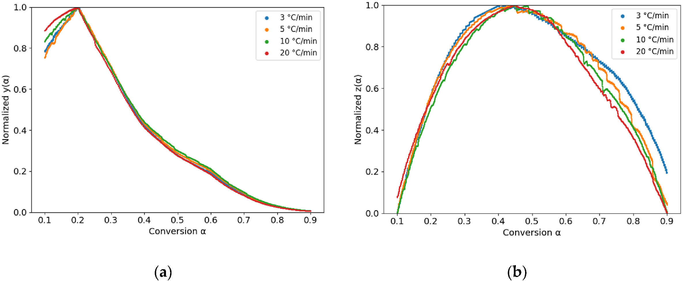
The maximum values of ,, and obtained respectively from the curing rate curve, y(α), and z(α) functions, are summarized in Table 3. According to [38], the autocatalytic model with two reacting factors m, n is applicable when < 0.632. To account for both autocatalytic and non-autocatalytic reaction pathways, the Kamal–Sourour (KS) kinetic model was employed [42]. The KS model can be expressed as follows:
where and represent the rate constants associated with the chemical-controlled and autocatalytic reactions, respectively; denotes the autocatalytic reaction order, and represents the overall reaction order with respect to the unreacted fraction.

Table 2.
Critical Curing Parameters of PU Determined from DSC at Heating Rates of 3, 5, 10, and 20 °C/min.
Table 2.
Critical Curing Parameters of PU Determined from DSC at Heating Rates of 3, 5, 10, and 20 °C/min.
| Heating rate | αp | αM | αp∞ |
|---|---|---|---|
| 3 °C/min | 0.325 | 0.201 | 0.421 |
| 5 °C/min | 0.381 | 0.200 | 0.448 |
| 10 °C/min | 0.407 | 0.200 | 0.450 |
| 20 °C/min | 0.389 | 0.198 | 0.450 |
Based on the global optimizer, the KS kinetic parameters were determined through robust nonlinear least-squares fitting using a soft L1 loss function [43]. This approach mitigates the impact of experimental noise in the DSC data, particularly at the extremities of the curves, resulting in stable and physically meaningful parameter estimates. Due to the rapid curing behavior of the PU system, the dataset collected at the highest heating rate was excluded from the fitting. To ensure computational stability and avoid negative values, the parameters were log-transformed. The robust loss optimization function was employed to minimize the residuals, with the objective function described using the soft L1 loss function, as defined below:
where denotes the residual of the -th data point, is the corresponding noise scale, and is a robust loss function introduced to reduce the influence of outliers.
The fitting curves are shown in Figure 5 and compared with the experimental data. The fitted DoC curves closely matched the experimental results, with values listed in Table 3, all exceeding 0.99. Overall, the values for the curing rate were consistently greater than 0.95, indicating high accuracy.
Table 3.
Correlation (R²) Between Degree of Cure and Curing Rate at Heating Rates of 3, 5, and 10 °C/min.
Table 3.
Correlation (R²) Between Degree of Cure and Curing Rate at Heating Rates of 3, 5, and 10 °C/min.
| Heating rate | R2 | |
| DOC | Curing rate | |
| 3 °C/min | 0.997 | 0.953 |
| 5 °C/min | 0.999 | 0.972 |
| 10 °C/min | 0.999 | 0.981 |
Based on the KS equation and fitted curves, the critical values of KS kinetics curing model are listed in Table 4.
3.2. Gelation
Time sweep oscillation tests were conducted at 50 °C with angular frequencies () of 1, 3, 10, 30, and 100 rad/s. Gel time can be estimated by measuring low-amplitude oscillatory shear and tracking changes in storage modulus (), loss modulus (), and complex viscosity (). To identify the gelation point for the PU system, three methods were considered: the crossover point between storage and loss modulus, the frequency-independent intersection of the dissipation factor , and the moment when viscosity becomes practically infinite [44]. For a typical thermoset, viscous behavior dominates in the early stages of curing ( > ). As the degree of crosslinking increases, there is often a rapid rise in elasticity, which begins to dominate the system ( > ). The intersection, = , is taken as the apparent gel point [45,46]. In some cases, no clear intersection point is observed within the measurement time window. This may be attributed to the characteristic timescale , which determines how long the material has to respond within each oscillation cycle (i.e. a shorter timescale means the material is “probed” more frequently). At low angular frequencies, the large timescale enables polymer chain relaxation, allowing the loss modulus to dominate longer into the cure. In such cases, gelation can be assessed using criteria based on the dissipation factor or complex viscosity. Of the five angular frequencies tested, crossover between the storage and loss modulus occurred only during the 100 rad/s trial, at approximately 200 s. This is not taken to be the gel point – rather, it is attributed to the very short deformation timescale (s) resulting in mildly elastic-dominant behavior as the polymer network rapidly began forming during the early stages of curing.
During the first 400-500 seconds of curing, the low magnitudes and close proximities of the storage and loss moduli in Figure 6 (a), coupled with experimental noise, led to significant instability in the dissipation factor for all trials. When computing for the curves in Figure 6 (b), and were first smoothed using a 3rd order Savitzky-Golay filter with a frame length of 21. Winter-Chambon theory states that, at the gel point, the storage and loss moduli grow proportionally as a function of frequency [47]. Therefore, the gel point can be identified by determining when the dissipation factor becomes independent of angular frequency. In Figure 6 (b), the most notable intersection occurs between 600-625 s, for which four of the five curves intersect. The 10 rad/s trial intersects most of the other curves slightly earlier, between 475-550 s. Thus, the crossover method indicates a gelation window of 475-625 s, during which the true gel point is likely to exist.
The final method is based on the premise that fully crosslinked networks exhibit a complex viscosity which diverges toward infinity. This method often relies on visual cues to identify the gel point, such as spikes or plateaus across various frequencies. No obvious features are present in Figure 6 (c) to indicate the gel point via this method – in linear or log scale. When mapping the selected points to the DoC curve under 50 °C in Figure 6 (d), the gelation point occurred around DoC = 0.53.
3.3. Glass Transition Temperatures
Three glass transition temperatures , , were measured for uncured resin, at gelation point, and cured resin, respectively. To determine as a function of conversion for a fast-curing PU system, an integrated approach was employed [10]. The procedure combines isothermal curing within a DSC, rapid quenching, and subsequent dynamic scanning. The conversion was calculated based on the residual enthalpy measured during the DSC analysis. All time references were synchronized to the DSC cell clock, effectively eliminating uncertainties related to sample preparation. The isothermal DSC test was conducted at 100 °C for 30 min, and the corresponding conversion curve is shown in Figure 7 (a). The PU system reached full cure at approximately 30 min under isothermal conditions. The time–temperature–transformation (TTT) diagram was constructed based on the Di Benedetto equation. The fitted glass transition temperature as a function of time is shown in Figure 7 (b), with the fitted constant of approximately 0.31. Similar calorimetry-based characterization and construction of TTT-type processing diagrams have been reported for fast-curing polyurethane adhesives to support model calibration and process-window definition [14].
3.4. Molecular Dynamic Simulation capturing Tg
To compare the MD model with experiment, the unreactive PU system was heated to 100 °C as previously described. The DoC vs step time curve is plotted by Figure 8 (a). Crosslinking was rapid in the beginning, followed by a gradual slowing until it reached 0 due to the limit of the reactive functional groups. The curing rate from MD simulation was normalized and compared to the curing rate with the experimental curve, which is shown in Figure 8 (b). The curing rates were mapped to each DoC point, the experimental curve shows a higher reaction rate happened in the beginning of the reaction compared to the MD curve, which shows the isocyanate–hydroxyl reaction is highly reactive, with reaction sites achieving instantaneous and complete contact [48,49]. By comparing the curing-rate trends of the two groups, it was observed that chemical reactions dominate the cross-linking process during curing. To evaluate the of the MD model, 10 DoC points were selected: 0.2, 0.3, 0.4, 0.65, 0.7, 0.75, 0.8, 0.85, 0.95 and 0.97. was determined from the heating-induced specific volume temperature curves by identifying the intersection of the linear fits to the glassy and rubbery regimes and 5 curves of different DoC models are presented by Figure 8 (c). As the degree of cure increases, the specific volume of the polymer systematically decreases, reflecting the progressive formation of a denser crosslinked network and the reduction of free volume.
The resulting – relationship is shown in Figure 8 (d). The extracted data were fitted using the DiBenedetto equation, with the initial and fully cured values fixed. The fitted curve shows excellent agreement with the MD data, yielding a high coefficient of determination (), indicating that the DiBenedetto model effectively captures the evolution of with DoC.
A GPR-based predictive framework was implemented to robustly model the DiBenedetto relationship, while explicitly accounting for experimental and MD noise through additive noise terms.
3.5. Gaussian Process Regression Prediction
To fit the predictive model, in total 16 data points were combined from experimental and MD data, a cross validation was performed by k-fold cross validation method (k = 5), and the fitted curve is plotted as the blue dash line in Figure 9. The noise-based weighting controls both the data influence on the mean prediction and the width of the confidence interval. The best global fitted λ = 0.275 was selected by cross validation with the lowest RMSE in the defined region. This model captures the globally monotonic increasing behavior of Tg with DoC and strictly satisfies the predefined physical endpoints at DoC = 0 and 1.
By superimposing GP residuals onto the DiBenedetto baseline, the proposed model (solid orange curve) effectively corrects these local deviations (systematic and random noises) while preserving the physically meaningful trends imposed by the baseline and hard boundary constraints. The GPR correction primarily acted on regions where experimental and MD data persistently deviate from the baseline between 0.3 and 0.6, thereby enhancing data consistency across the entire DoC range without introducing non-physical oscillations. Notably, the model avoids overfitting sparse regions of the dataset, as evidenced by the final curve's smoothness and the absence of abnormal curvature near the endpoints. The wider 95 % confidence interval bands observed at low and intermediate degrees of cure arise from sparse experimental measurements and the relatively higher noise assigned to the MD data, where the automatically selected noise levels were 0.4 for MD and 0.4 for experiments. The predicted curve captures the theory-guided DiBenedetto trend well, and the model incorporates a reliable treatment of measurement and simulation noise.
4. Conclusions
In this study, the curing behavior of the PU system was characterized using thermal and rheological measurements conducted by DSC and a rheometer. The apparent Ea determined using the isoconversional method was 46.12 kJ/mol. A KS curing kinetics model was established to describe the curing evolution. In addition, the gelation point was identified based on combined DSC and rheological measurements, corresponding to a DoC of approximately 0.53.
Due to the rapid curing behavior of the PU system, the Tg was determined using a combination of experimental measurements and MD simulations. At the molecular scale, MD simulations were performed using LAMMPS, from which the corresponding Tg values were extracted at different DoC. GPR was employed as a bridging framework to integrate experimental DSC data and MD results, with crossvalidation used to ensure predictive robustness. A topological crosslinking approach was implemented in LAMMPS under different temperature conditions, from which a global DiBenedetto parameter of λ = 0.28 was determined. GPR enabled reliable forecasting the trend of Tg – α combined MD and experimental results with CI regions indicate DoC ranges dominated by MD data and limited experimental constraints. Furthermore, GP residuals effectively capture systematic, physics-driven biases in the Tg relationship, biases that cannot be fully described by the DiBenedetto model alone. In the Tg – α relationship, systematic, physics-driven biases exist that cannot be fully described by the DiBenedetto model alone.
Author Contributions
Conceptualization, L.W., M.B. and J.H.; methodology, L.W., J.H. and S.M.; software, L.W.; formal analysis, L.W.; investigation, L.W., J.H., and M.B.; data curation, L.W. and S.M.; writing—original draft preparation, L.W., J.H., S.G., S.M., M.B.; writing—review and editing, L.W., J.H., S.G., S.M., M.B., A.T. and A.Z.; visualization, L.W., J.H, and S.G.; supervision, M.B., A.Z. and A.T.; project administration, M.B, A.T., A.Z.; funding acquisition, M.B. and A.T. All authors have read and agreed to the published version of the manuscript.
Funding
The research is funded within the Department of Energy DE-EE0011184 Project entitled “Pultrusion of structural components made of lignin-based carbon fiber”.
Institutional Review Board Statement
Not applicable
Data Availability Statement
Data are contained within the article
Conflicts of Interest
The authors declare no conflict of interest.
Abbreviations
The following abbreviations are used in this manuscript:
| PU | Polyurethane |
| Tg | Glass transition temperature |
| DSC | Differential scanning calorimetry |
| TMA | Thermomechanical analysis |
| DoC | Degree of cure |
| MD | Molecular dynamics |
| EMC | Enhanced Monte Carlo |
| ML | Machine learning |
| GPR | Gaussian Process Regression |
| CTE | Coefficient of thermal expansion |
| OPLS-AA | Optimized potentials for liquid simulation all atom |
| COMPASS | Condensed-phase Optimized Molecular Potential for Atomistic Simulation Studies |
| PCFF | Polymer consistent force field |
| NPT | Constant Number of particles, Pressure, and Temperature |
| RMSE | Root mean square error |
| KS | Kamal–Sourour |
| TTT | Time–temperature–transformation |
References
- De Souza, Felipe M; Kahol, Pawan K; Gupta, Ram K. Introduction to polyurethane chemistry. In Polyurethane chemistry: Renewable polyols and isocyanates; ACS Publications, 2021; pp. pages 1–24. [Google Scholar]
- Heath, Daniel E.; Cooper, Stuart L. A - polyurethanes. In Biomaterials Science (Third Edition), third edition edition; Ratner, Buddy D., Hoffman, Allan S., Schoen, Frederick J., Lemons, Jack E., Eds.; Academic Press, 2013; pp. pages 79–82. [Google Scholar]
- Wienen, David; Gries, Thomas; Cooper, Stuart L; Heath, Daniel E. An overview of polyurethane biomaterials and their use in drug delivery. Journal of Controlled Release 2023, 363, 376–388. [Google Scholar] [CrossRef]
- Das, Abhijit; Mahanwar, Prakash. A brief discussion on advances in polyurethane applications. Advanced Industrial and Engineering Polymer Research 2020, 3(3), 93–101. [Google Scholar] [CrossRef]
- Mukherji, Arindam; Njuguna, James. An assessment on effect of process parameters on pull force during pultrusion. The International Journal of Advanced Manufacturing Technology 2022, 121(5), 3419–3438. [Google Scholar] [CrossRef]
- Irfan, Muhammad S; Shotton-Gale, Nicholas; Paget, Mark A; Machavaram, Venkata R; Leek, Colin; Wootton, Shane; Hudson, Mark; Helsmans, Stefan; Bogonez, Francisco N; Pandita, Surya D; et al. A modified pultrusion process. Journal of Composite Materials 2017, 51(13), 1925–1941. [Google Scholar] [CrossRef]
- Baran, Ismet; Tutum, Cem C; Nielsen, Michael W; Hattel, Jesper H. Process induced residual stresses and distortions in pultrusion. Composites Part B: Engineering 2013, 51, 148–161. [Google Scholar] [CrossRef]
- Venditti, RA; Gillham, JK. A relationship between the glass transition temperature (tg) and fractional conversion for thermosetting systems. Journal of Applied Polymer Science 1997, 64(1), 3–14. [Google Scholar] [CrossRef]
- Ramis, X; Cadenato, A; Morancho, JM; Salla, JM. Curing of a thermosetting powder coating by means of dmta, tma and dsc. Polymer 2003, 44(7), 2067–2079. [Google Scholar] [CrossRef]
- Teil, H; Page, SA; Michaud, V; Månson, J-AE. Ttt-cure diagram of an anhydridecured epoxy system including gelation, vitrification, curing kinetics model, and monitoring of the glass transition temperature. Journal of Applied Polymer Science 2004, 93(4), 1774–1787. [Google Scholar] [CrossRef]
- Gu, Yuwei; Zhao, Julia; Johnson, Jeremiah A. Polymer networks: from plastics and gels to porous frameworks. Angewandte Chemie International Edition 2020, 59(13), 5022–5049. [Google Scholar] [CrossRef] [PubMed]
- Imrie, Patrick; Jin, Jianyong. Gelation of raft polymer networks analyzed by rheology. Polymer 2025, 317, 127956. [Google Scholar] [CrossRef]
- Karim Boulkadid, Moulai; Touidjine, Sabri; Tra che, Djalal; Belkhiri, Samir. Analytical methods for the assessment of curing kinetics of polyurethane binders for high-energy composites. Critical Reviews in Analytical Chemistry 2022, 52(5), 1112–1121. [Google Scholar] [CrossRef]
- Jennrich, Rebecca; Lion, Alexander; Johlitz, Michael; Ernst, Sarah; Dilger, Klaus; Stammen, Elisabeth. Thermomechanical characterization and modeling of fast-curing polyurethane adhesives. Continuum Mechanics and Thermodynamics 2020, 32(2), 421–432. [Google Scholar] [CrossRef]
- Han, Jie; Gee, Richard H; Boyd, Richard H. Glass transition temperatures of polymers from molecular dynamics simulations. Macromolecules 1994, 27(26), 7781–7784. [Google Scholar] [CrossRef]
- in’t Veld, Pieter J; Rutledge, Gregory C. Temperature-dependent elasticity of a semicrystalline interphase composed of freely rotating chains. Macromolecules 2003, 36(19), 7358–7365. [Google Scholar] [CrossRef]
- Seeger, Matthias. Gaussian processes for machine learning. International journal of neural systems 2004, 14(02), 69–106. [Google Scholar] [CrossRef]
- Wang, Jie. An intuitive tutorial to gaussian process regression. Computing in Science & Engineering 2023, 25(4), 4–11. [Google Scholar] [CrossRef]
- Flory, Paul J. Molecular size distribution in three dimensional polymers. v. postgelation relationships. Journal of the American Chemical Society 1947, 69(1), 30–35. [Google Scholar] [CrossRef]
- Lang, Michael; Muller, T. Analysis of the gel point of polymer model networks by computer simulations. Macromolecules 2020, 53(2), 498–512. [Google Scholar] [CrossRef]
- Li, X; Nakagawa, S; Tsuji, Y; Watanabe, N; Shibayama, M. Polymer gel with a flexible and highly ordered three-dimensional network synthesized via bond percolation. Science advances 2019, 5(12), eaax8647. [Google Scholar] [CrossRef]
- Zhang, Chao; Li, Yi; Wu, Yongshen; Wang, Cuixia; Liang, Jian; Xu, Zihan; Zhao, Peng; Wang, Jing. Key role of cross-linking homogeneity in polyurethane mechanical properties: Insights from molecular dynamics. The Journal of Physical Chemistry B 2024, 128(50), 12612–12627. [Google Scholar] [CrossRef]
- Hadipeykani, Majid; Aghadavoudi, Farshid; Toghraie, Davood. A molecular dynamics simulation of the glass transition temperature and volumetric thermal expansion coefficient of thermoset polymer based epoxy nanocomposite reinforced by cnt: a statistical study. Physica A: Statistical Mechanics and its Applications 2020, 546, 123995. [Google Scholar] [CrossRef]
- Zheng, Tianze; Li, Ting; Shi, Jiaxin; Wu, Tianyu; Zhuang, Zhuo; Xu, Jun; Guo, Baohua. Molecular insight into the toughness of polyureas: A hybrid all atom/coarse-grained molecular dynamics study. Macromolecules 2022, 55(8), 3020–3029. [Google Scholar] [CrossRef]
- Olejnik, Adrian; Gosz, Kamila; Piszczyk, Łukasz. Kinetics of cross-linking processes of fast-curing polyurethane system. Thermochimica Acta 2020, 683, 178435. [Google Scholar] [CrossRef]
- Molecular Massively Parallel Simulator. Lammps. 2013. Available online: http://lammps.sandia.gov.
- Fried, J.R.; Li, B. Atomistic simulation of the glass transition of di-substituted polysilanes. Computational and Theoretical Polymer Science 2001, 11(4), 273–281. [Google Scholar] [CrossRef]
- Sun, H.; Ren, P.; Fried, J.R. The com-pass force field: parameterization and validation for phosphazenes. Computational and Theoretical Polymer Science 1998, 8(1), 229–246. [Google Scholar] [CrossRef]
- DiBenedetto, AT. Prediction of the glass transition temperature of polymers: a model based on the principle of corresponding states. Journal of Polymer Science Part B: Polymer Physics 1987, 25(9), 1949–1969. [Google Scholar] [CrossRef]
- Duvenaud, David. The kernel cookbook: Advice on covariance functions. 2014. Available online: https://www.
- Ameli, Siavash; Shadden, Shawn C. Noise estimation in gaussian process regression. arXiv 2022, arXiv:2206.09976. [Google Scholar] [CrossRef]
- Anguita, Davide; Ghelardoni, Luca; Ghio, Alessandro; Oneto, Luca; Ridella, Sandro; et al. The’k’in k-fold cross validation. Esann 2012, volume 102, 441–446. [Google Scholar]
- Qiu, Chunfu. Nonparametric regression and generalized linear models: a roughness, penalty approach; 1995. [Google Scholar]
- Bishop, Christopher M; Nasrabadi, Nasser M. Pattern recognition and machine learning; Springer, 2006; volume 4. [Google Scholar]
- Navarro-García, Manuel; Guerrero, Vanesa; Durban, María. On constrained smoothing and out-of-range prediction using p-splines: A conic optimization approach. Applied Mathematics and Computation 2023, 441, 127679. [Google Scholar] [CrossRef]
- Yousefi, A; Lafleur, Pierre G; Gauvin, Raymond. Kinetic studies of thermoset cure reactions: a review. Polymer Composites 1997, 18(2), 157–168. [Google Scholar] [CrossRef]
- D Ro¸su, CN Ca¸scaval; Mustatˇa, F.; Ciobanu, C. Cure kinetics of epoxy resins studied by non-isothermal dsc data. Thermochimica Acta 2002, 383(1-2), 119–127. [Google Scholar] [CrossRef]
- Málek, Jiří. Kinetic analysis of non-isothermal calorimetric data; 1996. [Google Scholar]
- Málek, Jiří. Kinetic analysis of crystallization processes in amorphous materials. Thermochimica Acta 2000, 355(1-2), 239–253. [Google Scholar] [CrossRef]
- Senum, GI; Yang, RT. Rational approximations of the integral of the arrhenius function. Journal of thermal analysis 1977, 11(3), 445–447. [Google Scholar] [CrossRef]
- Vyazovkin, Sergey. Isoconversional kinetics of thermally stimulated processes; Springer, 2015. [Google Scholar]
- Kamal, MR; Sourour, S. Kinetics and thermal characterization of thermoset cure. Polymer Engineering & Science 1973, 13(1), 59–64. [Google Scholar] [CrossRef]
- Dennis, John E, Jr.; Welsch, Roy E. Techniques for nonlinear least squares and robust regression. Communications in Statistics-simulation and Computation 1978, 7(4), 345–359. [Google Scholar] [CrossRef]
- Gazo Hanna, Eddie; Younes, Khaled; Amine, Semaan; Roufayel, Rabih. Exploring gel-point identification in epoxy resin using rheology and unsupervised learning. Gels 2023, 9(10), 828. [Google Scholar] [CrossRef] [PubMed]
- Lange, J; Altmann, N; Kelly, CT; Halley, PJ. Understanding vitrification during cure of epoxy resins using dynamic scanning calorimetry and rheological techniques. Polymer 2000, 41(15), 5949–5955. [Google Scholar] [CrossRef]
- Cai, Jianfen J; Salovey, Ronald. Chemorheology of model filled rubber compounds during curing. Polymer Engineering & Science 2001, 41(11), 1853–1858. [Google Scholar] [CrossRef]
- Winter, H Henning; Chambon, Francois. Analysis of linear viscoelasticity of a crosslinking polymer at the gel point. Journal of rheology 1986, 30(2), 367–382. [Google Scholar] [CrossRef]
- Ionescu, Mihail. Chemistry and technology of polyols for polyurethanes; iSmithers Rapra Publishing, 2005. [Google Scholar]
- Gertig, Christoph; Erdkamp, Eric; Ernst, Andreas; Hemprich, Carl; Kr¨oger, Leif C; Langanke, Jens; Bardow, Andr´e; Leonhard, Kai. Reaction mechanisms and rate constants of auto-catalytic urethane formation and cleavage reactions. ChemistryOpen 2021, 10(5), 534–544. [Google Scholar] [CrossRef] [PubMed]
Figure 1.
MD simulation schematic of PU network formation and Tg characterization.
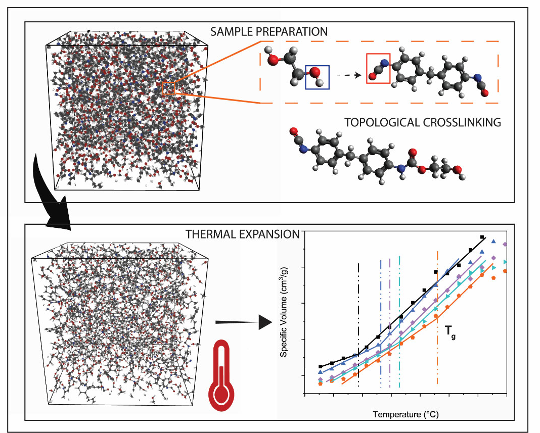
Figure 2.
Dynamic heat flow results of PU within (a) time; (b) temperature under 3, 5, 10, and 20 C/min heating rates.
Figure 2.
Dynamic heat flow results of PU within (a) time; (b) temperature under 3, 5, 10, and 20 C/min heating rates.
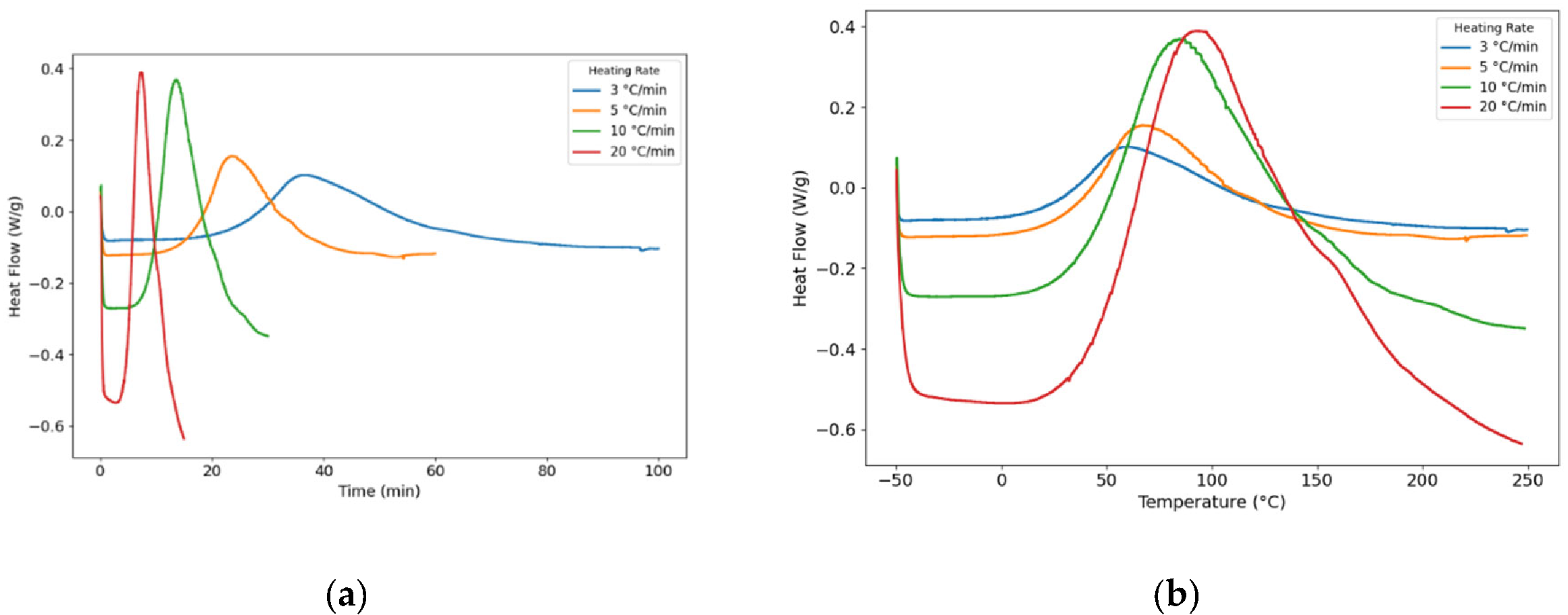
Figure 3.
(a) Experimentally Determined Degree of Cure of PU; (b) Curing rate curves for PU under 5, 10, and 20 °C/min heating rates.
Figure 3.
(a) Experimentally Determined Degree of Cure of PU; (b) Curing rate curves for PU under 5, 10, and 20 °C/min heating rates.
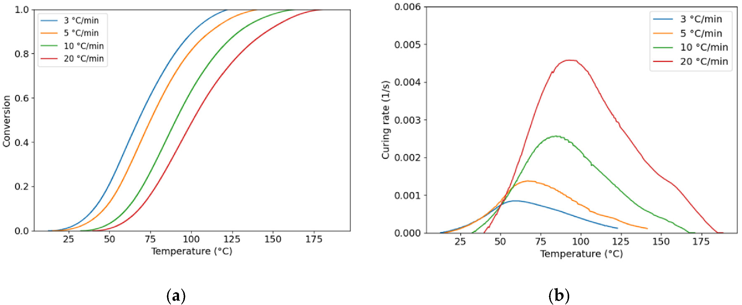
Figure 5.
Fitted curves of (a) degree of cure and (b) curing rate for the PU system.
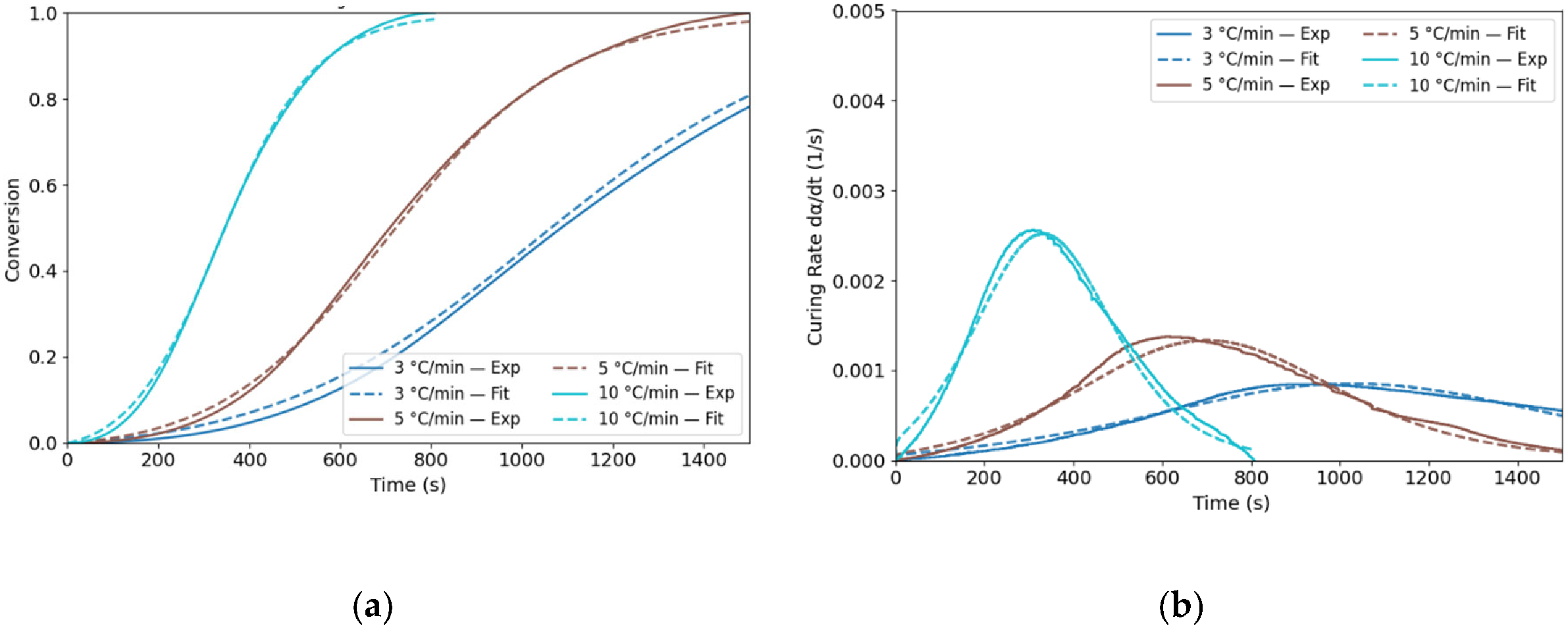
Figure 6.
(a) Storage and loss modulus, (b) dissipation factor, and (c) complex viscosity versus time at angular frequencies of 1, 3, 10, 30, and 100 rad/s and a temperature of 50 °C; (d) DoC versus time at 50 °C isothermally from DSC.
Figure 6.
(a) Storage and loss modulus, (b) dissipation factor, and (c) complex viscosity versus time at angular frequencies of 1, 3, 10, 30, and 100 rad/s and a temperature of 50 °C; (d) DoC versus time at 50 °C isothermally from DSC.
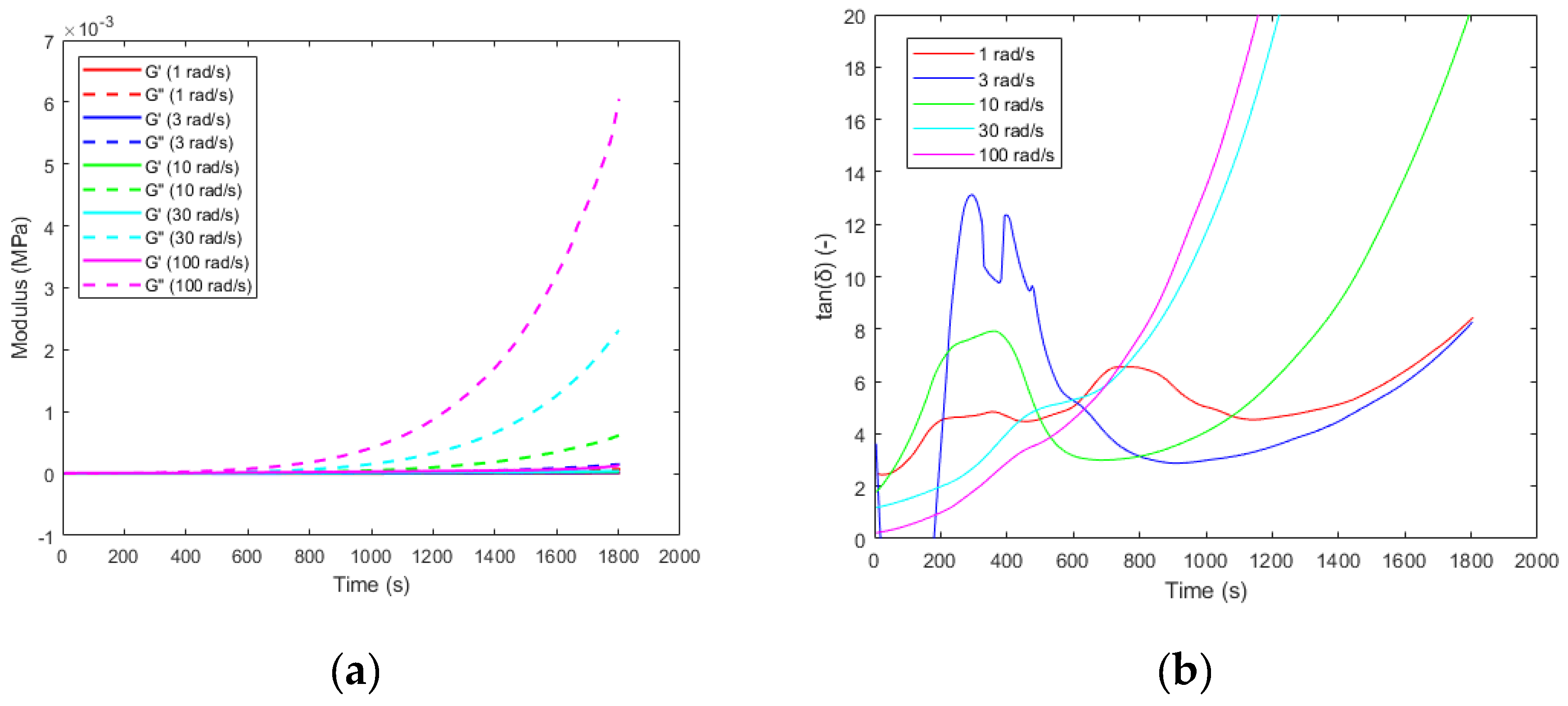
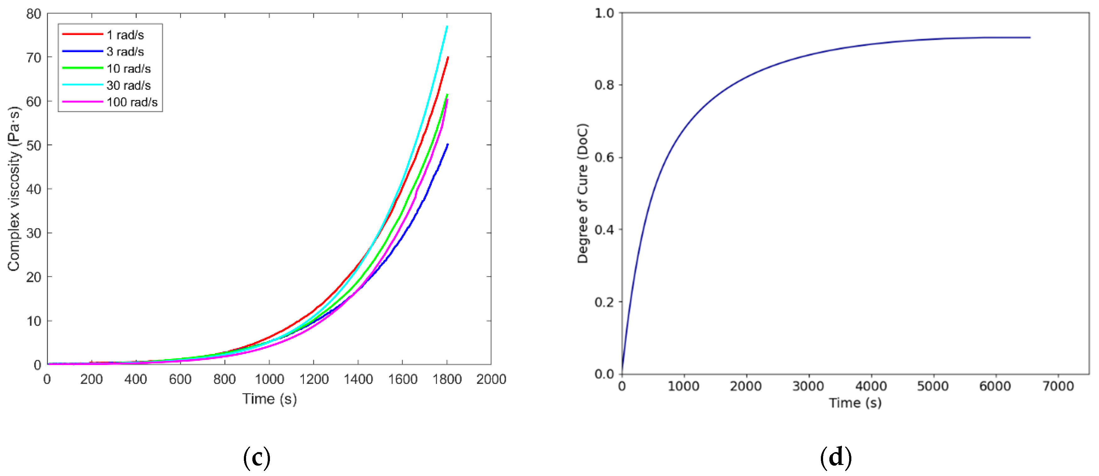
Figure 7.
(a) Conversion Curve; (b) Tg fitting curve of PU under Isothermal Conditions at 100 °C
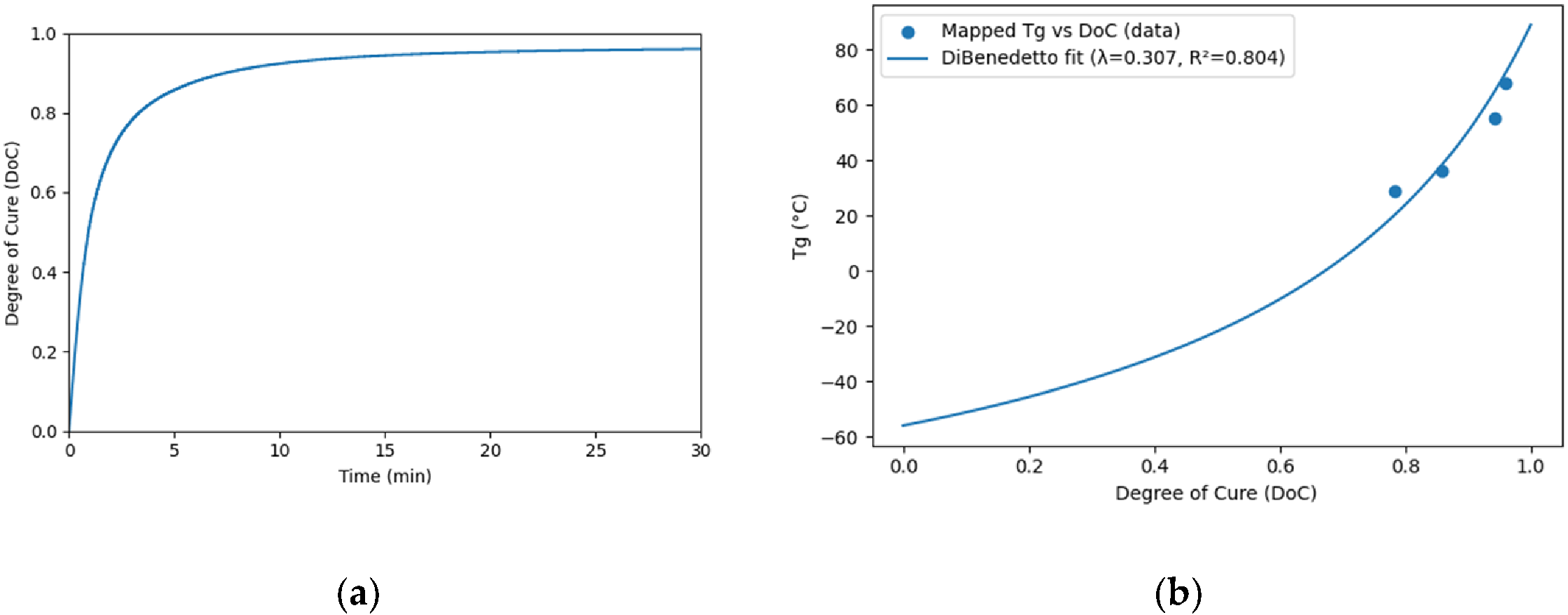
Figure 8.
(a) Conversion Curve from MD simulation; (b) Comparison of curing rates between experimental measurements and MD simulations; (c) Thermal expansion measurement with different DoC models; (d) Fitted DiBenedetto curve from MD simulations.
Figure 8.
(a) Conversion Curve from MD simulation; (b) Comparison of curing rates between experimental measurements and MD simulations; (c) Thermal expansion measurement with different DoC models; (d) Fitted DiBenedetto curve from MD simulations.
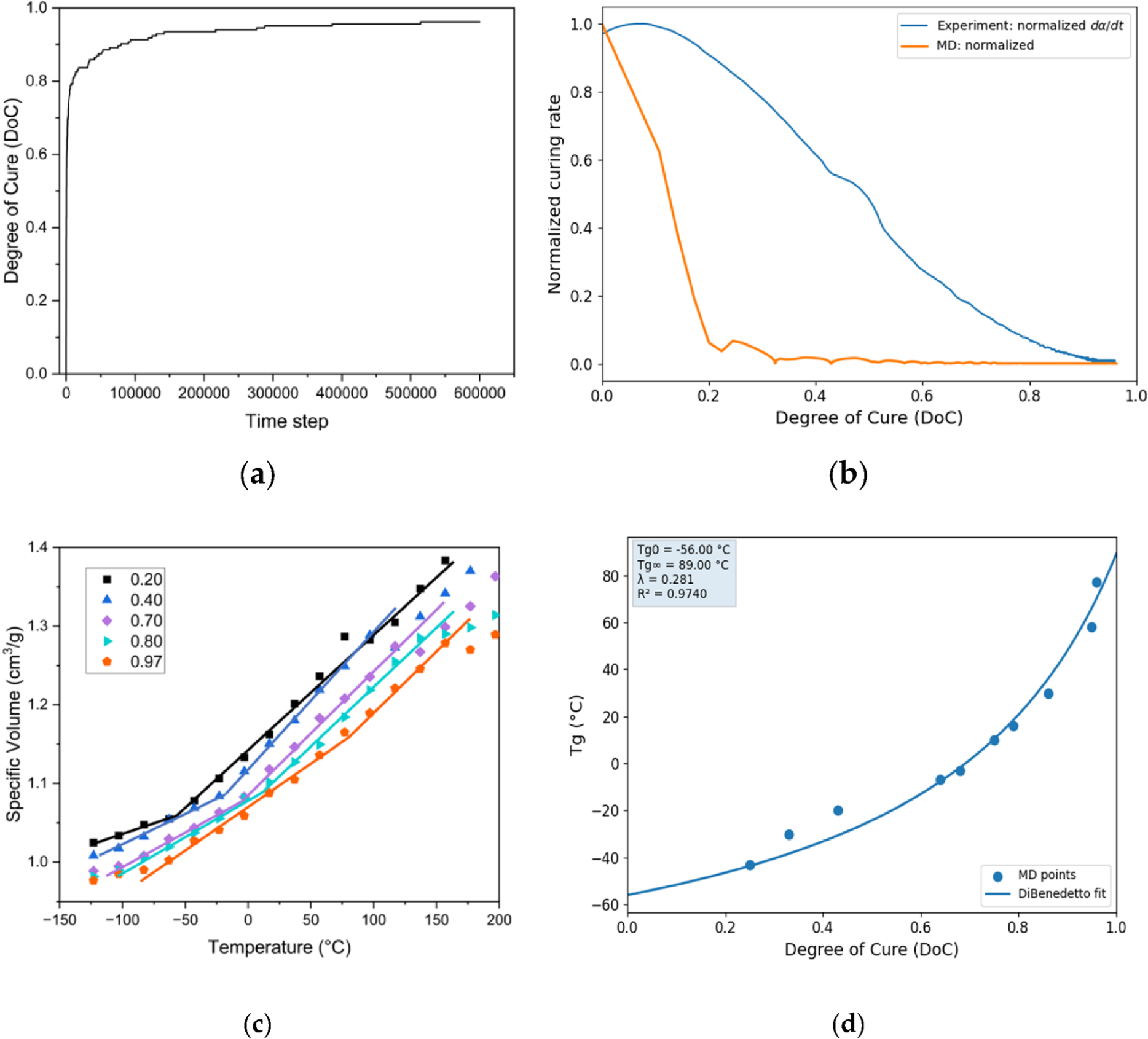
Figure 9.
Predictions from the DiBenedetto model for PU augmented with GPR.
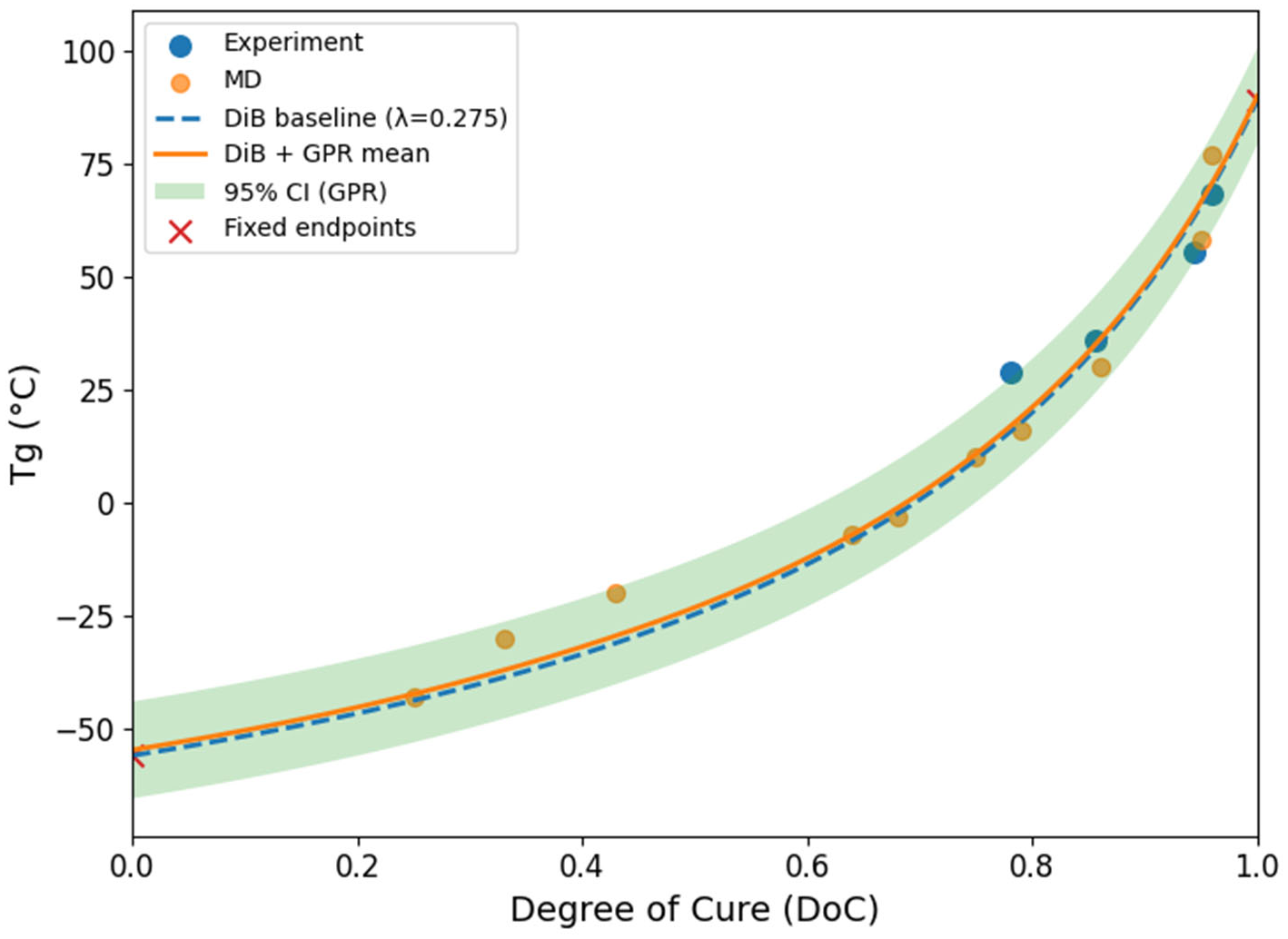
Table 1.
Curing Kinetics of PU Derived from DSC Measurements Conducted at 3, 5, 10, and 20 °C/min.
| Tonset (°C) | Tp (°C) | Tendset (°C) | Curing duration (min) | ∆H (J/g) | |
|---|---|---|---|---|---|
| 3 °C/min | 12.70 | 59.12 | 122.81 | 35.12 | 108.34 |
| 5 °C/min | 20.39 | 67.50 | 183.53 | 25.17 | 112.28 |
| 10 °C/min | 40.74 | 84.60 | 169.89 | 13.81 | 149.64 |
| 20 °C/min | 37.37 | 93.80 | 142.42 | 7.40 | 119.63 |
Table 4.
Critical values of PU evaluated from DSC recorded at 3, 5, and 10 °C/min heating rates.
| Resin | A1 | A2 | m | n | Ea (kJ/mol) | R2 |
| PU | 1.002e-2 | 3.516e4 | 0.110 | 1.6384 | 46.12 | 0.97 |
Disclaimer/Publisher’s Note: The statements, opinions and data contained in all publications are solely those of the individual author(s) and contributor(s) and not of MDPI and/or the editor(s). MDPI and/or the editor(s) disclaim responsibility for any injury to people or property resulting from any ideas, methods, instructions or products referred to in the content. |
© 2026 by the authors. Licensee MDPI, Basel, Switzerland. This article is an open access article distributed under the terms and conditions of the Creative Commons Attribution (CC BY) license (http://creativecommons.org/licenses/by/4.0/).
Copyright: This open access article is published under a Creative Commons CC BY 4.0 license, which permit the free download, distribution, and reuse, provided that the author and preprint are cited in any reuse.


