Submitted:
30 January 2026
Posted:
03 February 2026
You are already at the latest version
Abstract
The Novais climate classification is a system that employs reanalysis climate data and integrates both analytical and dynamic approaches to define homogeneous climate units according to the adopted hierarchical scale. This study applies the Novais classification globally, contributing to traditional, exclusively empirical climate classification systems widely used in the globe. Its methodology relies on cartographic products that were generated on the free software Dinamica EGO, associating spatial and non-spatial data through conditional equations. The Novais climate classification system contains hierarchies ranging from the zonal to the local scale, encompassing the regional level for the study area that comprises units divided into climatic zone, zonal climate, climatic domain, climatic subdomain, and climatic region. This study found 11 climatic domains, characterized by the average temperature of the coldest month: equatorial, mild equatorial, tropical, mild tropical, subtropical, temperate, cold temperate, subglacial, glacial, semiarid, and arid. These domains are subdivided into climatic subdomains according to the number of dry months (which can be humid, semihumid, semidry, and dry). Finally, the arrangement of domains and subdomains defines climatic regions by considering variations in relief and the biogeographic regions of each continent. Research at this scale can enhance the understanding of global climates, providing a relevant analytical and dynamic diagnosis that can synthesize the diversity and complexity of the climate across all continents.
Keywords:
Novais climate classification system
; climate characterization
; cartographic modeling
1. Introduction
Earth receives intense solar radiation due to its position within the solar system. This factor, combined with the presence of liquid water, favors the emergence and maintenance of life. Climatic elements, such as temperature, precipitation, and atmospheric pressure, exhibit spatial variability influenced by latitude, altitude, topography, proximity to oceans, vegetation cover, and anthropogenic activities. These climatic factors actively shape terrestrial landscapes through diverse weathering processes. According to the World Meteorological Organization (WMO), climate normals are calculated based on 30-year averages of atmospheric conditions, reflecting their critical role in maintaining ecological balance and supporting societal planning.
Climate classifications are essential for addressing climatic diversity and are generally divided into two main categories: analytical, which focus on climatic elements and their effects on the biosphere, and dynamic, which emphasize variability in air masses. While several classification models have emerged from these approaches, historical limitations in data quality have affected their accuracy.
Novais (2019) has proposed a hybrid climate classification system that integrates analytical and dynamic methods using climate reanalysis data, multivariate statistics, and cartographic modeling. Initially developed for the Cerrado biome, this system has been expanded to assess climates across Brazil, South America, Europe, and, more recently, the entire globe, thereby enhancing multi-scale analyses and improving environmental management. This methodology is distinguished by its incorporation of recent technological and methodological advancements. In this paper, the classification method is detailed, followed by the presentation of Novais’s Global Climate Map.
2. Methods
The hybrid Novais system employs a hierarchical structure that classifies climates from the most comprehensive to the most specific levels. Understanding the interaction between different scales and hierarchical levels is essential to comprehending climate impacts on a given area. The order of magnitude of climate scales, as defined by Ribeiro (1993), Galvani (2020), and Fialho et al. (2023), is summarized in Table 1.
The first levels of Novais’s hierarchy are found at the zonal climate scale, represented by climate zones and zonal climates, which span continents. These classes are primarily organized by latitude, atmospheric circulation centers, and regional geographic factors. The tilt of the Earth’s axis relative to its orbit causes seasonal variations in the angle of solar incidence, most notably during the solstices (Novais, 2019). Based on this phenomenon, Novais’ climate classification establishes climatic zones, the first hierarchy, according to the angle of solar incidence on the Earth.
As shown in Figure 1, the solar “illumination cone” on the intertropical region has a range of 46°54’ during equinoxes, shifting to the hemispheres at solstices, indicating the zones of maximum solar incidence in the summer. To improve the delimitation of these zones, Novais (2023) proposed four new imaginary lines in addition to the traditional ones.
Subequatorial lines, situated at 11°43’30” latitude in both hemispheres, represent an intermediate position between the equator and the tropics. The subtropic lines, at 46°54’ latitude, indicate the greatest solar insolation during the solstices, in which the Sun reaches a zenith angle of 23°27’ (solar noon) over the tropics. These new references enrich the analysis of solar energy distribution and the definition of climatic zones.
The five climatic zones delimited by these imaginary lines, according to Novais (2023a), are shown in Table 2.
Zonal climates, defined in the second hierarchy of Novais’ classification system, differ from climatic zones in that they are based on mean temperature of the coldest month (MTCM), a parameter closely related to solar radiation (Novais 2023a). The isotherms delimiting them were proposed by Novais (2017) — some of which were based on Köppen (1948) — considering factors such as population thermal sensitivity, tropical diseases, frost formation, and snow (Novais and Machado 2023a):
- Very hot (torrid) - MTCM above 22.5 °C, equatorial populations’ sensitivity to cold;
- Hot - MTCM from 15.1 to 22.5 °C, with Frost occurrence possible at the transition to the moderate zonal climate;
- Moderate - MTCM from 0.1 to 15 °C, with sporadic frosts and low presence of diseases transmitted by tropical vectors;
- Cold - MTCM from -14.9 to 0 °C; possibility of snow cover;
- Polar - MTCM ≤ −15 °C and soil freezing.
In addition to zonal climates, the second hierarchy includes azonal climates, which are common in mountainous areas between the subtropics and associated with the adiabatic effect. Novais and Machado (2023) define a climate as azonal when its MTCM corresponds to that of two zonal climates colder than the climatic zone in which it is located.
The regional climate scale has the greatest degree of hierarchical variation, as it connects the upper and lower levels. It includes three climate hierarchies: climatic domain, subdomain, and region. These hierarchies are defined by secondary circulation and regional geographic characteristics, considering criteria such the mean temperature of the coldest month (MTCM), precipitation, the number of dry months (precipitation below potential evapotranspiration), and continental location, particularly terrain features.
Climatic domains (Table 3) subdivide zonal climates based on the MTCM intervals, while also incorporating the influence of regional atmospheric systems, such as the Intertropical Convergence Zone (ITCZ). Thus, even with identical MTCMs, domains such as equatorial and tropical are distinguished by their seasonal moisture regimes (Novais 2023a). Moreover, semiarid and arid domains are defined by 12 dry months per year and average annual precipitations above or below 500 mm (Novais and Machado 2023b).
The fourth hierarchy, climatic subdomains, is based on the number of dry months per year, with the climatological water balance and ETp calculated by Penman-Monteith method (1964), which is more comprehensive than that of Thornthwaite and Mather (1955). A month is classified as dry when precipitation (P) is lower than ETp, producing a soil water deficit, reducing surface runoff, and constraining plant growth.
According to Novais and Galvani (2022), ETp is related to atmospheric attributes, whereas real evapotranspiration depends on soil moisture. Water surplus indicates the volume of water available during the period, while P–ETp represents the potential water balance. Based on these criteria (Table 4), the subdomains are classified according to the number of dry months as humid, semihumid, semidry, and dry (Novais and Machado 2023).
Average temperature, precipitation, and ETp data from 1981 to 2010, obtained from CHELSA (Climatologies at high resolution for the earth’s land surface areas) version 2.1 (Karger et al. 2018), were used to define climatic domains and subdomains. CHELSA offers high-resolution global data (one km²), integrating ERA-Interim climate reanalyses with information from more than 26,000 meteorological stations and measurements from ships, aircraft, probes, and satellites. Although broadly comprehensive, CHELSA does not provide ETp or mean temperature data for Antarctica. To fill this gap, we used version 1.2 data for average temperature (1979–2013) and version 2.1 data for precipitation to delineate the Antarctic climatic subdomains (www.chelsa-climate.org).
Novais’ (2019) methodology was implemented through an automated model developed in Dinamica EGO software, which enabled rapid processing of climate data (Figure 2). Climatic domains were delimited based on the MTCM values, which obtained by finding the coldest pixel in the monthly rasters and generating a combined raster. These values are reclassified according to Chart 3 and cross-referenced with ITCZ activity, the number of dry months, and average annual precipitation. ITCZ is essential to distinguish the equatorial and tropical domains that share the same MTCM band.
ITCZ stands on the ascending branch of the Hadley Cell, varying seasonally from 8 to 1°N (Hastenrath and Heller, 1977, Citeau et al. 1988). More recent studies indicate that it can extend beyond 5°S, forming a double band with maximum precipitation in April in South America (Teodoro et al. 2019, Cavalcanti et al. 2009). In this study, its delimitation considers three main criteria: (1) limits in Brazil according to Novais and Machado (2023); (2) humid tropical forests between the subequators according to Olson et al. (2001); and (3) precipitation above 150 mm in April in the southern hemisphere and in October in the northern hemisphere as these months represent tropical seasonal transitions.
The climatic subdomains were delineated using a condicioning logic model wich aggregates the total number of dry months in a year and reclassified the resultant raster according to the criteria in Table 4. Finally, the domain and subdomain raster maps were converted into shapefiles using ArcGIS 10.8 software and overlaid into a single file with the climate attributes. Visualization was standardized by a symbology defined by colors and tones.
Climatic regions, defined as the fifth level of the classification hierarchy, integrate domains and subdomains within continents by accounting for topography, bioclimatic zones, and distance from the ocean, alongside meteorological factors such as frost frequency, imparting them a hybrid character. This delineation resolves the occurrence of the same climate type across different parts of the globe.
The lower level of the climate scale holds a more direct influence on surface and is divided into subregional and local scales. The subregional scale encompasses the climatic subregion and the mesoclimate -the sixth and seventh hierarchies in Novais’s system- with spatial extents ranging from tens to thousands of square kilometers. The primary criteria rely on instrumental measurements. Key organizing factors at this scale include geoecological integration, human activity, and urban planning, while delimitation is typically based on geomorphological units. The eighth hierarchy is occupied by topoclimates/local climates, with restricted occurrence in the relief, such as on slopes exposed to insolation, local wind circulation, and orographic precipitation, as well as urban local climates influenced by different land uses
Only the upper level of Novais’s classification system was applied at the global scale in this paper. This level includes the hierarchies of climatic zones, zonal climates, climatic domains and subdomains.
To facilitate the interpretation of the climatic classes, a coding scheme was developed to represent each unit in a concise and systematic manner. Figure 3 illustrates this structure according to the example of the Semi-dry Tropical of Southern Central Brazil. In this scheme, the climatic domain is denoted by two uppercase letters (e.g., Tr for tropical), while the subdomain is indicated by specific symbols - (“) for humid, (‘) for semihumid, (*) for semidry, and (**) for dry - reflecting the number of dry months. The climatic region is expressed by three lowercase letters (e.g., scb, referring to southern central Brazil), which identify its geographical location within the continent.
This coding system expresses the hierarchical structure of the climates and facilitates the identification of each unit, especially where numerous color tones may hinder interpretation.
3. Results and Discussion
Analyzing global climates requires the acquisition of MTCM, precipitation, and ETp values to calcite Novais’s climatic domains and subdomains.
3.1. Climatic Zones
The five climatic zones defined in Novais’s classification (Figure 4) reflect the first-order spatial imprint of solar radiation on Earth’s surface. These latitudinal divisions—bounded by the equator, subequatorial, tropical, subtropical, and polar reference lines—encode the fundamental seasonality and solar declination structure that modulates global climate and better represent the annual distribution of zenithal solar angles.
This refinement is particularly useful in transitional belts where the classical equator–tropic–polar structure fails to reflect intermediate solar regimes. For instance, regions between 11° and 23° latitude experience two annual peaks of solar elevation but also display subtler differences in day length and seasonal atmospheric circulation that shape climatic nuances not easily captured in earlier systems. The differentiation of these belts underscores the multiscale character of Novais’s system, anchoring all subsequent hierarchies to physically meaningful gradients of solar forcing.
What Novais does by proposing the subtropical line at 46°54′ is to establish a geometric equivalence: at the summer solstice, this latitude receives the Sun at the same angle as the tropics receive it at the equinoxes. In other words, the Sun is not directly overhead there, but the solar radiation is still sufficiently intense to define a climatic boundary.
3.2. Zonal Climates
Zonal climates, distinct from climatic zones, represent a hierarchy determined by MTCM values. Temperature ranges are defined according to Köppen (1948) and Novais (2017). Figure 5 shows the distribution of Global Zonal Climates. Unlike climatic zones, which are defined exclusively by astronomical geometry, zonal climates integrate real atmospheric responses, influenced by both radiation and regional circulation.
The global distribution of the five zonal climates—very hot, hot, moderate, cold, and polar—exhibits a clear latitudinal gradient, consistent with fundamental thermodynamic expectations and previous classifications (Köppen, 1948; Strahler, 1951; Nimer, 1979). Their spatial distribution across continents reflects the dominant role of planetary-scale processes governing global thermal variability, such as:
- the Hadley Cell and the strong subsidence in its descending branches, which regulates the thermal structure of hot and very-hot zones;
- the Ferrel Cell influence over moderate zones;
- polar high-pressure systems controlling cold and polar regimes.
Novais’s zonal climates align with Köppen’s thermal thresholds but introduce narrower MTCM intervals that improve resolution in subtropical, mid-latitude, and high-latitude areas. The 15 °C isotherm delineates the boundary between the warm zonal and temperate climates, indicating the areas where annual frost is possible.
Moreover, Novais’s inclusion of azonal climates, derived from deviations produced by adiabatic cooling in high mountain ranges, adds a dynamic dimension absent from classical latitudinal models. This is particularly evident in regions such as the Andes, Himalayas, and East African Rift, where adiabatic processes differ local thermal structure relative to neighboring zonal climates.
3.3. Climatic Domains and Subdomains
The integration of thermal regimes (domains) and hydrological seasonality (subdomains) produces 38 combinations globally (Figure 6), revealing complex spatial mosaics shaped by interactions among latitude, atmospheric circulation, continentality, relief, and surface properties. It includes 11 domains (equatorial, mild equatorial, tropical, mild tropical, subtropical, temperate, cold temperate, subglacial, glacial, semiarid and arid) and four subdomains (humid, semihumid, semidry, and dry).
In future studies, this climate classification may be extended to include the oceanic regions, tanking into account sea surface temperatures and ocean currents, although the present study only considered the continental areas.
3.3.1. Climatic Domains: Thermal Regimes
The distribution of the 11 climatic domains, most of them essentially subdivisions of the zonal climates, demonstrates the strong coupling between solar radiation and regional atmospheric systems. Equatorial and mild-equatorial domains are concentrated along the Intertropical Convergence Zone (ITCZ), a region characterized by strong upward motion, deep convective activity, and persistent cloud cover that sustains high annual rainfall and a very short dry season. The hemispheric asymmetry observed in their distribution, especially over South America and Africa, reflects shifts in the mean position of the ITCZ, largely influenced by cross-equatorial gradients in sea-surface temperature (SST) and by the contrasting arrangement of land and ocean masses.
Tropical and mild tropical domains, extending into subtropical latitudes, reflect seasonal oscillations of the Hadley Cell and its subtropical subsidence branches. These regions exhibit distinct rainfall seasonality depending on monsoon dynamics, SST gradients, and the influence of subtropical highs.
Subtropical, temperate, cold-temperate, subglacial, and glacial domains capture the gradual weakening of solar energy and the strengthening of meridional temperature gradients that define the extratropics. In Novais’s classification, these zones are delimited by thermal thresholds closely aligned with well-established bioclimatic responses, including the onset of frost, the frequency of snow events, and the degree to which human populations are affected by low temperatures.
Finally, semiarid and arid domains appear in regions where precipitation deficits become severe enough to sustain extensive dryland environments across both tropical and extratropical latitudes. The distinction between semiarid (>500 mm/year) and arid areas (<500 mm/year), combined with the requirement of twelve dry months, produces a clear and physiological relevant separation.
3.3.2. Climatic Subdomains: Hydrological Seasonality
Subdomains - humid, semihumid, semidry, and dry - integrate moisture availability through the number of dry months (P < ETp). This approach surpasses both the Thornthwaite and Mather (1955) water balance methodology and the simplified indices in Köppen’s system by linking hydrological stress to evapotranspiration dynamics rather than fixed precipitation thresholds.
The global arrangement of the subdomains reveals clear and coherent hydrological patterns. Across the continental interiors of all major landmasses, strong hydrological gradients emerge, reflecting the combined effects of distance from moisture sources and atmospheric circulation. Distinct dry-season regimes appear in Northeast Brazil, Central Africa, South Asia, and northern Australia, where moisture supply is tightly controlled by the position and seasonal migration of the monsoon systems. In contrast, maritime Western Europe displays more gradual transitions, shaped by the moderating influence of the North Atlantic and prevailing westerlies. At the opposite extreme, persistent aridity characterizes the Earth’s major desert regions, including the Sahara, the Arabian Peninsula, the Atacama, central Australia, and the Gobi, where subsidence, continentality, and cold-ocean influences reinforce long-term moisture deficits.
3.3.3. Climatic Regions: Fifth Hierarchy
Climatic regions depict the distribution of domains and subdomains throughout continents, determined by multiple factors, including relief configuration (plains, depressions, plateaus, and mountains), bioclimatic aspects, oceanic influence, and recurring atmospheric phenomena such as the occurrence of frost in southern central Brazil.
Climatic regions describe how domains and subdomains are arranged across the continents, reflecting the influence of several factors, including the configuration of the relief (plains, depressions, plateaus, and mountain systems), bioclimatic characteristics, oceanic exposure, and recurrent atmospheric features such as the frost episodes that occur in southern central Brazil. On the maps, the regions are indicated by dashed boundaries and numbers that serve as identifiers. So far, these regions have been delineated only for Europe and South America, the two continents that have already been mapped at the fifth hierarchical level. Extending this level of detail to the remaining continents is a goal for future work.
Novais (2023b) identified 32 climatic regions in Europe (Figure 7). When combined with the domains and subdomains, these regions give rise to 191 climatic types. Chart 5 presents a selection of these units and includes information on MTCM, annual precipitation, ETp values, and the number of dry months; the bioclimatic references for Europe follow Roekaerts (2002). The remarkable climatic diversity observed in Europe arises from the interaction between maritime and continental influences, strong variations in topography and the presence of high-latitude, boreal conditions, among other regional factors.

Table 5.
Examples of Climatic Units at the Fifth Hierarchical Level in Europe.
| Code | Fifth Hierarchical Climate Unit (Region) | MTCM (°C) | Annual Precipitation (mm) | Annual Potential Evapotranspiration (mm) | Dry Months (P < ETp) |
| St”opt | Portuguese Oceanic Humid Subtropical | 10,0 – 14,9 | 1,009 – 2.834 | 704 - 850 | 2 - 3 |
| St**mit | Italic Mediterranean Dry Subtropical | 10.0 – 13.8 | 387 - 557 | 853 - 978 | 8 |
| Te”obd | Belgium-Dutch Oceanic Humid Temperate | 4.2 – 4.5 | 921 - 943 | 666 - 671 | 3 |
| Te’obr | British Oceanic Semihumid Temperate | 1,3 – 8,9 | 584 – 1.274 | 574 - 686 | 4 - 5 |
| Te*pan | Panonian Semidry Temperate | 0,0 – 1,7 | 474 - 826 | 688 - 819 | 6 - 7 |
| TeC”cau | Caucasian Humid Cold Temperate | -9,9-(-0,1) | 644 – 3.431 | 101 - 600 | 0 - 3 |
| TeC*cce | European Center Continental Semidry Cold Temperate | −3.4 - 0.0 | 457 – 1,004 | 589 - 728 | 6 - 7 |
| Sg”alp | Alpine Humid Subglacial | −25.4 - (−10.0) | 735 – 3,315 | 0 - 200 | 0 - 3 |
| Sg*cru | Russian Continental Semidry Subglacial | -16,4-(-10,0) | 264 – 1.392 | 101 - 200 | 6 - 7 |
| Armib | Iberian Mediterranean Arid | 11.6 – 13.0 | 198 - 241 | 918 - 970 | 12 |
South America comprises 43 climatic regions, reflecting a broad range of meteorological conditions shaped by major geographic features such as the Andes, the Amazon Basin, and the desert environments of the Atacama and Patagonia. In total, the continent contains 471 climatic types distributed across five hierarchical levels. Chart 6 provides selected examples of these units.
Table 6.
Examples of Climatic Units at the Fifth Hierarchical Level in South America.
| Code | Fifth Hierarchical Climate Unit (Region) | MTCMF (°C) | Annual Precipitation (mm) | Annual Potential Evapotranspiration (mm) | Dry Months (P < ETp) |
| Eq”cam | Central Amazon Humid Equatorial | 22.5 - 26.4 | 1,991 - 4,036 | 1,169 - 1,769 | 0 - 3 |
| EqM**neb | Northeast of Brazil Dry Mild Equatorial | 19.5 - 22.5 | 615 - 1,278 | 1,538 - 2,419 | 8 - 11 |
| Tr*scb | Southern Central Brazil Semidry Tropical | 18.0 – 24.4 | 1,094 – 2,278 | 1,248 – 2,139 | 6 - 7 |
| TrM’mes | Platine Mesopotamia Semihumid Tropical Mild | 15.0 – 17.1 | 1,547 – 1,900 | 1,430 – 1,693 | 4 - 5 |
| St**occ | Oceanic Central Chilean Dry Subtropical | 10.0 – 12.9 | 117 – 1,249 | 1,022 – 1,689 | 8 - 11 |
| Te”prp | Southern Plateau of the Paraná River Basin Humid Temperate | 7.3 – 9.9 | 1,371 – 3,378 | 1,023 – 1,437 | 0 - 3 |
| TeC’ptg | Patagonian Semihumid Temperate Cold | −9.9 – 0.0 | 497 – 2,149 | 541 – 1,190 | 4 - 5 |
| Sg”pta | Patagonian Andes Humid Subglacial | −18.5 – (−10.0) | 1,209 – 8,160 | 351 - 764 | 0 - 3 |
| SAchc | Chaco Semiarid | 13.1 – 22.9 | 632 – 1,405 | 1,273 – 2,217 | 12 |
| Aratc | Atacama Arid | −7.8 – 22.1 | 3 - 408 | 945 – 2,020 | 12 |
3.4. Contributions and Differences with Other Climate Classifications
Previously developed climate classification systems played an important role in shaping the model proposed by Novais (2019), which integrates analytical and dynamic components into a single framework. By combining these elements, the system incorporates not only observed meteorological and climatic records but also the influence of atmospheric circulation patterns.
The Köppen climate classification (1948) provided key parameters for the development of the second and third hierarchies, particularly those related to air temperature and its spatial distribution. Köppen’s isotherms contributed directly to the thermal limits that define the very hot and cold zonal climates in the Novais framework.
A notable correspondence emerges in the MTCM threshold separating Köppen’s “C” climates from the Novais mild tropical domain, both meeting at the upper limit of 18 °C. Likewise, the spatial extent of Köppen’s BSh climate aligns closely with the semiarid and arid domains defined by Novais, while the distribution of the Af climate shows strong agreement with the humid tropical climate in Brazil (Novais 2023a). Table 7 illustrates key points of comparison between the Köppen climate classification and the Novais system.
Strahler (1989) served as an important reference for delimiting the equatorial and tropical climatic domains, particularly through the use of the Araguaia River in northern central Brazil as a dividing line linked to the extent of the Amazon rainforest.
Finally, unlike the dynamic climate classification outlined by Strahler (1951), which does not incorporate relief or its effects on air temperature, precipitation, and ETp, the Novais system treats topography in lower levels as a central element. Relief exerts a decisive influence on the delineation of numerous climatic units in fifth level, highlighting one of the system’s key conceptual advances. Table 8 illustrates key points of comparison between the Strahler’s dynamic climate classification and the Novais system.
Thornthwaite and Mather (1955) were also pivotal in the development of the system, as their introduction of the climatological water balance provided the foundation for distinguishing climatic subdomains according to differences between precipitation and ETp. Nimer (1989) further contributed to the conceptual framework by informing the definition of the number of dry months, although his approach followed the method proposed by Gaussen and Bagnouls (1953). Building on this foundation, Novais expands the approach by incorporating explicit thermal thresholds, the counting of dry months, the influence of the Intertropical Convergence Zone, and the role of relief in shaping climatic variables. Whereas the Thornthwaite–Mather framework offers a functional and relatively generalist perspective, the Novais system adopts a hierarchical and spatially detailed structure. The two approaches can be viewed as complementary, although Novais transforms the classic hydrological logic into an operational, high-resolution classification applicable at the global scale. Table 9 illustrates key points of comparison between the Thornthwaite & Mather climate classification and the Novais system.
Contemporary reanalysis-based approaches (Beck et al.; 2018; Belda et al., 2014; Chan et al., 2016, Defrance et al., 2020), represent important advances in global climate mapping, yet they generally preserve the traditional categorical structure of earlier classifications. Novais’s system moves beyond these frameworks by incorporating a multiscale hierarchical structure, explicitly accounting for hydrological seasonality, and integrating relief constraints that modulate temperature, precipitation, and ETp across complex terrains.
4. Conclusions
The Novais climate classification system offers a more detailed and refined representation of global climate patterns by combining thermal, hydrological, dynamic, and geomorphological criteria within a hierarchical framework. This structure substantially improves the capacity to identify regional climatic variations, providing subdivisions that are more specific than those found in traditional and widely used classifications.
By incorporating factors such as ETp, hydrological seasonality, and topographic influence, the system aligns the classification more closely with the conditions experienced by ecosystems and human populations. Its methodological flexibility also enables consistent updates using modern climate reanalysis datasets, making it adaptable to contemporary and future climate-change scenarios.
The higher spatial and thematic resolution enhances comparative analyses across different regions of the world, supporting applications in ecological modeling, biodiversity assessment, agricultural zoning, territorial planning, and climate-risk evaluation. The use of explicit thermal and hydrological thresholds strengthens climate-change diagnostics by allowing the detection of subtle shifts that may be overlooked in more generalized systems.
Furthermore, by integrating physical, hydrological, and biogeographic elements, the Novais system contributes to conceptual and cartographic advances in climatology, reinforcing both scientific and educational applications. In doing so, it addresses persistent analytical gaps in existing climate classifications and provides a more robust foundation for environmental research and spatial planning at multiple scales.
References
- Alloca RA, Oliveira WD, Fialho ES (2021) Delimitação de domínios e subdomínios climáticos para o município de Ponte Nova, Minas Gerais. In: XIV Simpósio Brasileiro de Climatologia Geográfica, Anais [...]. João Pessoa.
- Armond NB, Sant’anna Neto JLA (2016) Climatologia dos Geógrafos e a produção científica sobre Classificação Climática: um balanço inicial. XII Simpósio Brasileiro de Climatologia Geográfica. Anais [...]. Goiânia.
- BARRY, R.G.; CHORLEY, R.J. Atmosfera, tempo e clima, 9ªedição; Bookman: Porto Alegre, 2013. [Google Scholar]
- BECK, H.; ZIMMERMANN, N.; MCVICAR, T.; et al. Present and future Köppen-Geiger climate classification maps at 1-km resolution. Sci Data 2018, 5, 180214. [Google Scholar] [CrossRef]
- Belda, M.; Holtanová, E.; Halenka, T.; Kalvová, J. Climate classification revisited: From Köppen to Trewartha. Climate Research 2014, 59(1), 1–13. [Google Scholar] [CrossRef]
- Chan, D.; Wu, Q.; Jiang, G.; Dai, X. Projected shifts in Köppen climate zones over China and their temporal evolution in CMIP5 multi-model simulations. Advances in Atmospheric Sciences 2016, 33(3), 283–293. [Google Scholar] [CrossRef]
- CHEN, D.; CHEN, H. W. Using the Köppen classification to quantify climate variation and change: An example for 1901–2010. Environmental Development 2013, 6, 69–79. [Google Scholar] [CrossRef]
- CHRISTOPHERSON, R.W. Geossistemas: uma introdução à geografia física; Bookman: Porto Alegre, 2012. [Google Scholar]
- CUI, D; LIANG, S; WANG, D. Observed and projected changes in global climatic zones based on Köppen climate classification. WIREs Clim Change 2021, 12, e701. [Google Scholar] [CrossRef]
- Defrance, D.; Catry, T.; Rajaud, A.; Dessay, N.; Sultan, B. Impacts of Greenland and Antarctic Ice Sheet melt on future Köppen climate zone changes simulated by an atmospheric and oceanic general circulation model. Applied Geography 2020, 119, 102216. [Google Scholar] [CrossRef]
- DUBREUIL, V.; FANTE, K. P.; PLANCHON, O.; SANT’ANNA NETO, J. L. Climate change evidence in Brazil from Köppen’s climate annual types frequency. International Journal of Climatology 2018, 39, 1446–1456. [Google Scholar] [CrossRef]
- FEDDEMA, J. J. A Revised Thornthwaite-Type Global Climate Classification. Physical Geography 2005, 26(6), 442–466. [Google Scholar] [CrossRef]
- FIALHO, E.S.; DOS SANTOS, L.G.F. Unidades mesoclimáticas de Viçosa, Zona da Mata Mineira. Revista Brasileira de Climatologia 2022, vol. 31, 01–13. [Google Scholar] [CrossRef]
- GAUSSEN, H.; BAGNOULS, F. Saison sèche et indice xérothermique . In Soc. Hist. Nat. de Toulouse, França; Université de Toulouse, Facultei dês Sciences, 1953; Volume 88, pp. 193–240. [Google Scholar]
- GUPTA, R.; MATHUR, J.; GARG, V. Assessment of climate classification methodologies used in building energy efficiency sector. Energy and Buildings 2023, 298, 113549. [Google Scholar] [CrossRef]
- HOPPE, I. L. Local Climatic zones, Sky View Factor and magnitude of daytime/nighttime urban heat islands in Balneário Camboriú, Sc, Brazil. Climate 2022, v. 10(n. 12), 197. [Google Scholar]
- JARDIM, C.H. Aspectos multiescalares e sistêmicos da análise climatológica. In Geografias; Número Especial III SEGEO, 2015; pp. 40–52. [Google Scholar]
- KOTTEK, M.; GRIESER, J.; BECK, C.; RUDOLF, B.; RUBEL, F. World Map of the Köppen-Geiger climate classification updated. Meteorol. Z 2006, 15, 259–263. [Google Scholar] [CrossRef]
- KOPPEN, W. Das geographisca System der Klimate. In Handbuch der Klimatologie; Koppen, W., Geiger, G., Eds.; Borntraeger: 1. C. Gebr., 1936; pp. 1–44. [Google Scholar]
- KRITICOS, D. J.; et al. CliMond: global high-resolution historical and future scenario climate surfaces for bioclimatic modelling. Methods in Ecology and Evolution 2012, 3, 53–64. [Google Scholar] [CrossRef]
- MACHADO, L.A. Análise das relações superfície-atmosfera na bacia hidrográfica do rio das velhas em uma perspectiva multiescalar: proposta de síntese . Tese de doutoramento em Geografia, Universidade Federal de Minas Gerais- Brasil, 2021. [Google Scholar]
- MALUF, J. R. T. Nova Classificação Climática do Estado do Rio Grande do Sul. Revista Brasileira de Agrometeorologia 2000, 8(1), 141–150. [Google Scholar]
- NASCIMENTO, D. T. F.; NOVAIS, G. T. Aplicação do Sistema de Classificação Climática de Novais para Goiânia-GO. GEO UERJ 2023, v. 42, 1–13. [Google Scholar] [CrossRef]
- NASCIMENTO, D.T.F.; LUIZ, G.C.; OLIVEIRA, I.J. Retrospectiva histórica das classificações climáticas no Brasil. In Climas do Brasil: classificação climática e aplicações; NOVAIS, Ed.; Total Books: Porto Alegre (Brasil), 2023; pp. 42–61. [Google Scholar]
- NIMER, E. Climatologia do Brasil; IBGE: Rio de Janeiro, 1989; p. 422 p. [Google Scholar]
- NOVAIS, G.T. Distribuição média dos Climas Zonais no Globo: estudos preliminares de uma nova classificação climática. Revista Brasileira de Geografia Física 2017, vol.10(n°5), 1614–1623. [Google Scholar] [CrossRef]
- NOVAIS, G.T. Classificação climática aplicada ao Bioma Cerrado; Tese de Doutoramento em Geografia, Universidade Federal de Uberlândia - Brasil, 2019. [Google Scholar] [CrossRef]
- NOVAIS, G.T. Classificação climática aplicada ao estado de Goiás e ao Distrito Federal, Brasil. Boletim Goiano de Geografia 2020, vol. 40(n° 01), 1–29. [Google Scholar] [CrossRef]
- NOVAIS, G. T. Mesoclimas do município de Prata (MG). Revista Brasileira de Climatologia 2021, v. 28, 8–27. [Google Scholar] [CrossRef]
- NOVAIS, G. T. Unidades Climáticas do município de Uberlândia (MG). Revista de Ciências Humanas 2021, v. 21, 223–240. [Google Scholar]
- NOVAIS, G.T. Climas do Brasil: classificação climática e aplicações.; Total Books: Porto Alegre (Brasil), 2023a. [Google Scholar]
- NOVAIS, G.T. Os climas da Europa. Relatório de pós-doutoramento em Geografia Física; Centro de Estudos de Geografia e Ordenamento do Território (CEGOT). Faculdade de Letras. Universidade do Porto, 2023b. [Google Scholar]
- NOVAIS, G.T.; MACHADO, L.A. Os climas do Brasil: segundo a classificação climática de Novais. Revista Brasileira de Climatologia 2023a, vol. 32, 1–39. Available online: https://ojs.ufgd.edu.br/index.php/rbclima/article/view/16163. [CrossRef]
- NOVAIS, G.T.; MACHADO, L.A. Ensaio sobre a classificação climática global de Novais. In XV Simpósio Brasileiro de Climatologia Geográfica, Anais; UNICENTRO: Guarapuava, 2023b. [Google Scholar]
- NOVAIS, G.T.; GALVANI, E. Uma tipologia de classificação climática aplicada ao estado de São Paulo. Revista do Departamento de Geografia da Universidade de São Paulo 2022, vol. 42, 18–32. [Google Scholar] [CrossRef]
- NOVAIS, G. T.; PIMENTA, J. S. (2021). Unidades Climáticas do Município de Formosa (GO): Climas Zonais, Domínios, Subdomínios, Tipos e Subtipos Climáticos. In: XIV Simpósio Brasileiro de Climatologia Geográfica, 2021, João Pessoa. Anais do XIV SBCG, p. 1228-1242.
- OLIVEIRA, W. D.; ALLOCA, R. A.; FIALHO, E. S. Os subdomínios climáticos do Espírito Santo. In Climas do Brasil: classificação climática e aplicações; Novais, Giuliano Tostes, Ed.; Totalbooks: Porto Alegre, 2023; Volume v. 1, pp. 232–241. [Google Scholar]
- PEEL, M. C.; FINLAYSON, B. L.; MCMAHON, T. A. Updated world map of the Koppen-Geiger climate classification. Hydrol. Earth Syst. Sci. 2007, 11, 1633–1644. [Google Scholar] [CrossRef]
- PENMAN; MONTEITH, J. L. Evaporation and environment. The state and movement of water in living organisms. Symp. Soc. Exp. Biol. 1964, 19, 205. [Google Scholar]
- POPOV, H. Using Köppen Climate Classification Like Diagnostic Tool to Quantify Climate Variation in Lower Danube Valley for the period 1961 to 2017. In The Lower Danube River, Earth and Environmental; Negm, A., et al., Eds.; 2022; Volume Cap. 8, pp. 255–271. [Google Scholar] [CrossRef]
- ROEKAERTS, M. The biogeographical regions map of Europe: Basic principles of its creation and overview of its development . In European Topic Centre Nature Protection and Biodiversity; 2002; p. 17. [Google Scholar]
- SENTELHAS, P.C.; ORTOLAN, A.A.; PEZZOPANE, J.R.M. Estimativa da temperatura mínima de relva e da diferença de temperatura entre o abrigo e a relva em noites de geada. Revista Bragantia 1995, v.54.(n.2). [Google Scholar] [CrossRef]
- SILVA, M.; MENDONZA, M. Uso de la clasificación climática de Koppen en la evaluación de los efectos del cambio climático en los Llanos Venezolanos. Geominas 47, 153–160.
- STEWART, I. D.; OKE, T. R. Local climatic zones for urban temperature studies. In Bulletin of the American Meteorological Society; december 2012. [Google Scholar]
- STRAHLER, A. N. Geografía Física; Ed. Omega: Barcelona, 1989. [Google Scholar]
- STRAHLER, A. N. Physical Geography, 3. ed.; John Wiley: Nova York, 1951. [Google Scholar]
- THORNTHWAITE, C.W.; MATHER, J.R. The water balance; Drexel Institute of Technology - Laboratory of Climatology: Centerton, NJ, 1955. [Google Scholar]
- ZHENG, Q.; et al. Redefiniendo las zonas climáticas de España: una nueva clasificación climática para la eficiencia energética de edificios. ACE: Architecture, City and Environment 2023, 18(53), 12087. [Google Scholar] [CrossRef]
Figure 1.
Solar incidence (height) on the planet. Novais (2017).
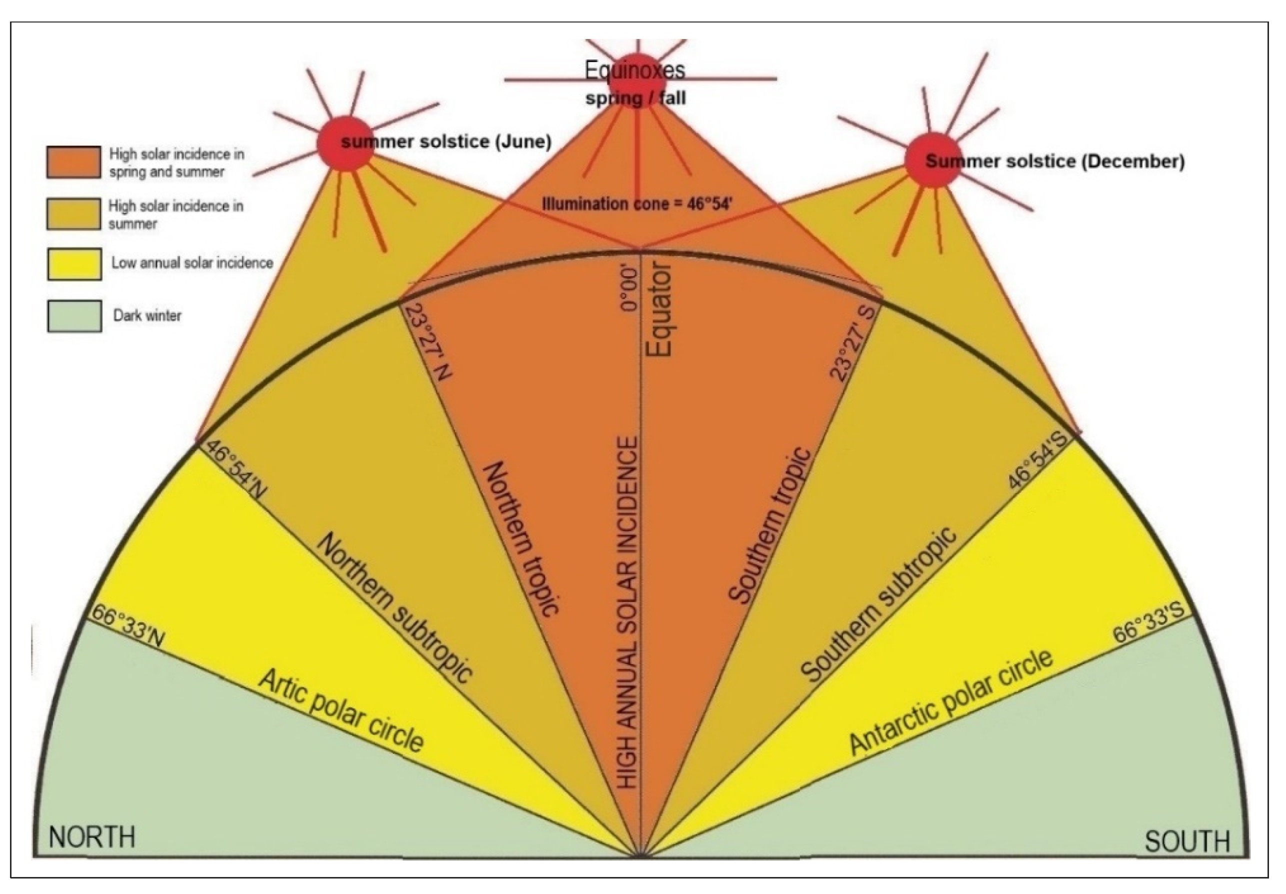
Figure 2.
Methodological approach.
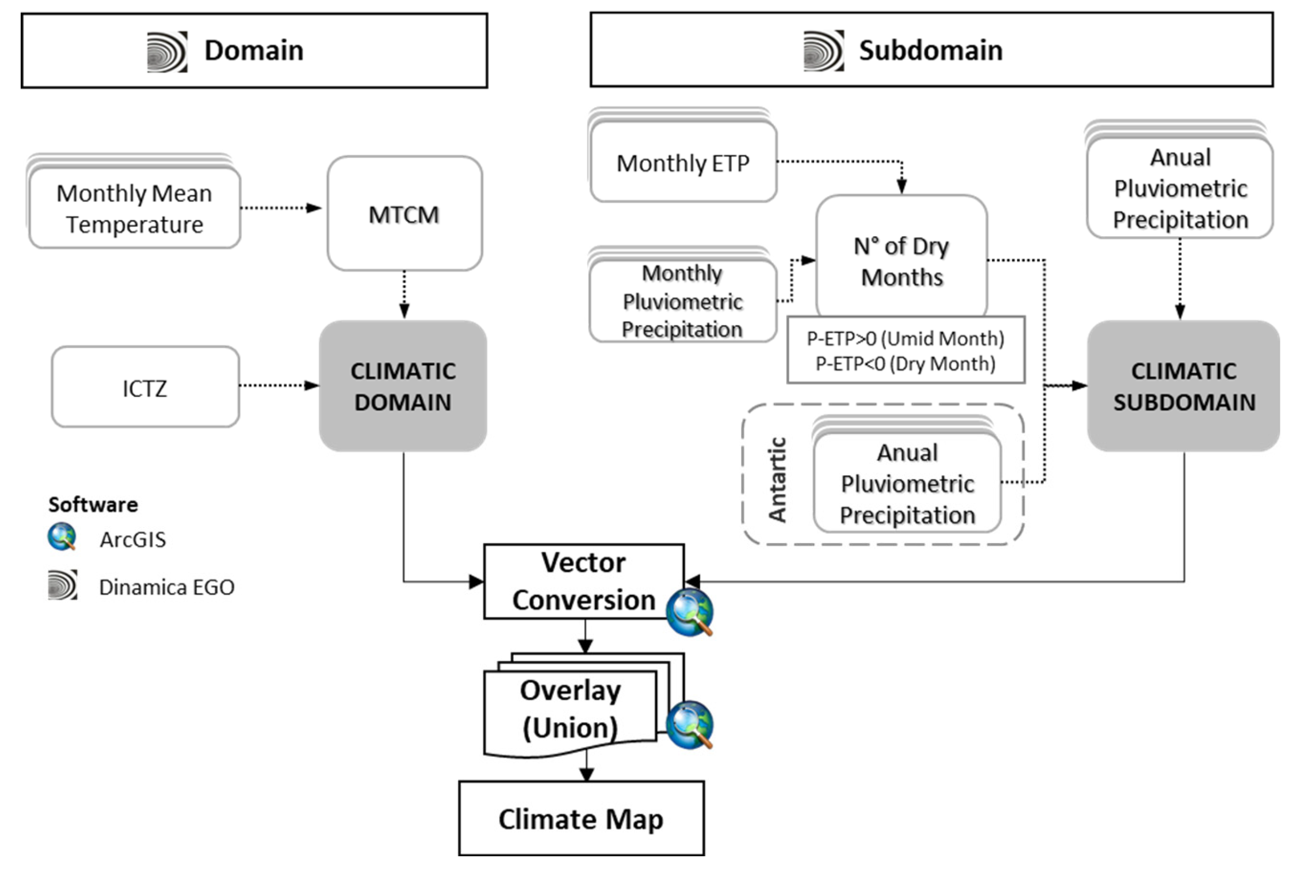
Figure 3.
Coding scheme employed to distinguish climate units in the mapped representation.
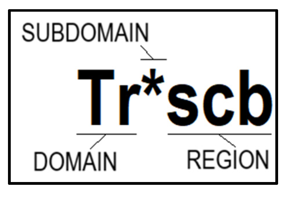
Figure 4.
Earth climatic zones. Novais and Machado (2023).
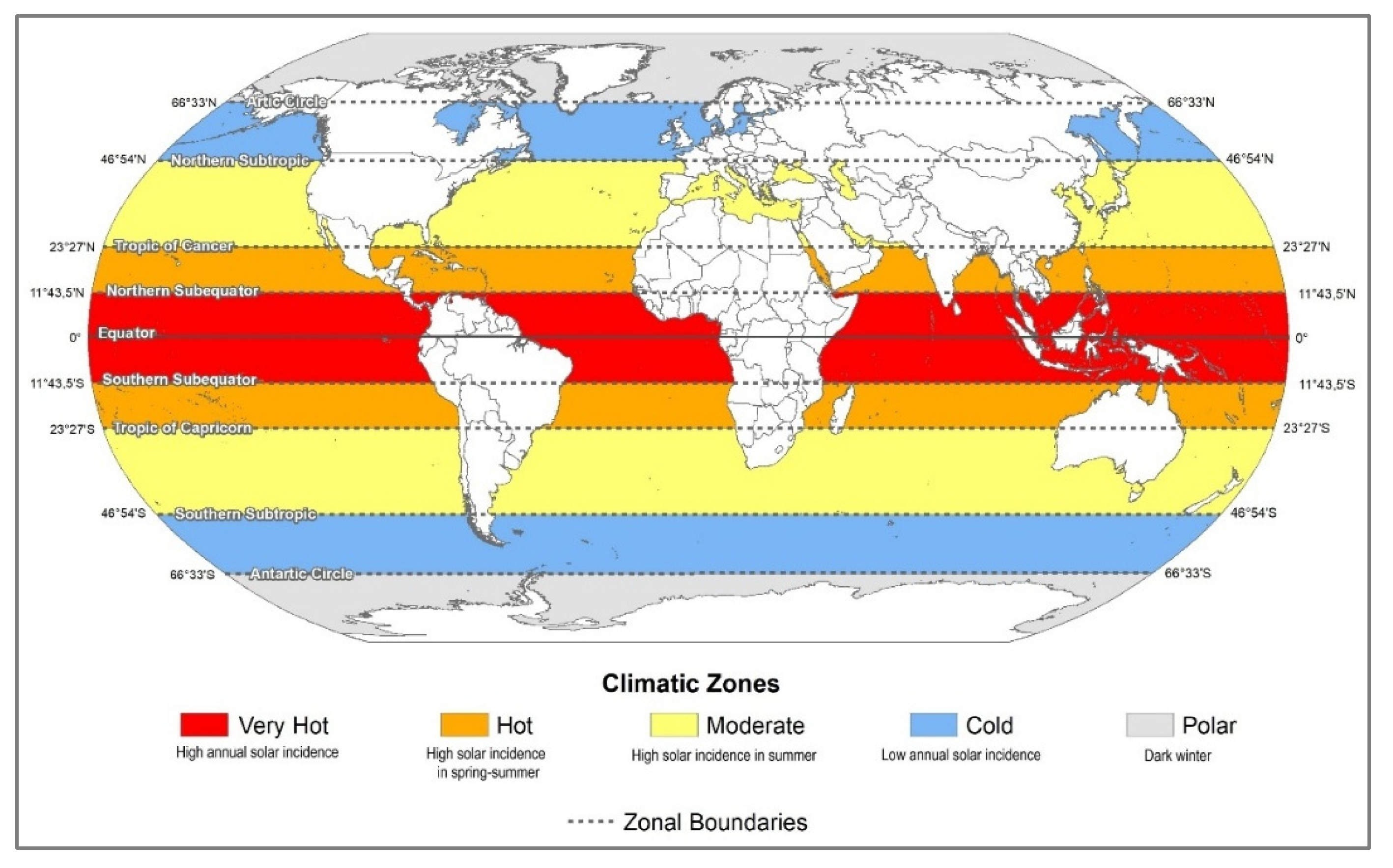
Figure 5.
Global zonal climates. Novais and Machado (2023).
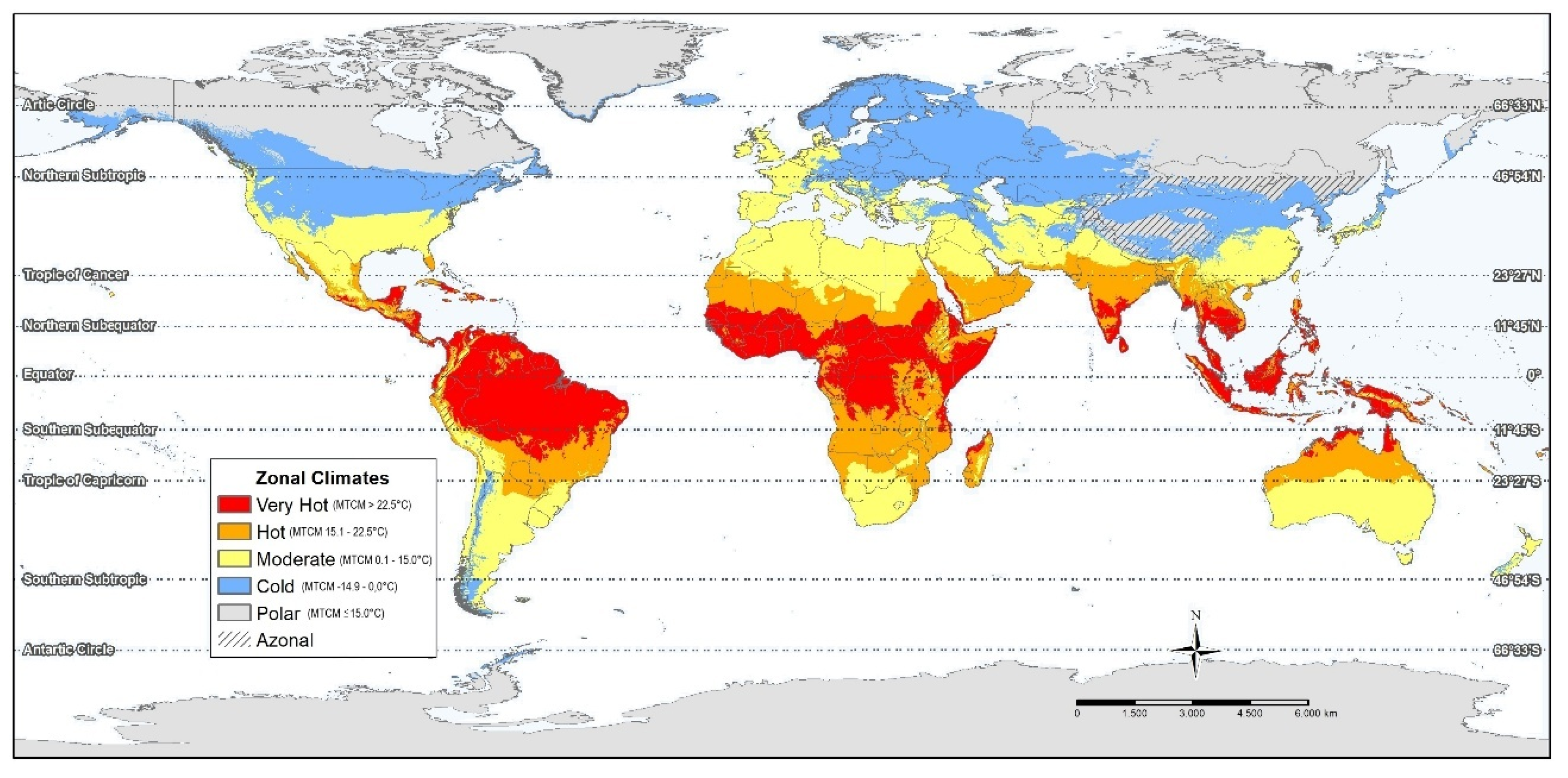
Figure 6.
Novais global climate classification map (climatic domains and subdomains).
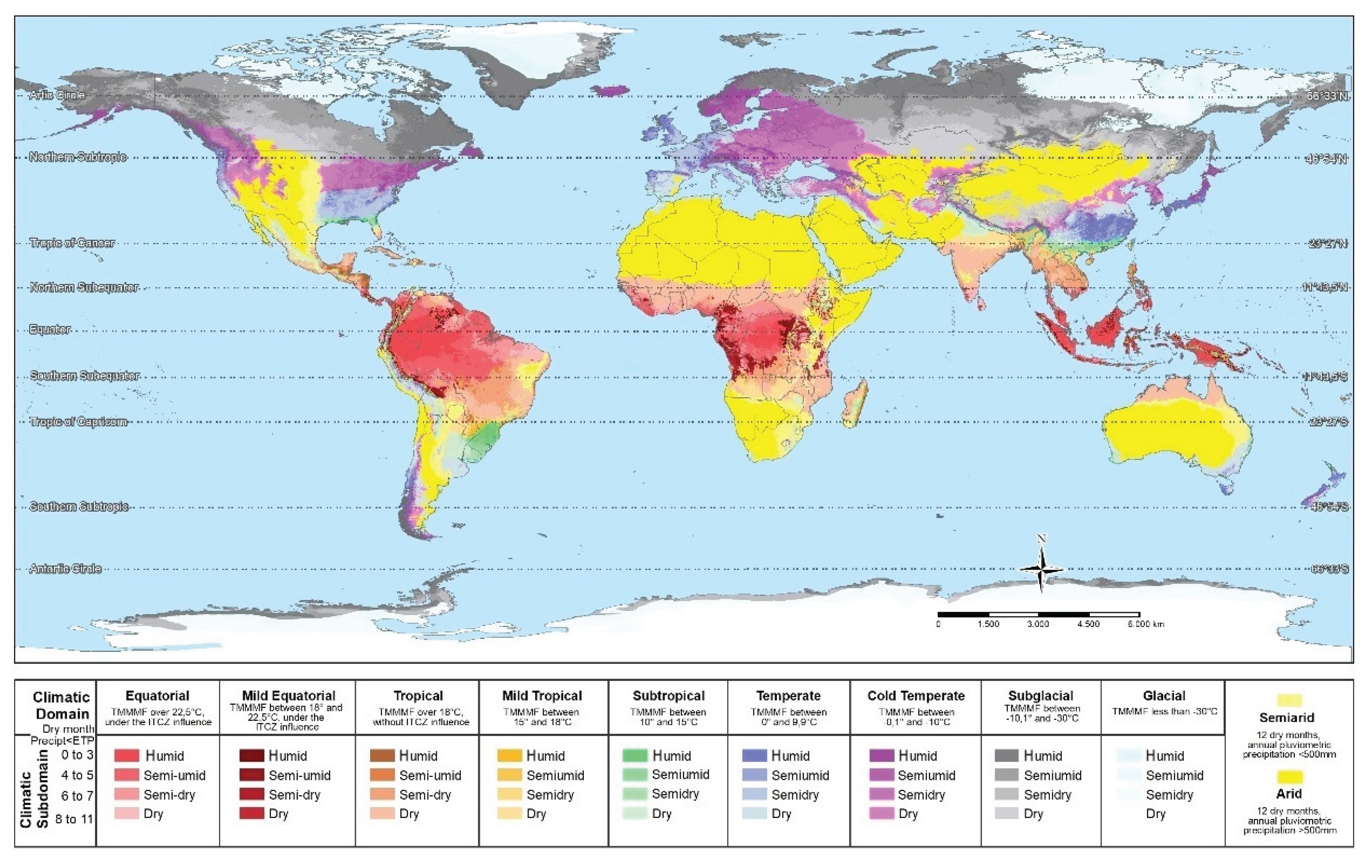
Table 1.
Scales hierarchy in Novais’s Climate Classification System.
| Order of Magnitude | Scales | Hierarchies | Spatial Examples | Surface Units | Cartographic Scale | Organizational Factors | Criteria |
| Upper level of climatic scale | Zonal | Climatic Zone | Continents, oceans | Millions of km² | 1:10,000,000 to 1:100,000,000 | Latitude | Solar incidence (Sun altitude) |
| Zonal Climate | Continents, major landform units | Tens to thousands of km² | 1:100,000 to 1:10,000,000 | Atmospheric action centers, regional geographic factors | Mean Temperature of the Coldest month (MTCM) | ||
| Regional | Climatic Domain | Countries, morphoclimatic domains, major landform units | Tens to thousands of km² | 1:100,000 to 1:5,000,000 | Secondary circulation, regional geographic factors | MTCM, Intertropical Convergence Zone (ITCZ), precipitation, dry months | |
| Climatic Subdomain | Major landform units and morphoclimatic domains | Tens to thousands of km² | 1:100,000 to 1:5,000,000 | Secondary circulation, regional geographic factors | Number of dry months (precipitation < potential evapotranspiration) | ||
| Climatic Region | Morphoclimatic domains, landform units | Tens to thousands of km² | 1:100,000 to 1:5,000,000 | Regional geographic factors | Continental location | ||
| Lower level of climatic scale | Sub regional |
Climatic Subregion | Landform units and major metropolises | Tens to thousands of km² | 1:100,000 to 1:1,000,000 | Geoecological integration, human activity | Geomorphological units |
| Mesoclimate | Massifs, mountains, plains, plateaus, depressions; metropolitan areas, big municipalities | Tens to hundreds of km² | 1:50,000 to 1:100,000 | Geoecological integration, human activity, urbanism | Third and fourth geomorphological taxa, meteorological stations | ||
| Local |
Topoclimate/ Local Climate |
Summit areas of mountains and plateaus, ridgelines, slopes, urban areas, parks | m² to tens of km² | 1:5,000 to 1:50,000 | Geoecological integration, human activity, urbanism, architecture | Fifth geomorphological taxon, instrumental measurement |
Table 2.
Climatic Zones of Novais Climate Classification System.
| Climatic Zone | Location | Solar radiation | Minimum Solar Altitude on the Horizon | Day/Night Variation |
|
Very Hot (Torrid) |
Between the subequators (±11°43’30”) | Maximum throughout the year; Sun at zenith twice | 54°49’30” | Up to 35 minutes |
| Hot | Between subequators and tropics (±23°27’) | High; Sun at zenith twice and once over the tropic | 43°06’ | Up to 1h35min |
| Moderate | Between tropics and subtropics (±46°54”) | High in summer; Sun never at zenith (except on the tropic) | 19°39’ | Up to 3h19min |
| Cold | Between subtropics and polar circles (±66°33’) | Low; cold surface for most of the year | 0° | Average of 7h30min |
| Polar | Between polar circles and the poles | Minimal; Absent during winter, but visible 24 hours a day in summer | Negative (darkness) | Ranges from 0h to 24h |
Table 3.
Climatic domains classification.
| Climatic Domain | MTCM (°C) / ITCZ | Dry Months / Annual Average Precipitation (AAP) |
| Equatorial (Eq) | > 22.5 + ITCZ | - |
| Mild Equatorial (EqM) | 18.1 to 22.5 + ITCZ | - |
| Tropical (Tr) | > 18.0 + without ITCZ | - |
| Mild Tropical (TrM) | 15.1 to 18.0 | - |
| Subtropical (St) | 10.1 to 15.0 | - |
| Temperate (Te) | 0.1 to 10.0 | - |
| Cold Temperate (TeC) | −9.9 to 0.0 | - |
| Subglacial (Sg) | −29.9 to −10.0 | - |
| Glacial (Gl) | ≤ −30.0 | - |
| Semiarid (SA) | - | 12 dry months + AAP > 500 mm |
| Arid (Ar) | - | 12 dry months + AAP < 500 mm |
Table 4.
Climatic subdomains (domains) classification.
| Climatic Subdomain / Climatic Domain | Number of Dry Months | Annual Average Precipitation |
| Humid | Up to 3 | - |
| Semihumid | 4 to 5 | - |
| Semidry | 6 to 7 | - |
| Dry | 8 to 11 | - |
| Semiarid | 12 | > 500 mm |
| Arid | 12 | < 500 mm |
Table 7.
Comparison between Köppen’s climatic groups and the thermal–hydrological domains and subdomains of Novais.
Table 7.
Comparison between Köppen’s climatic groups and the thermal–hydrological domains and subdomains of Novais.
| Köppen Climatic Group | Thermal / Hydrological Thresholds (Köppen) | Corresponding Novais Domains | Corresponding Novais Subdomains | Notes |
| A – Tropical | Tmin (coldest month) ≥ 18 °C | Equatorial, Mild Equatorial, Tropical, Mild Tropical | Humid (“), Semihumid (‘), Semidry (*), Dry (**) | Novais subdivides Köppen’s broad tropical belt into four thermal bands based on MTCM and ITCZ influence. |
| Af – Tropical Rainforest | No dry month; Pmin ≥ 60 mm | Equatorial / Tropical (humid) | (“) humid | Strong match with Novais’s humid tropical units, especially in Amazonia and Central Africa. |
| Am – Monsoon | Short dry season | Tropical / Mild Tropical | (‘) semihumid | Corresponds to monsoon-influenced tropical units in S. Asia, N. Australia, NE Brazil margins. |
| Aw/As – Savanna | Dry winter/summer | Tropical / Mild Tropical | (*) semidry or (**) dry (depending on duration) | Novais separates savannas by number of dry months (hydrological threshold), not only season. |
| B – Dry (Arid/Semiarid) | Pann < Pthreshold (temperature-dependent) | Arid, Semiarid | Dry (**) only | Novais uses fixed rainfall limit (500 mm) + 12 dry months → clearer physiological meaning than Bs/Bw. |
| BSh – Hot Steppe | Semiarid | Semiarid | Dry (**) | Spatial agreement is strong (Novais 2023a). |
| BWh – Hot Desert | Arid | Arid | Dry (**) | Matches major desert regions: Sahara, Atacama, Arabia, Australia. |
| C – Temperate / Mesothermal | –3 °C < Tmin < 18 °C | Mild Tropical, Subtropical, Temperate | All subdomains possible | Köppen’s broad interval is subdivided into 4 thermal domains in Novais. |
| Cfa/Cfb – Humid Temperate | No dry season | Subtropical / Temperate (humid) | (“) humid | Strong overlap with Western Europe, SE South America. |
| Csa/Csb – Mediterranean | Dry summer | Subtropical / Temperate (semidry) | (‘) semihumid or (*) semidry | Novais discriminates Mediterranean types by number of dry months, not season only. |
| D – Cold Continental | Tmin < –3 °C; Tmax > 10 °C | Temperate, Cold Temperate, Subglacial | All subdomains possible | Köppen’s D-group spans several Novais thermal domains depending on winter temperature. |
| Dfb/Dfc – Boreal | Cold winter, humid | Cold Temperate | (“) to (*) | Matches boreal regions of Canada, Russia, Scandinavia. |
| E – Polar | Tmax (warmest month) < 10 °C | Subglacial, Glacial | Dry (**) | Novais refines Köppen’s ET/EF with specific lower thermal bands (–10 to –30 °C; ≤ –30 °C). |
| ET – Tundra | 0 ≤ Tmax < 10 °C | Subglacial (upper limit) | Dry (**) | Partial correspondence with cold-temperate/subglacial depending on thermal regime. |
| EF – Ice Cap | Tmax < 0 °C | Glacial | Dry (**) | Strong match with Novais’s glacial domain. |
Table 8.
Comparison between Strahler’s dynamic climate classification and the Novais climatic system.
Table 8.
Comparison between Strahler’s dynamic climate classification and the Novais climatic system.
| Aspect | Strahler (1951, 1989) | Novais (2019–2023) | Notes / Key Differences |
| Primary Basis | Atmospheric circulation belts (Hadley, Ferrel, Polar cells) | Thermal domains + hydrological subdomains + dynamic/geomorphic controls | Novais integrates more environmental variables. |
| Core Objective | Explain global zonal climate structure using circulation dynamics | Produce high-resolution global climate mapping with hierarchical detail | Novais focuses on spatial precision, not only zonal processes. |
| Treatment of Latitude | Strict latitudinal belts: tropical, subtropical, midlatitude, polar | Latitude interacts with thermal thresholds and ITCZ influence | Novais refines subtropical–tropical and equatorial boundaries. |
| Thermal Criteria | Broad zonal temperature character (no fixed thresholds) | Fixed thermal thresholds for 10 domains (e.g., >22.5 ºC; 15–18 ºC; –10 to –30 ºC) | Köppen-like precision, but more detailed. |
| Hydrological Criteria | Does not use dry-month counts or ETp | Subdomains defined by ETp and number of dry months (0–12) | Novais integrates Thornthwaite’s water balance. |
| Use of Precipitation Seasonality | Implicit (via circulation belts) | Explicit, via dry-month rules and ETp–P balance | Novais provides physiologically meaningful hydrological limits. |
| Role of Relief / Topography | Not included (Strahler assumes macro-zonal control) | Central component: relief modifies temperature, ETp, precipitation and defines many units | Key conceptual innovation of Novais. |
| Dryland Identification | Zonal hot-desert zones | Fixed thresholds: <500 mm and 12 dry months (arid) | More objective than circulation-only approach. |
Table 9.
Comparison between the Thornthwaite & Mather climate classification and the Novais climatic system.
Table 9.
Comparison between the Thornthwaite & Mather climate classification and the Novais climatic system.
| Aspect | Thornthwaite & Mather (1955) | Novais (2019–2023) | Key Notes |
| Conceptual Basis | Climatological water balance (P – ETp) | Thermal domains + hydrological subdomains + dynamic & geomorphic factors | Novais builds on Thornthwaite’s hydrological logic and expands it. |
| Primary Variables | Precipitation (P), Potential Evapotranspiration (ETp) | Temperature thresholds, dry months, ETp–P balance, relief, ITCZ influence | Novais integrates more variables and regional context. |
| Hydrological Criteria | Central element: water balance defines humidity/aridity classes | Dry-month thresholds + ETp–P balance define subdomains | Shared foundation, but Novais adds seasonal detail. |
| Thermal Criteria | Uses thermal efficiency index (heat index) | Fixed thermal bands for 10 domains | Novais replaces Thornthwaite’s heat index with explicit thresholds. |
| Seasonality | Recognizes seasonal water surplus/deficit | Explicitly counts dry months (0–12) | Novais operationalizes seasonality more directly. |
| Role of Relief | Not incorporated | Central element (controls local temperature, ETp, precipitation) | Major difference between the systems. |
| Geographic Resolution | Broad functional categories | High detail across 5 hierarchies | Novais provides finer spatial discrimination. |
Disclaimer/Publisher’s Note: The statements, opinions and data contained in all publications are solely those of the individual author(s) and contributor(s) and not of MDPI and/or the editor(s). MDPI and/or the editor(s) disclaim responsibility for any injury to people or property resulting from any ideas, methods, instructions or products referred to in the content. |
© 2026 by the authors. Licensee MDPI, Basel, Switzerland. This article is an open access article distributed under the terms and conditions of the Creative Commons Attribution (CC BY) license (http://creativecommons.org/licenses/by/4.0/).
Copyright: This open access article is published under a Creative Commons CC BY 4.0 license, which permit the free download, distribution, and reuse, provided that the author and preprint are cited in any reuse.


