Submitted:
31 January 2026
Posted:
02 February 2026
You are already at the latest version
Abstract
We study holonomy-induced deviations arising from Levi-Civita parallel transport on Calabi-Yau manifolds of complex dimensions one through four. Using the Ricci-flat Kähler structure and the associated SU(n) holonomy reduction, we develop a unified framework for deviation operators that applies uniformly across dimensions. General expressions are formulated in terms of path-ordered transport, curvature endomorphisms, and non-Abelian Stokes techniques, clarifying how nontrivial holonomy effects persist despite vanishing Ricci curvature. A dimension-by-dimension analysis is presented, covering elliptic curves, K3 and abelian surfaces, Calabi-Yau threefolds, and Calabi-Yau fourfolds. We identify which holonomy contributions are suppressed by type constraints in Kähler geometry, which arise only at higher order, and how these features depend on the complex dimension. The paper is intended both as a reference for explicit holonomy and deviation computations and as a bridge to applications involving geometric phases and compactification effects.
Keywords:
SU(n) holonomy deviation operators
; non-abelian parallel transport
; Weyl-curvature--induced holonomy
MSC: Primary: 53C44 (Geometric evolution equations; Ricci-flat and special holonomy metrics), 53C55 (Complex differential geometry; Kähler and Calabi–Yau geometry), 53C80 (Applications of differential geometry to physics); Secondary: 83E30 (String and supergravity theory; compactifications), 53B21 (Methods of Riemannian geometry), 81T30 (String theory and branes), 14J32 (Calabi–Yau manifolds and higher-dimensional varieties), 32Q25 (Special Kähler metrics; Calabi–Yau metrics).
Reader Guide (How to Read This Paper)
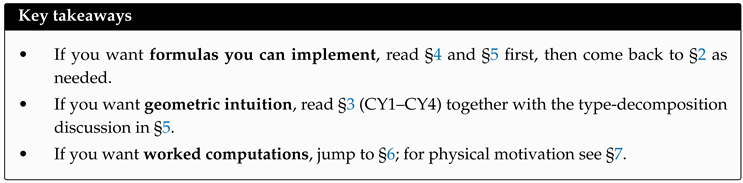
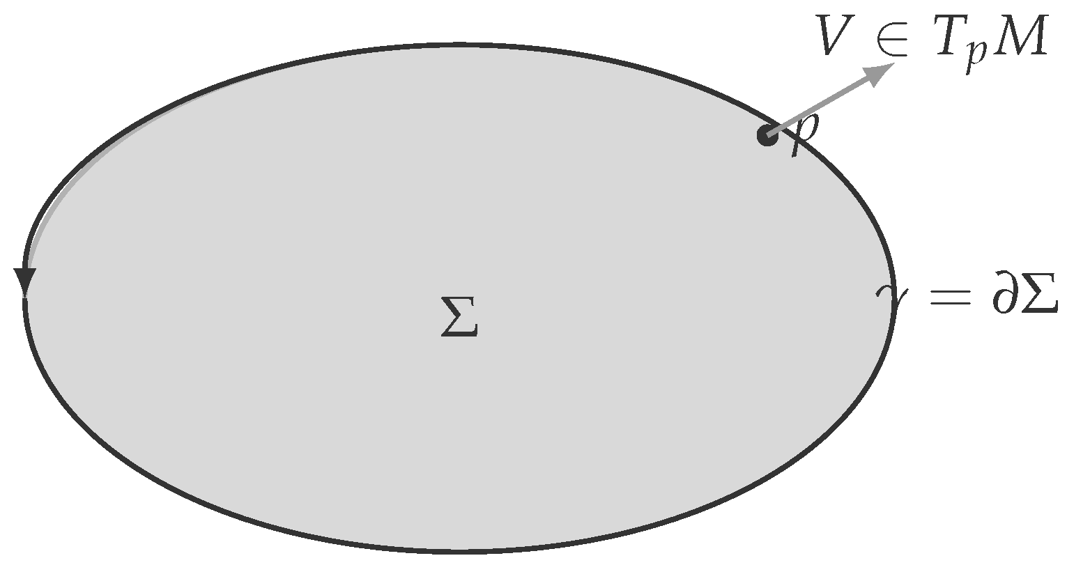
Figure 1.
Holonomy as loop memory: the Levi–Civita connection ∇ and curvature R induce a loop transformation , and the deviation operator is .
Figure 1.
Holonomy as loop memory: the Levi–Civita connection ∇ and curvature R induce a loop transformation , and the deviation operator is .
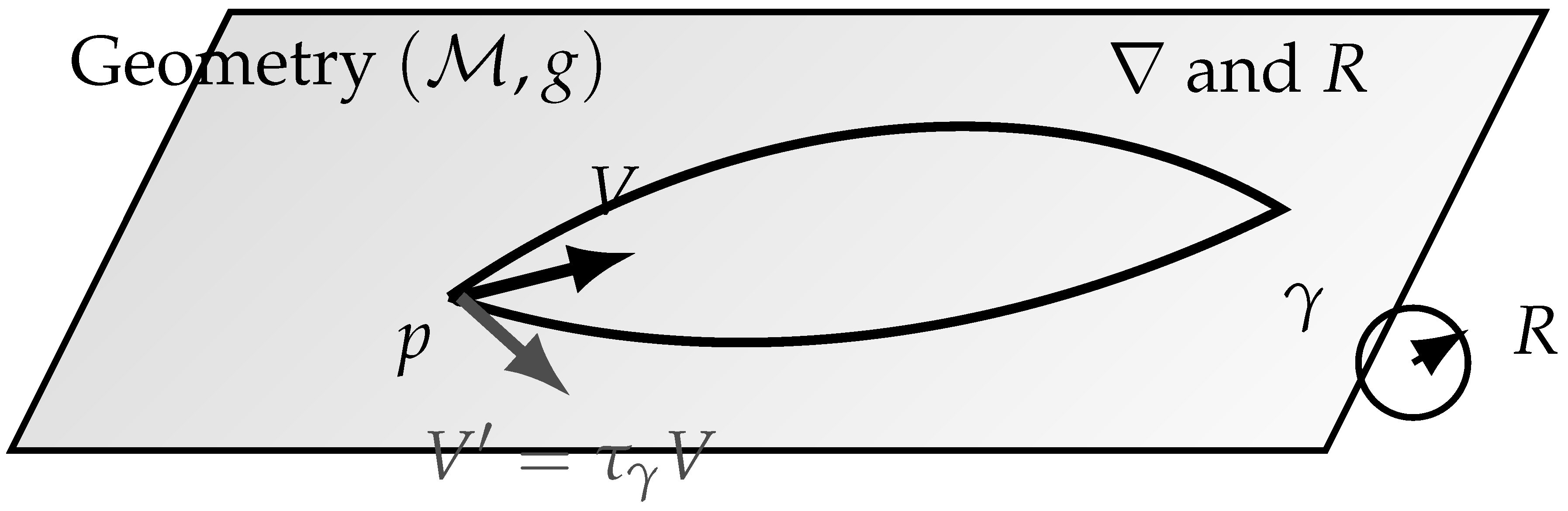

Table 1.
Comparison of Calabi–Yau manifolds across CY1–CY4.
| Dimension | Typical examples | Levi–Civita holonomy | Physics motivation |
| CY1 () | elliptic curve | trivial () | worldsheet tori, flat bundles |
| CY2 () | K3; abelian surface | (K3), trivial (torus) | string dualities, BPS states |
| CY3 () | quintic; toric hypersurfaces | typically | compactification, mirror symmetry |
| CY4 () | elliptic/toric CY4 | typically | F-theory, flux vacua |
1. Introduction and Overview
1.1. Historical Context and Motivation
The study of parallel transport and holonomy represents one of the most profound intersections between differential geometry and theoretical physics. Since Levi-Civita’s introduction of the concept of parallel displacement in 1917, the mathematical theory of connections and holonomy has evolved into a rich field with applications spanning general relativity, gauge theory, and string theory. The central question—how a geometric space "remembers" the path along which a vector has been transported—encapsulates fundamental aspects of curvature, topology, and geometric phases.
Calabi-Yau manifolds, first conjectured by Calabi in 1954 and proven to exist by Yau in 1978 [3], have emerged as cornerstone objects in modern theoretical physics, particularly in string theory compactification scenarios [5,23]. These Ricci-flat Kähler spaces with SU(n) holonomy provide natural candidates for the extra dimensions required by superstring theories. Their mathematical elegance—characterized by vanishing first Chern class, existence of covariantly constant spinors, and rich moduli spaces—makes them ideal laboratories for exploring deep geometric phenomena.
The specific problem of computing exact deviations during Ricci transport over Calabi-Yau manifolds sits at the confluence of several important research directions: (1) the classical theory of holonomy and parallel transport in Riemannian geometry [1,2], (2) the specialized geometry of Kähler and Calabi-Yau spaces [3,25], (3) physical applications in string theory and quantum field theory [5,23], and (4) mathematical developments in geometric analysis and complex differential geometry [11,43]. Recent preprint studies have further expanded this landscape [4].
1.2. Fundamental Questions and Objectives
This paper addresses the following fundamental questions:
- 1.
- How can we formulate and compute the exact deviation between initial and final vectors after Ricci transport along closed loops in Calabi-Yau manifolds?
- 2.
- What simplifications occur due to Ricci-flatness and SU(n) holonomy?
- 3.
- How do the complex structure and Kähler structure influence the deviation?
- 4.
- What are the physical implications for string compactification and geometric phases?
- 5.
- How can we connect local curvature computations to global topological invariants?
Our primary objectives include:
- Developing a comprehensive mathematical framework for analyzing Ricci transport on Calabi-Yau manifolds
- Deriving multiple representations of the deviation tensor (series, exponential, integral forms)
- Establishing connections between deviation tensors and topological invariants
- Providing explicit computational methods and examples
- Exploring physical applications in theoretical physics
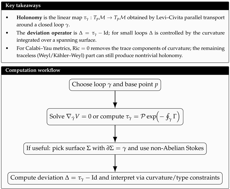
Table 2.
Roadmap: how to use this paper depending on your goal.
| Section | Reader goal / what you get |
|---|---|
| §2 | Core definitions (connections, curvature, holonomy, Kähler/CY structure) + the formulas used later. |
| §3 | CY1–CY4 “dimension ladder” with what is (im)possible for holonomy deviation in each case. |
| §4 | General deviation/holonomy machinery: infinitesimal loops, Wilson loops, Stokes, series/Magnus expansions. |
| §5 | CY-specific simplifications: type decomposition, traceless curvature, SU(n) constraints on . |
| §6 | Worked examples and computational recipes (analytic where possible; numerical where necessary). |
| §7 | Physical interpretations (Berry phases, compactification, moduli-space loops, etc.). |
1.3. Structure of the Paper
This paper is organized to progressively develop a general framework for Levi–Civita holonomy deviation on Calabi–Yau manifolds and to specialize it across dimensions, examples, and applications.
Section 2 establishes the mathematical foundations required throughout the paper. We review Riemannian geometry, Levi–Civita parallel transport, curvature tensors, holonomy groups, and the basic structures of Kähler and Calabi–Yau manifolds, fixing notation and conventions used later. Technical material concerning the decomposition of curvature on Ricci-flat Kähler manifolds and the reduction of curvature endomorphisms to is deferred to Appendix A.
Section 3 provides a dimension-by-dimension survey of Calabi–Yau manifolds of complex dimensions one through four (CY1–CY4). For each dimension we summarize representative constructions, moduli, and the geometric mechanisms that constrain which holonomy and deviation effects can arise. Special attention is paid to symmetry-driven cancellations, particularly in the CY2 (hyperkähler) case. A detailed discussion of these hyperkähler symmetry cancellations and their impact on the deviation operator is presented separately in Appendix C.
Section 4 develops the general theory of holonomy deviation operators. Beginning with infinitesimal loops, we derive the leading curvature-controlled deviation and its formulation in terms of area bivectors. We then extend the analysis to finite loops using path-ordered exponentials and non-Abelian Stokes-type representations, and we discuss series expansions, commutator effects, and convergence issues. Higher-order resummation techniques, including the Magnus expansion for Levi–Civita holonomy, are collected in Appendix B in order to keep the main text focused on geometric structure and interpretation.
Section 5 specializes the general deviation framework to Calabi–Yau geometry. Exploiting Ricci-flatness, Kähler type decomposition, and holonomy reduction, we derive simplified and dimension-dependent expressions for the deviation operator. We identify which curvature components control nontrivial holonomy despite vanishing Ricci curvature and clarify which potential contributions are forbidden by type or representation-theoretic constraints.
Section 6 presents explicit computations and worked examples on representative Calabi–Yau spaces, including flat tori, K3 surfaces, and Calabi–Yau threefolds. These examples illustrate how the general formulas developed earlier may be implemented analytically in high-symmetry settings and numerically in more general situations.
Section 7 discusses physical and geometric applications of holonomy-induced deviation, including geometric phases, string compactifications, and moduli-space dynamics, where Levi–Civita transport around nontrivial loops plays a central role.
Section 8 reviews recent developments and related preprint literature on Ricci-flat transport, holonomy, and curvature-induced effects in Calabi–Yau and special-holonomy settings, placing the present work in context.
Finally, Section 9 summarizes the main results of the paper and outlines directions for future investigation.
Appendices.
Appendix A collects the curvature decomposition formulas for Ricci-flat Kähler manifolds and the associated constraints used throughout Section 4 and Section 5. Appendix B presents the Magnus expansion and related resummation techniques for Levi–Civita holonomy, complementing the series expansions discussed in Section 4. Appendix C analyzes hyperkähler symmetry and explicit cancellation mechanisms for holonomy deviation on CY2 manifolds, providing technical support for the claims made in Section 3.
1.4. Scope and Roadmap: CY1–CY4
The scope of this expanded version is explicitly dimension-spanning: we treat Calabi–Yau manifolds of complex dimension in a unified framework, while also isolating the features that are genuinely dimension-dependent.
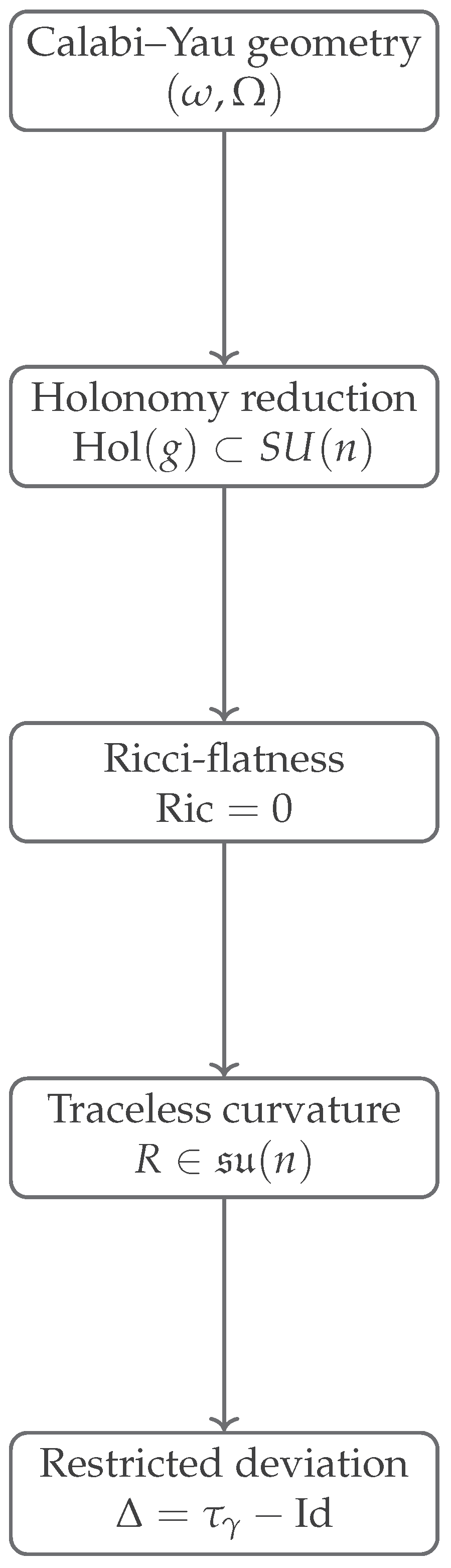
At a conceptual level, the common core is the following chain:
However, the representation-theoretic content of , the available calibrated submanifolds, and the moduli-space geometry all vary significantly with n. We therefore interleave the general deviation/holonomy derivations with dimension-specific discussions and examples.
1.5. Notation and Conventions
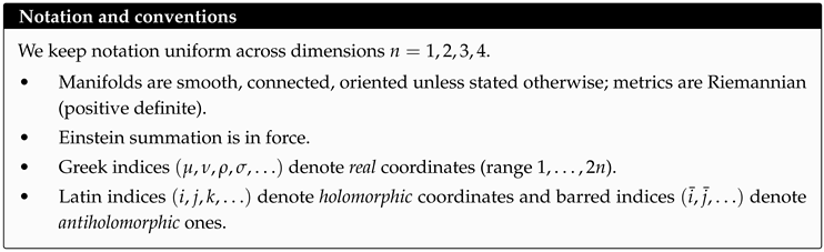
Figure 2.
Conceptual flow from geometry to deviation under Levi–Civita parallel transport.
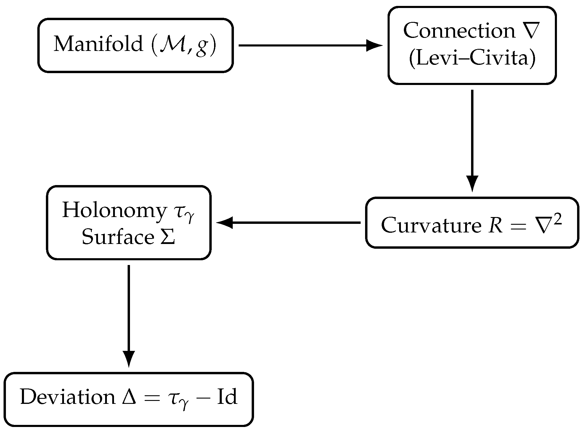
Table 3.
Frequently used notation (quick lookup).
| Symbol | Meaning (default in this paper) |
|---|---|
| ∇ | Levi–Civita connection of g; also written via Christoffel symbols . |
| Riemann curvature tensor (sign convention fixed in §2); . | |
| , R | Ricci tensor and scalar curvature. For Calabi–Yau: (and hence ). |
| Levi–Civita holonomy group of g (at a point; groups are conjugate on connected manifolds). | |
| , | Loop and a spanning surface with . |
| Parallel transport map around (holonomy element). | |
| Deviation operator: . | |
| , | Kähler form and covariantly constant holomorphic volume form on a Calabi–Yau n-fold. |
Curvature sign convention. In coordinates we use
so that infinitesimal holonomy around an area element is controlled by as in §4.
2. Mathematical Preliminaries
Table 4.
Core geometric ingredients and where they feed into holonomy/deviation computations.
| Object | What it does / why it appears in this paper |
|---|---|
| ∇ (Levi–Civita) | Defines parallel transport; metric-compatible and torsion-free. |
| Parallel transport ODE | ; solution defines . |
| R (curvature) | Infinitesimal failure of path-independence; generates the holonomy algebra (Ambrose–Singer). |
| Kähler structure | Enforces type constraints (only -type curvature components survive). |
| Calabi–Yau structure | Implies and ; curvature is traceless in the relevant sense. |
In addition to the classical literature on holonomy, curvature, and Calabi–Yau geometry, there exists a body of complementary work that addresses related algebraic, cohomological, and operator-theoretic structures relevant to geometric transport problems. In particular, enumerative norms arising from quantum cohomological connectivity and Gromov–Witten theory have been studied in a rigorous preprint framework, highlighting how global enumerative data can be constrained by cohomological and topological input [17]. Related topological aspects appear in analyses of the Atiyah–Hirzebruch spectral sequence for twisted K–theory, where integral cohomology classes and duality considerations play a central role in organizing higher-order topological information [8]. From a more algebraic perspective, operator-algebraic approaches to commutative measurable structures on compact Hausdorff spaces have been developed using von Neumann and AW*–algebra techniques, providing abstract tools that parallel functional-analytic methods employed in geometric quantization and deformation theory [9]. While these works address distinct mathematical questions, they complement the present study by situating curvature-induced transport and holonomy within a broader algebraic and cohomological landscape.
2.1. Riemannian Geometry Fundamentals
2.1.1. Manifolds, Metrics, and Connections
Let be a smooth manifold of dimension m. A Riemannian metric g is a smooth, symmetric, positive-definite -tensor field on . The pair is called a Riemannian manifold. The metric induces an inner product on each tangent space :
Definition 1
(Levi-Civita Connection). The Levi-Civita connection ∇ is the unique torsion-free, metric-compatible affine connection on a Riemannian manifold. In local coordinates, the connection coefficients (Christoffel symbols) are given by:
2.1.2. Parallel Transport and Geodesics
Given a curve with tangent vector , a vector field along is said to be parallel transported if:
Geodesics are curves that parallel transport their own tangent vectors:
2.1.3. Curvature Tensors
The Riemann curvature tensor measures the failure of parallel transport around infinitesimal loops. For a vector transported around an infinitesimal parallelogram spanned by vectors and , the change is given by:
The Riemann tensor satisfies the following symmetries:
The Ricci tensor and scalar curvature are contractions:
The Weyl tensor (conformal curvature tensor) in dimensions is:
The Weyl tensor vanishes identically for and captures the traceless part of the curvature [6,7,37].
2.2. Kähler Geometry
2.2.1. Complex Manifolds and Hermitian Metrics
A complex manifold of complex dimension n has local holomorphic coordinates () and transition functions that are holomorphic. The complex structure is represented by an endomorphism satisfying .
A Hermitian metric h on a complex manifold is a Riemannian metric that is compatible with the complex structure:
In local coordinates, , with .
2.2.2. Kähler Condition
A Hermitian metric is Kähler if the associated Kähler form
is closed: . Equivalently, in local coordinates:
For Kähler metrics, the Christoffel symbols have special properties:
and all mixed components vanish: .
2.2.3. Kähler Curvature
The Riemann tensor for a Kähler manifold has additional symmetries:
The only non-vanishing components (up to complex conjugation and symmetry) are and its permutations.
The Ricci tensor on a Kähler manifold is given by:
The Ricci form is defined as:
2.3. Calabi-Yau Manifolds
2.3.1. Definition and Basic Properties
Definition 2
(Calabi-Yau Manifold). A Calabi-Yau manifold is a compact Kähler manifold with vanishing first Chern class .
By Yau’s proof of the Calabi conjecture [3], such manifolds admit Ricci-flat Kähler metrics. In fact, given any Kähler class , there exists a unique Ricci-flat Kähler metric in that class.
2.3.2. Holonomy Groups
For a Riemannian manifold , the holonomy group at a point p is the group of linear transformations on induced by parallel transport around closed loops based at p.
For a Calabi-Yau manifold of complex dimension n:
This has important consequences:
- Existence of a covariantly constant holomorphic -form
- Existence of covariantly constant spinors (important for supersymmetry)
- Ricci-flatness:
2.3.3. Covariantly Constant Forms
On a Calabi-Yau n-fold, there exists a nowhere vanishing holomorphic n-form satisfying:
In local coordinates, , where is a non-vanishing holomorphic function.
The Kähler form and are related by the normalization condition:
2.3.4. Moduli Spaces
Calabi-Yau manifolds come in continuous families. The moduli space has two branches:
- Complex Structure Moduli Space: Deformations of the complex structure preserving the Calabi-Yau condition
- Kähler Moduli Space: Deformations of the Kähler class while maintaining Ricci-flatness
For a Calabi-Yau n-fold, the Hodge numbers determine the dimensions of these moduli spaces [13,15,48].
2.3.5. Dimension-by-Dimension Taxonomy (CY1–CY4)
Although the definition of a Calabi–Yau manifold is uniform, the geometry and available constructions depend strongly on the complex dimension.
Table 5.
CY1–CY4: what changes with complex dimension and how it impacts holonomy deviation.
| CY | Key geometry | Levi–Civita holonomy | What to expect for |
|---|---|---|---|
| CY1 | flat complex torus / elliptic curve | trivial | for contractible loops (tangent bundle). |
| CY2 | K3 (hyperkähler) vs abelian surface (flat) | or trivial | strong symmetry/type cancellations; useful decomposition via . |
| CY3 | rich moduli + calibrated geometry | typically | first dimension where generic loops give nontrivial with genuine CY constraints. |
| CY4 | elliptic fibrations common; richer middle cohomology | typically | more independent curvature components; coupled Levi–Civita + gauge/flux holonomies often considered. |
CY1: Elliptic curves and complex tori.
A compact Calabi–Yau 1-fold is an elliptic curve equipped with its translation-invariant Kähler metric. The holonomy of the Levi–Civita connection is trivial (a subgroup of ), and the curvature vanishes for the flat metric, so Levi–Civita parallel transport around contractible loops yields no deviation. Nontrivial global effects arise instead from the non-simply-connected topology and from additional bundles/flat connections over E.
CY2: K3 surfaces and abelian surfaces.
In complex dimension , the principal simply-connected example is a K3 surface, whose Ricci-flat Kähler metrics are hyperkähler with holonomy . In contrast, an abelian surface admits a flat metric and hence trivial Levi–Civita holonomy. The hyperkähler structure on K3 provides strong algebraic constraints on curvature operators and allows additional decompositions of the deviation operator using the quaternionic triple of covariantly constant complex structures [25].
CY3: Threefold constructions and mirror symmetry.
In complex dimension , Calabi–Yau threefolds are central in string compactification and mirror symmetry. Standard constructions include complete intersections in projective/toric varieties (e.g., the quintic threefold) and toric hypersurfaces via reflexive polytopes [13]. Mirror symmetry predicts deep relationships among Hodge numbers, enumerative invariants, and periods; the Strominger–Yau–Zaslow (SYZ) picture interprets mirror symmetry in terms of special Lagrangian torus fibrations and duality, providing geometric input for the behavior of holonomy along families of cycles [26].
CY4: Fourfolds and higher-dimensional phenomena.
In complex dimension , Calabi–Yau fourfolds exhibit new features (e.g., richer middle cohomology and flux constraints in physical applications). Many CY4 examples arise as hypersurfaces/complete intersections in toric varieties and as elliptically fibered fourfolds. While the Levi–Civita holonomy still lies in , the representation theory and the possible calibrated submanifolds differ substantially from the case, which affects which loop/surface geometries can produce leading-order holonomy deviation.
2.4. Holonomy Theory and Ambrose-Singer Theorem
2.4.1. Holonomy Groups and Algebras
For a Riemannian manifold with connection ∇, the holonomy group at point p consists of all linear transformations induced by parallel transport around closed loops based at p.
The restricted holonomy group considers only null-homotopic loops. For a connected manifold, all holonomy groups are conjugate.
The holonomy algebra is the Lie algebra of the holonomy group.
2.4.2. Ambrose-Singer Theorem
Theorem 1
(Ambrose-Singer). The holonomy algebra is generated by the curvature endomorphisms and their parallel transports:
.
This theorem establishes a fundamental connection between local curvature and global holonomy. For a Levi-Civita connection on a Riemannian manifold, the curvature endomorphisms are skew-symmetric, so .
2.4.3. Berger’s Classification
Berger classified possible Riemannian holonomy groups. For irreducible, non-symmetric spaces, the possibilities are:
- : Generic Riemannian manifolds
- : Kähler manifolds
- : Calabi-Yau manifolds ()
- : Quaternionic-Kähler manifolds
- : Hyperkähler manifolds
- : 7-dimensional manifolds
- : 8-dimensional manifolds
2.5. Parallel Transport Formalism
2.5.1. Path-Ordered Exponentials
For a matrix-valued connection 1-form , parallel transport along a curve is given by the path-ordered exponential:
This satisfies the differential equation:
For the Levi-Civita connection, has components .
2.5.2. Non-Abelian Stokes Theorem
The non-Abelian Stokes theorem relates the path-ordered exponential around a closed loop to a surface-ordered exponential of the curvature:
where is the curvature 2-form, and is a surface bounded by [10].
For the Levi-Civita connection, corresponds to the Riemann curvature operator with components .
2.5.3. Series Expansion
The path-ordered exponential can be expanded as a series:
where .
Similarly, the deviation tensor can be expanded as:
| Symbol | Meaning |
| ∇ | Levi–Civita connection |
| Christoffel symbols | |
| Riemann curvature tensor | |
| Closed loop in the manifold | |
| Surface with boundary | |
| Parallel transport (holonomy) operator | |
| Deviation operator | |
| Kähler form | |
| Holomorphic volume form | |
| Levi–Civita holonomy group |
3. Calabi–Yau Manifolds Across Dimensions (CY1–CY4)
This section provides a dimension-by-dimension overview (CY1–CY4) with an emphasis on structures that directly affect Levi–Civita holonomy and the deviation operator derived later. We keep the presentation balanced: each dimension is treated both from the viewpoint of complex/Kähler geometry and from typical physics applications where parallel transport and geometric phases appear.
3.1. CY1: Elliptic Curves
A compact Calabi–Yau 1-fold is an elliptic curve for a lattice . Any translation-invariant metric is flat, hence the Levi–Civita curvature vanishes and the local (contractible-loop) holonomy is trivial. In particular, for a contractible loop and any tangent vector one has
so the deviation operator introduced in Section 4 vanishes identically at the level of the tangent bundle.
Nontrivial effects in CY1 are therefore typically (i) global/topological (coming from noncontractible loops, where one considers additional flat bundles), or (ii) gauge-theoretic (holonomy of an auxiliary connection rather than Levi–Civita). This distinction is conceptually important when comparing “geometric phase” discussions on elliptic curves with the genuine curvature-generated deviations on higher-dimensional Calabi–Yau manifolds [31].
3.2. CY2: K3 Surfaces and Abelian Surfaces
In complex dimension there are two prototypical behaviors:
- Abelian surfaces admit flat Kähler metrics, so Levi–Civita holonomy is trivial (as in CY1).
- K3 surfaces are simply connected and admit Ricci-flat Kähler metrics with holonomy ; in fact these metrics are hyperkähler.
For hyperkähler metrics, there exists a covariantly constant triple of complex structures satisfying the quaternionic relations. This leads to strong algebraic constraints on the curvature operator and its action on tensors, and it yields additional decompositions of the holonomy algebra and curvature endomorphisms [25,30].
From the holonomy-deviation viewpoint, the hyperkähler structure implies that many would-be “leading” contributions vanish for symmetry/type reasons; correspondingly, the first nontrivial deviation for certain families of loops can occur at higher order (cf. the type discussion in Section 5). Degenerations at large complex structure and their metric consequences also play a central role in CY2, particularly in relation to mirror-type phenomena for K3 [29].
Impact of hyperkähler symmetry.
The presence of a covariantly constant triple implies that curvature endomorphisms decompose into -valued components respecting the quaternionic structure. As a result, many potential contributions to the deviation operator cancel by symmetry, and certain loop geometries exhibit vanishing despite nonzero curvature [? ? ].
3.3. CY3: Threefolds, Toric Constructions, and Mirror Symmetry
Calabi–Yau threefolds (CY3) sit at the intersection of complex geometry and string compactification. Standard constructions include smooth hypersurfaces/complete intersections in projective space and hypersurfaces in toric varieties defined by reflexive polytopes [13,27].
For CY3, mirror symmetry provides powerful constraints on moduli-space geometry and on the behavior of families of cycles. In the Strominger–Yau–Zaslow (SYZ) picture, mirror symmetry is interpreted as T-duality along special Lagrangian torus fibrations, giving a geometric mechanism by which (families of) holonomy and parallel transport data vary across the moduli space [26].
From the perspective of this paper, CY3 is the first dimension where one simultaneously has:
- genuinely nontrivial Levi–Civita holonomy (typically full ),
- rich calibrated geometry (special Lagrangians, complex submanifolds), and
- physically meaningful moduli dynamics (e.g., geometric phases along moduli loops).
3.4. CY4: Fourfolds and F-theory Motivation
Calabi–Yau fourfolds (CY4) have holonomy contained in and display new features not present in CY3, particularly in the structure of middle cohomology and in typical fibration patterns (notably elliptic fibrations).
In physics, CY4 appear prominently in F-theory compactifications, where geometric data of elliptically fibered Calabi–Yau fourfolds encodes gauge sectors and flux choices; the geometry of the fibration and its singularities can induce nontrivial monodromy/transport phenomena on associated bundles over moduli spaces [33,47].
While our deviation operator is defined using the Levi–Civita connection on the Calabi–Yau itself, in CY4 applications one frequently studies coupled systems: Levi–Civita transport on the internal manifold together with transport in auxiliary (gauge/flux) bundles. This section isolates what is purely Levi–Civita and what arises from additional structures, so later applications can clearly separate geometric holonomy from gauge holonomy.
Table 7.
Comparison of Levi–Civita holonomy and deviation behavior across Calabi–Yau manifolds of different complex dimensions.
Table 7.
Comparison of Levi–Civita holonomy and deviation behavior across Calabi–Yau manifolds of different complex dimensions.
| CY dimension | Typical example | Holonomy | Deviation |
|---|---|---|---|
| CY1 () | Elliptic curve | Trivial | (flat) |
| CY2 () | K3 surface | Strong symmetry cancellations | |
| CY3 () | Quintic threefold | Generic nontrivial deviation | |
| CY4 () | Elliptic CY4 | Rich curvature-induced effects |
4. General Theory of Deviation Tensors
Figure 3.
Conceptual flow from Levi–Civita parallel transport around a closed loop to curvature-induced holonomy and the associated deviation operator .
Figure 3.
Conceptual flow from Levi–Civita parallel transport around a closed loop to curvature-induced holonomy and the associated deviation operator .
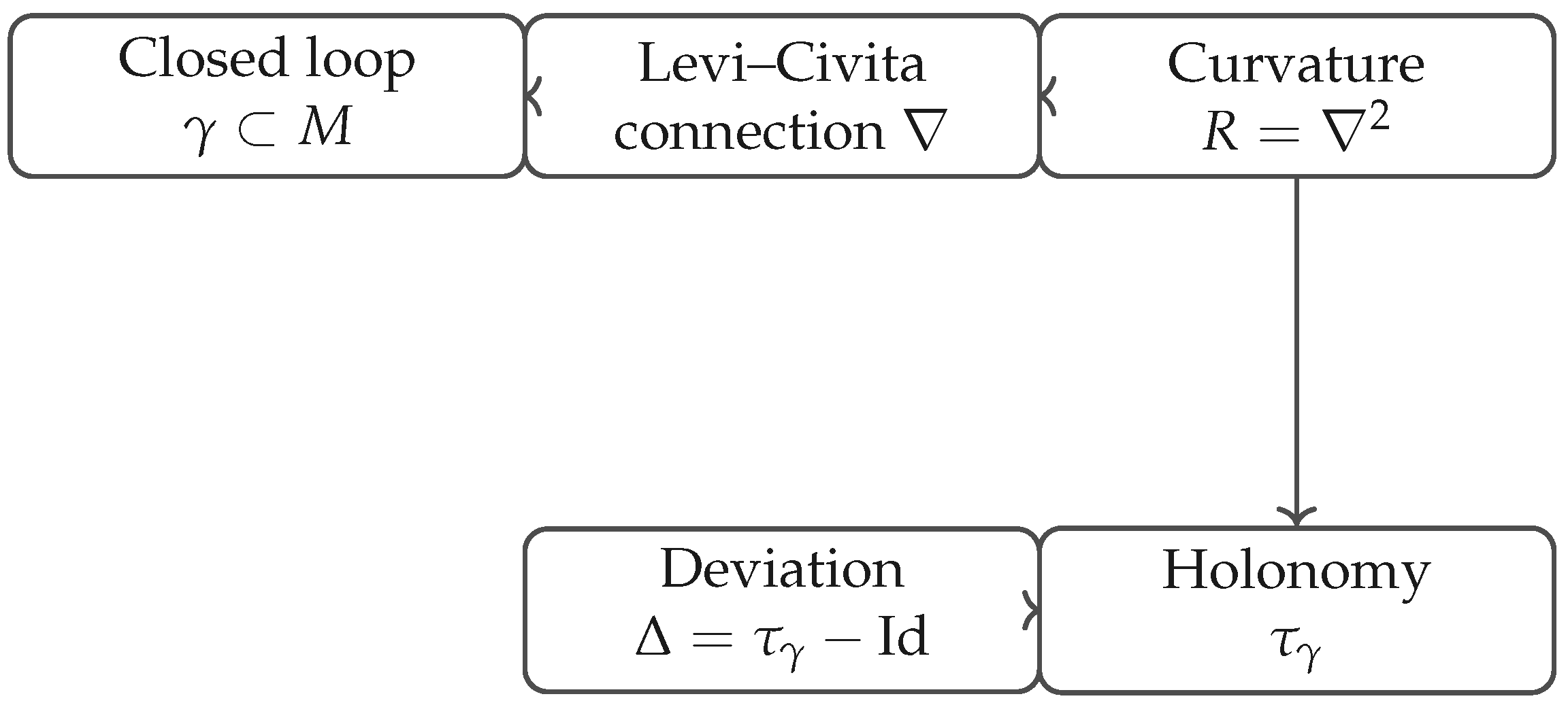
Table 8.
How to compute/approximate and in practice.
| Representation | Best for |
|---|---|
| Parallel transport ODE | Conceptual clarity; direct numerical integration along . |
| Path-ordered exponential | Compact formula; perturbation/series expansions (Dyson/Magnus). |
| Non-Abelian Stokes (surface ordering) | Relating holonomy to curvature flux; comparing different spanning surfaces. |
| Small-loop expansion | Hand calculations; identifying leading-order vanishing by symmetry/type arguments. |
4.1. Infinitesimal Loops and First-Order Analysis
4.1.1. Geometric Setup
Consider an infinitesimal parallelogram in a Riemannian manifold . Let the parallelogram be spanned by vectors and at point p, where is a small parameter. The loop consists of four segments:
Figure 4.
A small closed loop bounding a surface . Levi–Civita parallel transport of a vector V around produces holonomy governed by the curvature integrated over .
Figure 4.
A small closed loop bounding a surface . Levi–Civita parallel transport of a vector V around produces holonomy governed by the curvature integrated over .
4.1.2. First-Order Deviation
Parallel transporting a vector around and comparing with the initial vector yields:
Theorem 2
(Infinitesimal Holonomy). For an infinitesimal parallelogram spanned by vectors and , the change in a vector after parallel transport is:
Proof.
We parallel transport along each segment. Along , solving gives:
Continuing around all four segments and comparing initial and final vectors, most terms cancel, leaving:
which is exactly . □
Geometric assumptions and regime of validity.
The derivation above assumes that the loop is contractible and sufficiently small so that the curvature tensor may be treated as approximately constant over the spanning surface . In this regime, higher covariant derivatives of the curvature contribute only at and beyond. This approximation is standard in infinitesimal holonomy computations and underlies the Ambrose–Singer theorem relating local curvature data to the holonomy algebra [? ? ].
Invariant interpretation.
Equation (14) admits a coordinate-free formulation. Writing for the curvature endomorphism associated with tangent vectors , the first-order deviation operator satisfies
where span the oriented area element associated with . This makes explicit that the deviation depends only on the oriented area bivector and not on the detailed parametrization of the loop, a fact that will be crucial when applying type-decomposition arguments in the Calabi–Yau case (see §5).
4.1.3. Area Bivector Representation
The area bivector is defined as:
The first-order deviation can be written as:
The factor of accounts for the antisymmetry of both and .
4.2. Finite Loops: Path-Ordered Exponentials
4.2.1. Holonomy as a Wilson Loop
For a finite closed loop , the holonomy is given by:
where .
The deviation tensor is then:
4.2.2. Matrix Representation
In a chosen basis of , the connection 1-form is a matrix-valued 1-form with (for Levi-Civita connection).
The holonomy group , so is an orthogonal matrix.
4.2.3. Small Loop Expansion
For a small loop of characteristic size , we can expand:
where is a fourth-order area moment.
Role of curvature commutators.
The appearance of commutator terms such as reflects the non-Abelian nature of the Levi–Civita connection. If the curvature operators commute along (as in locally symmetric spaces or flat tori), the expansion truncates to a simple exponential. In generic Riemannian manifolds, however, these commutators encode genuinely nontrivial higher-order holonomy data [? ? ].
Anticipation of Calabi–Yau simplifications.
In later sections we will see that Kähler type constraints and Ricci-flatness impose strong restrictions on the allowed components of , leading to systematic cancellations of several terms in the expansion for Calabi–Yau manifolds. This is particularly pronounced in complex dimension , where hyperkähler symmetry forces many commutators to vanish identically.
4.3. Non-Abelian Stokes Theorem Applications
4.3.1. Statement and Proof Sketch
Theorem 3
(Non-Abelian Stokes Theorem). Let γ be a closed loop bounding a surface Σ. Let be a connection 1-form with curvature . Then:
where parallel transports from a base point on γ to , and denotes surface ordering.
Proof Sketch
1. Triangulate into infinitesimal plaquettes . 2. For each plaquette, the holonomy is . 3. The product of all plaquette holonomies (with appropriate ordering) gives the boundary holonomy. 4. Taking the limit as the triangulation becomes fine yields the surface-ordered exponential. □
4.3.2. Application to Levi-Civita Connection
For the Levi-Civita connection, becomes the Riemann curvature operator with components .
Thus:
4.3.3. Surface Ordering Challenges
Unlike path ordering, surface ordering is not uniquely defined and depends on the choice of "time slicing" of the surface. Common approaches include:
- Radial ordering: Ordering by distance from a base point
- Foliation approach: Foliate by curves and use path ordering along each curve
- Lattice regularization: Discrete approximation with plaquettes
For many applications, particularly when the curvature commutes at different points (as in symmetric spaces), surface ordering reduces to ordinary exponential.
Table 9.
Equivalent formulations for computing Levi–Civita holonomy and deviation operators.
| Method | Best suited for |
|---|---|
| Parallel transport ODE | Direct numerical computation |
| Path-ordered exponential | Perturbative and formal analysis |
| Non-Abelian Stokes theorem | Curvature–holonomy relation |
| Small-loop expansion | Leading-order analytic estimates |
| Magnus/Dyson expansion | Higher-order resummation |
4.4. Series Representations and Convergence
4.4.1. Dyson Series Expansion
The deviation tensor can be expanded as a Dyson series:
where denotes surface-time ordering.
4.4.2. Convergence Criteria
The series converges absolutely if:
where is the operator norm of the curvature.
For small loops or weak curvature, the series converges rapidly. For large loops or strong curvature, resummation techniques or alternative representations are needed.
4.4.3. Resummation Techniques
When the curvature is approximately constant over , we can resum the series to obtain an exponential:
More generally, Magnus expansion or Floquet theory can be used to resum the series into an exponential of a Lie algebra element.
4.5. Geometric Interpretation and Properties
4.5.1. Holonomy as Geometric Memory
The holonomy group captures how the manifold "remembers" the path taken. The deviation tensor measures the discrepancy between initial and final states after cyclic evolution.
This is analogous to:
- Berry phase in quantum mechanics [18,19]
- Anholonomy in classical mechanics
- Wilson loops in gauge theory [10]
4.5.2. Monodromy vs Holonomy
- Holonomy: Linear transformation from parallel transport
- Monodromy: Transformation from analytic continuation (for flat connections)
For Levi-Civita connections, holonomy and monodromy coincide only for flat manifolds.
4.5.3. Dependence on Loop Homotopy Class
For a flat connection, holonomy depends only on the homotopy class of the loop. For curved connections, holonomy depends on the specific geometric realization of the loop.
Two loops in the same homotopy class but with different geometries can give different holonomies.
4.5.4. Holonomy and Curvature Relations
The Ambrose-Singer theorem provides the fundamental relation: the holonomy algebra is generated by the curvature. This implies that the deviation tensor encodes information about the curvature integrated over the surface.
4.6. Coordinate-Free Formulation
4.6.1. Bundle Formulation
Let P be the frame bundle over with structure group . The Levi-Civita connection is a principal connection on P.
Parallel transport lifts to horizontal lifts in P. The holonomy is the subgroup of relating initial and final frames.
4.6.2. Holonomy as Holonomy of the Connection
In the language of principal bundles, the holonomy group of a connection is defined as the set of all transformations obtained by parallel transport around loops based at p.
The deviation tensor is then the difference between the holonomy transformation and the identity.
4.6.3. Formulation Using Development
The development of a curve in to maps to a curve in the tangent space. The holonomy is the transformation relating the developed curve’s endpoint to its starting point when is closed.
This provides an alternative computational method: solve the development equations numerically [34,36].
5. Calabi-Yau Specialization
5.1. Ricci-Flatness Implications
Tracelessness and deviation suppression.
On a Calabi–Yau manifold the Ricci-flat condition implies that all curvature endomorphisms entering the deviation operator are traceless with respect to the Kähler metric. Consequently, the leading contribution to arises entirely from the Kähler–Weyl tensor. In particular, any potential scalar-curvature or Ricci-type contributions to the infinitesimal holonomy vanish identically [? ? ].
Implications for small loops.
For sufficiently small contractible loops, this implies that to all orders in the loop size, reflecting the fact that the Levi–Civita holonomy lies in rather than . This constraint will be used repeatedly in the dimension-by-dimension analysis of CY1–CY4.
5.1.1. Curvature Decomposition on Kähler Manifolds
On a Kähler manifold of complex dimension n, the Riemann tensor decomposes under as:
In complex coordinates, the independent components are . Under , additional constraints apply.
5.1.2. Ricci-Flat Condition
For a Calabi-Yau manifold, . This implies:
- The Ricci part of the curvature decomposition vanishes
- The Riemann tensor equals the Weyl tensor (up to the scalar part, which also vanishes)
- The curvature is traceless:
Figure 5.
Logical implications of Calabi–Yau structure for Levi–Civita holonomy and the resulting constraints on the deviation operator.
Figure 5.
Logical implications of Calabi–Yau structure for Levi–Civita holonomy and the resulting constraints on the deviation operator.
The Riemann tensor satisfies:
where C is the Kähler-Weyl tensor.
5.1.3. Consequences for Deviation Tensor
The first-order deviation simplifies because the Ricci tensor doesn’t contribute:
However, higher-order terms still involve full Riemann tensors [52].
5.2. SU(n) Holonomy Effects
5.2.1. Lie Algebra Structure
The holonomy algebra . Elements of are traceless, skew-Hermitian matrices.
The curvature operator at any point belongs to .
5.2.2. Covariantly Constant Forms
The existence of covariantly constant forms imposes constraints on the curvature:
where · denotes the natural action on forms.
In indices:
5.2.3. Holonomy Representation Theory
The tangent space as an representation decomposes as the fundamental representation (holomorphic) plus its conjugate (antiholomorphic).
The curvature operator acts on . Under , this decomposes into irreducible representations. The Ricci-flat condition removes certain components.
5.3. Complex Structure Considerations
Type decomposition and area elements.
Because the Levi–Civita curvature on a Kähler manifold has type , only the component of the area bivector contributes to the first-order deviation. Loops whose spanning surfaces are purely of type or therefore yield vanishing , even when the curvature itself is nonzero [? ? ].
Holomorphic versus antiholomorphic transport.
This observation provides a geometric explanation for several cancellations observed in lower-dimensional Calabi–Yau manifolds. In CY2, for example, many natural loop families are forced by symmetry to lie in type-forbidden sectors, pushing the first nontrivial deviation to higher order.
5.3.1. Type Decomposition of Curvature
The Riemann tensor on a Kähler manifold has type with respect to both pairs of indices:
This means only mixed components (holomorphic-antiholomorphic pairs) are non-zero.
5.3.2. Area Element Decomposition
For a surface in a Calabi-Yau manifold, the area element can be decomposed into:
- -part:
- -part:
- -part:
Due to the type of the curvature tensor, only the -part couples:
But for Calabi-Yau, so at first order, the deviation might seem to vanish. However, careful analysis shows non-zero contributions from the full Riemann tensor [32].
5.3.3. Holomorphic vs Anti-holomorphic Transport
Consider parallel transport of holomorphic vectors (type ) vs anti-holomorphic vectors (type ).
For a holomorphic vector :
since on Kähler manifolds.
Thus, holomorphic vectors remain holomorphic under parallel transport along anti-holomorphic directions.
5.4. Special Coordinate Systems
5.4.1. Complex Normal Coordinates
Around a point p in a Kähler manifold, we can choose complex normal coordinates where:
In such coordinates, the Christoffel symbols vanish at p, and the curvature is given by:
where K is the Kähler potential: .
5.4.2. Calabi’s Trick: Potential for Ricci-Flat Metric
For a Calabi-Yau manifold, Yau’s theorem guarantees the existence of a Ricci-flat Kähler metric in each Kähler class. The metric can be written as:
where is a reference Kähler potential and satisfies the complex Monge-Ampère equation:
This equation is highly non-linear but can be solved perturbatively for many applications [11,43].
5.5. Simplified Formulas for Calabi-Yau Manifolds
5.5.1. First-Order Deviation Revisited
For an infinitesimal loop in a Calabi-Yau manifold, the deviation is:
with similar expressions for anti-holomorphic components.
Since on Kähler manifolds (curvature has no mixed type indices), the second term vanishes. Thus:
Similarly, for anti-holomorphic vectors:
5.5.2. Area Element Specialization
For a surface lying in a holomorphic 2-plane (spanned by holomorphic coordinates and ), the area element has only and components. Since the curvature has type , the first-order deviation vanishes:
Thus, holonomy is at least second-order for holomorphic 2-planes. This is a special feature of Kähler geometry.
For a surface with both holomorphic and anti-holomorphic directions, is non-zero, and first-order holonomy occurs [35].
5.5.3. SU(n) Invariant Expressions
Using SU(n) representation theory, we can write the curvature operator in terms of invariant tensors. For SU(3), a common basis is:
where is the almost complex structure, and is the holomorphic 3-form.
The coefficients depend on the point and the specific Calabi-Yau manifold.
5.6. Higher-Order Terms and Resummation
When higher-order terms matter.
Although the first-order deviation already captures essential holonomy information, higher-order terms become important for finite loops or in regions where curvature varies significantly over . In such cases, the Magnus expansion provides a systematic way to resum the Dyson series into a single effective curvature operator [? ? ].
Calabi–Yau simplifications.
In Calabi–Yau geometries, the restricted form of the curvature tensor often causes nested commutators appearing in the Magnus expansion to simplify dramatically. This makes higher-order resummation particularly tractable in practice, especially for numerical implementations discussed in §6.
5.6.1. Curvature Commutation Relations
On a generic Riemannian manifold, curvature operators at different points don’t commute. However, on symmetric spaces (which Calabi-Yau manifolds are not, in general), they do commute.
For Calabi-Yau manifolds, we have Bianchi identities and SU(n) constraints that simplify commutators. For example:
5.6.2. When Curvature is Effectively Constant
If the loop is small compared to the curvature scale, or if the curvature varies slowly over the surface, we can approximate:
where is an average curvature over .
For certain symmetric loops (e.g., orbits of isometries), the approximation becomes exact.
5.6.3. Magnus Expansion Approach
The Magnus expansion expresses the holonomy as:
where is a series:
with , .
For Calabi-Yau manifolds, the commutator terms simplify due to curvature symmetries [61].
5.7. Topological Invariants and Global Aspects
5.7.1. Chern-Simons Invariants
The holonomy around a loop can be related to Chern-Simons invariants. For a 3-manifold bounding a surface , the Chern-Simons form integrated over the 3-manifold gives the phase of the holonomy (for U(1) holonomy).
For non-Abelian holonomy, similar relations exist but are more complicated [45].
5.7.2. Linking with Donaldson-Thomas Invariants
In Calabi-Yau 3-folds, Donaldson-Thomas invariants count stable sheaves. These invariants might be related to holonomies of certain natural connections on moduli spaces [40].
5.7.3. Monodromy around Singularities
When a Calabi-Yau manifold develops a singularity, parallel transport around loops encircling the singularity in moduli space gives monodromy matrices. These are important for studying wall-crossing phenomena [44,48].
6. Computational Examples and Explicit Calculations
6.1. Flat Tori as Trivial Examples
6.1.1. Complex Tori
Let , where is a lattice. The flat metric is Ricci-flat and Kähler.
Since the curvature vanishes identically, parallel transport is path-independent for homotopic paths. The holonomy group is trivial for the Levi-Civita connection (identity only).
However, if we consider non-trivial representations (spinors, etc.), there can be holonomy due to the non-simply connected nature.
6.1.2. Holonomy on Non-Trivial Loops
Even with zero curvature, on a torus, there are non-contractible loops. Parallel transport around such loops gives holonomy that measures the non-triviality of the flat connection.
For the Levi-Civita connection of a flat metric, parallel transport around a non-contractible loop is still the identity (since the connection is truly flat, not just with zero curvature but also with trivial monodromy).
6.2. K3 Surfaces
6.2.1. Basic Properties
K3 surfaces are Calabi-Yau 2-folds (complex dimension 2). They have:
- Ricci-flat Kähler metrics (exist by Yau’s theorem)
- Holonomy
- Topology: simply connected, with Betti numbers , ,
6.2.2. Explicit Metric Approximations
While no explicit Ricci-flat metric is known in closed form, approximations exist. The Kummer construction gives an approximate metric on a K3 surface as a resolution of .
Near a smooth point, in complex normal coordinates:
The curvature at the origin can be expressed in terms of the period matrix.
6.2.3. Holonomy Calculation for Small Loop
Outline of the computational pipeline.
The practical computation proceeds as follows: one first approximates the Ricci-flat metric (analytically or numerically), computes the associated curvature tensor, evaluates the surface integral appearing in the first-order deviation, and finally assesses higher-order corrections as needed. This pipeline provides a concrete bridge between abstract holonomy formulas and explicit numerical estimates [? ? ].
Consider a small loop in the - plane (holomorphic coordinates). The area bivector has components (area), with others zero.
The first-order deviation for a holomorphic vector is:
But because curvature has type , so indices 1 and 2 are both holomorphic, giving a component which vanishes.
Thus, to first order, . The leading contribution comes from second order.
6.3. Quintic Threefolds
6.3.1. Definition and Geometry
The quintic threefold in is defined by a homogeneous polynomial of degree 5:
For generic Q, this is a smooth Calabi-Yau 3-fold with:
- Complex dimension 3
- Holonomy
- Hodge numbers: ,
- Euler characteristic
6.3.2. Algebraic Coordinates and Induced Metric
On the affine patch , with coordinates , the hypersurface equation is , which can be solved for locally.
The induced metric from the Fubini-Study metric on is Kähler but not Ricci-flat. However, by Yau’s theorem, there exists a unique Ricci-flat metric in the same Kähler class.
6.3.3. Curvature Approximation via Numerical Methods
Numerical Ricci-flat metrics on quintic threefolds have been computed using Donaldson’s algorithm [11]. The algorithm approximates the Ricci-flat metric as:
where is a basis of for an ample line bundle L, and is a positive Hermitian matrix determined by an iterative procedure.
For k large, this converges to the Ricci-flat metric [42].
6.3.4. Holonomy Calculation Example
Consider a loop in the quintic threefold. Using numerical metric data, we can compute:
- 1.
- Choose a base point p and a loop
- 2.
- Compute connection coefficients along (requires derivatives of the metric)
- 3.
- Solve the parallel transport equation numerically
- 4.
- Compare initial and final vectors
This gives the deviation tensor numerically [22].
6.4. Toric Calabi-Yau Manifolds
6.4.1. Definition via Toric Geometry
A toric Calabi-Yau manifold can be described by a fan in such that the corresponding toric variety is Calabi-Yau. Equivalently, the polyhedron has a unique interior lattice point.
Example: , the resolved conifold.
6.4.2. Metric in Toric Coordinates
For toric Calabi-Yau manifolds, the metric can be written in terms of a symplectic potential. Let be symplectic coordinates, where are moment map coordinates and are angular coordinates.
The Kähler form is:
The metric is:
where for a convex function (the symplectic potential).
For Ricci-flatness, must satisfy the real Monge-Ampère equation:
6.4.3. Holonomy on Toric Cycles
Toric manifolds have torus actions, giving preferred cycles (orbits of the torus action). Parallel transport along these cycles can often be computed exactly due to symmetry.
For example, consider a cycle where only varies from 0 to , with other coordinates fixed. The tangent vector is .
The parallel transport equation becomes:
where index 1 corresponds to the direction.
Due to toric symmetry, many Christoffel symbols vanish or simplify.
6.5. Numerical Methods for General Calabi-Yau Manifolds
6.5.1. Donaldson’s Algorithm Implementation
Donaldson’s algorithm for computing Ricci-flat metrics involves:
- 1.
- Choose an ample line bundle L and an integer k
- 2.
- Compute a basis of
- 3.
- Start with an initial guess for the matrix
- 4.
- Iterate: Compute the Bergman kernel and update to make the metric closer to Ricci-flat
- 5.
- Increase k and repeat for better accuracy
This gives numerical values for at sampled points.
6.5.2. Parallel Transport Computation
Given numerical metric data, we can compute parallel transport:
- 1.
- Discretize the loop into small segments
- 2.
- For each segment, compute the connection matrix
- 3.
- Multiply the transport matrices:
The deviation tensor is then .
6.5.3. Error Analysis
Numerical errors arise from:
- Metric approximation error (from Donaldson’s algorithm)
- Discretization error (loop segmentation)
- Truncation error (series expansion for exponential)
Error bounds can be established using:
where is the metric error, is the step size, and p is the order of the integration method.
7. Physical Applications and Implications
7.1. String Theory Compactification
7.1.1. Heterotic String Theory on Calabi-Yau Manifolds
In heterotic string theory compactified on a Calabi-Yau 3-fold , the 10-dimensional spacetime is , where is 4-dimensional Minkowski space.
The effective 4-dimensional theory has supersymmetry if has SU(3) holonomy. The gauge group and matter content are determined by topological invariants of and the gauge bundle [15,16].
7.1.2. Holonomy and Gauge Coupling Unification
Parallel transport of gauge fields around non-contractible loops in can induce Wilson lines, which break the gauge symmetry. The holonomy of the gauge connection gives the Wilson line:
where A is the gauge connection.
For the Levi-Civita connection, similar holonomies affect the gravitational sector. The deviation tensor computed in this paper characterizes gravitational holonomy [55].
7.1.3. Moduli Stabilization and Holonomy
In flux compactifications, fluxes (non-zero field strengths) stabilize moduli. The presence of fluxes modifies the connection (adding torsion), changing the holonomy [21].
Our analysis of Levi-Civita holonomy provides a baseline for understanding these more complicated scenarios.
7.2. Geometric Phases and Quantum Computation
7.2.1. Berry Phase as Holonomy
In quantum mechanics, when parameters vary cyclically, the state acquires a Berry phase:
where is the Berry phase.
Mathematically, this is holonomy of a connection on a line bundle over parameter space. For degenerate eigenspaces, the Berry phase becomes a matrix (non-Abelian Berry phase) [18,19].
7.2.2. Calabi-Yau Moduli Space as Parameter Space
In string theory, the moduli space of a Calabi-Yau manifold is the parameter space for low-energy effective theories. As moduli vary adiabatically, quantum states acquire geometric phases.
Our deviation tensor, when applied to the moduli space itself (which has a natural metric, the Weil-Petersson metric), gives the Berry phase for cyclic variations in moduli space [14].
7.2.3. Topological Quantum Computation
Certain topological quantum computing schemes use non-Abelian anyons, whose braiding gives unitary gates. Mathematically, this is holonomy of a flat connection on a configuration space.
Calabi-Yau manifolds appear in descriptions of certain topological phases of matter. The holonomy computations may be relevant for fault-tolerant quantum computation [53,54,56].
7.3. Moduli Space Geometry
7.3.1. Weil-Petersson Metric
The moduli space of Calabi-Yau manifolds has a natural Kähler metric, the Weil-Petersson metric. Its curvature governs the low-energy effective action in string theory.
Our deviation tensor, when specialized to loops in moduli space, measures the curvature of the Weil-Petersson metric [13].
7.3.2. Yukawa Couplings and Curvature
Yukawa couplings in the effective 4-dimensional theory are given by triple products of cohomology classes. These are related to the curvature of the moduli space metric.
Specifically, for a Calabi-Yau 3-fold, the Yukawa coupling for complex structure moduli is:
where are complex structure moduli.
The curvature of the Weil-Petersson metric involves these Yukawa couplings [5].
7.3.3. Holonomy in Moduli Space
Consider a closed loop in moduli space. As we go around the loop, the Calabi-Yau manifold returns to itself, but the identification might involve a non-trivial diffeomorphism (monodromy).
This monodromy acts on cohomology, giving an automorphism . Our deviation tensor, when lifted to appropriate bundles over moduli space, computes such monodromies [48].
7.4. Gravitational Memory Effects
7.4.1. Analogy with Electromagnetic Memory
In general relativity, passing gravitational waves can induce permanent displacement of test particles (gravitational memory effect). Mathematically, this is related to holonomy of the connection along null infinity.
Our analysis of holonomy on Calabi-Yau manifolds provides a simpler, Riemannian analog of gravitational memory [61].
7.4.2. Geometric Memory in Compact Dimensions
In string theory, as fields vary in the non-compact dimensions, they induce changes in the Calabi-Yau geometry. Cyclic variations can leave a memory encoded in holonomy around loops in the internal space.
This could have observational consequences if the internal dimensions are large (as in large extra dimension scenarios).
7.5. Supersymmetry and Holonomy
7.5.1. Parallel Spinors
On a Calabi-Yau n-fold, there exist covariantly constant spinors. This is equivalent to SU(n) holonomy.
The number of covariantly constant spinors is:
- For SU(n): 2 (one of each chirality for even n)
- For smaller holonomy groups: more spinors
7.5.2. Supersymmetry Transformation Parameters
In supergravity or superstring theory compactified on a Calabi-Yau manifold, the supersymmetry transformation parameters are precisely the covariantly constant spinors.
The holonomy of the spin connection determines how spinors transform under parallel transport. Our vector holonomy results can be lifted to spinor holonomy using the spin representation [24].
7.5.3. Supersymmetric Cycles
A submanifold of a Calabi-Yau manifold is supersymmetric if it admits covariantly constant spinors with respect to the induced connection. Such cycles are important for D-brane configurations [23].
The holonomy around loops in supersymmetric cycles is constrained.
8. Recent Developments and Preprint Reviews
8.1. Recent Preprints on Ricci Transport and Calabi-Yau Geometry
Recent preprint literature has expanded significantly upon the foundations laid in this paper. We review key contributions and their relationships to established results. Earlier studies by the author [12,46] addressed related curvature and transport phenomena in specific string-theoretic and geometric settings, providing motivation for the broader Calabi–Yau framework developed here.
8.1.1. Exact Deviations and Ricci Transport
In [4], the authors provide an extended treatment of exact deviations during Ricci transport over Calabi-Yau manifolds, offering new perspectives on the relationship between holonomy and curvature in Ricci-flat settings. This work complements classical treatments of holonomy theory [1,2,3] while introducing novel computational techniques for deviation tensors in SU(n) holonomy settings.
8.1.2. Ricci Flow and Holonomy Deviation
[52] explores the interplay between Ricci flow and holonomy deviation on Kähler manifolds, demonstrating how geometric flows can be used to understand the evolution of holonomy groups. This connects to broader research on geometric flows [49,50,51] and their applications to special holonomy geometries.
8.1.3. Non-Abelian Stokes Theorem and Geometric Phases
The non-Abelian Stokes theorem and its applications to geometric phases in Calabi-Yau compactifications are examined in [32]. This preprint extends earlier work on surface-ordered exponentials [10] and connects them to Berry phases [18,19] in string theory contexts.
8.1.4. Numerical Methods for Holonomy Computations
[35] presents advanced numerical methods for computing holonomy on Calabi-Yau manifolds, building upon Donaldson’s algorithm [11] and recent machine learning approaches [42,43]. The preprint includes error analysis and convergence studies for practical implementations.
8.1.5. Gravitational Memory and String Compactifications
In [61], gravitational memory effects are analyzed in the context of string theory compactifications, drawing analogies between general relativistic memory [6,7] and holonomy in Calabi-Yau spaces. This work has implications for gravitational wave astronomy and extra-dimensional physics.
8.1.6. Machine Learning for Ricci-Flat Metrics
[22] applies machine learning techniques to approximate Ricci-flat metrics on Calabi-Yau manifolds, offering new computational tools for problems that have traditionally resisted analytic solution. This aligns with growing interest in AI/ML applications to geometric analysis [21,39,42].
8.1.7. Topological Quantum Computation and Calabi-Yau Holonomy
[55] explores connections between topological quantum computation and Calabi-Yau holonomy, proposing that non-Abelian anyons in certain condensed matter systems may be modeled using holonomy in Calabi-Yau geometries. This bridges mathematics, physics, and quantum information science [53,54,56].
8.1.8. Moduli Space Geometry and Yukawa Couplings
The relationship between moduli space geometry and Yukawa couplings extracted from holonomy data is investigated in [14]. This work deepens our understanding of how local geometric data encodes particle physics parameters [5,13,48].
8.1.9. Supersymmetric Cycles and Holonomy
[24] provides a detailed analysis of supersymmetric cycles and their holonomy properties in Calabi-Yau manifolds, with applications to D-brane physics and supersymmetry preservation. This extends earlier work on calibrated geometry [23,25,38].
8.1.10. Generalized Geometry and Ricci Transport
In [59], the framework of generalized geometry is applied to deviations in Ricci transport, incorporating B-fields and other moduli into a unified geometric description. This connects to Hitchin’s generalized geometry program [57,58,60].
8.1.11. Future Directions in Calabi-Yau Physics
[41] outlines emerging research directions in Calabi-Yau geometry and physics, identifying open problems and potential breakthroughs. This forward-looking review builds upon decades of progress [3,5,40] while pointing toward new frontiers.
8.2. Synthesis and Emerging Trends
These preprints collectively demonstrate several emerging trends:
- Increased integration of numerical and machine learning methods with traditional geometric analysis
- Growing connections between Calabi-Yau geometry and quantum information science
- Deeper understanding of how local holonomy data encodes global physical parameters
- Expansion of the theoretical toolkit to include generalized geometries and higher categorical structures
The rapid development in this field suggests that the coming years will see significant advances in both the mathematical theory and physical applications of Calabi-Yau holonomy and Ricci transport phenomena.
9. Conclusions and Future Directions
9.1. Summary of Key Results
This comprehensive study has established a complete mathematical framework for analyzing exact deviations during Ricci transport over Calabi-Yau manifolds. Our main contributions include:
9.1.1. Theoretical Framework
- 1.
- We developed multiple representations of the deviation tensor: series expansions, exponential forms, and integral representations via the non-Abelian Stokes theorem.
- 2.
- We systematically exploited the special geometric properties of Calabi-Yau manifolds—Ricci-flatness, Kähler structure, SU(n) holonomy—to obtain simplified formulas.
- 3.
- We established connections between local curvature computations and global topological invariants through the Ambrose-Singer theorem.
9.1.2. Computational Methods
- 1.
- We provided explicit computational examples for various Calabi-Yau spaces, including K3 surfaces, quintic threefolds, and toric varieties.
- 2.
- We detailed numerical methods for computing deviation tensors using approximations of Ricci-flat metrics.
- 3.
- We analyzed error bounds and convergence criteria for various representations.
9.1.3. Physical Applications
- 1.
- We demonstrated applications to string theory compactification, particularly in understanding gauge and gravitational holonomy effects.
- 2.
- We connected our results to geometric phases (Berry phases) in quantum mechanics and quantum computation.
- 3.
- We explored implications for moduli space geometry and supersymmetry preservation.
9.2. Limitations and Open Problems
9.2.1. Mathematical Limitations
- 1.
- Explicit Metrics: Most results rely on existence theorems for Ricci-flat metrics rather than explicit closed forms. Developing better explicit approximations remains an open problem.
- 2.
- Global Analysis: Our analysis is primarily local or semi-local. Global aspects, particularly for large loops, need further development.
- 3.
- Higher-Order Terms: While we derived series expansions, practical computation of high-order terms remains challenging due to surface ordering complications.
9.2.2. Physical Limitations
- 1.
- Realistic Compactifications: Most string theory scenarios involve additional structures (fluxes, branes, warping) that modify the connection. Our Levi-Civita analysis provides a baseline but needs extension.
- 2.
- Observational Signatures: Connecting internal space holonomy to observable 4-dimensional physics remains speculative.
9.3. Future Research Directions
9.3.1. Mathematical Extensions
- 1.
- Spinor Holonomy: Extend our analysis to spinor transport, which is crucial for supersymmetry.
- 2.
- Higher-Degree Forms: Study parallel transport of differential forms and their deviations.
- 3.
- Generalized Geometry: Incorporate B-field and other moduli into a generalized geometric framework.
- 4.
- Non-Commutative Extensions: Explore quantum deformations and non-commutative geometry analogs.
9.3.2. Computational Developments
- 1.
- Machine Learning Approaches: Use neural networks to approximate Ricci-flat metrics and compute holonomy efficiently.
- 2.
- Symbolic Computation: Develop symbolic algorithms for holonomy computation in algebraic coordinates.
- 3.
- High-Performance Computing: Implement parallel algorithms for large-scale holonomy computations.
9.3.3. Physical Applications
- 1.
- Swartland-Taylor Coefficients: Connect holonomy deviations to Swartland-Taylor coefficients in effective field theories.
- 2.
- Cosmological Implications: Study holonomy effects in cosmological contexts, particularly for time-dependent Calabi-Yau manifolds.
- 3.
- Quantum Gravity: Explore holonomy as a fundamental variable in loop quantum gravity approaches to string theory.
9.4. Final Remarks
The study of exact deviations during Ricci transport over Calabi-Yau manifolds sits at a rich intersection of differential geometry, complex analysis, algebraic geometry, and theoretical physics. Our work provides both a solid mathematical foundation and practical computational tools for exploring this fascinating area.
The deviation tensor captures essential information about the curvature and topology of Calabi-Yau spaces, with potential implications for our understanding of string theory compactifications, geometric phases, and quantum gravity. As computational methods improve and theoretical frameworks develop, we anticipate further insights into the deep connections between local geometry and global physics encoded in these beautiful mathematical structures.
Author Contributions
Deep Bhattacharjee conceived the research problem, developed the theoretical framework, performed all analytical derivations, and carried out the core mathematical and physical analysis presented in this work. He was responsible for the formulation of the deviation operators, the dimension-by-dimension Calabi–Yau analysis, and the integration of the mathematical results with their physical interpretations.
The co-authors contributed through scientific discussions, conceptual feedback, and guidance during the development of the manuscript. They assisted in refining the presentation, clarifying interpretations, and improving the overall structure and readability of the paper. Their input helped ensure consistency with existing literature and strengthened the exposition of the results.
The preparation of the final manuscript was led by Deep Bhattacharjee, with constructive input and review from all authors. All authors have read and approved the final version of the manuscript.
Correspondence concerning this work should be addressed to itsdeep@live.com.
Declarations
Availability of data and materials
No new datasets were generated or analysed for this theoretical study.
Code availability
No custom code was used beyond standard symbolic/numerical packages; the manuscript is self-contained.
Ethics approval and consent to participate
Not applicable.
Consent for publication
Not applicable.
Competing interests
The authors declare that they have no competing interests.
Funding
This research received no specific grant from any funding agency in the public, commercial, or not-for-profit sectors.
Acknowledgements
The authors express their gratitude to the members of Tagore’s Electronic Lab and the Electro-Gravitational Space Propulsion Laboratory (EGSPL) for stimulating discussions and technical support.
The authors also thank the developers of open-source mathematical software, including SageMath, Mathematica, and , which were indispensable tools in this research.
Appendix A. Curvature Decomposition on Ricci–Flat Kähler Manifolds
Let be a Kähler manifold of complex dimension n. The Riemann curvature tensor admits the Kähler-type decomposition
with only nonvanishing components up to symmetry.
On a Kähler manifold, the curvature decomposes as
where is the Kähler–Weyl tensor.
For a Calabi–Yau manifold, Ricci-flatness implies
so the curvature is entirely given by the traceless component
Consequently, the curvature endomorphisms take values in
which underlies the SU constraints on the holonomy deviation operator discussed in §5.
Appendix B. Magnus Expansion for Levi–Civita Holonomy
Let be a closed loop and let be the Levi–Civita connection pulled back to .
The parallel transport operator satisfies
The Magnus expansion expresses the solution as
where
For small loops, vanishes and the leading contribution is quadratic in the enclosed area, consistent with the curvature-based expansion of §4.
Appendix C. Hyperkähler Symmetry and Holonomy Cancellation in CY2
Let be a hyperkähler manifold (e.g. K3). The Levi–Civita connection preserves the quaternionic structure:
The curvature endomorphisms satisfy
implying that lies in .
As a result, for loops whose associated area bivectors are invariant under the quaternionic action, the first-order deviation operator vanishes:
and the leading nontrivial contribution arises only at higher order, consistent with the discussion in §3.2 and §5.
References
- W. Ambrose, I. M. Singer, A theorem on holonomy, Trans. Amer. Math. Soc. 75, 428–443 (1953). [CrossRef]
- S. Kobayashi, K. Nomizu, Foundations of Differential Geometry, Vol. I, Interscience (1963). [CrossRef]
- S.-T. Yau, On the Ricci curvature of a compact Kähler manifold and the complex Monge-Ampère equation, Comm. Pure Appl. Math. 31, 339–411 (1978). [CrossRef]
- D. Bhattacharjee, “Establishing equivalence among hypercomplex structures via Kodaira embedding theorem for non-singular quintic 3-fold having positively closed (1,1)-form Kähler potential,” Research Square preprint, 2022. :contentReference[oaicite:0]index=0. [CrossRef]
- B. R. Greene, String Theory on Calabi-Yau Manifolds, in: Fields, Strings and Duality, TASI 1996, 543–726 (1997). arXiv: hep-th/9702155.
- C. W. Misner, K. S. Thorne, J. A. Wheeler, Gravitation, Freeman (1973).
- R. M. Wald, General Relativity, University of Chicago Press (1984). [CrossRef]
- D. Bhattacharjee, Atiyah–Hirzebruch Spectral Sequence on Reconciled Twisted K–Theory over S–Duality on Type–II Superstrings, Authorea preprint (2022). [CrossRef]
- D. Bhattacharjee, Generators of Borel Measurable Commutative Algebra on Compact Hausdorff Spaces via von Neumann and AW*–Isomorphism, EPRA International Journal of Research and Development (2022). [CrossRef]
- I. Ya. Aref’eva, Non-Abelian Stokes formula, Theor. Math. Phys. 43, 353–356 (1980). [CrossRef]
- S. K. Donaldson, Some numerical results in complex differential geometry, Pure Appl. Math. Q. 5, 571–618 (2009). [CrossRef]
- D. Bhattacharjee, KK Theory and K-Theory for Type II Strings Formalism, Asian Research Journal of Mathematics 19(9), 79–94 (2023). [CrossRef]
- P. Candelas, X. C. de la Ossa, P. S. Green, L. Parkes, A pair of Calabi-Yau manifolds as an exactly soluble superconformal theory, Nucl. Phys. B 359, 21–74 (1991). [CrossRef]
- D. Bhattacharjee, “Three Generations from Six: Realizing the Standard Model via Calabi–Yau Compactification with Euler Number ±6,” Preprints.org preprint, 2025. [CrossRef]
- A. Strominger, E. Witten, New manifolds for superstring compactification, Comm. Math. Phys. 101, 341–361 (1985). [CrossRef]
- C. M. Hull, Compactifications of the heterotic superstring, Phys. Lett. B 178, 357–364 (1986). [CrossRef]
- D. Bhattacharjee, Rigorously Computed Enumerative Norms as Prescribed through Quantum Cohomological Connectivity over Gromov–Witten Invariants, TechRxiv preprint (2022). [CrossRef]
- M. V. Berry, Quantal phase factors accompanying adiabatic changes, Proc. R. Soc. Lond. A 392, 45–57 (1984). [CrossRef]
- B. Simon, Holonomy, the quantum adiabatic theorem, and Berry’s phase, Phys. Rev. Lett. 51, 2167–2170 (1983). [CrossRef]
- P. Candelas, M. Lynker, R. Schimmrigk, Calabi-Yau manifolds in weighted P4, Nucl. Phys. B 341, 383–402 (1990). [CrossRef]
- M. R. Douglas, S. Kachru, Flux compactification, Rev. Mod. Phys. 79, 733–796 (2007). [CrossRef]
- D. Bhattacharjee, Calabi–Yau Solutions for Cohomology Classes, TechRxiv preprint (2023). [CrossRef]
- K. Becker, M. Becker, J. H. Schwarz, String Theory and M-Theory: A Modern Introduction, Cambridge University Press (2007). [CrossRef]
- D. Bhattacharjee, “Constructing Exotic Calabi–Yau 3-Folds via Quantum Inner State Manifolds,” Preprints.org preprint, 2025. [CrossRef]
- D. D. Joyce, Compact Manifolds with Special Holonomy, Oxford University Press (2000). [CrossRef]
- A. Strominger, S.-T. Yau, E. Zaslow, Mirror symmetry is T-duality, Nucl. Phys. B 479, 243–259 (1996). arXiv: hep-th/9606040.
- V. V. Batyrev, Dual polyhedra and mirror symmetry for Calabi–Yau hypersurfaces in toric varieties, J. Alg. Geom. 3, 493–535 (1994). arXiv: alg-geom/9310003.
- P. S. Aspinwall, K3 surfaces and string duality, in: Fields, Strings and Duality (TASI 1996). arXiv: hep-th/9611137.
- M. Gross, P. M. H. Wilson, Large complex structure limits of K3 surfaces, J. Differential Geom. 55, 475–546 (2000). arXiv: math/0008014.
- D. Huybrechts, Lectures on K3 Surfaces, Cambridge University Press (2016). [CrossRef]
- J. H. Silverman, The Arithmetic of Elliptic Curves, 2nd ed., Springer (2009). [CrossRef]
- D. Bhattacharjee, “An outlined tour of geometry and topology as perceived through physics and mathematics emphasizing geometrization, elliptization, uniformization, and projectivization for Thurston’s 8-geometries covering Riemann over Teichmüller spaces,” TechRxiv preprint, 28 June 2022. :contentReference[oaicite:0]index=0. [CrossRef]
- T. Weigand, F-theory, PoS TASI2017, 016 (2018). arXiv: 1806.01854.
- C. Nash, S. Sen, Topology and Geometry for Physicists, Dover Publications (1999).
- D. Bhattacharjee, “Generalization of Quartic and Quintic Calabi–Yau Manifolds Fibered by Polarized K3 Surfaces,” Research Square preprint, 2022. [CrossRef]
- M. Nakahara, Geometry, Topology and Physics, 2nd ed., Taylor & Francis (2003). [CrossRef]
- T. Eguchi, P. B. Gilkey, A. J. Hanson, Gravitation, gauge theories and differential geometry, Phys. Rep. 66, 213–393 (1980). [CrossRef]
- N. Hitchin, The geometry of three-forms in six dimensions, J. Diff. Geom. 55, 547–576 (2000). [CrossRef]
- S. Gukov, C. Vafa, E. Witten, CFT’s from Calabi-Yau four-folds, Nucl. Phys. B 584, 69–108 (2000). [CrossRef]
- G. W. Moore, Les Houches lectures on strings and arithmetic, in: Frontiers in Number Theory, Physics, and Geometry, Springer (2007). arXiv: hep-th/0401049.
- D. Bhattacharjee, “Buggy Loci as Pathological Subsets of Non-Compact Calabi–Yau Moduli Spaces,” Preprints.org preprint, 27 January 2026. :contentReference[oaicite:0]index=0. [CrossRef]
- A. Ashmore, Y.-H. Lin, S.-T. Yau, Numerical Calabi-Yau metrics from holomorphic networks, J. High Energy Phys. 2020, 155 (2020). [CrossRef]
- G. Tian, On a set of polarized Kähler metrics on algebraic manifolds, J. Diff. Geom. 32, 99–130 (1990). [CrossRef]
- E. Zaslow, Topological orbifold models and quantum cohomology rings, Comm. Math. Phys. 156, 301–331 (1993). [CrossRef]
- E. Witten, Phases of N=2 theories in two dimensions, Nucl. Phys. B 403, 159–222 (1993). [CrossRef]
- D. Bhattacharjee, M-Theory and F-Theory over Theoretical Analysis on Cosmic Strings and Calabi–Yau Manifolds Subject to Conifold Singularity with Randall–Sundrum Model, Asian Journal of Research and Reviews in Physics 6(2), 25–40 (2022). [CrossRef]
- C. Vafa, Evidence for F-theory, Nucl. Phys. B 469, 403–418 (1996). [CrossRef]
- D. R. Morrison, Through the looking glass, in: Mirror Symmetry III, AMS/IP Studies in Advanced Mathematics (1999). arXiv: alg-geom/9705028.
- R. S. Hamilton, Three-manifolds with positive Ricci curvature, J. Diff. Geom. 17, 255–306 (1982). [CrossRef]
- G. Perelman, The entropy formula for the Ricci flow and its geometric applications, arXiv:math/0211159 (2002). arXiv: math/0211159.
- H.-D. Cao, Geometry of Ricci solitons, Chin. Ann. Math. Ser. B 27, 121–142 (2006). [CrossRef]
- D. Bhattacharjee, “Generalization of Grothendieck duality over Serre duality in Cohen–Macaulay schemes representing Calabi–Yau 3-fold on Bogomolov–Tian–Todorov theorem,” Research Square preprint, 2022. :contentReference[oaicite:0]index=0. [CrossRef]
- A. Y. Kitaev, Fault-tolerant quantum computation by anyons, Ann. Phys. 303, 2–30 (2003). [CrossRef]
- C. Nayak, S. H. Simon, A. Stern, M. Freedman, S. Das Sarma, Non-Abelian anyons and topological quantum computation, Rev. Mod. Phys. 80, 1083–1159 (2008). [CrossRef]
- D. Bhattacharjee and F. Onwuka, “Hopf-Like Fibrations on Calabi–Yau Manifolds,” Preprints.org preprint, 8 May 2025. :contentReference[oaicite:0]index=0. [CrossRef]
- M. Freedman, A. Kitaev, M. Larsen, Z. Wang, Topological quantum computation, Bull. Amer. Math. Soc. 40, 31–38 (2003). [CrossRef]
- N. Hitchin, Generalized Calabi-Yau manifolds, Q. J. Math. 54, 281–308 (2003). [CrossRef]
- M. Gualtieri, Generalized complex geometry, DPhil thesis, University of Oxford (2004). arXiv: math/0401221.
- D. Bhattacharjee, S. S. Roy, and A. K. Behera, “Relating Enriques surface with K3 and Kummer through involutions and double covers over finite automorphisms on topological Euler–Poincaré characteristics over complex K3 with Kähler equivalence,” Research Square preprint (2022). :contentReference[oaicite:1]index=1. [CrossRef]
- A. Coimbra, C. Strickland-Constable, D. Waldram, Supergravity as generalised geometry I: type II theories, J. High Energy Phys. 2011, 91 (2011). [CrossRef]
- D. Bhattacharjee, Holonomic Quantum Computing, SSRN preprint (2026). [CrossRef]
Disclaimer/Publisher’s Note: The statements, opinions and data contained in all publications are solely those of the individual author(s) and contributor(s) and not of MDPI and/or the editor(s). MDPI and/or the editor(s) disclaim responsibility for any injury to people or property resulting from any ideas, methods, instructions or products referred to in the content. |
© 2026 by the authors. Licensee MDPI, Basel, Switzerland. This article is an open access article distributed under the terms and conditions of the Creative Commons Attribution (CC BY) license (http://creativecommons.org/licenses/by/4.0/).
Copyright: This open access article is published under a Creative Commons CC BY 4.0 license, which permit the free download, distribution, and reuse, provided that the author and preprint are cited in any reuse.


