Submitted:
31 January 2026
Posted:
02 February 2026
You are already at the latest version
Abstract
In this paper, a hybrid model reduction method for solving flows in fractured media is proposed. The approach integrates the Generalized Multiscale Finite Element Method (GMsFEM) with a novel variable-separation (VS) technique.Within this framework, the dual-continuum model solutions are expressed through a low-rank variable-separation expansion, enabling rapid online computation. The expansion is constructed using two sets of basis functions: stochastic basis functions and deterministic physical basis functions, both derived from offline, model-oriented computations. To efficiently construct the stochastic basis functions, the original model is used to learn stochastic information. Meanwhile, the deterministic physical basis functions are trained using solutions obtained by applying an uncoupled GMsFEM to the dual-continuum system at a select number of optimal samples. Once these bases are established, the online evaluation for each new random sample becomes highly efficient, allowing for the computation of a large number of stochastic realizations at minimal cost. To demonstrate the performance of the proposed method, two numerical examples for dual-continuum models with random inputs are presented. The results confirm that the hybrid model reduction method is both efficient and achieves high approximation accuracy.
Keywords:
dual-continuum model
; uncoupled generalized multiscale finite element method
; variable-separation method
; model reduction
1. Introduction
Numerous engineering disciplines—such as groundwater hydrology, hydrocarbon reservoir engineering, and composite materials science—study systems composed of multiple interacting continuous media. These systems exhibit complex behaviors arising from multi-component, multi-scale, and multi-physics coupling, which traditional single-continuum models, relying on homogeneity assumptions, often fail to capture. Standard dual-continuum models address this limitation by coupling mass transfers between two separate continua of distinct scales. However, due to incomplete knowledge about the physical properties and the presence of measurement noise, such models inherently contain uncertainties. In this work, we consider the numerical simulation methods for dual-continuum problems and discuss their related applications.
For the numerical simulation of dual-continuum model, there exist some efficient methods, including finite element method [11,15], finite volume method [9,18] and hybrid schemes that combine both finite element method and finite volume method [20,24]. In [21], the authors employ a finite element method with standard linear basis functions for spatial approximation, and combine implicit and explicit temporal schemes regarding time discretization. However, due to the complex heterogeneity of porous media—particularly the presence of multiple scales and high contrast—some form of model reduction is often necessary for practical flow simulations. The application of homogenization theory provides one pathway to deriving dual-continuum models, as illustrated by [1], who extended the earlier framework of [4]. Their work established a general double-porosity model for single-phase flow in fractured reservoirs, explicitly describing transport within and between each continuum. Further extensions have been proposed to enhance the representation of inter-continuum interactions: Wu and Pruess [33] employed multiple interacting continua to better capture transient inter-continuum flow, and Yan et al. [34] later generalized this concept into a versatile multi-continuum framework capable of handling an arbitrary number of continua.
While such models capture flow both inside and across continua, their accuracy relies on a strong separation of scales. In cases of weak scale separation, homogenized effective parameters can lose physical meaning, significantly compromising model fidelity. To overcome the limitations of classical homogenization and directly incorporate multiscale heterogeneity in a computationally efficient manner, the Multiscale Finite Element Method (MsFEM) [12,13] and its generalization, the Generalized Multiscale Finite Element Method (GMsFEM) [14], have been developed. These approaches integrate fine-scale heterogeneity while reducing computational cost. For simulating gas transport in the shale formation, the work of I. Akkutlu et al. in [2] develop a coupled multiscale and multi-continuum approach. Furthermore, active research efforts continue to develop novel model reduction techniques, such as the constraint energy minimizing generalized multiscale finite element method (CEM-GMsFEM) [6,7,17]. Related numerical methods for multi-continuum systems [5], including the non-local multi-continuum method (NLMC) [8,32], are also being advanced. These approaches are particularly effective in addressing the challenges posed by high-contrast properties and multiscale features inherent in multi-continuum media.
When employing a multiscale approach to address heterogeneity in model parameters, solving models with uncertain parameters remains a significant challenge. Typically, such uncertain parameters are characterized by a finite set of random variables. This representation allows the modeling framework to be described by Parameterized Partial Differential Equations (PPDEs) [25,29]. The work [23] presents some Reduced Basis (RB) methods for fluid infiltration problems through certain porous media modeled as dual-continuum with localized uncertainties. In this work, we focus on developing the reduced basis approximations by combining the uncoupled GMsFEM method and the Variable-separation (VS) method for dual-continuum models with localized uncertainties. The VS method aims to approximate a solution in the form:
where N is the number of separated terms, are deterministic basis functions of space x variable and time variable t, and are stochastic basis functions of the random parameter . This separated representation can also be achieved by other methods, such as the Proper Generalized Decomposition (PGD) [26,27,28] and the Empirical Interpolation Method (EIM) [3,19,30]. However, the VS method offers distinct advantages. Compared to PGD, which typically requires numerous iterations with an arbitrary initial guess at each enrichment step, the VS method is more computationally efficient. While the VS method shares similarities with EIM, it does not require the selection of optimal parameter values and interpolation nodes. Furthermore, for online computation, the VS method directly evaluates the solution using the separated representation. In contrast, EIM requires solving an algebraic system based on pre-computed interpolation nodes and parameter values. Consequently, the VS method is not only easier to implement but also enables faster online computation.
The organization of the paper is as follows. In Section 2, we introduce some preliminaries and notations. Section 3 is about problem formulation, where we show the existence and uniqueness of the weak solution, and provide fine-scale finite element discretization. In Section 4, an overview of the VS method is given. In Section 5, we describe the uncoupled GMsFEM and hybrid model reduction method. Numerical examples are presented in Section 6 to demonstrate the effectiveness of the proposed hybrid model reduction method. Finally, conclusions and closing remarks are provided.
2. Mathematical Model
In this section, we present some preliminaries and notations for the rest of paper. We first define the close set as the time interval. Let be a complete probability space, where is the space of elementary events, is the -algebra, and is the probability measure on . For computation, the random field needs to be approximated by a prescribed number of random variables, , i.e., . We use the random vector to characterize the stochastic property of the random field.
We denote the space of the random variables with second order moments by , which is defined by
The inner product in is defined by , which induces the norm .
Let and be the usual Lebesgue space and Sobolev space [16], respectively. With the notation defined above, we define the following tensor-product Hilbert space
and the equipped norm is
To shorten the notation, we denote
In particular,
When , we employ the abbreviated notion to denote by convention.
For deterministic situation, the tensor spaces can be simplified by
3. Dual Continuum Model
In this paper, We consider the dual continuum model with localized uncertainties:
in a computational domain . For , let denote the pressure, the permeability, and the source term for the i-th continuum. The continua are coupled through mass exchange, with representing the strength of the mass transfer between them. A notable application of the dual continuum model (1) is its ability to capture the global interactive effects between unresolved fractures and the surrounding matrix. In this work, we consider high-contrast, channelized media. The initial condition is prescribed as in D, and the boundary condition is given by on . Here, we assume the permeability fields are uniformly bounded, i.e.,
and the transform term is also bounded, i.e,
3.1. Variational Formulation of the Dual-Continuum Model
The model (1) leads to the variational problem as follows: for any test functions ,
where
and
Here, and are continuous piecewise polynomials that match the values of and , respectively, at the boundary nodes on .
Moreover, we assume that both and are affinely dependent on the parameter vector , i.e., for some , the following affine decompositions hold:
If the bilinear forms and are not affine, an affine approximation can still be constructed using the VS method introduced in [10] or the Empirical Interpolation Method (EIM; see, e.g., [3,19,30]).
3.2. The Approximation Based on FEM
To obtain a reference (truth) solution, the finite element method (FEM) is used for the spatial discretization of the dual-continuum model, while the implicit Euler method is employed for time integration.
Let be a uniform partition of the spatial domain D. On fine grid , the corresponding FE space is and is the subspace with vanishing boundary values. Let be the number of vertices, and the dimension of FE space be . Typically, the dimension is very large. Furthermore, we suppose that is the finite dimensional subspace of . Thus, we define
With the notations defined above, the Galerkin formulation of the system (2) is to find such that
where both and are the respective test functions.
Applying the implicit Euler method to the system (4)yields the full discretized formulation of the dual-continuum model as follows:
where is the time step, , . If the basis functions of space are denoted by , we can represent the variables in Eq. (5) with the linear combination of the corresponding basis functions as
If affine assumption (3) holds, the full discretization (5) becomes
where and are the test functions corresponding to the pressure variables.
Next, if we define
then we can get the matrix form of full discrete system (6) as
Combining these equations gives the matrix system
Here, and denote the discrete approximations of at the -th time step, with the corresponding right-hand-side vectors given by
Under the affine assumption (3), the mass matrices and , the stiffness matrices and , and the right-hand-side vectors and can be precomputed once during the offline stage, despite the high computational cost involved. In the online stage, for each new parameter sample , all coefficients , , and need to be updated.
4. A Variable-Separation Method for the Stochastic Dual-Continuum Model
In this section, we present a variable-separation method applicable to the stochastic dual-continuum model. The corresponding stochastic solutions are expressed in the following form.
Here, N denotes the number of separation terms. The stochastic basis functions and belong to the space , while and are corresponding deterministic basis functions in .
Let be a set of training samples. We define
For , we then have
Let . We have
where is the dual space of , and is the dual space of . Then we have
By Riesz representation theory, there exist functions , such that
Then we can rewrite Eq. (12) as
Consequently, the dual norm of the residuals , , can be evaluated through the Riesz representation,
Next, we define an error estimator for the dual-continuum model (4) by
The computation of the residuals is crucial to the VS procedure. To efficiently compute , , we apply an offline-online procedure presented in [22,31]. The detailed procedure is presented in Appendix A.
At step k, we choose
Let and be the solutions of system (12) with . We take
We define the error expansions as
Next, in the first equation of system (12) we set , and in the second equation we set , where
By (3), (10), (12) and (A.24), we can get the linear system with regard to and as follows
The coefficients are defined as follows:
and
The right terms have the following affine expressions:
Therefore, the stochastic basis functions , can be obtained by system (15). We outline the VS method for stochastic dual-continuum problems in Algorithm 1.
| Algorithm 1 The VS method for stochastic dual-continuum problems. |
|
Input: The stochastic dual-continuum problem (3), a set of training samples , and the error tolerance .
Output: The variable-separation representations .
1: Initialization: Residuals , , a random sample ;
2: Calculate the deterministic physical basis functions , by solving (12) with ;
3: Compute the stochastic basis functions , by (15);
4: Update with , and take the approximation and
5: k=k+1;
6: Update the residuals and , and compute ;
7: Take as ;
8: Return Step 2 if , otherwise terminate.
|
5. The Hybrid Model Reduction Method Based on Variable-Separation
Derived from the governing equations of the dual-continuum model, the stochastic and deterministic basis functions used in the VS framework (Section 4) are computed via a traditional finite element method on a fine grid, employing a backward Euler temporal discretization. If the dual-continuum governing equations have strong multiscale features, then we have to use a very fine mesh to resolve the features in all scales. This computation of computing snapshots may be very expensive. To overcome the difficulty and improve the offline computation, we can use the uncoupled Generalized Multiscale Finite Element Method (uncoupled GMsFEM) to compute the basis functions. In this section, we briefly present the uncoupled GMsFEM and the hybrid model reduction method.
5.1. Uncoupled GMsFEM
For the parameterized dual-continuum model, when constructing the multiscale reduced basis space using the uncoupled Generalized Multiscale Finite Element Method (GMsFEM), the multiscale basis functions on each continuum are constructed independently, taking into account only the permeability while neglecting the effect of the interaction term .
Before presenting the framework of uncoupled GMsFEM approximation for the dual-continuum model, we first establish the numerical discretization setting, as illustrated in Figure 1. Let H be the characteristic size of a generic coarse cell. We consider that the spatial domain to be uniformly partitioned by a coarse mesh . The partition is referred to as a coarse grid and a generic element K within it is called a coarse element. Moreover, A corresponding fine-grid partition, denoted by , is obtained by refining the coarse mesh , where represents the fine mesh size. Let denote the number of elements in . The vertices of the coarse grid are denoted by , where is the total number of coarse nodes. We define the neighborhood as the union of all coarse elements containing in their closure, i.e.,
More specially, on each coarse neighborhood , for each i-th continuum, we first solve the following local eigenvalue problem:
where . represents the partition of unity functions defined in the local support , which is defined as follows:
To construct local multiscale basis functions on corresponding to the i-th continuum (), we now solve local spectral problems: find the eigenfunctions and such that
for all , where is defined as follows
We denote the basis functions defined on the fine grid as , then the matrix form of eigenvalue problem (16) can be written as
Here, the definition of matrices A and S are
respectively.
By solving the eigenvalue problem (17), we can get a series of eigenvalues and eigenfunctions . Then we choose the lowermost eigenvalues and the corresponding eigenvectors of the eigenvalue problem. Then we can get the local snapshot space
Further, We use the partition of unity functions to paste the snapshot functions and get the multiscale basis function space of i-th continuum
Finally, the global multiscale corresponding to the dual continuum model as
The multiscale basis functions can be repeatedly used online. We can use a matrix to store these basis functions, i.e.,
Then define the global matrix in the dual continuum model as
At the online stage, we use the precomputed multiscale basis functions to compute dual-continuum problem on the coarse grid.
5.2. The Hybrid Model Reduction Method
In this subsection, we will construct the hybrid model reduction method by combing the variable-separation method and uncoupled GMsFEM, which gives the solution in the following form
In the separation form (18), the physical basis functions and are learned using the uncoupled GMsFEM.
To simplify the symbols, we denote the matrices by
Combining these equations gives the matrix system
Here, the terms and represent the discrete numerical approximations for at the time step , obtained using the uncoupled GMsFEM.
In Algorithm 2, we outline the main steps for the hybrid model reduction method based on the VS method.
| Algorithm 2 Hybrid model reduction method for the stochastic dual continuum model |
|
Input: The stochastic dual continuum model (4)
Output: The hybrid reduced model solutions .
1: Initialization: Residuals , , a random sample ;
2: Run the algorithm corresponding to system (20) similar to Algorithm 1 to obtain the physical basis functions and with ;
3: Compute the stochastic basis functions , similar to (15);
4: Update with , and take the approximation and
5: k=k+1;
6: Update the residuals and , and compute ;
7: Take as ;
8: Return Step 2 if , otherwise terminate.
|
6. Numerical Results
In this section, we present two numerical examples to illustrate the applicability of the proposed reduced basis methods for solving the stochastic dual continuum models. In Section 6.1, we consider an example to illustrate performance of the hybrid model reduction method for solving the dual continuum model. In Section 6.2, we use the proposed model reduction method to a dual continuum model with high-dimensional random inputs. Before presenting the individual examples, we describe the computational domain, that is, spatial domain . The time interval is from 0 to 1.
Let and be the solutions of the reduced basis methods, and be the reference solutions, which are solved by FEM on a fine grid. Then the relative mean errors in the weighted norm are defined by
where , , and N is the number of random samples.
6.1. Experiment 1
To demonstrate the efficacy of the hybrid model reduction method, we first consider the dual-continuum with random inputs as follows.
where the diffusion coefficients, the transfer coefficient, and the source terms are defined by
Here and the random variable obeys the beta distribution, i.e., . and are both high-contrast functions independent of , whose maps are depicted in Figure 2.
The boundary conditions and initial condition are set as
respectively. The partition of spatial domain is defined on uniform grid to compute the reference solution. The model reduction solutions are computed on coarse mesh. The time step is up to the final simulation time . For offline computation in this example, we randomly choose 200 random samples for the training set and select 5 optimal samples.
Figure 3 shows the mean profiles of the solutions for the reference, GMsFEM and hybrid model reduction methods. The results demonstrate that the mean profiles from both reduction methods are nearly identical to the reference.
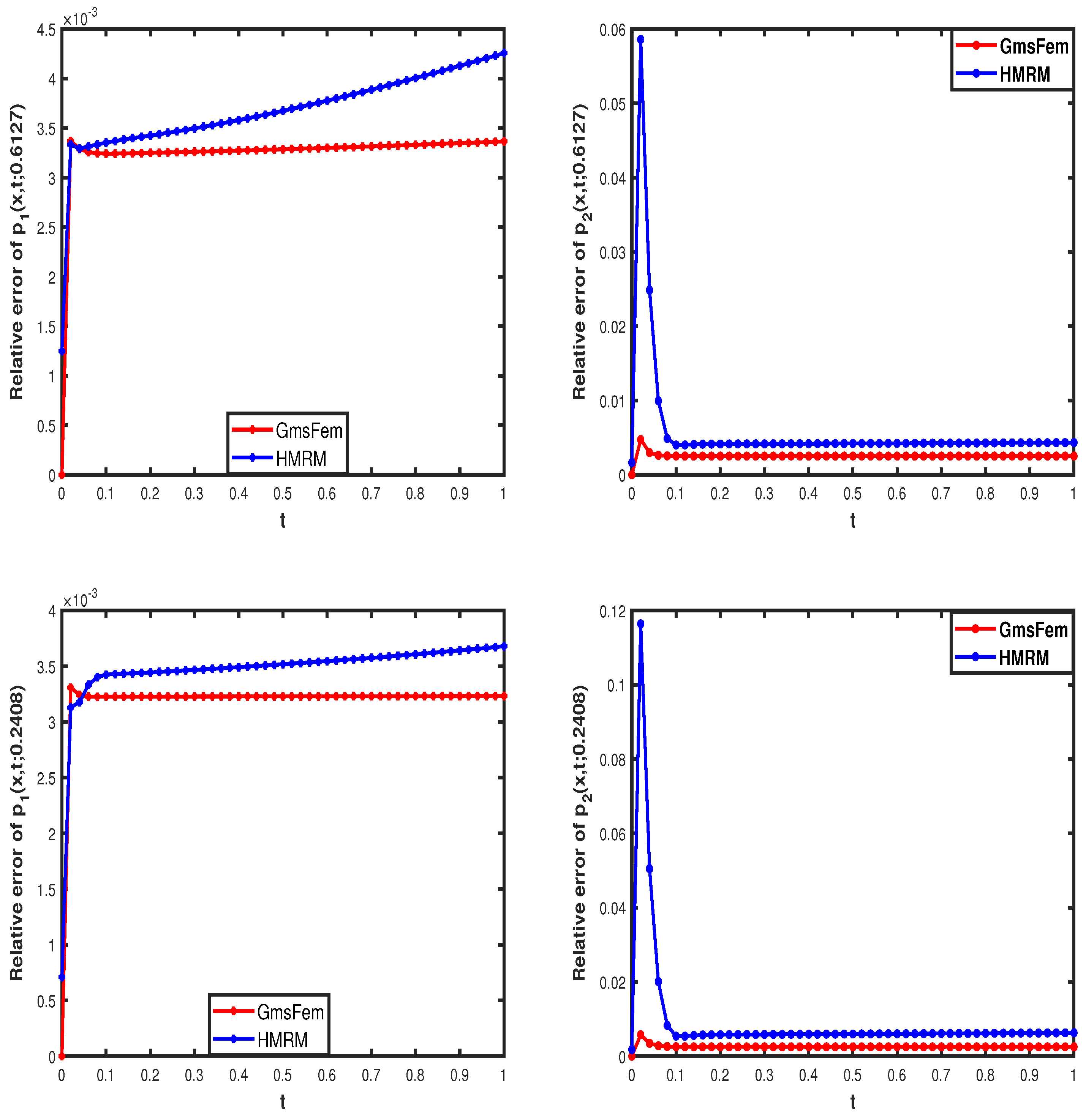
To evaluate the performance of the hybrid model reduction method, we compute the average relative error over an ensemble of 1000 randomly selected parameter samples.
The numerical setup is configured as follows: the number of local basis functions per coarse element is fixed at , and the number of variable-separation terms is also set to five. To systematically investigate the impact of the coarse mesh resolution on the approximation accuracy, we conduct a series of experiments with varying coarse mesh sizes, specifically .

Table 1.
The relative errors with different coarse mesh size H for and .
| 5.0389E-01 | 1.2556E-01 | 1.3176E-01 | 3.2681E-03 | 3.4457E-03 | 1.2881E-03 | |
| 5.0337E-01 | 1.2563E-01 | 1.3191E-01 | 4.6316E-03 | 4.1590E-02 | 5.9059E-03 | |
| 2.2118E-01 | 1.3833E-01 | 8.7244E-02 | 2.5336E-03 | 1.8137E-03 | 1.4234E-03 | |
| 2.2208E-01 | 1.4099E-01 | 8.6095E-02 | 7.0355E-03 | 8.9305E-03 | 5.4730E-03 |
Figure 4.
The average relative errors corresponding to the time t.
6.2. Experiment 2
In this subsection, we consider the dual-continuum with random inputs as follows.
where the diffusion coefficients, the transfer coefficient, and the source terms are defined by
Here and the random variable obeys the beta distribution, i.e., . and are both high-contrast functions independent of , whose maps are depicted in Figure 5.
The conductivity values in the background both are fixed to be 1, while the conductivity values in the channels are 10000. In this experiment, we randomly take 2000 random samples to test the proposed iterative method. The boundary conditions and initial condition are set as
respectively. In this experiment, the solutions of the multi-continuum model for the three methods: FEM on fine grid (reference solutions), GMsFEM on coarse mesh size and the proposed model reduction method.
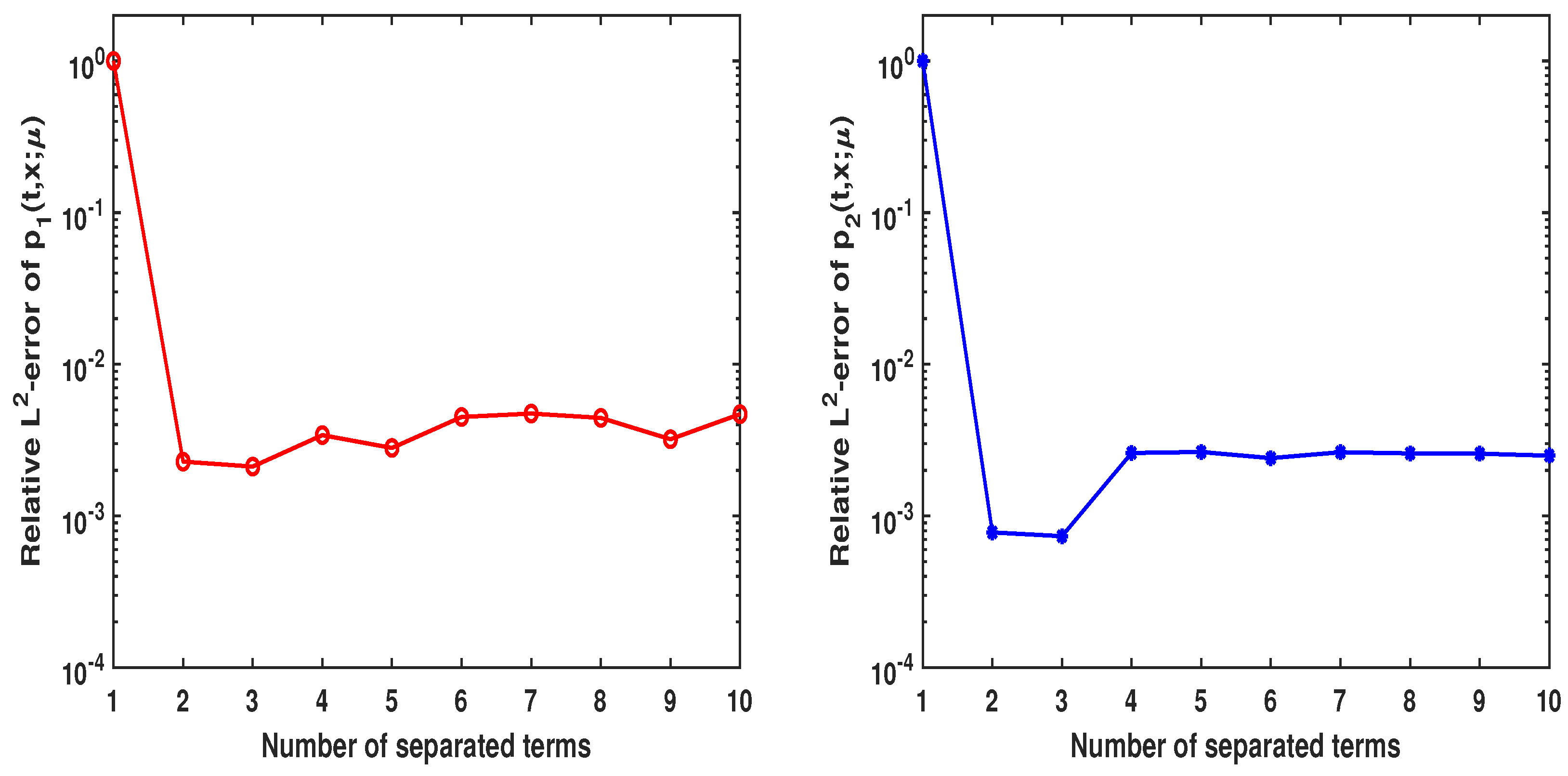
To evaluate the approximation accuracy for the hybrid model reduction method, we randomly selected 2000 parameter samples and compute the average relative -errors. Using a fixed number of separated terms () and five local basis functions in GMsFEM, the mean and the variance of variables and are illustrated at a random time layer in Figure 6 and Figure 7, respectively.
The figure demonstrates that the solutions for both and closely match their respective reference solutions.
To systematically assess the impact of the coarse mesh resolution on accuracy, we conduct experiments using progressively refined meshes with sizes . We compare the relative errors of all methods in Table 2.
These results, presented in the table, demonstrate that the approximation accuracy of both the hybrid method and GMsFEM improves—that is, their respective errors decrease—as the coarse mesh is refined.
Figure 7.
The variance of (1st row) and (2nd row) by different methods.
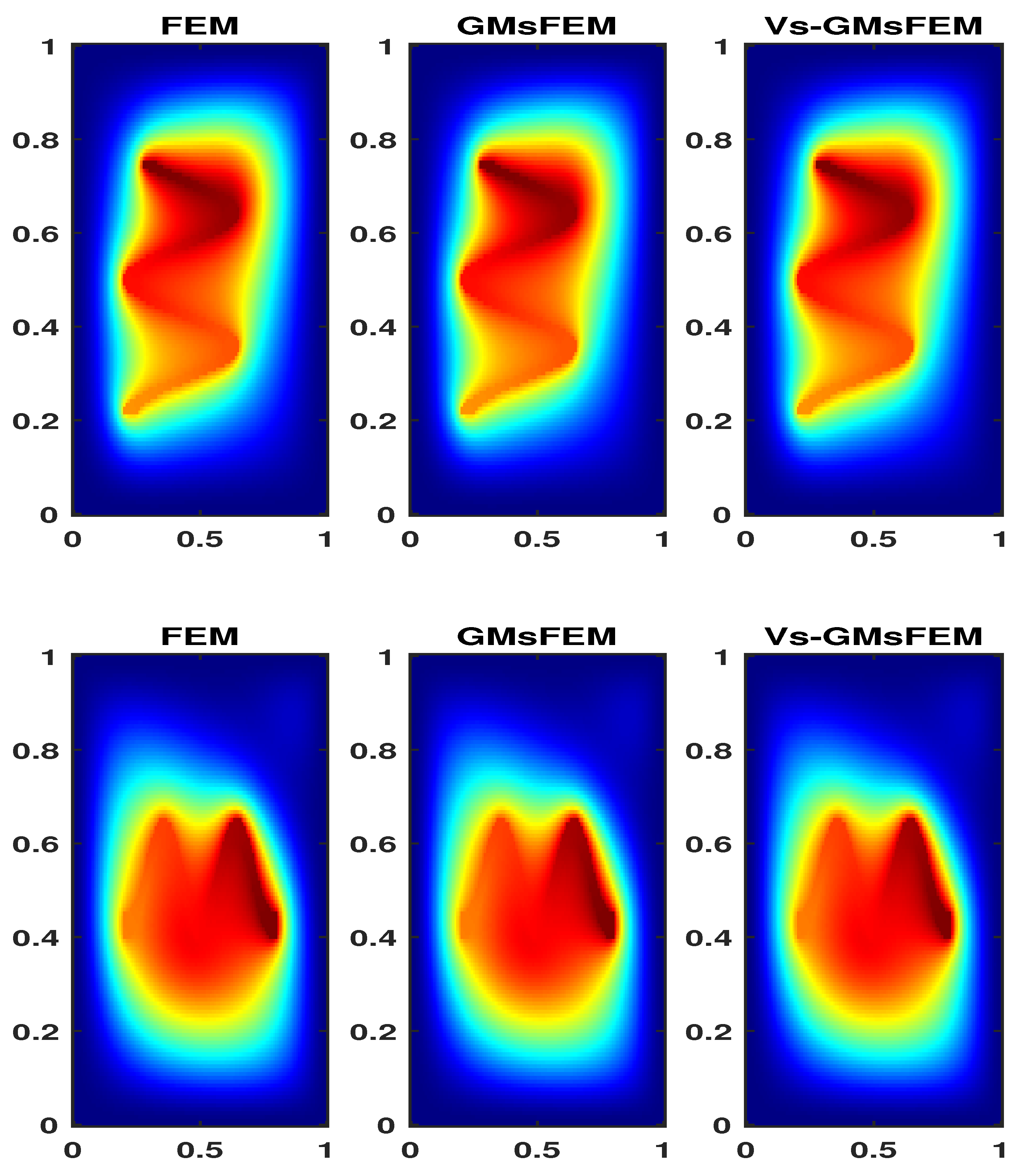
Figure 8.
The relative -error of numerical solutions: (left) and (right) with different number of separated terms.
Figure 8.
The relative -error of numerical solutions: (left) and (right) with different number of separated terms.
7. Conclusions
In this paper, we present a hybrid model reduction method for solving stochastic dual-continuum models. In this work, In this work, the possible uncertainties considered originate in the PDE coefficient, the transfer term, and the source term. Directly solving these equations on a fine grid presents a significant computational challenge, particularly in many-query scenarios. To dramatically improve efficiency, our method integrates the uncoupled Generalized Multiscale Finite Element Method (GMsFEM) with a low-rank variable-separation technique to construct compact representations of the solutions. This hybrid approach enables the computation of a large number of stochastic realizations at minimal cost. In the numerical experiments section, we apply the proposed model reduction method to dual-continuum models with random inputs. The results confirm that our hybrid method achieves an effective trade-off between computational efficiency and accuracy.
Acknowledgments
This work was supported by the National Natural Science Foundation of China (Grant No. 12101217) and by the Natural Science Foundation of Hunan Province (Grant No. 2022JJ40113).
Appendix A Online-Offline Computation of Residuals
By affine representations (3) and definition of residuals, we can express the residuals as
By (13) and the above expressions about residuals, we can get
This implies that
where is the Riesz representation of , i.e., for any . is the Riesz representation of , i.e., for any . is the Riesz representation of , i.e., for any , where . is the Riesz representation of , i.e., for any , where and . is the Riesz representation of , i.e., for any , where and . is the Riesz representation of , i.e., for any , where , .
Eq. (A.25) gives rise to
and
References
- Arbogast, T.; Douglas, J.; Hornung, U. Derivation of the double porosity model of single phase flow via homogenization theory. SIAM J. Math. Anal. 1990, 21, 823–836. [Google Scholar] [CrossRef]
- Akkutlu, I.; Efendiev, Y.; Vasilyeva, M.; Wang, Y. Multiscale model reduction for shale gas transport in a coupled discrete fracture and dual-continuum porous media. J. Nat. Gas Sci. Eng. 2017, 48, 65–76. [Google Scholar] [CrossRef]
- Barrault, M.; Maday, Y.; Nguyen, N.; Patera, A. An empirical interpolation method: application to efficient reduced-basis discretization of partial differential equations. C. R. Math. Acad. Sci. Paris 2004, 339, 667–672. [Google Scholar] [CrossRef]
- Barenblatt, G.; Zheltov, I.; Kochina, I. Basic concepts in the theory of seepage of homogeneous liquids in fissured rocks [strata]. J. Appl. Math. Mech. 1960, 24, 1286–1303. [Google Scholar] [CrossRef]
- Cheung, S.; Chung, E.; Efendiev, Y.; Leung, W.; Vasilyeva, M. Constraint energy minimizing generalized multiscale finite element method for dual continuum model. arXiv e-prints 2018, arXiv:1807.10955. [Google Scholar] [CrossRef]
- Chung, E.; Efendiev, Y.; Leung, W. Constraint energy minimizing generalized multiscale finite element method. Comput. Methods Appl. Mech. Engrg 2018, 339, 298–319. [Google Scholar] [CrossRef]
- Chung, E.; Efendiev, Y.; Leung, W. Fast online generalized multiscale finite element method using constraint energy minimization. J. Comput. Phys. 2018, 355, 450–463. [Google Scholar] [CrossRef]
- Chung, E.; Efendiev, Y.; Leung, W.; Vasilyeva, M.; Wang, Y. Non-local multi-continua upscaling for flows in heterogeneous fractured media. J. Comput. Phys. 2018, 372, 22–34. [Google Scholar] [CrossRef]
- Bogdanov, I.; Mourzenko, V.; Thovert, J.; Adler, P. Two-phase flow through fractured porous media. Phys. Rev. E 2003, 68, 026703. [Google Scholar] [CrossRef] [PubMed]
- Li, Q.; Jiang, L. A novel variable-separation method based on sparse and low rank representation for stochastic partial differential equations. SIAM J. Sci. Comput. 2017, 39, A2879–A2910. [Google Scholar] [CrossRef]
- Eikemo, B.; Lie, K.; Eigestad, G.; Dahle, H. Discontinuous Galerkin methods for advective transport in single-continuum models of fractured media. Adv. in Water Res. 2009, 32, 493–506. [Google Scholar] [CrossRef]
- Efendiev, Y.; Hou, T.Y. Multiscale Finite Element Methods. Theory and Applications; Springer-Verlag New York, 2009. [Google Scholar]
- Efendiev, Y.; Hou, T.; Ginting, V. Multiscale finite element methods for nonlinear problems and their applications. Commun. Math. Sci. 2004, 2, 553–589. [Google Scholar] [CrossRef]
- Efendiev, Y.; Galvis, J.; Hou, T. Generalized multiscale finite element methods (GMsFEM). J. Comput. Phys. 2013, 251, 116–135. [Google Scholar] [CrossRef]
- Erhel, J.; de Dreuzy, J.R.; Poirriez, B. Flow simulation in three-dimensional discrete fracture networks. SIAM J. Sci. Comput. 2009, 31, 2688–2705. [Google Scholar] [CrossRef]
- Evans, L. Partial differential equations, 2nd. ed.; Amer. Math. Soc, 1998. [Google Scholar]
- Fu, S.; Chung, E.; Mai, T. Constraint energy minimizing generalized multiscale finite element method for nonlinear poroelasticity and elasticity. J. Pet. Sci. Eng. 2020, 417, 109569. [Google Scholar] [CrossRef]
- Granet, S.; Fabrie, P.; Lemonnier, P.; Quintard, M. A two-phase flow simulation of a fractured reservoir using a new fissure element method. J. Pet. Sci. Eng. 2001, 32, 35–52. [Google Scholar] [CrossRef]
- Grepl, M.; Maday, Y.; Nguyen, N.; Patera, A. Efficient reduced-basis treatment of nonaffine and nonlinear partial differential equations. ESAIM: Model. Math. Anal. Numer. 2007, 41, 575–605. [Google Scholar] [CrossRef]
- Geiger, S.; Matthäi, S.; Niessner, J.; Helmig, R. Black-Oil simulations for three-component, three-phase flow in fractured porous media. SPE Journal 2009, 14, 338–354. [Google Scholar] [CrossRef]
- Kalachikova, U.; Ammosov, D. Advancing wave equation analysis in dual-continuum systems: A partial learning approach with discrete empirical interpolation and deep neural networks. J. Comput. Appl. Math. 2024, 443, 115755. [Google Scholar] [CrossRef]
- Jiang, L.; Li, Q. Reduced multiscale finite element basis methods for elliptic PDEs with parameterized inputs. J. Comput. Appl. Math. 2016, 301, 101–120. [Google Scholar] [CrossRef]
- Li, Q.; Wang, Y.; Maria, V. Multiscale model reduction for fluid infiltration simulation through dual-continuum porous media with localized uncertainties. J. Comput. Appl. Math. 2018, 336, 127–146. [Google Scholar] [CrossRef]
- Matthäi, S.; Mezentsev, A.; Belayneh, M. Finite element-node-centered finite-volume two-phase-flow experiments with fractured rock represented by unstructured hybrid-element meshes. SPE Reserv. Eval. Eng. 2007, 10, 740–756. [Google Scholar] [CrossRef]
- Modesto, D.; Zlotnik, S.; Huerta, A. Proper generalized decomposition for parameterized helmholtz problems in heterogeneous and unbounded domains: application to harbor agitation. Comput. Methods Appl. Mech. Engrg 2015, 295, 127–149. [Google Scholar] [CrossRef]
- Nouy, A. Recent developments in spectral stochastic methods for the numerical solution of stochastic partial differential equations. Arch. Comput. Methods Eng. 2009, 16, 251–285. [Google Scholar] [CrossRef]
- Nouy, A.; Maitre, O. Generalized spectral decomposition for stochastic nonlinear problems. J. Comput. Phys. 2009, 228, 202–235. [Google Scholar] [CrossRef]
- Nouy, A. Proper generalized decompositions and separated representations for the numerical solution of high dimensional stochastic problems. Arch. Comput. Methods Eng. 2010, 17, 403–434. [Google Scholar] [CrossRef]
- Pacciarini, P.; Rozza, G. Stabilized reduced basis method for parametrized advection– diffusion PDEs. Comput. Methods Appl. Mech. Engrg 2014, 274, 1–18. [Google Scholar] [CrossRef]
- Quarteroni, A.; Manzoni, A.; Negri, F. Reduced basis methods for partial differential equations; Springer: New York, 2015. [Google Scholar]
- Rozza, G.; Huynh, D.; Patera, A. Reduced basis approximation and a posteriori error estimation for affinely parametrized elliptic coercive partial differential equations. Arch. Comput. Methods Eng. 2008, 15, 229–275. [Google Scholar] [CrossRef]
- Vasilyeva, M.; Chung, E.; Cheung, S.; Wang, Y.; Prokopev, G. Nonlocal multicontinua upscaling for multicontinua flow problems in fractured porous media. J. Comput. Appl. Math. 2019, 355, 258–267. [Google Scholar] [CrossRef]
- Wu, Y.; Pruess, K. A multiple-porosity method for simulation of naturally fractured petroleum reservoirs. SPE Reservoir Engineering 1988, 3, 327–336. [Google Scholar]
- Yan, B.; Alfi, M.; Cheng, A.; Cao, Y.; Wang, Y.; Killough, J.E. General Multi-Porosity simulation for fractured reservoir modeling. J. Nat. Gas Sci. Eng. 2016, 33, 777–791. [Google Scholar] [CrossRef]
Figure 1.
The fine grid, coarse grid and the coarse neighborhood of node .
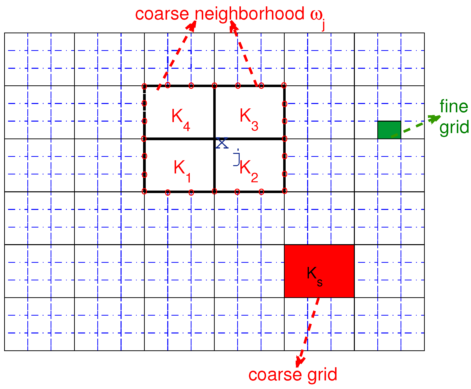
Figure 2.
High-contrast functions (left) and (right).
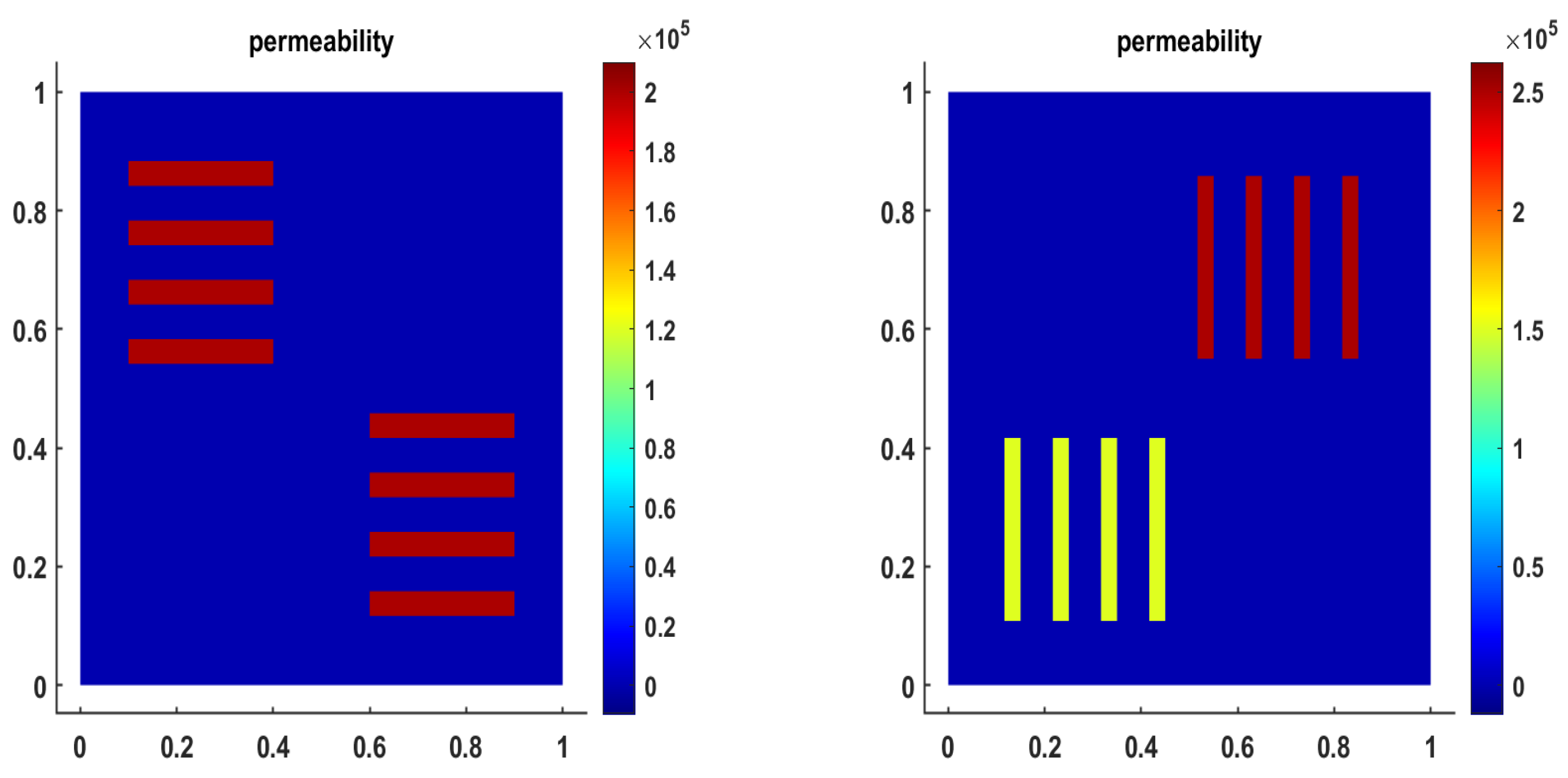
Figure 3.
Figures of (1st row) and (2nd row) by different methods.
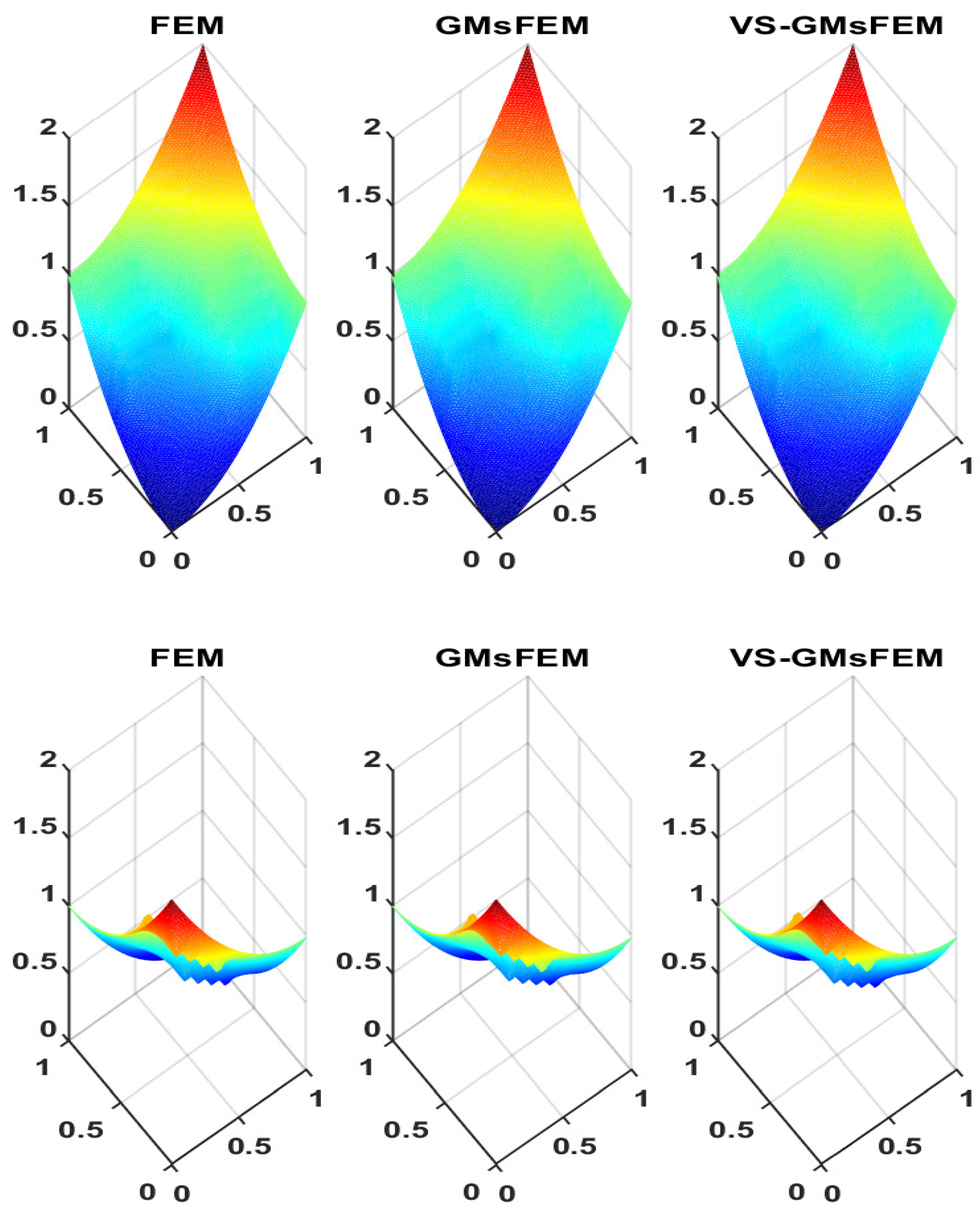
Figure 5.
High-contrast functions (left) and (right).
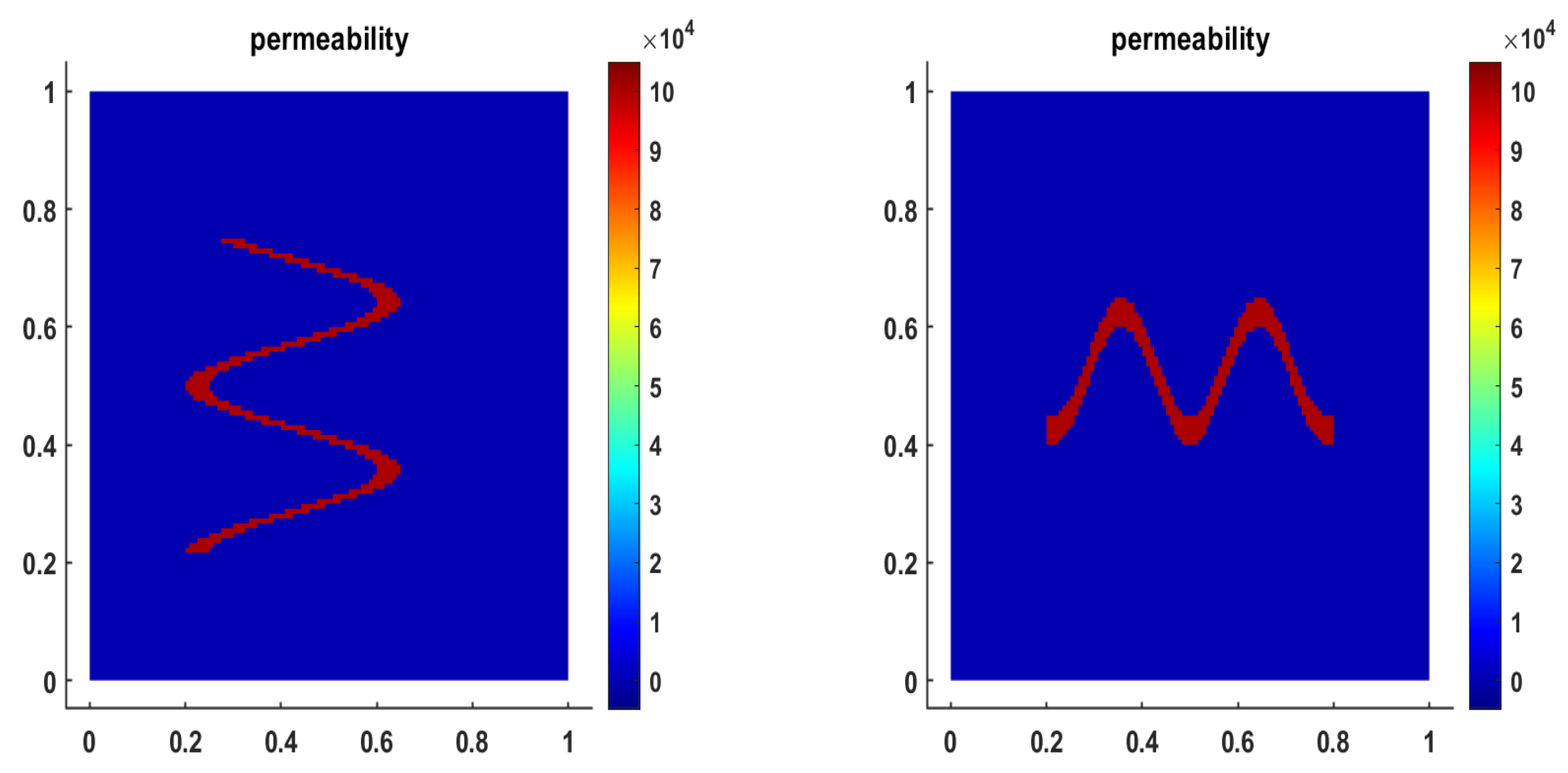
Figure 6.
The mean of (1st row) and (2nd row) by different methods.
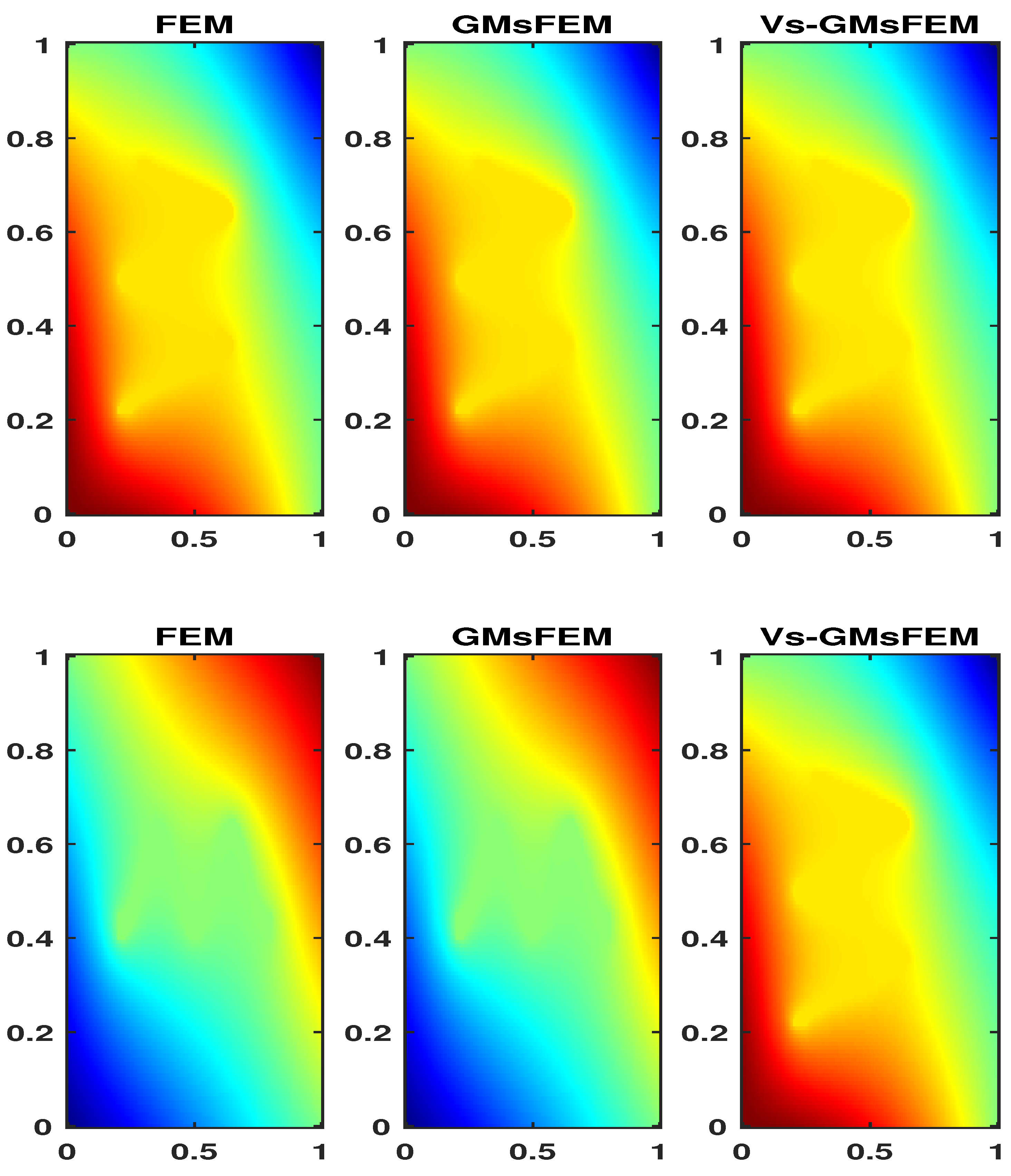
Table 2.
The relative errors with different coarse mesh size H for and .
| 1.8958E-01 | 1.7748E-01 | 2.0568E-03 | 1.2338E-03 | 5.3932E-04 | |
| 1.9047E-01 | 1.7539E-01 | 4.2623E-03 | 1.4946E-02 | 9.2871E-03 | |
| 1.7631E-03 | 1.9731E-03 | 3.5753E-03 | 1.4759E-02 | 9.2977E-03 | |
| 2.1234E-01 | 1.8409E-02 | 6.5206E-04 | 3.7393E-04 | 1.4397E-04 | |
| 2.1175E-01 | 1.8218E-02 | 1.4602E-03 | 2.0708E-03 | 1.4111E-03 | |
| 9.7625E-04 | 5.3918E-04 | 1.3870E-03 | 2.0860E-03 | 1.3949E-03 |
Disclaimer/Publisher’s Note: The statements, opinions and data contained in all publications are solely those of the individual author(s) and contributor(s) and not of MDPI and/or the editor(s). MDPI and/or the editor(s) disclaim responsibility for any injury to people or property resulting from any ideas, methods, instructions or products referred to in the content. |
© 2026 by the authors. Licensee MDPI, Basel, Switzerland. This article is an open access article distributed under the terms and conditions of the Creative Commons Attribution (CC BY) license (http://creativecommons.org/licenses/by/4.0/).
Copyright: This open access article is published under a Creative Commons CC BY 4.0 license, which permit the free download, distribution, and reuse, provided that the author and preprint are cited in any reuse.


