
Submitted:
28 January 2026
Posted:
29 January 2026
You are already at the latest version
Abstract
Dynamic beam shaping enables completely new possibilities for improving applications in laser material processing. This involves introducing numerous time constants and fre-quencies that must be set correctly to successfully modify a specific process. The present paper proposes consistent naming of the possible types of dynamic beam shaping and the resulting dynamic process modifications in relation to characteristic time constants and frequencies. The characteristic frequencies define three distinct process regimens that can be related to successful process modifications such as the reducing of pores. An overview of typical time constants and frequencies associated with laser processes is given, to ease the determination of characteristic frequencies involved in beam shaping with DBLs. The knowledge of the process regimes provides a guide to systematically assess suitable beam shaping parameters for specific dynamic process modifications to e.g. control issues such as pores, spiking, or spattering. An example demonstrating the reduction of process pores confirming these findings is included.
Keywords:
laser processing
; laser applications
; solving laser process issues
; dynamic beam shaping
; dynamic process modifications
; dynamic beam lasers (DBL)
1. Introduction
The processing of a wide range of materials using continuous-wave lasers is well established in industrial manufacturing. Key processes include hardening, where the material remains in the solid state; cutting, where the material is melted; and deep-penetration welding, where partial vaporization occurs. These processes enable a broad spectrum of industrial applications as is extensively described for example in [1].
In recent years, significant progress has been made in both laser technology and industrial applications. On the one hand, the average power of commercially available solid-state lasers has increased significantly - from a few kilowatts in 2005 to over 100 kW by 2022 [2]. On the other hand, the development of novel materials and enhanced processing techniques has paved the way for new applications. These include current progress in different industries like the use of high-strength alloys in crash boxes, aluminum-copper combinations for high-current applications such as in locomotives, and large-scale applications driven by the automotive industry's transition to e-mobility – such as welding large aluminum cooling plates and copper hairpins. Moreover, the trend toward mass individualization has led to a resurgence of laser-based additive manufacturing, ranging from powder- and wire-based material deposition (DED) to powder bed fusion by a laser beam (PBF-LB).
All these applications involve specific challenges regarding process stability and the resulting quality. Key issues include minimizing striations and dross, controlling kerf angles during the cutting of thick materials, and avoiding pores, spattering, humping, and the formation of hot cracks in the solidifying material during high-speed welding.
A promising approach to address these challenges is the active forming of the intensity distribution in the focused laser beam, usually referred to as beam shaping. The beam’s intensity profile has a key influence on the energy deposition in the workpiece and therefore on the entire process. The irradiance distribution resulting from the beam shape and the geometry of the interaction zone on the workpiece can be used to modify process features such as widening a weld seam, influencing the heat flow or enlarging a keyhole. Illustrative examples for deep-penetration laser welding are given in [3,4,5]. Theoretical modelling confirmed the influence of shaped beams on the shape of the welding keyhole [6,7]. As a result, various beam shaping methods have been developed and are successfully applied to improve different aspects of the laser welding process [8,9,10,11,12,13,14]. These beam shaping systems range from static configurations to dynamic systems operating at low modulation frequencies. Comprehensive overviews of beam shaping techniques can be found in [15,16].
Dynamic beam shaping is particularly comprehensive with lasers that enable very fast creation of arbitrary beam shapes. This can be implemented by means of actively controlled coherent beam combining. Current lasers based on this principle, referred to as “dynamic beam lasers” (DBLs), allow to create the time-averaged beam shapes by quickly scanning a single intensity peak to different positions in the focal plane at frequencies of up to 80 MHz. This method enables the generation of arbitrarily time-average beam shapes composed of a sequence of points on the workpiece surface that are scanned by an intensity peak in rapid succession, even at average powers exceeding 100 kW [17]. The time-average beam shapes themselves can be changed with frequencies in the order of MHz, offering unprecedented potential for influencing and controlling laser material processing, as first demonstrated in [18]. Offering such fast dynamic beam shaping, DBLs introduce additional time constants and frequencies into beam shaping, such as the dwell time of the intensity peak at a single position or refresh frequency of the time-average beam shape, which increases complexity but also opens a wide range of new possibilities for process control or process modifications.
Laser processing with dynamically modulated process parameters have revealed that characteristic modulation frequencies exist at which the influence on the process is particularly strong as e.g. seen in [19], where power modulation with about 300 Hz significantly improved welding of copper at the given process parameters. The knowledge of such characteristic frequencies is very helpful to allow deterministic process modification. At the present state of knowledge, it may be assumed that these characteristic frequencies are related to typical time constants and frequencies of the process.
The paper also proposes consistent naming of the possible types of beam shaping and process modifications and sets them in relation to characteristic time constants and frequencies. The characteristic frequencies allow to define three distinct process regimens, which can be related to successful process modifications such as the reducing of pores, giving hand to deterministic process development. An overview of typical time constants and frequencies associated with laser processes is given, to ease the determination of characteristic frequencies involved in beam shaping with DBLs.
The knowledge of the process regimes provides the basis for a guide to systematically assess suitable beam shaping parameters for specific dynamic process modifications to e.g. control issues such as pores, spiking, or spattering. An example demonstrating the reduction of process pores confirming these propositions is included.
2. Typical Time Constants and Frequencies in Laser Processes
Duration for Spreading the Heat
The depth of hardening or the thickness of the liquid layer between the welding keyhole and the solid material is given by the location or the distance between the respective isotherms. The thermal diffusion length
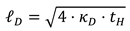 is commonly considered as a measure of the spatial extent of the temperature increase [1], where is the thermal diffusion constant, the heat conductivity, ρ the mass density and cp the specific heat capacity at constant pressure for the phase considered, and tH is the duration of heating. A few values for κD for a selection of common metals can be found in [22,23] and are summarized in Error! Reference source not found. in the Appendix A. Solving for tH gives the time
 it takes until the temperature increase of about 9%.Tmax reaches the extent ℓD, where Tmax is the maximum temperature reached after the duration on the surface, which is heated by the laser radiation.
Example: In solid iron, with κD,Fe = 2.3.10-5 m2/s, the time for reaching about 9%.Tmax at the distance of 0.5 mm below the irradiated surface is about 2.8 ms, whereas in solid aluminum, with κD,Alu = 9.8.10-5 m2/s, this time is only about 640 µs.
If the influence of heat conduction should be neglectable, the thermal diffusion length must be smaller than any critical extent ℓC of heat affected zones, such as melt layers, length of cracks or extents of hardened areas, i.e. ℓD < ℓC which means that the heating duration tD must fulfil the condition

Duration for Reaching a Specific Temperature
The time required to heat the material to its melting or boiling temperature using a laser beam is of interest in every laser process. A convenient analytical approximation to estimate the temperature increase , where is the initial temperature, can be found e.g. in [1] with the assumptions of heating the surface of a semi-infinite body. For short heating times tH and hence one-dimensional heat flow induced by a Gaussian beam at normal incidence, the temperature increase on the surface is given by
where 𝜅T = 𝜌 · cp · λth, is the beam diameter on the workpiece surface, the laser power and the absorptivity of the material at the wavelength of the laser beam. A few values for κH for a selection of common metals are summarized in Error! Reference source not found..
The duration tH for reaching a target temperature when starting from a given initial temperature on the surface of a material is therefore given by
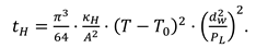
Examples: In aluminum in liquid state at the melting temperature of T0 = 660°C, with κH = 2.9.108 J2/m4/s/K2, (material values are taken for the liquid phase), the time for reaching evaporation temperature of T =Tv = 2520°C on the surface when heating with a laser beam of 0.5 mm diameter, an average laser power of 10 kW and taking an absorptivity of A = 6% is about 167 µs. In contrast, in iron with κH = 2.3.10-5 m2/s and A = 40% the time is about 0.9 µs which is about 185x faster.
Propagation of Acoustic Excitations
The time for an acoustic excitation in the liquid metal to travel the distance of the laser beam diameter on the workpiece is given by
where is the velocity of sound, the values of which in liquid metals can be found in [24]. A few values for a selection of frequently used metals are summarized in Table 5.
Examples: The time for an acoustic excitation to travel the distance of the diameter of the laser beam is about the same in aluminum and iron tS = 0.1 ms. It is noted that, for example in deep-penetration laser welding, the melt pool is much longer in steel than in aluminum and strongly depends on the processing parameters and beam shapes. Therefore, the time for an acoustic excitation to reach the solidification region must be calculated for each process parameter set.
Maximum Flow Speed Around a Keyhole
If a keyhole exists e.g. during laser welding, the melt created in front of the keyhole must flow around the keyhole. The maximum velocity of this melt flow is one of the important quantities defining the quality of the weld as was described in the introduction. The speed of the flow of the liquid metal around the keyhole was described in the PhD-work of Beck at the IFSW [23]. A comprehensive summary of the work can be found in [1] p. 325ff. For a cylindrical keyhole with a diameter of the diameter of the laser beam and assuming that the velocity of the liquid metal vL increases linearly from the border of the melt pool to the border of the keyhole, the maximum flow velocity vL,max can be approximated by [23]
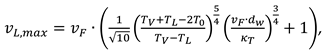 where vF is the feed rate, the melting temperature, the vaporization temperature, and the initial temperature. It is seen that for low feed rates and small beam diameters , whereas for very high feed rates, the maximum flow velocity scales with about . However, as the width of the liquid layer in eq. (7) is purely determined by heat conduction, it is possible to influence the maximum flow speed by increasing the difference between the lateral width of the melt pool and the lateral keyhole width, e.g. with modified laser beam profiles or beam wobbling.
The time for the liquid to pass the keyhole, within which it is possible to influence the melt flow with the laser beam, can be calculated with
Figure 1 shows for example the minimum liquid-keyhole-passing-time as a function of the feed rate for aluminum (blue) and iron (orange) for a beam diameter of 0.5 mm and the material values κT,Al = 9.8.10-5 m2/s and κT,Fe = 2.3.10-5 m2/s.
At the feed rate of 6 m/min the keyhole-passing-time for aluminum is about 10 ms and for steel 3 ms. At the feed rate of 60 m/min the keyhole-passing-time for aluminum is reduced to about 200 µs and for steel to 80 µs.
Keyhole Collapse, Pore Formation and Spiking
Partial or complete keyhole collapse is the origin of several issues such as blow outs, pore formation or spiking at the tip of the keyhole [1]. The keyhole collapse shows typical time constants tc and quasi-periodicity with the frequency fc = 1/tc which depends on the process parameters and the processed material. The time constants of the process are determined by convection and surface tension and rates of vaporization inside the keyhole which determine how long it takes to open or close a capillary. Convenient analytical solutions do not exist to the best of our knowledge. However, recent publications allow estimations of the time constants involved: Opening and closing time of a keyhole in steel was seen is in the order of tc = 1 ms [18]. In [18] it was observed in deep-penetration welding of steel that the tip of the capillary could clearly follow the movement of a laser beam up to frequencies of fc = 100 Hz, i.e., within about tc = 10 ms, while no clear correlation to the excitation was found for frequencies of fProc = 1 kHz and higher. In [26] it was measured in Ti that the collapse at the tip of the keyhole, which might result in the formation of a pore, happened in about tc = 4 µs.
Summary of the Examples for Typical Time Constants and Frequencies
Table 1 shows a summary of a few typical process time constants for the physical quantities given above for a feed rate of 1 m/s and an average laser power of 10 kW. For the corresponding frequencies, a periodic repetition of the effect was assumed.
A thermal diffusion length of ℓD = 0.5 mm and a width of the laser beam on the surface of dW =0.5 mm were taken as typical values for the example. It is seen that the frequency range spreads over more than three orders of magnitude, from the lowest frequencies in the range of 1 kHz up to the highest frequency of 1 MHz. It can be assumed that characteristic frequencies of beam shaping are expected in this range. However, due to the strong dependence on the processing parameters and on the material properties, the values must be determined for each specific configuration.
Beam Shaping to Modify the Process: Basic Definitions
Beam shaping generally refers to any temporal and spatial manipulation of the beam shape, i.e. the laser beam’s spatio-temporal intensity distribution and its polarization. This begins within the laser resonator, where the beam is generated as a superposition of resonator modes. Temporal properties such as repetition rate and pulse shape are defined by techniques like mode locking or Q-switching. Extra cavity spatial beam shaping includes all approaches reviewed in [15,16], as well as power modulation and pulse stretching or compression. Hence, beam shaping – as the term implies – refers solely to the manipulation of the beam itself.
The primary goal in laser applications, however, is not merely to shape the beam, but to achieve process modifications that enhance process quality and productivity. The actual impact on the process is governed by the irradiance distribution and the polarization on the surface of the workpiece. In the simplest case of a beam incident on a flat surface, the irradiance is given by J(x,y,z,t) = cos(𝜑)I(x,y,z,t), where φ is the angle of incidence and the intensity distribution in in the cross section of the beam. In most practical scenarios, however, the irradiance at the workpiece – and therefore the spatio-temporal distribution of the absorbed power density – is influenced by the geometry of the interaction zone and by multiple reflections therein. The geometry might change dynamically leading to a time-dependent absorbed power density. As a result, the absorbed irradiance is determined by both the beam shaping and the process conditions, and these two aspects cannot be considered independently. This means that the process modifications cannot be directly related to the beam shapes making deterministic process design very challenging.
In the following, consistent terms involved in “beam shaping”, “dynamic beam shaping” and the resulting process modifications are proposed in view of their temporal characteristics. The aim is to suggest a general convention for a nomenclature to facilitate comparison across the wide range of methods that use beam shaping to influence laser processes and to enable an unambiguous exchange also between different disciplines like optics, systems engineering, materials processing, or manufacturing.
For the case of laser materials processing considered here, the process parameters are referred to as in the following. This includes quantities such as e.g. material properties, feed rate, laser power, focus position, and irradiance distribution. For easier distinction, process parameters related to beam shaping are referred to as .
In contrast refers to all process features such as e.g. width and depth of a weld seam, diameter and depth of a keyhole, width of a heat affected zone, velocity of the melt flow, spattering, and pore formation. In practice, the process parameters are optimized and adjusted to achieve specific desired process features which are optimal for a specific application. In the following, the considerations are focused on the process itself, i.e., we consider the interaction zone through which the material moves depending on the feed rate. This perspective aligns with the energy, momentum, and force balances that govern process stability.
Static Process Modifications
Most laser-based processes achieve optimum quality when operating in a form of dynamic steady state. In the simplest case, this state is achieved with static process modifications, i.e., time-invariant process parameters with . This includes, for example, a constant relative velocity between the laser beam and the workpiece along a linear path, where . A steady state can also be maintained during motion along a circular path, provided the relative speed remains constant. In this case, , while due to the continuous change in direction. In both scenarios, the absence of wobbling is essential for maintaining a constant absolute value of the speed.
Static beam shaping therefore refers to measures that aim at adjusting the intensity distribution and the polarization of a beam permanently and constantly, i.e., with no temporal change, with the goal to reach static process modifications, which optimize the specific process features. This is e.g. reported in [4], where the process features spatters and pores are minimized with superimposed laser beams. In [20] a beam with a core and ring profile enabled smooth and pore-free deep penetration welds with a subsequent wire filling process in brass. In [21] a mm-wide annular beam shape enabled control of the melt pool to reduce process defects.
Dynamic Process Modifications
The term “dynamic process modification” in the following refers to methods in which one or more process parameters vary over time. This is characterized by and/or . The variation of the process parameters might occur during the modulation time or with the modulation frequency .
Characteristic Time Constants and Characteristic Frequencies
Laser processing with varying process parameters during a time in a non-periodic manner is state of the art for example in laser cutting, where usually the average laser power is adapted to the current feed rate at the beginning of a cut or during cutting of corners to keep the line energy constant. The duration, over which the laser power is decreased or increased, is adapted to the geometry of the cut, the feed rate and the acceleration. Further examples are adaptation of the focal position and the laser power to changes in the thickness of the material. Such parameter modulations have characteristic time constants, which are given by properties of the processing system, the material properties of the processed sample and properties of the process itself.
The focus in this paper is on periodic parameter changes with frequencies that are inherent to DBLs. It is seen that with periodic parameter changes characteristic modulation frequencies exist, at which the influence on the process is particularly strong as described in the introduction. More generally speaking, it is observed that some of the features of a process are sensitive to the frequency of periodic changes of specific process parameters , i.e. that a process feature undergoes pronounced changes when a process parameter is modulated at a certain characteristic frequency , where takes into account, that there may be several different frequencies at which the process feature is sensitive to a modulation of . The types of dynamic process modifications are discussed in the following.
Non-Periodic Dynamic Process Modifications
With non-periodic process modifications, one or more parameters are changed as a function of time during the process, where is the duration of the non-periodic modification. The best process result is obtained when non-periodic dynamic process modifications are adapted to the characteristic time constants involved in the process as described in the previous section.
Periodic Dynamic Process Modifications
With periodic dynamic process modifications, one or more process parameters are changed in a periodic manner during the process, i.e. with the frequency . For periodic process modifications, it is therefore more expedient to use frequencies than times. It is noted that periodic process modifications are usually addressed when considering Civan's DBLs, which are used as an example in this paper. With these lasers, both the positioning of the beam within a shape and changing between shapes can be done with a selectable frequency. The parameter modifications, which are induced with this dynamic beam shaping, must be compared to the characteristic frequencies involved in the considered process. This comparison leads to the three distinct regimes discussed in the following.
Direct Periodic Process Modifications
When a process parameter is periodically changed with a frequency  that is much smaller than any of the characteristic process frequencies, the feature directly follows the variation of the parameter as the process at any time continuously but momentarily adopts the state that would be obtained with the current value of in a static process modification.
that is much smaller than any of the characteristic process frequencies, the feature directly follows the variation of the parameter as the process at any time continuously but momentarily adopts the state that would be obtained with the current value of in a static process modification.Characteristic Periodic Process Modifications
A process feature is subject to characteristic peculiarities when the modulation frequency of the process parameter lies within a more or less large range around the characteristic frequency defined above.
It is important to note that the modulation of process parameters with a characteristic frequency , may be at resonance with typical process frequencies, at which a given feature tends to respond with a disproportionally strong amplitude to the excitation, or at antiresonance, at which the response of a process feature is disproportionally small, or at any other frequency leading to a characteristic behavior. Depending on the damping, there is always a certain bandwidth around these frequencies within which the features respond in the characteristic manner. Knowledge of the characteristic process frequencies is therefore the key for a deterministic process modification.
Although this is the most challenging regime for process modifications, it has a large potential for inducing very strong modification of the process.
Quasi-Static Periodic Process Modifications
When the process parameter is periodically changed with a frequency 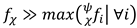 that is much higher than any of the characteristic frequencies, the process features cannot follow the immediate changes of the process parameters. Therefore, it will typically adopt a state that corresponds to the one obtained with a quasi-static value of that equals the time average of .
that is much higher than any of the characteristic frequencies, the process features cannot follow the immediate changes of the process parameters. Therefore, it will typically adopt a state that corresponds to the one obtained with a quasi-static value of that equals the time average of .Periodic Dynamic Beam Shaping
Periodic dynamic beam shaping refers to all beam shaping approaches that generate a periodic temporal change of the intensity and polarization distribution in the beam reaching the interaction zone of the process which lead to the periodic dynamic parameter modifications with the frequency fχB. This includes methods such as beam wobbling, periodic modulation of the average power, very fast repositioning of a laser beam on the surface to generate a time averaged intensity distribution, and periodic modulation of the beam shape as is of particular interest with DBLs. In this case the intensity distribution reaching the workpiece may be simultaneously characterized by several frequencies fχB related to different parameters involved in the dynamic beam shaping methods applied. These may include wobbling frequency, power modulation frequency, or the shape refresh and shape switch frequency of DBLs. It is important to emphasize that the term “dynamic” here refers to the way in which beam shaping is performed and is independent of the properties of the process. Whether periodic dynamic beam shaping acts as a direct, characteristic, or quasi-static dynamic process modification depends on the comparison with the characteristic frequencies as described above. The relations, which define the processing regimes, are summarized in Table 2.
To clearly distinguish between the regimes, the two operators “≪” and “≫” are recommended to denote at least a factor of five smaller and larger, respectively. Note that it is possible that a process is simultaneously influenced in different regimes of different parameters. To clarify the understanding of these definitions, an example based on the properties of Civan's Dynamic Beam Laser (DBL) is given in the following.
Summary of Properties and Frequency Definitions of DBLs
A very promising approach for periodic beam shaping to modify the process offer Civan's Dynamic Beam Lasers (DBLs) which allow process modifications in any of the regimes described in chapter 0. The basic properties of the current Civan-DBLs lasers are extensively described in [27] and summarized in the following to ease reading of this paper.
Properties of Points
Coherent combining of a bundle of fundamental mode fiber laser allows generating a plane overall phase front which results in a “point”, more precisely a diffraction pattern with a main lobe with high intensity, in the focal plane of a focusing lens. This main lobe contains up to 60% of the total laser power and is almost diffraction limited. The diameter of the main lobe depends on the focal length of the focusing lens. Figure 2(a) shows a false-color representation of the calculated, normalized intensity distribution for a main lobe created with a bundle of 36 fiber lasers, which is set in the center of the blue square (marked with the blue arrow). The color scale is shown on the right of Figure 2(a). The blue square represents the active area that contains >99.9% of the total laser power. Small side lobes to this main lobe appear in the active area, because the combined fibers represent a structure of a diffraction grating. By tilting the common phase front the point can be set at arbitrary positions (x,y) as shown in Figure 2(b). It is seen that the side lobes move with the main lobe and that the relative height of some of the peaks of the diffraction pattern are increased. The point can be set within the maximum positions (xmin,xmax) and (ymin,ymax), given by the position where the relative height of the main lobe and the three accompanying side lobes is the same as shown in Figure 2(c). The distance xmax- xmin = ymax- ymin = dS is referred to as scan width. The width of the blue active area is about 3x the width of the area within which the points can be set. The height of all lobes varies with the position in this area. Details are given in [27].
The following Table 3 lists typical values for the diameter of the main lobe, dML, the resulting maximum intensity for a 12 kW-laser, Imax,0,0, and the diameter of the active area, dActiveArea, for different focal lengths of the focusing lens fL.
It is noted that the maximum intensity is only reached when the point is set in the center of the active area with x = y = 0. At the positions (xmax,ymax), where the main lobe and the side lobes have the same height, the maximum intensity equals about 54% of Imax,0,0.
Sequencies of Points Create Shapes
The adjustment of the phases of the combined fibers is made with electro optic modulators (EOMs) in Civan's DBL. The EOMs are operated at a maximum frequency of fmax = 80 Mhz and therefore allow creating a common phase front and with it a point within tmin = 12.5 ns. This is a much shorter time constant than any encountered in laser processes as described in section 3. Therefore, it is possible to create arbitrary, quasi-static shapes composed by a very fast sequence of NSP points, which can be set at NPos arbitrary positions. A position of a point in the shape can be addressed more than once. On the one hand, this increases the total number of points in the shape, NSP. On the other hand, it increases the locally deposited energy compared to the other shape positions with less points per position. It is noted that increasing the number of points per position increases the fluence at this position but not the intensity.
The shape refresh frequency, i.e. the frequency with which the complete shape redrawn, fSR, can be chosen arbitrarily. This refresh frequency defines the point-frequency, which is given by fSP = fSR.NSP, with the boundary condition that fSP ≤ fmax. In fact, it is recommended to keep fSP smaller than about 50% of fmax to ensure clean build-up of each single point in the shape. Figure 3 shows a selection of quasi-static shapes. NSP equals the total number of the points in the shape.
Figure 3(a) shows a square with nine shape positions, NPos = 9. Each position was addressed with one single point once, therefore NSP = 9. Figure 3(b) shows the same square, with NPos = 9, but the central position (index i = 5) was addressed three times (nSP,i = 3) resulting in NSP = 11. The spiral and the hourglass shown in Figure 3(c) and (d), respectively, show the capability of DBLs to generate complex average shapes. These two shapes might be used for example to widen a keyhole because it generates a larger quasi-static shape, while the maximum intensity at each position in the shape remains almost constant, because the intensity of the points in the sequence does not change significantly in the active area. This allows keeping the intensity at each point high enough to stay above the deep penetration threshold [1].
Apart from creating single shapes, DBLs have the unique capability to switch between shapes, i.e. creating sequences of shapes. The switching can be done at very high frequencies, only limited by the condition fSP < fmax, which must hold for each shape in the sequence. Switching between the shapes can either be done periodically, with the shape duration frequency fSD, or non-periodically, where every shape in the shape sequence has its own shape duration. The latter case adds additional complexity to dynamic beam shaping and is not considered in the following.
The outstanding capability of switching shapes was demonstrated in several experiments: Triangles with opposite orientation have been used to demonstrate the completely different influence of the two shapes on the hydrodynamic behavior in liquid iron [30]. Switching between four points and a random point distribution have was used for demonstrating pore-free welding of copper hairpins in [28], and switching between a single point in the center of the active area and a curved line perpendicular to the feed direction allowed pore-free welding of mild steel as described in [29].
Furthermore, DBL-technology allows to actively shift the focus position in the direction of beam propagation by creating a parabolic common phase front. This can be also done in 12.5 ns enabling very fast shift of the focus. Details regarding shape sequencies and active focus shift (referred to as focus steering) are given in [27].
Deterministic Approach for Solutions to Process Issues Using DBLs
Dynamic beam lasers offer a virtually unlimited number of possibilities for process modification using fast beam shaping. Therefore, a deterministic approach to solutions to process issues using DBLs is highly recommended. In the following, a four-step approach is proposed to identify possible valid beam shapes and frequencies.
As an illustrative example the of emerging of process pores during welding of AlMgSi with an average laser power of 3.4 kW, a laser focus diameter of 680 µm, and a feed rate of 4 m/min will be used in the following to explain, how a deterministic approach could help to find solutions to process issues.
1st Step: Identify Possible Cause
The first step is to analyze possible mechanisms which cause the process issue. This requires basic understanding of how the process issues develop. The mechanism for the present, illustrative example is described in Figure 4 (a)-(e), which shows a sequence of five x-ray images taken out of an x-ray film with a total duration of about 250 µs. The x-ray film was recorded with a frame rate of 2 kHz. The green area with the dashed grey border marks regions with less density, i.e. the keyhole and in (d) and (e) in addition a bubble. It is seen in (a) that the starting point for the emergence of pores is a straight, narrow keyhole, which tends to bulge (b) and then constrict due to the fast vapor flow out of the keyhole (c) and the corresponding Bernoulli effect, which decreases the pressure in the upper part of the keyhole. Just before the collapse the tip of the keyhole is shaded, the vapor in the keyhole condensates on its surface resulting in a vacuum which sucks ambient air or process gas into the keyhole (c). After collapse (d) a gas-filled bubble remains which results in a pore when the material is solidified, and the narrow keyhole is built up again (e) finally re-starting with the straight, narrow keyhole (f).
For the parameters investigated here, the duration for a complete cycle is in the range of 15 ms yielding a characteristic frequency . The duration for bulging, constricting and separation of a bubble is about 2 ms yielding a characteristic frequency .
2nd Step Identify Possible Solutions
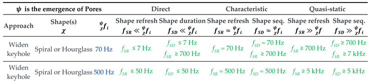
The second step is to evaluate possible approaches which allow to solve the issue. For the example of pore formation, the narrow keyhole seen in Figure 4 (a) and (e) is the starting point for the pore-formation cycle. Therefore, widening the keyhole and keeping it open is a promising approach for reducing the number of pores.
3rd Step: Identify Possible Beam Shapes and Rates
The use for example of a spiral or an hourglass as dynamic beam shape shown in Figure 3(c) and (d) is a straight-forward approach used in the following to illustrate the method. The maximum intensity in the beam must be chosen to exceed the deep penetration threshold for a moving beam as described in [1]. This is done by proper selection of the focal length of the focusing lens and the laser power. Furthermore, the diameter of the spiral must be chosen large enough to prevent bulging and constricting. The pictures in Figure 4 suggest that the diameter of keyhole at the entrance and therefore the diameter of the shape should be about three times larger than the diameter of the focus. Possible values for these beam parameters can be estimated from the numbers listed in Table 3 or calculated with the formula given in [27].
4th Step: Determine Frequency Domains and Their Process Response
The optimum temporal regime, i.e. the best values for the frequencies described in the previous section, is not obvious. On the one hand, it is not clear what of the three regimes given in Table 2 is most beneficial. On the other hand, the characteristic frequency for the envisaged process parameters and the processed material is usually not known. Therefore, it must be determined experimentally. In the present illustrative example, x-ray imaging allowed to determine two typical frequencies of 50 Hz and 500 Hz of the emergence of pores. It is noted that the x-ray film was taken with a frame rate of 2 kHz and therefore no effects with higher frequencies than this could be detected. The two frequencies are taken in the present example as a first approach to specify the decisive characteristic frequencies. A more practical example of how to determine characteristic frequencies is described in detail in the following chapter 0.
The Solutions Matrix
The four identification steps described in the preceding sections can be summarized in the “DBL solutions matrix” shown in Table 4, which uses the above example for reducing pores. The first two columns show the possible physical approach and promising shapes. The third column summarizes the characteristic frequencies . In the present example, the process feature is pores. For the process parameter , the dynamic beam shape is taken, which is refreshed with the characteristic frequency and . In the case of Civan's DBL lasers, each of the three regimes direct, characteristic and quasi-static as defined in Table 2 have to be considered for both, the shape refresh frequency fSR and the shape duration frequency fSD as defined in section 0. The green values in the table finally propose meaningful frequencies fSR and fSD for testing with the process. When changing the frequencies fSP ≤ fmax must be considered.
It is noted that the numbers in green result from the evaluation of the x-ray film, which does not allow considering frequencies larger than 1 KHz. However, these numbers may be taken as starting points for experimental investigations on how to reduce process pores during welding of AlMgSi with an average laser power of 3.4 kW, a laser focus diameter of 680 µm, and a feed rate of 4 m/min. The determination of characteristic frequencies with x-ray technology was helpful to explain the methodology behind the DBL solutions matrix. Usually, it is much simpler and purposeful to determine characteristic frequencies with the process itself. An example of doing this is given in the following.
Experiment
An experimental verification was achieved with the example of welding of die cast aluminum. This process usually suffers from many pores and is therefore useful for analyzing the influence of dynamic beam shaping. The emergence of pores therefore represents the process feature ψ in this example. For the experiments a DBL-14 kW laser creating a “spiral” beam shape consisting of 45 points, as shown in Figure 5(a) was chosen. Since the spiral is not symmetrical, the shape refresh frequency influences the process, even though the shape was not changed in a sequence. The laser power was set to 2.8 kW and the feed rate to 0.2 m/s. The focal length of the focusing lens of 1 m yielded a diameter of a single point in the shape of 91 µm, the spiral had a diameter of about 610 µm. For the experiment, the shape refresh frequency fSR was changed from 10 kHz up to 500 kHz, resulting in a point frequency fSP of 500 kHz and 22.5 MHz, respectively. The shape duration was set longer than the duration of the complete weld. The shape refresh frequency represents the periodic dynamic parameter modification with the frequency fχB = fSP.
The processed aluminum die-cast specimens were sectioned using Struers Labotom-5 and Secotom-6 cutting machines and subsequently embedded in VersoCit-2 acrylic resin. Polishing was performed on a Struers LaboPol-30 system equipped with a LaboForce-100 head, accommodating up to six 30 mm or three 50 mm mounted samples. The procedure followed the standard Struers methodology with minor adjustments to polishing duration according to sample size. For routine specimens, the final MD-Chem polishing step was omitted. Etching was conducted using Keller’s reagent (190 mL distilled water, 5 mL HNO₃ 70%, 3 mL HCl 32%, and 2 mL HF 48%), applied by dripping the solution onto the surface with a pipette, followed by rinsing with distilled water. The welded samples were examined under a microscope with an objective of X5 to image the cross-section. The microscope was connected to a camera that provides an additional X10 magnification. The percentage of the porosity in the welds was manually determined using the ImageJ software, following a consistent image analysis procedure: The image to analyze was imported into the software and converted into 8-bit grayscale. Using “Image” → “Adjust” → “Threshold”, the threshold settings were adjusted to ensure that the pores in the image were correctly highlighted in red. If the pores were not accurately captured, the threshold levels were manually fine-tuned to improve detection. A freehand selection tool was then used to define the specific weld area for analysis. Finally, by selecting “Analyze” → “Measure”, the software generated a results window displaying the percentage area, which corresponds to the porosity percentage within the selected weld region. This technique allows measurement of pores with diameters down to a few microns.
Figure 5(b) shows the measured porosity as a function of the shape refresh frequency. Three identical experiments were made; the error bars show the min and max values of porosity achieved. The resulting measured porosity clearly allows to interpret the three process regimes summarized in Table 2.
From both, the large number of pores and the large error bars it can be concluded that the characteristic frequency for the process feature pore formation in cast aluminium at the feed rate of 0.2 m/s and an average laser power of 2.8 kW is . This frequency is high compared to the frequency seen in the example in the previous chapter for the growth of process pores, suggesting that the mechanism of pore formation in cast aluminium is completely different. At low frequencies with the process modifications are therefore direct and at high frequencies with quasi-static. In the present example it is clearly seen that direct process modulation at fSR ≈ 20 kHz and quasi-static process modulation at fSR ≈ 500 kHz is favorable. The direct process modulation with fSR ≈ 20 kHz has the additional advantage of relatively small error bars. It is straight forward to interpreted that the relatively slowly moving keyhole allows pores to outgas and to collapse.
The characteristic frequency obtained with Figure 5(b) can be used to define a solutions matrix. This is of particular interest, if other beam shapes should be tested or welding of different cast materials should be optimized.
The following considerations might help to apply the obtained result to other process parameters: The duration for moving the diameter of the spiral of 610 µm at the feed rate of 0.2 m/s is 3 ms. Therefore, the spiral is drawn 60 times at the shape refresh frequency of 20 kHz and the spiral is moving 10 µm while it is being drawn once. This is about 9% of the diameter of the main lobe of 91 µm. It can be assumed that the value of 9% should be taken as reference, if e.g. the feed rate is to be increased. This can be done by either increasing the diameter of the spiral using a longer focal length lens or by increasing the shape refresh frequency. In addition, the laser power must be increased to stay in the same regime with respect to the deep penetration threshold following [1].
Finally, it is noted that a priori, there is no “good” or “bad”, there exist just different regimes, which must be systematically and experimentally determined to find the best regime.
Conclusion
Dynamic beam lasers offer a novel and very large field for active process modifications for almost any application. This can be done by creating specific beam shapes or even by fast switching between different beam shapes. Clear improvements are for example described in [28], where switching between four points and a random point distribution have was used for demonstrating pore-free welding of copper hairpins in, and in [29], where switching between a single point in the center of the active area and a curved line perpendicular to the feed direction allowed pore-free welding of mild steel. However, the basic principle of DBLs is to create shapes as a sequence of points, which can be generated at an arbitrary position in the focal plane with frequencies up to 80 MHz. Each shape has therefore a refresh frequency, with which the complete shape is drawn. Furthermore, switching between the shapes introduces an additional frequency. Therefore, finding the optimum beam shaping method for successful process modifications is very challenging.
The basis of this guide is to relate the frequencies involved in dynamic beam shaping to the characteristic frequencies observed in dynamic process modifications. From experimental results as e.g. described in [19] it is seen that dynamic process modifications feature characteristic frequencies, where the influence on a process feature such as e.g. the formation of pores or spatters is particularly strong.
Definitions of the nomenclature of the relation between the frequencies resulting from dynamic beam shaping with DBLs and the characteristic frequencies observed separates dynamic periodic process modifications in the three distinct frequency regimes direct, characteristic and quasi-static, where the beam shaping frequency is much lower, about the same or much higher as the characteristic frequency, respectively.
The example of influencing the number of pores during welding cast aluminum validates the occurrence of a characteristic frequency and the three significantly different process regimes and with it the need for a systematic approach as described in this paper. This may be related to typical time constants and typical frequencies seen in laser processes resulting from basic physical properties.
With this background, a “solutions matrix” is proposed, which gives the guide to deterministically evaluate promising beam shapes and beam shaping frequencies for the envisaged process modification.
Author Contributions
Author Contributions: Conceptualization, R.W., R.A., and A.S.; methodology, R.W., K.G., T.G; validation, T.G., K.G. , C.H., R.A., U.G., and N.A.; formal analysis, R.W., T.G., C.H., R.A., U.G., and N.A.; investigation, R.A., U.G., and N.A.; resources, E.S. and A.S.; data curation, R.W. and R.A; writing—original draft preparation, R.W.; writing—review and editing, R.W., T.G., K.G., C.H., A.S., E.S., R.A., U.G., and N.A.; visualization, R.W.; supervision, E.S. and T.G.; project administration, R.W. and A.S.; funding acquisition, E.S. All authors have read and agreed to the published version of the manuscript.
Funding
This research received no external funding.
Data Availability Statement
Data will be made available upon request to interested researchers.
Conflicts of Interest
The authors declare no conflicts of interest.
Abbreviations
The following abbreviations are used in this manuscript:
| IFSW | Institut für Strahlwerkzeuge, Universität Stuttgart |
| DED | Wire-based material deposition / directed energy deposition |
| PBF-LB | Powder bed fusion by a laser beam |
| DBLs | Dynamic beam lasers |
Appendix A
Material Constants
Error! Reference source not found. summarizes thermal constants and speed of sound, cS, for a selection of common metals, taken from [22,23,24], with and , where λth is the heat conductivity, ρ the density and cp the specific heat capacity at constant pressure.

Table A1.
Thermal constants and speed of sound for a selection of common metals.
| Metal |
κD solid (m2/s) |
κH solid (J2/m4/s/K2) |
κD liquid (m2/s) |
κH liquid (J2/m4/s/K2) |
cS (m/s) |
|---|---|---|---|---|---|
| Al | 9.7.10-5 | 5.8.108 | 3.6.10-5 | 2.8.108 | 4561 |
| Au | 1.3.10-4 | 7.9.108 | 4.2.10-4 | 2.9.108 | 2567 |
| Cu | 1.2.10-4 | 1.4.109 | 4.2.10-5 | 6.5.108 | 3440 |
| Fe | 2.3.10-5 | 2.8.108 | 5.7.10-6 | 1.8.108 | 4200 |
| Ti | 9.3.10-6 | 5.2.107 | 8.6.10-6 | 9.1.107 | N.A. |
| W | 6.8.10-5 | 4.4.108 | 3.7.10-5 | 3.3.108 | N.A. |
| Zn | 4.2.10-5 | 3.2.108 | 2.4.10-5 | 1.5.108 | 2850 |
References
- Hügel, H.; Graf, T. „Laser in der Fertigung”; Springer Fachmedien Wiesbaden, Germany; 5. Auflage; 2023; ISBN 978-3-658-41122-0. [Google Scholar]
- Sun, Jiapo; Liu, Lie; Han, Lianghua; Zhu, Qixin; Shen, Xiang; Yang, Ke. “100 kW ultra high power fiber laser”. Optics Continuum 2022, 1(9), 1932. [Google Scholar] [CrossRef]
- Speker, N.; Haug, P.; Feuchtenbeiner, S.; Hesse, T.; Havrilla, D. “BrightLine weld-spatter reduced high speed welding with disk lasers”. Proceedings Volume 10525, High-Power Laser Materials Processing: Applications, Diagnostics, and Systems 2018, VII, 105250C. [Google Scholar] [CrossRef]
- Bocksrocker, Oliver; Speker, Nicolai; Beranek, Matthias; Hesse, Tim, “Reduction of spatters and pores in laser welding of copper hairpins using two superimposed laser beams” Proc LiM Lasers in Manufacturing Conference 2019.
- Kaufmann, Florian; Maier, Andreas; Schrauder, Julian; Roth, Stephan; Schmidt, Michael. “Influence of superimposed intensity distributions on weld seam quality and spatter behavior during laser beam welding of copper with green laser radiation”. Journal of Laser Applications 2022, 34(4), 042008. [Google Scholar] [CrossRef]
- Fabbro, R.; Chouf, K. “Keyhole modeling during laser welding”. Journal of Applied Physics 2000, 87(9), 4075–4083. [Google Scholar] [CrossRef]
- Fabbro, R.; Slimani, S.; Coste, F.; Briand, F. “Study of keyhole behaviour for full penetration Nd–Yag CW laser welding”. J. Phys. D Appl. Phys. 2005, 38, 1881–1887. [Google Scholar] [CrossRef]
- Hansen, K.S; Olsen, F.O.; Kristiansen, M.; Madsen, O. “Inline Repair of Blowouts During Laser Welding”. Physics Procedia 2017, 89, 58–69. [Google Scholar] [CrossRef]
- Hansen, K. S; Kristiansen, M.; Olsen, F. O. “Beam Shaping to Control of Weldpool Size in Width and Depth”. Physics Procedia 2014, 56, 467–476. [Google Scholar] [CrossRef]
- Miyagi, Masanori, et al. “Development of spatter suppression technology for copper by high speed laser scanner welding”, International Congress on Applications of Lasers & Electro-Optics: Laser Institute of America Oct. 2015 p. 544–548 (2015).
- Nagel, Falk, Brömme, Lucas, Bergmann, Jean Pierre “Description of the influence of two laser intensities on the spatter formation on laser welding of steel”, Procedia CIRP 2018; 74 p. 475–480.
- Fetzer, Florian; Sommer, M.; Weber, R.; Weberpals, J.-P.; Graf, T. “Reduction of pores by means of laser beam oscillation during remote welding of AlMgSi”. Optics and Lasers in Engineering 2018, 108, 68–77. [Google Scholar] [CrossRef]
- Hagenlocher, Christian; et al. “Optimization of the solidification conditions by means of beam oscillation during laser beam welding of aluminum”. Materials & Design 2018, 160, 1178–1185. [Google Scholar] [CrossRef]
- Bayat, M.; Rothfelder, R.; Schwarzkopf, K.; Zinoviev, A.; Zinovieva, O.; Spurk, C.; Hummel, M.; Olowinsky, A.; Beckmann, F.; Schmidt, J.M.M.; et al. “Exploring spatial beam shaping in laser powder bed fusion: High-fidelity simulation and in-situ monitoring”. Addit. Manuf. 2024, 93, 104420. [Google Scholar] [CrossRef]
- Bakhtari, A.R.; Sezer, H.K.; Canyurt, O.E.; Eren, O.; Shah, M.; Marimuthu, S. A. “Review on Laser Beam Shaping Application in Laser-Powder Bed Fusion”. Adv. Eng. Mater. 2024, 26, 2302013. [Google Scholar] [CrossRef]
- Schmidt, M.; Cvecek, K.; Duflou, J.; Vollertsen, F.; Arnold, C.B.; Matthews, M.J. “Dynamic beam shaping—Improving laser materials processing via feature synchronous energy coupling”. CIRP Ann. 2024, 73, 533–559. [Google Scholar] [CrossRef]
- Shekel, Eyal; Vidne, Yaniv; Urbach, Benayahu; “16kW Single Mode CW Laser with Dynamic Beam for Material Processing” Proceedings Volume 11260, Fiber Lasers XVII: Technology and Systems, 1126021 (2020). [CrossRef]
- Sawannia, M.; Wagner, J.; Stritt, P.; Ramsayer, R.; Hagenlocher, C.; Graf, T. “Response of the melt pool and vapour capillary on dynamic beam shaping in the kHz regime during laser welding”. In Proceedings of the LANE 2024, Fürth, Germany, 15–19 September 2024. [Google Scholar]
- Heider, A.; Weber, R.; Graf, T.; Herrmann, D.; Herzog, P. “Power Modulation to Stabilize Laser Welding of Copper”. J. Laser Appl. 2015, 27(2), 022003. [Google Scholar] [CrossRef]
- Maiwald, Daniel; Nothdurft, Sarah; Hermsdorf, Jörg; Kaierle, Stefan. “Deep penetration welding of brass with subsequent wire filling process by laser beam with combined core and ring beam”. Procedia CIRP 2024, 124, 399–402. [Google Scholar] [CrossRef]
- Kumar, Avinash; Meunier, Matthieu; Orieux, Adeline; Gaillard, Nicolas; Lemaitre, David; Pallier, Gwenn; Labroille, Guillaume; “Laser Beam Welding of different materials improved thanks to tailored beam shaping with Multi-Plane Light Conversion”, ILAS (2023).
- Lide, David R. (Ed.) CRC Handbook of Chemistry and Physics, Internet Version; CRC Press, 2005; Available online: http://www.hbcpnetbase.com.
- Leitner, Matthias; Leitner, Thomas; Schmon, Alexander; Aziz, Kirmanj; Pottlacher, Gernot. “Thermophysical Properties of Liuid Aluminum”. Metallurgical and Materials Transactions A 2017, 48A, 3036. [Google Scholar] [CrossRef]
- Blairs, S.; Joasoo, U. “Sound velocity and compressibility in liquid metals”. Journal of Inorganic and Nuclear Chemistry 1980, 42(11), 1555–1558. [Google Scholar] [CrossRef]
- Beck, M.; „Modellierung des Laserstrahlschweißens”, Dissertation, Universität Stuttgart, B. G. Teubner (Stuttgart) (1996). Dissertation.
- Zhao, C.; Parab, N.D.; Li, X.; Fezza, K.; Tan, W.; Rollett, A.D.; Sun, T. Critical instability at moving keyhole tip generates porosity in laser melting. Science 2020, 370, 1080–1086. [Google Scholar] [CrossRef] [PubMed]
- Weber, R.; Wagner, J.; Peter, A.; Hagenlocher, C.; Spira, A.; Urbach, B.; Shekel, E.; Vidne, Y. “Basic properties of high-dynamic beam shaping with coherent combining of high-power laser beams for materials processing”. J. Manuf. Mater. Process. 2025, 9(3), 85. [Google Scholar] [CrossRef]
- Reinheimer, E.N.; Haas, M.; Zaiß, F.; Omlor, M.; Spurk, C.; Olowinsky, A.; Beckmann, F.; Moosmann, J.; Hagenlocher, C.; Weber, R.; Graf, T. “Avoiding the formation of pores during laser welding of copper hairpins by dynamic beam shaping”. Int J Adv Manuf Technol 2025, 137, 2257–2266. [Google Scholar] [CrossRef]
- Armon, Nina; Tsiony, Oded; Cohen, Rami; Greenberg, Ehud; Assa, Rachel; Shekel, Eyal; “Controlling Weld Quality in Thick Steel Sections: A Combined Experimental and Simulation Study Using Dynamic Beam Lasers”, iiw 2025 annual meeting, Genua, (2025), under revision.
- Wagner, Jonas; Heider, Andreas; Ramsayer, Reiner; Weber, Rudolf; Faure, Frauke; Leis, Artur; Armon, Nina; Susi, Roey; Tsiony, Oded; Shekel, Eyal; Graf, Thomas. Influence of dynamic beam shaping on the geometry of the keyhole during. Proc LANE 2022, Fürth, Germany, 4-8 September 2022; 2022. [Google Scholar]
Figure 1.
Minimum time for the liquid metal to pass the keyhole at its sides as a function of the feed rate vF using eqs.9 and 10, calculated for aluminium (blue line) and steel (orange line).
Figure 1.
Minimum time for the liquid metal to pass the keyhole at its sides as a function of the feed rate vF using eqs.9 and 10, calculated for aluminium (blue line) and steel (orange line).
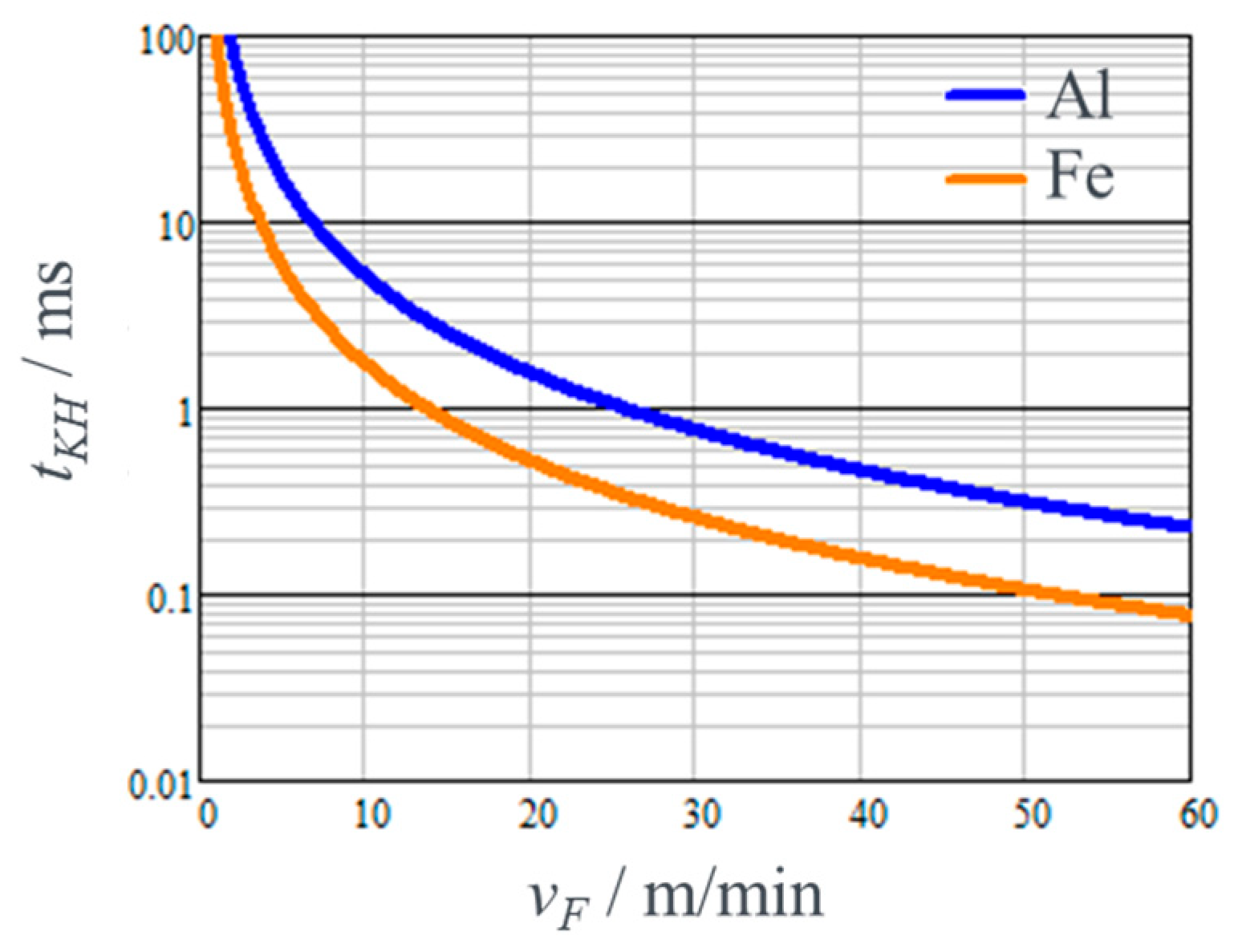
Figure 2.
(a) Main lobe (i.e. “point”) set in the centre of the active area and the accompanying weak diffraction pattern; (b) Point set at an arbitrary position (x,y); (c) Point set at the position (xmax,ymax) where the main lobe and all diffraction lobes have the same maximum intensity.
Figure 2.
(a) Main lobe (i.e. “point”) set in the centre of the active area and the accompanying weak diffraction pattern; (b) Point set at an arbitrary position (x,y); (c) Point set at the position (xmax,ymax) where the main lobe and all diffraction lobes have the same maximum intensity.
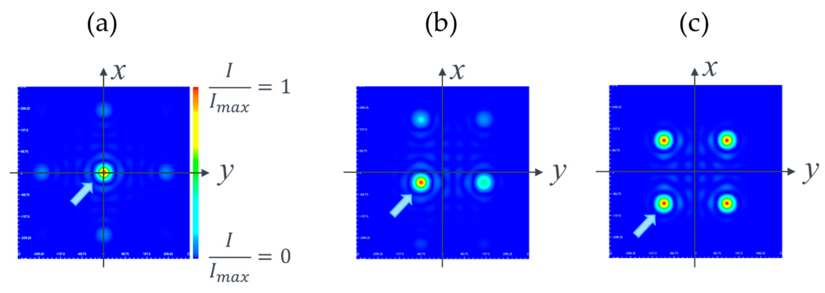
Figure 3.
Examples for shapes created with a sequence of points. NPos is the number of addressed positions used for creating this shape, NSP is the total number of sequentially addressed single points. The spiral and the hourglass shown in (c) and (d), respectively, might be used for example to widen a keyhole. The feed direction is to the right.
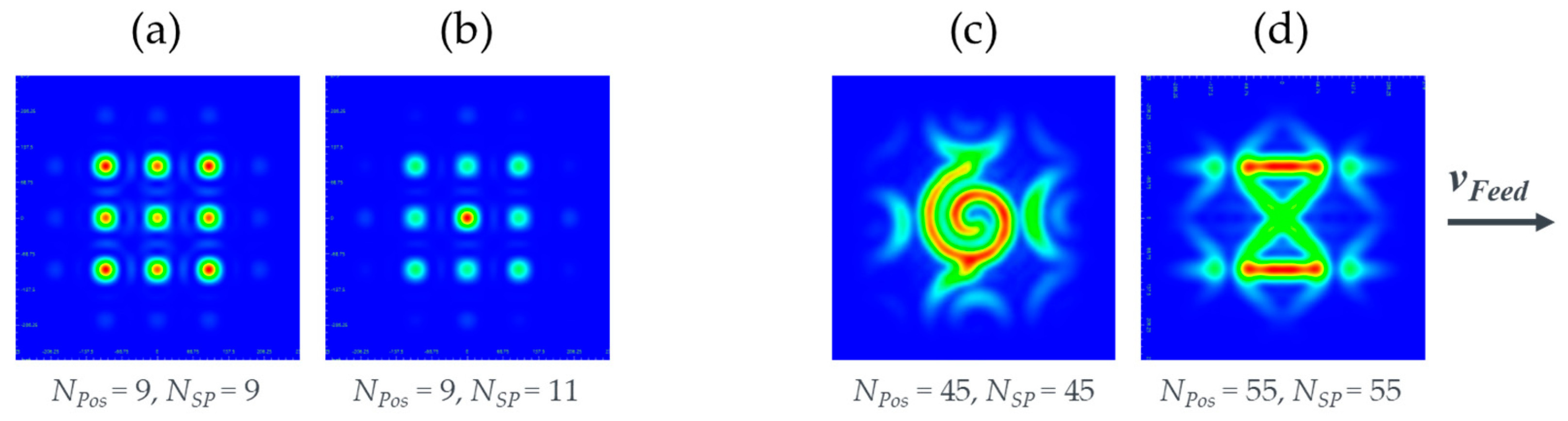
Figure 4.
(a)-(f) 250. µs describing the emergence of a process pore during welding of aluminium with an average laser power of 3.4 kW and a feed rate of 4 m/min. The details are described in the text.
Figure 4.
(a)-(f) 250. µs describing the emergence of a process pore during welding of aluminium with an average laser power of 3.4 kW and a feed rate of 4 m/min. The details are described in the text.
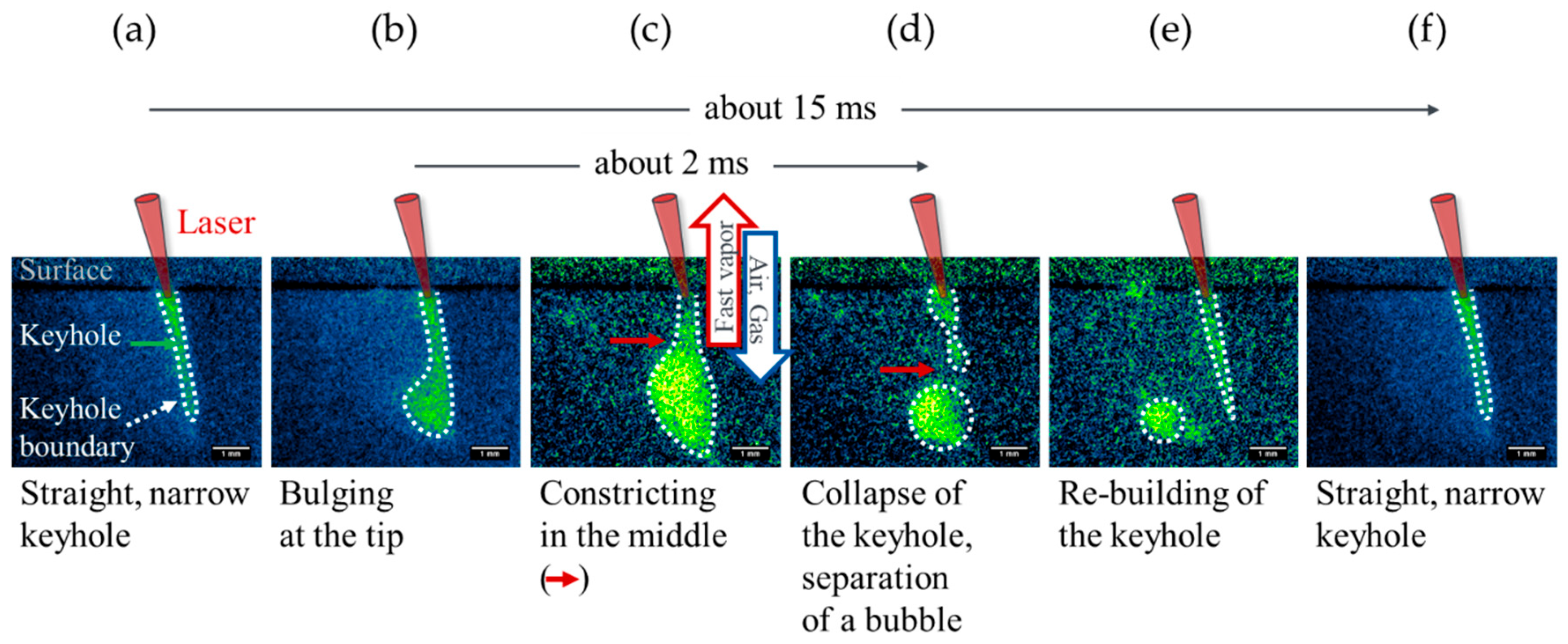
Figure 5.
(a) Spiral beam shape with 45 points used for the experiments. The feed direction is to the right. (b) The process feature ψ = porosity as a function of the shape refresh frequency fSR, which is the the periodic dynamic parameter modification with the frequency in this example. The labels at the top mark the three process regimes identified.
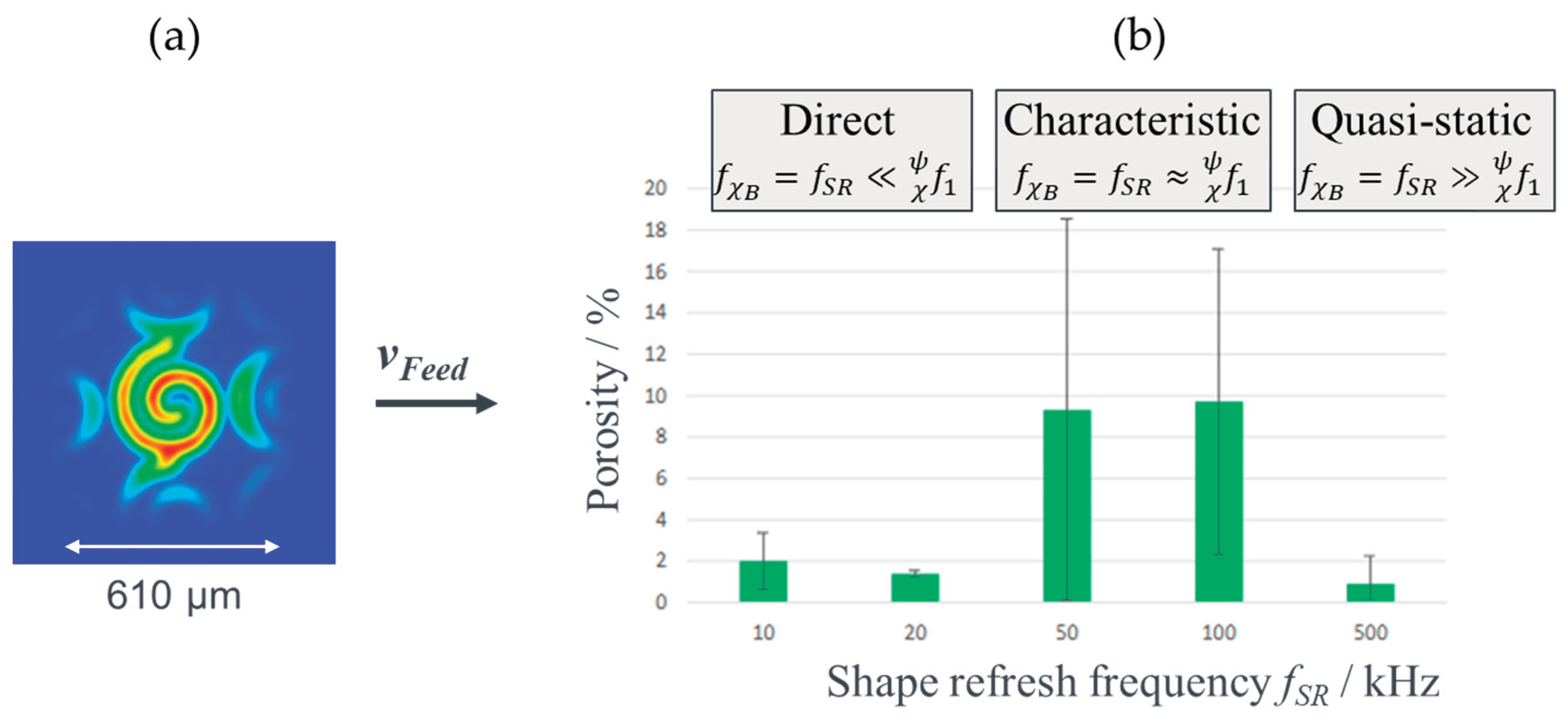
Table 1.
Examples of a few typical process time constants and the respective frequencies for a feed rate of 1 m/s with an average laser power of 10 kW. A thermal diffusion length of ℓD = 0.5 mm and a width of the laser beam on the surface of dW =0.5 mm was taken. is the melting temperature and the vaporization temperature of the respective material.
| Effect | Material | Time (ms) |
Frequency (kHz) |
|---|---|---|---|
| Heat conduction for ℓD = 0.5 mm | Fe | 2.8 | 0.4 |
| Heat conduction ℓD = 0.5 mm | Al | 0.640 | 1.6 |
| Temperature increase TL-TV | Fe | 0.001 | 1000 |
| Temperature increase TL-TV | Al | 0.167 | 6 |
| Sound wave dW = 0.5 mm | Al/Fe | 0.100 | 10 |
| Keyhole collapse | Fe | 1 | 1 |
| Keyhole collapse | Ti | 0.004 | 250 |
Table 2.
Summary of the regimes of dynamic process modifications induce by periodic dynamic beam shaping.
Table 2.
Summary of the regimes of dynamic process modifications induce by periodic dynamic beam shaping.
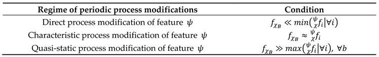
Table 3.
Diameter of the main lobe dML, maximum intensity in the center Imax,0,0, scan width dS, and with of the active area dActiveArea for a few focal lengths of the focusing lens, fL, and a DBL with 12 kW of output power.
Table 3.
Diameter of the main lobe dML, maximum intensity in the center Imax,0,0, scan width dS, and with of the active area dActiveArea for a few focal lengths of the focusing lens, fL, and a DBL with 12 kW of output power.
|
fL (m) |
dML (µm) |
Imax,0,0 (W/cm2) |
dS (µm) |
dActiveArea (µm) |
|---|---|---|---|---|
| 0.75 | 68 | 4.0.108 | 129 | 709 |
| 1.0 | 91 | 2.2.108 | 172 | 945 |
| 1.5 | 136 | 9.9.107 | 258 | 1418 |
| 3.0 | 272 | 2.5.107 | 516 | 2836 |
Table 4.
The example for a “DBL solutions matrix” gives an approach to reducing the formation of process pores and summarizes the possible frequency regimes for the periodic dynamic process modifications.
Table 4.
The example for a “DBL solutions matrix” gives an approach to reducing the formation of process pores and summarizes the possible frequency regimes for the periodic dynamic process modifications.

Disclaimer/Publisher’s Note: The statements, opinions and data contained in all publications are solely those of the individual author(s) and contributor(s) and not of MDPI and/or the editor(s). MDPI and/or the editor(s) disclaim responsibility for any injury to people or property resulting from any ideas, methods, instructions or products referred to in the content. |
© 2026 by the authors. Licensee MDPI, Basel, Switzerland. This article is an open access article distributed under the terms and conditions of the Creative Commons Attribution (CC BY) license (http://creativecommons.org/licenses/by/4.0/).
Copyright: This open access article is published under a Creative Commons CC BY 4.0 license, which permit the free download, distribution, and reuse, provided that the author and preprint are cited in any reuse.


