

Submitted:
10 November 2026
Posted:
13 November 2026
You are already at the latest version
Abstract
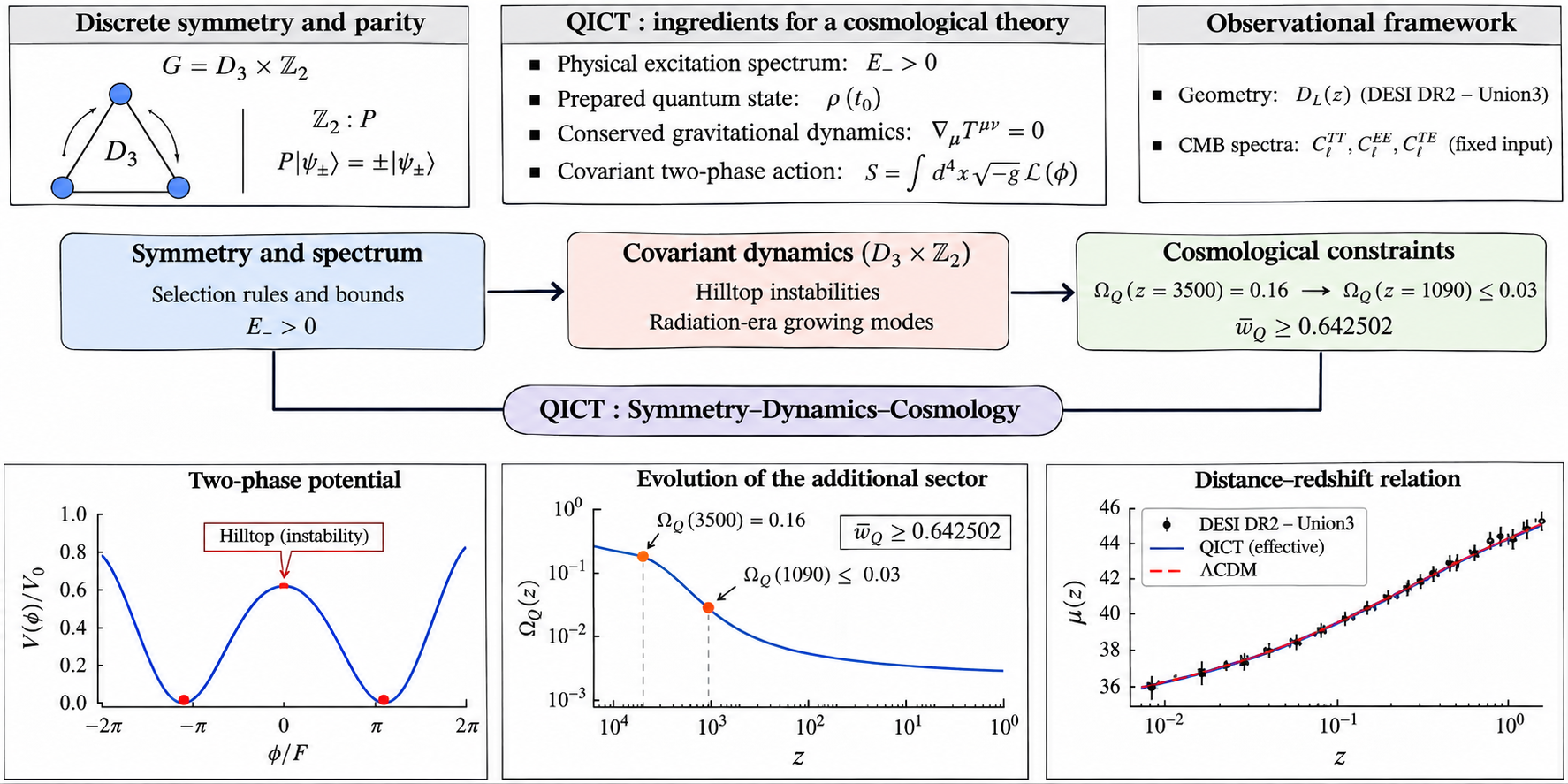
Discrete symmetries offer a mechanism for dark-matter stability, but a cosmological prediction also requires a physical excitation spectrum, a prepared quantum state and conserved gravitational dynamics. We examine these requirements in Quantum Information Copy Time (QICT) through a parity-graded quantum system, a passive receiver response and a covariant \( D_3\times\mathbb Z_2 \) two-phase theory. We derive parity selection rules and positive odd-sector spectral bounds, then show explicitly that the symmetry fixes neither the odd-particle mass nor its occupation. For the covariant action, we calculate the canonical hilltop instabilities and radiation-era growing modes. Conservation of the complete additional sector imposes a quantitative dilution bound: in a specified matter–radiation benchmark, decreasing its fractional density from 0.16 at \( z \) = 3500 to at most 0.03 at \( z \) = 1090 requires \( \overline w_Q \) ≥ 0.642502. We determine the Gaussian one-loop counterterm classes and test a separate effective receiver using correlated DESI DR2–Union3 distances and fixed-input CMB spectra. The geometric fit improvement disappears when a \(\Lambda\)CDM-conditioned matter prior is removed. These results provide reproducible constraints on symmetry-protected excitations, early-universe energy transfer and the interpretation of cosmological response models.
Keywords:
quantum information copy time
; receiver symmetry
; parity-graded quantum dynamics
; spectral reconstruction
; dihedral symmetry
; cosmological energy transfer
; dark matter
; causal susceptibility
; early-universe dynamics
1. Introduction
A discrete symmetry can make the lightest particle carrying a conserved charge stable. It does not, by itself, determine the particle’s mass, its primordial abundance or the way its energy gravitates. These are distinct physical questions. The first concerns the spectrum of excitations above the vacuum; the second depends on the quantum state and the production history; the third requires an energy–momentum tensor that is conserved together with the other cosmological components. A dark-sector construction becomes predictive only when these ingredients are supplied by compatible dynamics. This distinction is especially important when a collective response is used to modify the expansion history while a separate symmetry protects a dark-matter candidate.
Quantum Information Copy Time (QICT) offers a mathematical setting in which these requirements can be examined separately and precisely. We study a parity-graded quantum system, a spatial record-transport model with passive receiver response, and a covariant two-phase action invariant under . Each is specified by its own Hamiltonian, constitutive map or field-theoretic action. They are subject to common symmetry and conservation tests, but their generators and physical scales are not identified without calculation. In particular, a pole in a macroscopic susceptibility is not automatically the mass pole of a parity-odd particle. Distinguishing the two prevents a homogeneous cosmological fit from being mistaken for microscopic mass determination.
The first result concerns the operator meaning of dark parity. An exact grading yields selection rules for even observables and protects a lightest odd asymptotic state when such a state exists. Positivity of the odd-sector spectral measure provides a complementary condition on its Euclidean correlator and pole weight. These statements require neither a particular particle mass nor a choice of initial occupation. We make their logical limits explicit through a parity-invariant scalar completion with continuously variable positive mass and through even quantum states with different odd-mode populations. Open-system covariance is treated separately from local conservation of the subsystem charge, since an environment can carry the conserved total parity [16,17].
The second question is whether a receiver response can support a consistent cosmological source. Spatial record transport defines an operational registration scale; a specified passive constitutive relation then yields positive homogeneous Friedmann branches and bounds on the acoustic horizon. The width of a positive mixture of relaxation times is constrained, whereas a coherent resonance belongs to a different response class. These are statements about a declared effective density map. They do not establish that the finite-charge phase theory generates that map. The necessary matching would be a retarded response calculation with fixed source normalization and a consistent gravitational perturbation sector.
The third question concerns the early-universe evolution of the covariant action. We give its phase metric, potential and independent parameters in the main text, then calculate the two canonical unstable directions at the symmetric hilltop and their regular radiation-era growing modes. The resulting linear instability describes sensitivity to initial displacement; it is not a mechanism that selects that displacement. A separate and particularly restrictive constraint follows from exact conservation of the full additional energy. Conversion of coherent phase energy into stable odd quanta changes the partition between components, but does not eliminate their total gravitational contribution. For a specified positive extra component, this fact yields an integrated equation-of-state threshold and an earlier-epoch bound that any proposed rapid transition must satisfy.
We test the effective cosmological response with two deliberately distinct numerical procedures. A compressed geometric analysis uses the released correlated DESI DR2 baryon-acoustic-oscillation measurements and Union3 supernova data, together with an explicitly identified acoustic-angle summary. A separate fixed-input CAMB calculation follows the multipole response of a prescribed effective fluid. The compressed likelihood is useful for investigating parameter identifiability and sensitivity to external priors, but it is not a native Planck–ACT–DESI likelihood for the interacting finite-charge theory. In particular, the apparent preference of the one-pole receiver disappears without a matter-density prior conditioned on the reference CDM model [9,24,25].
The purpose of this article is to turn symmetry protection, spectral identification and cosmological energy transfer into independently testable statements within QICT. The main text contains the defining actions, theorems, quantitative bounds and observational diagnostics. The accompanying Technical Supplement provides the extended proofs, quantum-state and renormalization analyses, initial-value studies, covariance matrices and executable tests. Keeping these constructions separate where no microscopic matching has been established is essential to the physical interpretation of the results.
2. Materials and Methods: Effective Model and Test Design
Three mathematical constructions are kept distinct throughout the analysis. The operator sector assumes a self-adjoint grading commuting with the physical evolution and uses positive-energy spectral theory. The open-system sector models registration of an encoded record with an explicitly normalized spatial diffusion process and a phenomenological map from its transport scale to a gravitational density. The covariant finite-charge sector specifies a field action, its initial data and its energy–momentum tensor. Agreement of a selection rule across these constructions is a consistency check, not a proof that their microscopic degrees of freedom coincide. We use natural units unless SI conversions are displayed, with .
The homogeneous one-pole receiver is the model entering the numerical distance analysis. The constant-plus-transport and logistic-response branches are independent effective comparators; their input dictionary appears in Online Resource 2. We use 13 correlated DESI DR2 BAO observables and the 22-dimensional Union3 supernova compression, retaining the supplied within-survey covariance matrices. The supernova absolute-magnitude intercept is eliminated analytically by generalized least squares. An acoustic-angle summary and, in a separate variant, a CDM-conditioned Gaussian prior on the physical matter density provide explicitly identified screening constraints. Baryon loading and the recombination and drag redshifts are fixed in these compressed calculations. None of these inputs is substituted for a primary-CMB multipole likelihood of the coupled field theory.
Analytic identities, independent numerical integrations and consistency checks are retained with their source files. The archive includes finite-dimensional GKSL and scale-cancellation tests in Supplementary Section ??, nonlinear phase-space integrations, covariance diagnostics, regulator studies and a fixed-input CAMB fluid benchmark. The reported numerical environment used Python 3.13.5, NumPy 2.3.5, SciPy 1.17.0 and Matplotlib 3.10.8; portable dependencies and execution instructions accompany the code. Each computational result is associated with the action, state, data compression and approximation actually used to obtain it.
2.0.0.1. New results and proofs.
The established ingredients of the analysis are parity selection, completely positive quantum transport and canonical scalar reconstruction. Results specific to the stated constructions include an explicit parity-safe odd-particle completion, a positive odd-sector spectral criterion, a bounded-perturbation gap estimate, existence and uniqueness of the passive Friedmann branches, acoustic-contraction and spectral-width inequalities, canonical longitudinal and transverse hilltop curvatures, and exact conservation thresholds for an early additional component. We also test whether the finite-charge action fixes a mass or quantum occupation, derive the Gaussian odd-sector counterterm classes, and reoptimize the compressed distance screen against its nested CDM branch. Proofs and numerical checks are identified separately; a conditional effective-model result is not promoted to a universal statement about an unspecified microscopic QICT generator.
3. Scope of the Mathematical and Effective Realizations
The constructions developed in this article share symmetry constraints but differ in their dynamical inputs. An operator result can be applied to a particular cosmological action only after the relevant representation, physical source, and scale are specified. Table 1 records those domains of inference and makes the numerical comparisons unambiguous.
Covariant finite-charge realization and its independent parameters
For the early-universe phase analysis we fix a separate, explicit effective action. With , and integer , define
The choice of three oriented phase differences makes invariant under the dihedral action specified in Supplementary Section ??. The independent odd grading acts as and leaves q unchanged. The covariant action, with signature , is
Here and . These are independent effective parameters unless a separate microscopic matching calculation constrains them. At the phase energy and pressure are
The quadratic odd fluctuation has in a homogeneous background, before loop corrections. The real scalar s in Eq. (13) below is a simpler parity-invariant comparator, not an identified field redefinition of . Likewise, neither the passive receiver map nor its crossover scale follows from Eq. (3) without an independent calculation of the corresponding response function. The action, conservation law and parameter status are part of the main article so that its early-universe conclusions do not rely on an unstated dynamical model.
Proposition 1
(Parity does not identify the rest mass). The symmetry and the specified finite-charge potential do not determine a unique odd-particle rest mass. In the invariant subfamily , every gives an allowed free odd scalar with an isolated positive-residue pole at on the translation-invariant vacuum.
Proof.
Neither nor the grading depends on the coefficient of . The kinetic term remains positive and invariant when that coefficient is replaced by any other positive value. The free two-point function then has a simple pole at the corresponding mass, with the same even-sector action and selection rules. Distinct positive therefore satisfy all stated symmetry hypotheses. The interacting pole requires an additional renormalization condition and microscopic matching. □
Logical matching conditions
The parity-graded system, diffusive receiver and finite-charge action have independently defined parameters. A single microscopic model connecting them would need to exhibit: (i) a representation of the odd grading and its spectral pole in the covariant particle field; (ii) a derivation of and of the gravitational response map from one calibrated generator; (iii) a physical state and collision or quantum-kinetic evolution fixing the renormalized stress tensor; and (iv) perturbations derived from that same stress tensor and evaluated with the relevant observational likelihoods. None of the theorems below requires an unproved identification across these steps. In particular, the homogeneous one-pole distance screen is not used as an observational test of Eq. (3).
4. A Discrete Dark-Sector Symmetry and Its Physical Selection Rules
Consider a physical Hilbert space and a self-adjoint involution with both eigenvalues represented,
This grading may be global or descend from a discrete gauge symmetry. Its specific ultraviolet origin does not enter the selection results below. The central assumption is that commutes with the exact positive-energy generator and with the physical scattering evolution. The lightest massive odd asymptotic state is a candidate for stable dark matter when all lighter visible species are even.
Theorem 1
(Parity protection of the lightest odd state). Let be self-adjoint, bounded below and parity preserving. Suppose an odd one-particle state of mass is the lightest allowed asymptotic state carrying odd parity, and that its on-shell energy-momentum is conserved. Then a decay of that particle entirely into lighter even particles is forbidden. A decay into a state with odd total parity is kinematically forbidden when every such final state has invariant mass at least and the decay products possess strictly positive relative kinetic energy.
Proof.
The scattering operator preserves the parity eigenvalue. Hence a nonzero amplitude from an odd initial state requires an odd final state, excluding a final state made entirely of even particles. Any remaining final state contains odd charge. The assumed lightest-mass ordering and on-shell energy-momentum conservation then exclude a kinematically lighter multiparticle channel. □
Proposition 2
(Parity selection of even observables). If and , then
If an even vacuum exists and , then .
Proof.
Conjugation by leaves invariant and changes the mixed-parity matrix element by a minus sign. The analogous calculation with the odd observable changes the vacuum expectation by a minus sign. Both matrix elements vanish. □
In particular, a parity-even stress tensor has vanishing vacuum-to-single-odd matrix elements. Cosmological gravitational responses can contain even composites, dark-particle populations and pairs of odd excitations. A parity grading protects particle stability without equating the collective response to an individual odd particle.
Theorem 2
(Positive odd-sector spectral measure). Let have an even ground state of energy , with odd-sector spectral gap . For a bounded parity-odd operator and , define
Then is positive, supported on , and its Euclidean two-point function satisfies
An isolated spectral atom at with positive weight contributes and identifies a positive source residue.
Proof.
The odd operator maps the even ground state into . Restricting the spectral theorem to that subspace proves positivity and the support statement. Functional calculus gives the Laplace representation and its exponential upper bound. Isolating the atomic part yields the final assertion. □
The conditions in Theorems 1 and 2 form the symmetry contract for a stable dark species. The particle mass and cosmological abundance additionally depend on a specified Lagrangian or microscopic spectrum and its interactions.
Proposition 3
(Energy-gap stability under parity-preserving perturbations). Let and be the infima of the even and odd spectra of a parity-preserving Hamiltonian and . If a bounded, self-adjoint perturbation K preserves parity and , then
Proof.
The variational principle gives in each parity sector. Subtracting the resulting inequalities yields the claim. □
5. Reduced-channel Covariance and the Dark-Charge Bookkeeping
A reduced channel can preserve the grading symmetry while exchanging the corresponding charge with an environment. Let be involutions, let , and set
Theorem 3
(Covariance versus local charge conservation). If , then
If also , then .
Proof.
Conjugate the system–environment input by , commute this product through and use the invariance of the partial trace. Under the second commutation relation, move through the evolution inside the Heisenberg expectation value. □
For an explicit separation, take two qubits with , an even environment , and . Total parity is conserved, yet an odd subsystem input becomes even while the environment acquires the odd charge. The example is an exact reduced-channel illustration; it is independent of a particular microscopic QICT gate architecture.
6. An Explicit Parity-Invariant Dark-Matter Completion
The symmetry theorem admits a minimal low-energy field-theoretic completion, separate from the microscopic transfer problem. Let s be a real dark scalar odd under and let be an even scalar representing the collective receiver response. On a Lorentzian spacetime with metric signature , consider
where , , , and is even under . The action is invariant under
The mass of a small odd fluctuation in a prescribed even background is
The parity-symmetric background is a local minimum of the s-potential. Its elementary odd fluctuation has no tadpole and no parity-allowed vertex with a single external s field. A positive physical mass in the interacting theory additionally requires the renormalized two-point function to have a positive isolated pole residue.
Proposition 4
(Compatibility of the odd particle and even cosmological source). For the action in Eq. (13), the stress tensor is parity even, and all linear matrix elements from an even vacuum to a single odd excitation vanish. The even scalar may contribute a nonzero homogeneous stress tensor without selecting a vacuum expectation for the odd scalar.
Proof.
Every term in the action contains the odd field with even total power. Its metric variation therefore preserves parity. Equation (6) proves the vanishing matrix element. The equation of motion for s is homogeneous at because the potential derivative with respect to s vanishes there, while the equation for contains its independent potential derivative . □
A population of stable odd quanta can source an effective cold-dark-matter fluid while maintaining . For a collisionless nonrelativistic ensemble with number density and negligible production and annihilation after decoupling,
For constant mass, and , recovering the background cold-dark-matter scaling. If varies adiabatically with the receiver field, the background matter-energy equation becomes
Their sum is exactly conserved. Equation (17) makes explicit the difference between an exchange of energy induced by a changing dark-particle mass and a pure momentum-exchange model, which preserves the homogeneous density of each component separately.
The one-pole receiver background has a canonical-scalar representation along its homogeneous trajectory. The action in Eq. (13) establishes a parity-respecting low-energy field content; a finite introduces a field-dependent odd-particle mass and the background energy exchange in Eq. (17). The separately conserved one-pole reconstruction is therefore recovered on the or dynamically negligible-exchange branch. An interacting realization instead solves the coupled scalar and odd-matter equations. The physical masses and abundances are inputs to the corresponding spectral and thermal calculations.
6.1. Relic Abundance and Particle Stability as Distinct Tests
A thermally produced odd species would require an interaction rate and an entropy history. Its comoving abundance obeys, in the conventional freeze-out approximation,
when entropy is conserved and is approximately constant across decoupling. The exact symmetry explains stability, whereas Eq. (18) fixes the relic abundance only after specifying the interaction rate and expansion history. This is a useful separation for a phenomenological dark-sector model: stable particles need not have the observed cosmological number density without an appropriate production history.
Proposition 5
(State-dependent odd abundance at fixed action). The action and parity can be held fixed while the particle number of an even quantum state varies. For two opposite-momentum odd modes , the normalized states
are parity even, but their mean occupation in either mode is . Hence parity alone cannot specify the initial dark-particle density.
Proof.
Each summand contains odd quanta and therefore has parity . The geometric series normalizes the state. Differentiation of its generating series gives , which varies continuously while the Hamiltonian and parity operator are unchanged. □
For a cosmological continuum, a smooth Bogoliubov coefficient with compact support in comoving momentum produces the corresponding ultraviolet-regular family, as derived in Supplementary Section ??. This is a state-identifiability obstruction, not a proposal for a preferred primordial state.
7. A Conservation Criterion for Parity-Preserving Dark Interactions
The effective action permits a parity-even interaction between the odd particle and the collective scalar. This coupling retains the exact charge while exchanging energy between the two cosmological components. The resulting conservation law fixes when the separately conserved receiver branch used in the geometric analysis is an exact limit of the interacting model.
Proposition 6
(Mass-varying dark matter and the receiver exchange). Assume a nonrelativistic ensemble of odd quanta with conserved comoving number, , and a positive adiabatic mass
Its energy transfer to the dark-matter component is
On every open time interval on which and , a strictly positive produces . The separately conserved one-pole receiver reconstruction is therefore the limit, while nonzero exchange defines a coupled-background realization.
Proof.
Differentiating and using number conservation yields . The derivative gives the first identity. Total conservation gives the second. Every factor in the remaining assertion has the stated sign or nonvanishing condition. □
This criterion separates two coherent phenomenological prescriptions. A decoupled receiver () supports the homogeneous one-pole analysis and canonical scalar perturbations employed in the geometric screen. An interacting dark ensemble () requires the coupled scalar, particle and Einstein equations with their common initial conditions. Parity conservation remains exact in both regimes and by itself fixes neither the relic density nor the coupling strength.
8. Phase Covariance and a Reduced-State Source
Consider a reduced density operator obtained from a bipartite state by . A time-local, completely positive divisible evolution has a generator of Gorini–Kossakowski–Sudarshan–Lindblad form
under the usual operator-domain assumptions [16]. The non-negative rates in Eq. (21) ensure a completely positive intermediate propagator; more general non-Markovian time-local descriptions need not have non-negative rates [17,18].
Let a be an annihilation-like mode and let denote the physical phase reference. Define
The source is real for real . Under the simultaneous rephasing and , is unchanged. Thus the phase entering a real homogeneous observable is meaningful only relative to a phase reference; an isolated complex phase is not an additional gravitational degree of freedom.
Proposition 7
(Quadrature bound). For any reduced state with finite occupation ,
Consequently, for all such states if .
Proof.
The Cauchy–Schwarz inequality for the positive functional gives . Equation (23) follows by taking the real part. The lower bound on the total density is immediate. □
Theorem 4
(Parity-compatible receiver source). Let be a conserved self-adjoint involution, and let the homogeneous reduced state satisfy . The phase reference θ is parity even. Decompose any mode into -even and -odd components, . Then
A nonzero homogeneous linear source in a parity-symmetric state therefore belongs to the even receiver channel. Odd-field contributions to the stress tensor arise from parity-even composites and populations.
Proof.
Cyclicity of the trace and parity invariance imply
The odd expectation vanishes. Substitution into the quadrature identity gives Eq. (24). The stress tensor is parity even by the invariance of the action under metric variation. □
The theorem also distinguishes a coherent odd condensate, which would select a parity-breaking state, from an even statistical population of stable odd particles. A Hermitian source is real while its positivity depends on the state. Identifying that expectation with the gravitational collapse-bound density requires a further constitutive coupling equation; this manuscript specifies the positive cosmological density separately.
9. Local Record Transport and the Copy-Time Scale
An unknown quantum state cannot be cloned deterministically [19]. Here copy time refers to the propagation and registration of a distinguishable, encoded record, not the duplication of an arbitrary unknown state. Consider the one-excitation tight-binding chain
Its master equation is
Let and . The exact population continuity equation is
The sign and relative orientation of the neighboring currents are fixed by . On length scales large compared with a and in the dephasing-dominated regime, eliminating rapidly relaxing coherences gives
Here the error notation refers to the controlled long-wavelength, small- expansion rather than a uniform-in-time bound on all density matrices. The continuum diffusion coefficient is
The exact continuity equation and the leading approximation are derived independently in Online Resource: Cosmology Methods.
For an isotropic diffusion process in d dimensions, the mean-square displacement satisfies . A fixed root-mean-square registration threshold L therefore defines
For other explicitly calibrated thresholds, incorporates the corresponding dimensionless factor. The symbol is deliberately distinct from the entropic clock : the latter is a state-dependent entropy-production time and is not identical to a transport time for general stationary states.
10. Gravitational Admissibility and the Effective Response
The ultraviolet–infrared restriction of Cohen, Kaplan, and Nelson motivates a gravitational energy scale proportional to [20]. We express its finite-coefficient implementation as the inequality
Writing introduces a saturation fraction . It follows exactly that
Thus an H-linear contribution arises when is approximately constant. The inequality alone does not determine f, and a time-dependent changes the background response.
We examine a minimal constant-plus-transport class,
with , , and . Within the cutoff construction, this is equivalent to prescribing
Equation (34) is the constitutive input. In particular, its term generates a constant energy-density component; it is not supplied by a quantum speed limit without an additional dynamical calculation. With a constant , the cutoff condition becomes the directly testable bound
In physical units, the dimensionless factor is . For the monotone physical solution on derived below, , so the simple sufficient condition
ensures gravitational admissibility throughout that redshift domain. This is a bound on an effective medium parameter, not a microscopic prediction of the diffusion constant.
11. Transition Kinetics and Redshift Dependence
A local algebraic interpolation is
It is smooth and increasing with z, and tends toward unity at high redshift. A kinetic interpretation is possible, but the cosmic-time equation and the redshift interpolation have different global forms. For an occupancy obeying
the exact redshift evolution is
Its integral representation involves . Matching derivatives at the transition to Eq. (37) gives
which is an exact local slope identity, not an exact identification of the functions over all redshifts. The fit class Eq. (37) admits an explicit Friedmann solution, while Eq. (39) gives a coupled first-order background system. Both are internally specified and need not be conflated. For the kinetic branch, determines , where is obtained from the coupled kinetic–Friedmann boundary-value problem. The existence, uniqueness and admissibility of that boundary-value solution are verified for each specified parameter domain; the algebraic branch result alone does not establish global shooting uniqueness.
12. Exact Homogeneous Dynamics
For a spatially flat FLRW geometry with separately conserved matter and radiation, the Friedmann equation of the effective model reads
For the fitted switch, prescribing a matter–dark-sector equality redshift also permits an explicit parameter dictionary. With , and , one finds
with subsequently fixed by normalization. This is a reparametrization conditional on the supplied and the positivity of the resulting density fractions; the proof appears in Online Resource: Cosmology Methods.
Normalization fixes
Set .
Theorem 5
(Positive branch, monotonicity and non-phantom equation of state). Suppose , , , and with and . Then Eq. (41) has exactly one positive solution,
It is continuously differentiable and obeys
If is separately conserved, its effective equation of state satisfies . The inequality is strict whenever and .
Proof.
The quadratic has roots with negative product . Its positive root is Eq. (44); the denominator of Eq. (45) equals the strictly positive discriminant square root. As and , . Separate conservation gives , and Eq. (33) implies
Every factor in the correction is non-negative for and the denominator is positive. □
Corollary 1
(Present acceleration criterion). Under the hypotheses of the theorem and , present acceleration is equivalent to
Proof.
At , . The denominator is positive. The inequality is precisely Eq. (47). □
If at high redshift, the transport term grows as while matter and radiation grow as . In radiation domination,
and, in a matter-dominated range, . The constant component is more strongly suppressed. These are homogeneous-background statements; acoustic-scale perturbations require independent calculation.
13. A Single-Scale Receiver Response and the Acoustic Horizon
The H-linear term is negligible relative to the critical density at recombination: for , . A change of the microscopic receiver saturation law is therefore required for an appreciable acoustic response. We consider a bounded one-scale constitutive law,
The constants are written in units ; when SI units are used, D in Eq. (50) is replaced by . The scale is the crossover of the effective receiver response, a phenomenological collective crossover scale.
Theorem 6
(Unique one-scale homogeneous branch). Let with , , and . The equation
has one and only one positive solution for every . Its fractional receiver density obeys , with the maximum attained at . The branch is differentiable and nondecreasing with redshift.
Proof.
Put and . Then
The inequalities and imply for and . Also and . Thus the equation has a unique positive root. Differentiating shows . Finally , with equality only at . □
Corollary 2
(Unified positive branch with late transport). Let , , with , , and with . Write . If
then the combined receiver equation
has exactly one positive solution for every , and this solution is nondecreasing with z. The exact normalization is .
Proof.
Every positive root satisfies , since . The derivative of the left side with respect to E is bounded below by , which is positive throughout the possible root domain by Eq. (53). The left side minus is negative at and tends to , so its root is unique. Implicit differentiation yields . □
Normalization requires . The isolated one-pole sector has the separately conserved homogeneous equation of state,
At , ; at , . Consequently its fractional density is suppressed at both ends of the expansion history. The one-scale law is a conditional response of the QICT effective theory; a microscopic spectral calculation must determine , D and .
Proposition 8
(Reciprocal spectral envelope and logarithmic sum rule). For , the one-pole fractional density satisfies
Hence the response height, reciprocal shape and integrated logarithmic weight are fixed by the same amplitude λ.
Proof.
Writing gives . The reciprocal relation follows from , and proves the integral identity. □
Theorem 7
(Acoustic fraction bound). Let for , and hold the photon–baryon sound speed and drag epoch fixed. If , then
In particular, a target ratio requires .
Proof.
Substitute . The ratio is the weighted average of with positive weight . Bounding the integrand pointwise proves the result. □
13.1. Quantitative Test and Observational Distinction
The updated numerical calculation uses , , , km , fixed , and . The baryon–photon sound speed is , evaluated using . Table 2 gives reproducible calculations. The original late transport term is set to zero for this isolated acoustic benchmark. Restoring produces a unique combined background under Eq. (53); recalibrating the same acoustic proxy gives , compared with in the isolated branch. The late contribution shifts the acoustic integral by less than one part in a million in this example.
Figure 1.
Receiver fraction for a single crossover scale. Both asymptotic regimes are suppressed, and the peak position is fixed by . The profiles are homogeneous toy-model solutions, not perturbation fits.
Figure 1.
Receiver fraction for a single crossover scale. Both asymptotic regimes are suppressed, and the peak position is fixed by . The profiles are homogeneous toy-model solutions, not perturbation fits.
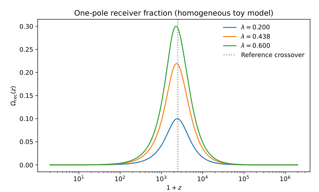
For illustration, the numerical ratio requires by Eq. (57); the chosen one-pole shape attains this proxy at . In a different analysis, Poulin et al. found and km in a profile-likelihood study of a distinct early-dark-energy model [10]. Its constraints do not transfer numerically to Eq. (50), but they identify the CMB level at which the one-pole benchmark must be tested. A multiprobe study of a distinct early-dark-energy family reports 95% constraints as restrictive as in its Planck-based combination [11]. Newer ruler-free reconstructions also give a broader local-expansion range, km [21].
The symmetry of the cosmological background provides a complementary route to analyzing the expansion scale [22]. The acoustic ratio alone is not an inferred : CMB peaks determine both an angular scale and phase information, while BAO and calibrated supernovae constrain absolute and relative distances. Joint data can therefore change the best-fit value of as well as itself. In particular, independent analyses have found geometric tensions between BAO and supernova distance shapes that survive a uniform rescaling of the ruler [23]. A valid receiver-sector resolution must predict the full temperature, polarization, lensing and matter spectra, rather than assign through the proxy ratio.
Proposition 9
(Time reparametrization does not change the measured expansion). For a spatially flat FLRW metric , any monotone change of time coordinate with lapse leaves the physical expansion scalar invariant. A copy-clock reparametrization alone therefore cannot change a locally measured Hubble parameter.
Proof.
In the T coordinate the metric is , with . Consequently,
independently of the time coordinate. □
The requisite microscopic statement is thus a physical constitutive response in the stress tensor, rather than a relabeling of time. If a spectral calculation gives a different dependence , the acoustic theorem and the test program remain applicable.
14. Spectral Passivity, Response Width and Collective Resonance
The acoustic-fraction theorem bounds the amplitude of early energy, while its temporal support is governed by the spectral structure. Positive mixtures of relaxation channels obey a universal logarithmic-width inequality. Collective oscillatory modes offer a distinct form of spectral localization within the same homogeneous framework.
Theorem 8
(Logarithmic-width bound for positive relaxation spectra). Let μ be a finite positive measure on , and define for
Then
Proof.
For each positive , the kernel has logarithmic derivative , which lies in . Differentiation under the finite positive integral is justified locally by the bounded derivative . The derivative of is a positive weighted average of the individual logarithmic derivatives. Integration between and gives the two-sided ratio bound. □
This inequality is specific to positive mixtures of relaxational kernels. It quantitatively couples receiver energy at neighboring expansion rates, giving the acoustic calculation a spectral test of how narrowly an early contribution can be localized. Oscillatory collective modes define the complementary response class.
A causal second-order collective susceptibility offers a minimal such structure,
Its absorptive part is nonnegative for positive frequency in the convention. Identifying the cosmological characteristic frequency with defines the effective fractional receiver density
The identification is a constitutive prescription: Eq. (60) specifies the causal response, while Eq. (61) specifies how its dissipative channel enters the cosmological stress tensor.
Theorem 9
(Simple sufficient condition for a unique resonant Friedmann branch). Let and . If
then the equation has exactly one positive solution for every . For a monotone reference expansion, the solution is monotone. The associated receiver density increases with H along this branch.
Proof.
Put , and . Then and
For this derivative is nonpositive, and . For and , , so . Hence
The function vanishes at , tends to infinity as , and is strictly increasing, proving existence and uniqueness. Finally, is proportional to ; its logarithmic derivative with respect to t is . □
The sufficient condition includes the underdamped interval . Separate conservation and then give from the monotonic receiver energy.
Figure 2.
Receiver energy fraction along two self-consistent homogeneous solutions with similar contraction of the drag-epoch sound horizon. The resonance shifts energy from equality toward last scattering; observational viability depends on the full photon, neutrino and gravitational perturbations.
Figure 2.
Receiver energy fraction along two self-consistent homogeneous solutions with similar contraction of the drag-epoch sound horizon. The resonance shifts energy from equality toward last scattering; observational viability depends on the full photon, neutrino and gravitational perturbations.
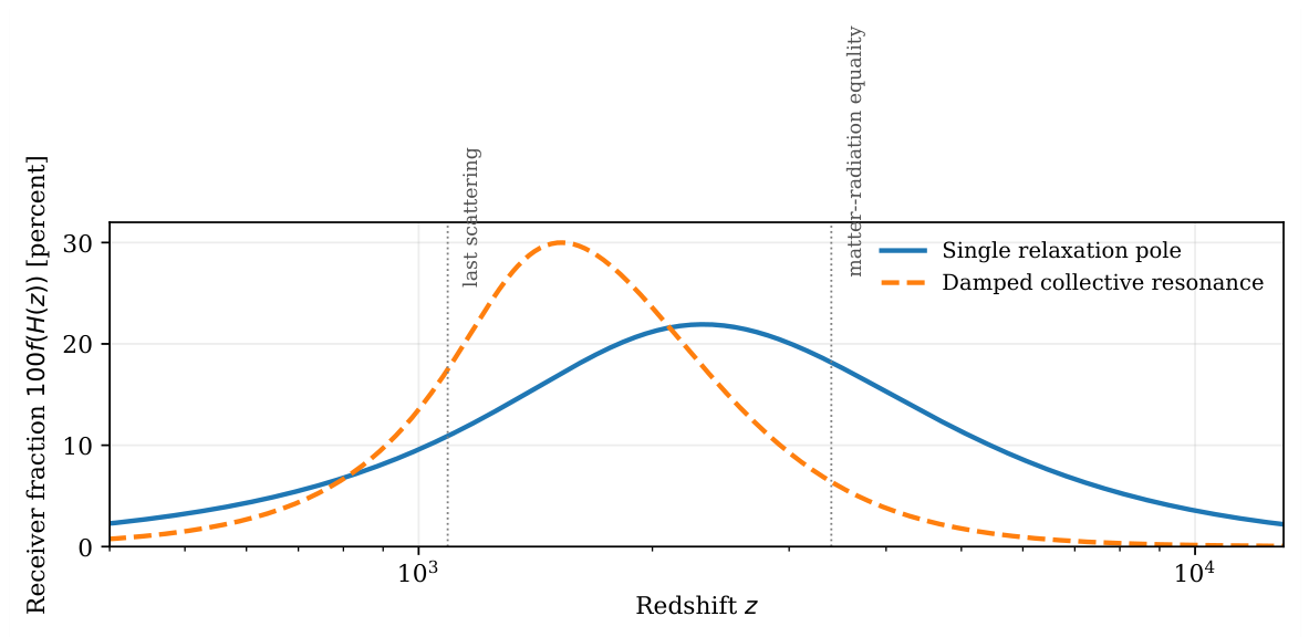
The numerical comparison fixes , the reference sound speed and the drag redshift. Although the two branches give comparable acoustic contraction, their energy fractions differ markedly around equality and last scattering. These differences enter gravitational-potential evolution, peak heights and diffusion damping. Online Resource 3 supplies the benchmark values and branch checks.
For comparison, preserving equality by adding conventional free-streaming radiation to a hypothetical shift of from to requires at fixed . The 2026 combined BBN–CMB–BAO analysis of Goldstein and Hill reports a 95% upper bound within its free-streaming-radiation assumptions [14]. The receiver resonance is a distinct hypothesis and its perturbative signatures require direct comparison with the same precision data.
A recent microscopic symmetry-breaking model with dark-radiation–matter decoupling illustrates the importance of simultaneously specifying dark-sector excitations and their interactions [12]. The receiver construction adds a complementary spectral condition: Eqs. (60)–(61) determine a causal benchmark whose amplitude A, crossover frequency and damping rate are measurable effective parameters. Their microscopic values would be fixed by an independently calculated reduced-state response.
15. Spectral Admissibility and Cosmological Bounds
The single-pole response belongs to a larger positive-relaxation class. It is useful to isolate the consequences shared by every nonnegative superposition of its spectral kernels, independently of the number or distribution of relaxation rates. Throughout this section the response fraction refers to the actual fractional energy density, , and denotes the physical Hubble expansion rate. The reference source includes matter, radiation and any separately conserved constant component; it is held fixed in the following mathematical comparison.
Theorem 10
(Friedmann uniqueness for positive relaxation spectra). Let μ be a finite nonzero positive Borel measure on , and define
Then the equation
has exactly one positive solution for every . If B is differentiable and nondecreasing for , this solution is differentiable and nondecreasing. If the receiver stress tensor is separately conserved, its equation of state satisfies
In particular, under the stated assumptions.
Proof.
For each , obeys . The integral and its derivative are therefore locally well defined, and the positivity of gives
For every fixed , as and as . Since , dominated convergence yields at both ends. Hence as and as . Strict monotonicity proves the stated existence and uniqueness, while proves the cosmological monotonicity. Finally, implies
Separate conservation and establish Eq. (65). □
The bound is sufficient rather than necessary. Its role is to control the combined derivative of the Friedmann term for an entire positive spectral class. The theorem assumes an ordinary effective stress tensor with separate receiver conservation. If the receiver exchanges energy with the odd-particle sector, the exchange source appears explicitly in the continuity equation and the equation-of-state bracket is replaced by its sourced counterpart. A positive spectral weight can arise from a passive dissipative response, but the identification of this weight with a gravitational fractional density remains an independent constitutive requirement.
Corollary 3
(Non-phantom sector and a high-redshift spectral floor). Under the hypotheses of Theorem 10, let be two expansion rates. Then
For a separately conserved receiver on a monotone expansion history, the same spectral class has . Hence a positive superposition of ordinary relaxation kernels has a quantitative lower floor at neighboring epochs and a definite non-phantom equation-of-state signature.
Proof.
Integrate between and . The equation-of-state inequality follows from Theorem 10. □
The two-epoch inequality constrains the redistribution of receiver energy between matter–radiation equality and last scattering. A damped collective resonance lies outside the positive-relaxation mixture and can exhibit a different profile; its CMB signature is determined by the corresponding perturbations.
Theorem 11
(Acoustic weighted-moment bracket). Fix the sound speed , drag redshift , and reference background . For a nonnegative fractional source with , define the acoustic probability weight
If , then
The upper bound is attained by a constant fractional source on the acoustic integration interval; the lower bound is approached by sources concentrated near the endpoints .
Proof.
By definition, . Since for , the lower inequality follows. Concavity of the square-root gives . Squaring the nonnegative sides yields . □
For a nominal acoustic contraction, Eq. (68) requires . This is a constraint on the sound-horizon-weighted average of the extra energy fraction, complementary to the peak requirement obtained from the pointwise envelope. These statements hold at fixed and ; a complete recombination treatment updates both functions self-consistently. A resonant source is subject to the same moment bracket even when it falls outside the positive-relaxation mixture of Theorem 10. The difference between these response classes is expressed by their support in redshift and by their perturbation dynamics, not by an exemption from the acoustic integral.
16. Causal One-Pole Response and the Collective Relaxation Scale
The one-pole factor has a precise linear-response realization. For a causal exponential memory kernel, , the retarded susceptibility in the Fourier–Laplace convention is
For , at positive frequency; the pole lies strictly in the lower half-plane. The spectral factor of Eq. (69) therefore supplies a passive, causal realization of the rational saturation shape in Eq. (50). Identifying the response frequency with defines a Hubble-rate probe, not a microscopic identity. In particular, the gravitational conversion of dissipated receiver power into a homogeneous energy density is a separate constitutive assumption.
For the fiducial crossover adopted above, km , hence
A microscopic QICT record-transfer time cannot be identified with this collective cosmological time without deriving the requisite slow mode. Equation (70) defines a spectral gap target for the stationary collective receiver response.
17. DESI DR2 Geometry and Acoustic-Angle Consistency
The previous acoustic benchmark held and fixed while changing a nominal value of . A geometric comparison must instead keep track of the physical densities and normalize the cosmological constant anew for each . In physical units the receiver branch is
The physical-density formulation preserves exactly and retains the unique positive branch. We use , , , , and as in Eq. (70). The radiation, baryon and drag-redshift inputs are fixed, not inferred for each trial model.
The compressed BAO statistic uses all 13 observations and the public covariance C released with DESI DR2 [9]. In a spatially flat background,
The acoustic consistency statistic uses the observed Planck 2018 combined temperature and polarization measurement . It does not use a model-evaluated reference angle:
The last Gaussian reproduces the scale of a CDM-inferred Planck physical matter density [25]; it is not a model-independent CMB likelihood. Its use is a screening exercise only, because receiver perturbations would modify the inferred and its covariance with . Neither a full primary-CMB power-spectrum fit nor a supernova calibration is performed.
Figure 3.
Marginally standardized DESI DR2 distance residuals for the three screened branches. The full covariance, including off-diagonal angular–radial terms, enters the quoted fit statistic.
Figure 3.
Marginally standardized DESI DR2 distance residuals for the three screened branches. The full covariance, including off-diagonal angular–radial terms, enters the quoted fit statistic.
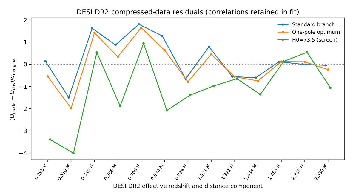
The optimized one-pole screen lowers its statistic by relative to the screen, with one additional parameter and within the specified compressed approximation. This is not evidence for a detection: the matter-density prior is derived under CDM, while the observed acoustic angle alone does not encode the full CMB anisotropy information. At , the minimum statistic is above the one-pole optimum. Omitting the matter-density prior entirely permits an essentially unchanged BAO-plus-angle statistic near with and . The resulting shift makes full CMB perturbation testing indispensable. The fixed-ruler fraction bound of Eq. (57) is conditional on a specified ratio ; it is not an unconditional lower bound for models with a high fitted .
18. Canonical Completion of the Effective Receiver Background
The homogeneous one-pole fluid admits an exact effective scalar-field reconstruction, provided it is separately conserved. Put and . Differentiating gives
The inequality follows from and . For a canonical scalar one may therefore define
These equations give and . The reconstructed stress tensor obeys its homogeneous conservation equation by construction. On any interval where , the scalar Euler–Lagrange equation follows from that conservation equation. Its rest-frame scalar propagation speed is , even though the adiabatic derivative can be negative. A barotropic-fluid interpretation with would exhibit a subhorizon gradient instability, whereas a canonical scalar does not inherit that gradient term. The field representation is an on-background effective completion of the stress tensor along the reconstructed trajectory. An off-shell equivalence, including perturbations and couplings to odd matter, is a separate dynamical specification.
Figure 4.
Reconstructed background and adiabatic derivative for the compressed-screen optimum. The canonical scalar has rest-frame ; the curves do not replace a Boltzmann perturbation calculation.
Figure 4.
Reconstructed background and adiabatic derivative for the compressed-screen optimum. The canonical scalar has rest-frame ; the curves do not replace a Boltzmann perturbation calculation.
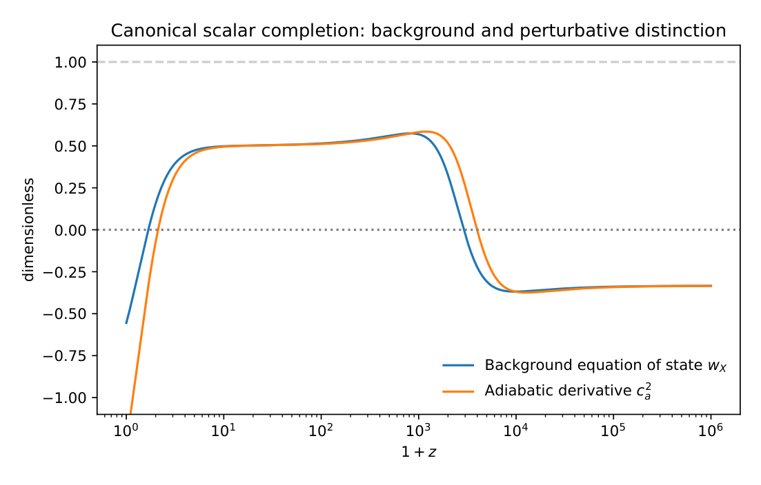
The effective single-pole susceptibility and canonical stress tensor define a cosmological response model whose physical realization is tested by perturbations and observations.
19. Additional Acoustic Bounds and Symmetry-Sector Tests
Write the sound horizon, with a common drag redshift and baryon–photon sound speed, as . For comparison against the same ordinary sources with , define the normalized reference weight
The positive receiver fraction gives at identical physical source densities, hence the following result.
Theorem 12
(Acoustic envelope and support penalty). Let . At common sound speed, drag endpoint, and ordinary source densities,
If f vanishes outside a set A of reference acoustic weight , the sharper bound holds:
Proof.
The identity follows by substituting the receiver-fraction relation into the background Hubble equation. On the support A, ; outside A the difference vanishes. Integration against the normalized nonnegative weight proves both inequalities. □
For a nominal acoustic contraction of , the unrestricted bound requires , or for the one-pole response. Concentrating the response in half of the reference acoustic weight requires . These are necessary conditions under the stated equal-source comparison, and are not CMB likelihood constraints.
Figure 5.
Universal acoustic-contraction envelope at fixed baryon–photon microphysics. The exact bound applies to the maximal fractional receiver density; a finite support interval strengthens it.
Figure 5.
Universal acoustic-contraction envelope at fixed baryon–photon microphysics. The exact bound applies to the maximal fractional receiver density; a finite support interval strengthens it.
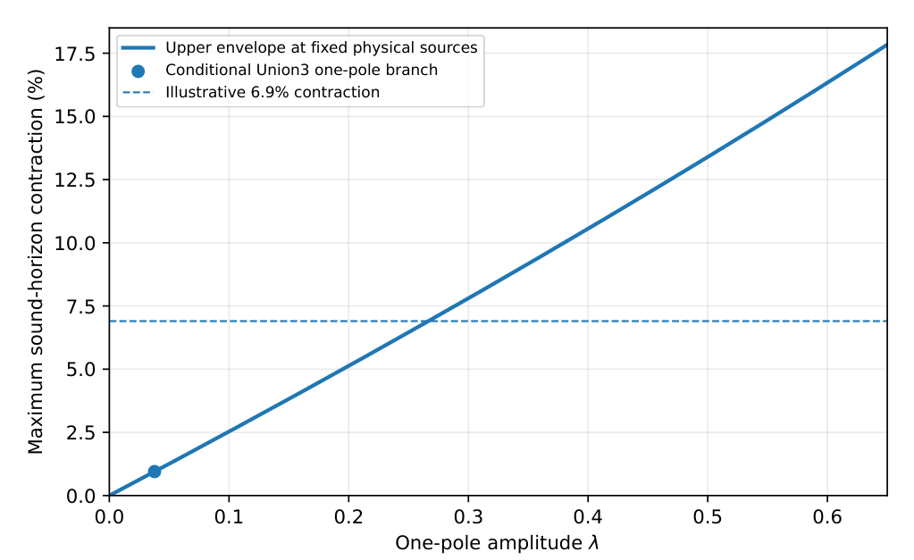
A second symmetry governs what can be inferred from homogeneous distances. Define , , and . The joint transformation
leaves the BAO ratios and the CMB acoustic angle invariant at fixed . Uncalibrated supernova magnitudes are also invariant after shifting their fitted intercept. Thus geometric measurements constrain distance shapes and products such as ; absolute calibration arises from primordial transfer physics or an independent local ruler.
20. Dark-sector Momentum Exchange and Perturbations
A separate, parity-preserving imperfect-fluid realization permits the exchange of momentum between cold dark matter and an even receiver medium. Write
The projector is orthogonal to . In the homogeneous comoving background , and the total stress tensor is covariantly conserved. The local nonrelativistic relative-velocity work is
for positive receiver enthalpy, using the orthogonal-frame linearization and a common local background. This identifies the direction of damping. In a pressureless subhorizon approximation a corresponding growth diagnostic is
Here is a coarse-grained drag rate defined by the linearized fluid model, rather than independently derived from without the enthalpies and momentum variables.
Dynamical separation.
The background reconstruction by a canonical scalar in Section ?? is the separately conserved branch, with vanishing interaction in Eq. (82). For a canonical scalar with stress tensor , its divergence is proportional to ; consequently a generic force orthogonal to the cold-dark-matter four-velocity cannot be appended to the free Klein–Gordon equation as an independent term. The momentum-exchange branch uses a receiver fluid with a specified rest-frame pressure, energy flow and viscous stress, or an explicit derivative-coupled action, together with . These two branches have different off-shell dynamics despite sharing compatible homogeneous backgrounds.
In the decoupled scalar branch, using the Newtonian-gauge potential convention when anisotropic stress is negligible, the scalar perturbation obeys
Primes denote conformal time. This source-free equation applies to the scalar realization with ; the momentum-exchange fluid instead requires its own perturbed conservation system and constitutive closure. Temperature, polarization, lensing and matter spectra are observables of the coupled Einstein–Boltzmann initial-value problem, whereas the likelihood evaluated here is a correlated geometric compression [27].
22. Results of the Spectral-Width and Resonance Tests
The positive-mixture result in Theorem 8 is independent of the numerical normalization of the reduced receiver. It is saturated in the asymptotic wings of an individual relaxation kernel and remains valid for an arbitrary positive distribution of relaxation rates. The coherent response in Theorem 9 instead achieves a narrower epoch-localized profile while retaining a globally well-defined homogeneous solution for the stated parameter region.
The two early-time benchmarks display an acoustic reduction close to seven percent with different distributions of energy between matter–radiation equality and last scattering (Table 3). The benchmarks are homogeneous acoustic calculations; multipole spectra form the separate perturbative observable. Recent precision studies of early dark energy and dark-sector transitions [10,12] provide the relevant quantitative comparison. Contemporary analyses likewise distinguish profile preferences from Bayesian evidence in dynamical-dark-energy extensions [30]. The correlated distance minimum presented above is associated with the one-pole model and the declared matter-summary prior; it is not a fit of the resonant branch. The two calculations thus constrain different physical aspects of the same phenomenological proposal.

Table 4.
Reproducible compressed-geometry screen at fixed and . The total is ; these values are not a joint CMB–BAO posterior.
Table 4.
Reproducible compressed-geometry screen at fixed and . The total is ; these values are not a joint CMB–BAO posterior.
| Case | |||||
|---|---|---|---|---|---|
| , optimized | 68.19 | 0 | 0.14074 | 0 | 16.85 |
| One-pole, optimized | 69.47 | 0.04145 | 0.14300 | 0.02072 | 10.30 |
| , optimized | 71.00 | 0.07977 | 0.14440 | 0.03988 | 17.55 |
| , optimized | 73.50 | 0.13935 | 0.14660 | 0.06967 | 59.22 |
Table 5.
Correlated geometric diagnostic. The matter-density term in the first four rows is a model-conditioned proxy. Local distance-ladder data and full CMB power spectra are excluded from this likelihood.
Table 5.
Correlated geometric diagnostic. The matter-density term in the first four rows is a model-conditioned proxy. Local distance-ladder data and full CMB power spectra are excluded from this likelihood.
| Model and condition | |||
|---|---|---|---|
| Reference branch, matter proxy | 68.12 | 0 | 44.94 |
| Receiver, fixed , matter proxy | 69.28 | 0.03776 | 39.45 |
| Receiver, free , matter proxy | 69.26 | 0.21483 | 39.41 |
| Receiver, , matter proxy | 73.50 | 0.14089 | 94.37 |
| Receiver, , no matter proxy | 73.50 | 0.22212 | 39.47 |
| Receiver, unrestricted, no matter proxy | 68.50 | 0 | 39.45 |
23. Einstein–Boltzmann Spectra of the Effective One-Pole Realization
A direct Boltzmann calculation provides an additional numerical test of the effective one-pole receiver. The separately conserved background fluid is reconstructed from the positive Friedmann branch, and its tabulated equation of state is supplied to CAMB 2.0.5. The fluid has unit rest-frame sound speed and vanishing independent anisotropic stress. The calculation is a defined phenomenological perturbative realization of the one-pole background, with an independent reference model constructed at the same Hubble constant and primordial parameters.
The comparison fixes , , , , , , and massless neutrinos. The one-pole receiver uses and . The reference sets . Both are spatially flat and use the same photon temperature and recombination prescription. A logarithmic grid of 550 scale factors spans ; the largest relative residual of the one-pole Friedmann equation is .
The receiver contracts the drag horizon by and the last-scattering sound horizon by . The equality redshift remains fixed because the physical matter and radiation densities are held equal between the two calculations. The median absolute fractional shift of the angular spectrum over is ; this is a numerical shape diagnostic rather than a goodness-of-fit statistic.
Figure 7.
CAMB temperature spectra for the fixed-parameter reference and QICT one-pole effective-fluid realization, through . The curves use identical primordial inputs.
Figure 7.
CAMB temperature spectra for the fixed-parameter reference and QICT one-pole effective-fluid realization, through . The curves use identical primordial inputs.
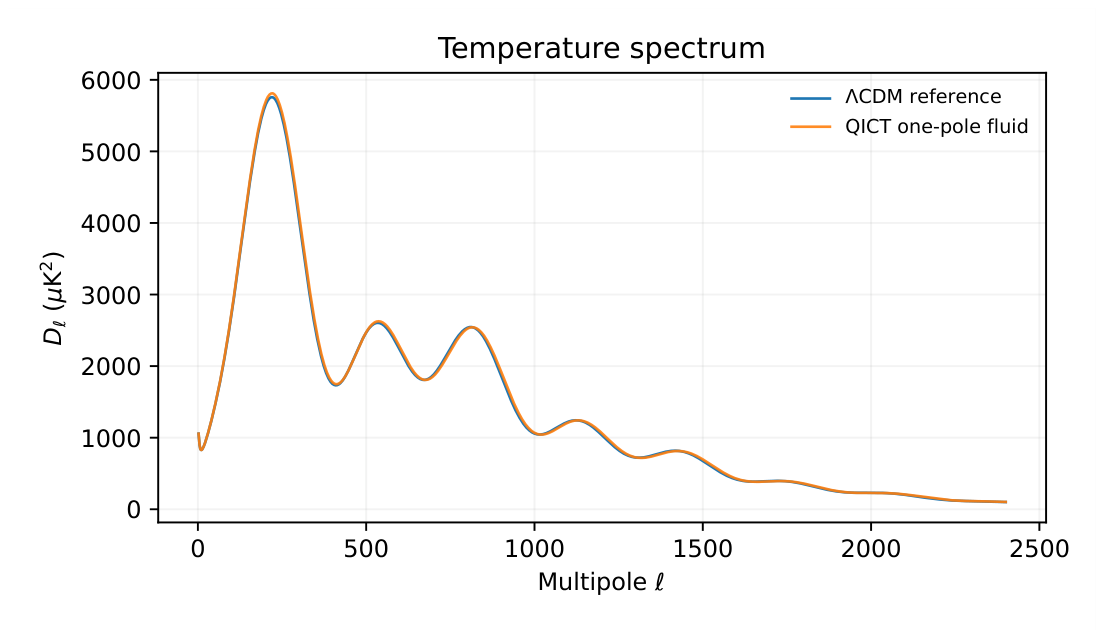
The Planck 2018 acoustic-angle summary gives [25]. The two fixed-parameter predictions in Table 6 lie on opposite sides of this value, establishing a direct numerical calibration condition for any posterior analysis of the receiver amplitude. The full , , , and lensing-potential spectra, as well as the inputs and CAMB engine version, are archived in the reproducibility package. A joint CMB likelihood and posterior inference incorporates the remaining cosmological and instrumental nuisance parameters, the calibration covariances and any specified interacting dark-matter perturbations. Online Resource 4 documents the exact benchmark and its physical scope.
24. Conserved Energy, Hilltop Activation and the Criteria for Cosmological Closure
The quantum receiver, passive-response backgrounds and finite-charge action have different starting data (Table 1). Their common physical implications can be assessed through three independent tests: parity selection of the dark excitation, gravitational conservation of the total additional sector, and dynamical preparation of a sufficiently short-lived early contribution. Details of the phase-space searches, microscopic matching conditions and quantum kinetic closure are provided in Supplementary Sections ??, ?? and ??.
24.1. A Model-Independent Exit Condition
Let denote the complete extra phase-plus-odd sector and let be a separately conserved reference background. If the internal energy transfer is reciprocal, the total equation obeys , where a prime is . Define , and . Integrating the continuity equation gives the exact relation
Solving Eq. (87) for at the final interval gives
This necessary condition is independent of the partition of the additional energy between interacting daughters as long as its total stress tensor is conserved. With matter–radiation equality fixed at , the screening values at and at require . This is a condition on the specified additional positive component, not a cosmological posterior. In particular, conversion into cold parity-odd particles is not a loss term in Eq. (87). The detailed transfer solution shows that even an initially stiff parent fails this particular screening target if its constant conversion rate exceeds (Supplementary Section ??). If the odd contribution replaces reference cold matter rather than augmenting it, the background decomposition and the test must be reformulated.
24.2. Dynamical Onset and the Earlier Energy Budget
For the finite-charge action in Eq. (3), the hilltop at has energy . Its canonical longitudinal and transverse squared growth rates are
where denotes the finite charge and is unrelated to the e-fold variable N of Eq. (87). Both are positive; the longitudinal instability is faster. In an unperturbed radiation-era background the normalized regular linear solution is . The exact symmetric configuration with zero velocity does not activate spontaneously under deterministic classical evolution. A displacement, a physically specified preparation mechanism and nonlinear propagation are required. The canonical Hessian, Bessel solution and the full transverse analysis are derived in Supplementary Sections ?? and ??.
The numerical two-phase scans provide examples with sufficiently rapid late dilution, but not an independent selection of their high-redshift initial state. A separate lower bound applies to an initially positive, separately conserved canonical phase sector: for , . At and the reference parameters above, this is ; hence a requirement below at that redshift cannot be met within that specified comparison. The bound does not extend unchanged to a signed difference relative to replaced reference matter. Details, trajectory scans and sensitivity tests appear in Supplementary Section ??.
24.3. What Each Numerical Test Establishes
Table 7.
Interpretation of the independently derived and executed tests. A numerical response is a physical prediction only within the specified model, state and normalization.
Table 7.
Interpretation of the independently derived and executed tests. A numerical response is a physical prediction only within the specified model, state and normalization.
| Test | Physical inference |
|---|---|
| Parity and spectral criteria | Exact conditional selection rules; physical particle identification further needs a thermodynamic pole, dispersion and calibrated clock. |
| Finite-charge homogeneous evolution | Exact equations, hilltop curvatures and conditional initial-value solutions; no dynamical initial-state selection. |
| Receiver distance and CAMB benchmarks | Geometric identifiability and fixed-input acoustic/transfer responses; not a calibrated likelihood for the interacting two-phase action. |
| Regulated classical and quantum energy transfer | Reciprocal conservation and cutoff sensitivity; no cutoff-independent absolute odd-particle abundance or vacuum-energy selection. |
A decisive model comparison would require the microscopic Hamiltonian and physical state, pole and mass calibration, renormalized gravitational source, coupled Einstein–Boltzmann perturbations, and a common likelihood with a reoptimized CDM reference. The necessary conditions are precise; the present geometric and fixed-fluid benchmarks do not establish that entire chain.
25. Discussion
The three constructions lead to rigorous, but different, claims. At the operator level, parity determines selection rules and positive spectral measures constrain candidate excitations. At the level of an effective particle theory, the same symmetry permits a continuous range of positive masses (Proposition 1); at fixed dynamics, even states may have different occupations (Proposition 5). These are not failures of parity protection. They identify two independent pieces of physical input that a microscopic model must supply before it can predict a dark-matter mass and relic abundance.
The gravitational receiver has similarly precise conditions. Diffusion gives an operational registration time; the cutoff inequality bounds a positive source but leaves its saturation fraction undetermined. A specified passive constitutive law then yields an unambiguous Friedmann branch and acoustic kernel. The logarithmic-width bound constrains positive mixtures of relaxation rates, whereas a coherent resonance provides a different response class. Neither result shows that the finite-charge phase fluctuations reproduce the same susceptibility. Establishing that connection requires a calculated retarded correlator, a source-normalization prescription and consistent perturbations.
The covariant action supplies a separate, fully specified classical test. Its phase metric is positive, its potential determines the hilltop curvatures, and a symmetric displacement grows analytically in radiation domination. Nonlinear integrations display conditional histories with rapid later dilution, but a high-redshift preparation is part of the dynamics and must be checked independently. The exact energy ledger is particularly restrictive: producing stable cold odd quanta cannot remove their contribution to the total Friedmann source. For the declared additional-component benchmark, the integrated-pressure threshold and the earlier-epoch bound must be satisfied simultaneously. A compensating replacement of reference matter constitutes a different model and cannot be assessed with the unchanged bound.
The ultraviolet and observational studies delimit what can currently be inferred. The matched odd Gaussian determinant is finite at constant phase gradient after three subtractions, and its curved-background divergence identifies necessary local counterterms. This does not determine their finite gravitational coefficients or renormalize the full interacting theory. The DESI DR2–Union3 screen tests the separately defined one-pole background. Its improvement over a reoptimized nested CDM model disappears when the reference-conditioned matter prior is removed. Fixed-input CAMB spectra reveal perturbative differences in one canonical-fluid completion, but the action has not been subjected to a common native Planck–ACT–DESI likelihood. The decisive link is a regulator-controlled quantum state and stress tensor evolved through the coupled Einstein–Boltzmann system, followed by independent optimization of both cosmological hypotheses. Supplementary Sections ??, ?? and ?? provide the corresponding analytical obstructions and executed sensitivity tests.
26. Conclusions
The dark-sector construction admits sharp results at three levels: excitation symmetry, covariant phase dynamics and cosmological energy accounting. Conserved parity gives exact selection rules and conditionally protects the lightest odd asymptotic state. A positive odd-sector spectral measure constrains the candidate particle pole, while an explicit invariant scalar family shows that its mass is not selected by symmetry alone. At fixed quadratic dynamics, parity-even quantum states can carry different odd-particle occupations. Mass and relic density therefore remain distinct quantities to be fixed by a microscopic spectrum and a specified physical state.
For the two-phase covariant action, the symmetric hilltop has two unstable canonical directions with analytic growing solutions in a radiation background. Their existence establishes a dynamical instability, not automatic preparation of a cosmological transition. More decisively, conservation of the combined phase and odd-particle sector yields an exact constraint on its dilution. For the stated positive-component benchmark, a decrease from at to at most at requires . Transfer into stable cold daughters cannot evade that bound; earlier energy constraints restrict the admissible initial histories further.
The passive-receiver analysis provides additional spectral-width and acoustic bounds for explicitly defined effective responses. Correlated DESI DR2–Union3 distances and fixed-input CMB calculations test these responses within their respective approximations. The compressed-fit preference depends on an imported CDM-conditioned matter prior and does not establish a preference for the covariant finite-charge action. Likewise, the Gaussian one-loop counterterms are a controlled ultraviolet result, not a renormalization of the complete interacting gravitational theory.
The central outcome is a set of mathematical and numerical criteria that distinguish a protected dark excitation from a predicted dark-matter population and a consistent cosmological source. Completing their connection requires one microscopic generator to determine the physical pole and state, a renormalized stress tensor for the same action, and coupled perturbations tested against a common full likelihood. The present results make each of those physical identifications explicit and independently testable.
Supplementary Materials
The following supporting information can be downloaded at the website of this paper posted on Preprints.org. The accompanying QICT Technical Supplement contains the curved-space one-loop counterterms, initial-state non-uniqueness theorem, extended receiver-source matching, three-sector and quantum-kinetic analyses, the original mathematical appendices and complete spectral, backreaction and phase-activation derivations. Additional technical studies (Online Resources 2–4 and Supplements K–M, W–Y and AD–AM), numerical source files, input covariances, benchmark spectra and execution records are supplied in the archive. The figure and data indices identify the corresponding source for every reported numerical experiment.
Author Contributions
Mohamed SACHA: conceptualization, methodology, mathematical formulation, investigation, formal analysis, manuscript development and scientific supervision.
Funding
corresponding author to confirm before submission
Institutional Review Board Statement
Not applicable. This work is a theoretical and computational cosmological analysis involving no human participants or animals.
Informed Consent Statement
Not applicable.
Data Availability Statement
The reproduction package includes analytic kernel and acoustic-envelope tests, together with the DESI DR2 and Union3 compressed inputs used in the reported calculations, including the within-survey covariance representations, together with scripts, plots, derived tables, fixed-input CAMB spectra and symbolic-identity checks. Original observational measurements should be obtained from the cited collaborations; their licensing and covariance conventions take precedence. The cosmology-specific source code and theoretical checks are provided in the accompanying ZIP archive. The additional Planck–DESI QICT fixed-point comparison is separately identified in the source provenance and was not fitted with the two-phase action.
Conflicts of Interest
corresponding author to confirm before submission.
References
- Bisio, A.; D’Ariano, G.M.; Tosini, A. Dirac Quantum Cellular Automaton in One Dimension: Zitterbewegung and Scattering from Potential. Phys. Rev. A 2013, 88, 032301. [Google Scholar] [CrossRef]
- Pérez, A. Asymptotic Properties of the Dirac Quantum Cellular Automaton. Phys. Rev. A 2016, 93, 012328. [Google Scholar] [CrossRef]
- Raynal, P. Simple Derivation of the Weyl and Dirac Quantum Cellular Automata. Phys. Rev. A 2017, 95, 062344. [Google Scholar] [CrossRef]
- Bisio, A.; D’Ariano, G.M.; Perinotti, P. Special Relativity in a Discrete Quantum Universe. Phys. Rev. A 2016, 94, 042120. [Google Scholar] [CrossRef]
- D’Ariano, G.M.; Perinotti, P. Derivation of the Dirac Equation from Principles of Information Processing. Phys. Rev. A 2014, 90, 062106. [Google Scholar] [CrossRef]
- Blekherman, G.; Kummer, M.; Riener, C.; Schweighofer, M.; Vinzant, C. Generalized Eigenvalue Methods for Gaussian Quadrature Rules. Ann. Henri Lebesgue 2020, 3, 1327–1341. [Google Scholar] [CrossRef]
- Hansen, M.; Lupo, A.; Tantalo, N. Extraction of Spectral Densities from Lattice Correlators. Phys. Rev. D. 2019, 99, 094508. [Google Scholar] [CrossRef]
- Lupo, A.; Tantalo, N. Extraction of Spectral Densities from Lattice Correlators: Decoupling Signal from Noise. Phys. Rev. D. 2026, 114, 074511. [Google Scholar] [CrossRef]
- Abdul Karim; M.; et al. (DESI Collaboration); et al. DESI DR2 Results II: Measurements of Baryon Acoustic Oscillations and Cosmological Constraints. Phys. Rev. D. 2025, 112, 083515. [Google Scholar] [CrossRef]
- Poulin, V.; Smith, T.L.; Calderón, R.; Simon, T. Impact of ACT DR6 and DESI DR2 for Early Dark Energy and the Hubble Tension. Phys. Rev. D. 2026, 113, 063519. [Google Scholar] [CrossRef]
- Reeves, A.; Ferraro, S.; Nicola, A.; Refregier, A. Multiprobe Constraints on Early and Late Time Dark Energy. Phys. Rev. D. 2026, 113, 103512. [Google Scholar] [CrossRef]
- Garny, M.; Niedermann, F.; Rubira, H.; Sloth, M.S. Hot New Early Dark Energy: Dark Radiation Matter Decoupling. Phys. Rev. D. 2026, 114, 043532. [Google Scholar] [CrossRef]
- Hoelscher, Z.J.; Kephart, T.W.; Scherrer, R.J.; Holley-Bockelmann, K. Partial Relief of the Hubble Tension and a Natural Self-Interacting Dark Matter Candidate from Staged Symmetry Breaking. Phys. Rev. D. accepted. 2026. [Google Scholar] [CrossRef]
- Goldstein, S.; Hill, J.C. 2% Determination of Neff from Primordial Element Abundance, Cosmic Microwave Background, and Baryon Acoustic Oscillation Measurements. Phys. Rev. D. 2026, 114, L021305. [Google Scholar] [CrossRef]
- Rubin, D.; et al. Union through UNITY: Cosmology with 2000 SNe using a unified Bayesian framework. Astrophys. J. 2025, 986, 231. [Google Scholar] [CrossRef]
- Lindblad, G. On the generators of quantum dynamical semigroups. Commun. Math. Phys. 1976, 48, 119–130. [Google Scholar] [CrossRef]
- Breuer, H.-P.; Petruccione, F. The Theory of Open Quantum Systems; Oxford University Press: Oxford, 2002. [Google Scholar]
- Manzano, D. A Short Introduction to the Lindblad Master Equation. AIP Adv. 2020, 10, 025106. [Google Scholar] [CrossRef]
- Wootters, W.K.; Zurek, W.H. A Single Quantum Cannot Be Cloned. Nature 1982, 299, 802–803. [Google Scholar] [CrossRef]
- Cohen, A.G.; Kaplan, D.B.; Nelson, A.E. Effective Field Theory, Black Holes, and the Cosmological Constant. Phys. Rev. Lett. 1999, 82, 4971–4974. [Google Scholar] [CrossRef]
- Zaborowski, E.A.; et al. H0 without the Sound Horizon (or Supernovae): A 2% Measurement in DESI DR1. JCAP 2026, 04, 004. [Google Scholar] [CrossRef]
- Courbin, F.; Maeder, A. The Hubble Tension in Light of the Symmetry of Scale Invariance. Symmetry 2026, 18, 207. [Google Scholar] [CrossRef]
- Zhou, Z.; Wang, S.; Miao, Z.; Ai, C.; Zhang, H. Geometric Obstruction to Resolving the Hubble Tension: Orthogonality of Scale and Shape in Distance Measurements. Phys. Rev. D. 2026, 114, 063511. [Google Scholar] [CrossRef]
- Ma, C.-P.; Bertschinger, E. Cosmological Perturbation Theory in the Synchronous and Conformal Newtonian Gauges. Astrophys. J. 1995, 455, 7–25. [Google Scholar] [CrossRef]
- Planck Collaboration. Planck 2018 Results. VI. Cosmological Parameters. Astron. Astrophys. 2020, 641, A6. [Google Scholar] [CrossRef]
- H0 Distance Network Collaboration. The Local Distance Network: A Community Consensus Report on the Measurement of the Hubble Constant at ∼1% Precision. Astron. Astrophys. 2026, 708, A166. [Google Scholar] [CrossRef]
- Blas, D.; Lesgourgues, J.; Tram, T. The Cosmic Linear Anisotropy Solving System (CLASS). Part II: Approximation schemes. J. Cosmol. Astropart. Phys. 2011, 07, 034. [Google Scholar] [CrossRef]
- Davies, R.B. Hypothesis testing when a nuisance parameter is present only under the alternative. Biometrika 1977, 64, 247–254. [Google Scholar] [CrossRef]
- Self, S.G.; Liang, K.-Y. Asymptotic Properties of Maximum Likelihood Estimators and Likelihood Ratio Tests under Nonstandard Conditions. J. Am. Stat. Assoc. 1987, 82, 605–610. [Google Scholar] [CrossRef]
- Lozano Torres, J.A. Dynamical Dark Energy from DESI DR2 and DES Year 6 BAO, Supernovae, and Cosmic Chronometers: A 3σ Preference without Decisive Bayesian Evidence. MNRAS 2026, 551, 4. [Google Scholar] [CrossRef]
- Margolus, N.; Levitin, L.B. The Maximum Speed of Dynamical Evolution. Physica D. 1998, 120, 188–195. [Google Scholar] [CrossRef]
- Bella, M.; Poulin, V.; Vagnozzi, S.; Knox, L. Double the axions, half the tension: multi-field early dark energy eases the Hubble tension. arXiv:2604.13535. 2026. Available online: https://arxiv.org/abs/2604.13535.
- Hall, L.J.; Jedamzik, K.; March-Russell, J.; West, S.M. Freeze-in Production of FIMP Dark Matter. JHEP 2010, 03, 080. [Google Scholar] [CrossRef]
- SPT-3G Collaboration. SPT-3G D1: CMB Temperature and Polarization Power Spectra and Cosmology from 2019 and 2020 Observations of the SPT-3G Main Field. Phys. Rev. D. 2026, 113, 083504. [Google Scholar] [CrossRef]
- Pollak; W.; et al. (SPT-3G Collaboration); et al. SPT-3G D1: Quadratic-Estimator CMB Lensing Reconstruction and Cosmology. arXiv. 2026. Available online: https://arxiv.org/abs/2608.31136.
- Calabrese, E.; et al. The Atacama Cosmology Telescope: DR6 Constraints on Extended Cosmological Models. JCAP 2025, 11, 063. [Google Scholar] [CrossRef]
- Kofman, L.; Linde, A.; Starobinsky, A.A. Towards the Theory of Reheating after Inflation. Phys. Rev. D. 1997, 56, 3258–3295. [Google Scholar] [CrossRef]
- Baacke, J.; Heitmann, K.; Pätzold, C. Nonequilibrium Dynamics: A Renormalized Computation Scheme. Phys. Rev. D. 1997, 55, 2320. [Google Scholar] [CrossRef]
- Baacke, J.; Heitmann, K.; Pätzold, C. Renormalization of Nonequilibrium Dynamics in FRW Cosmology. Phys. Rev. D. 1997, 56, 6556. [Google Scholar] [CrossRef]
- Berges, J. Introduction to Nonequilibrium Quantum Field Theory. AIP Conf. Proc. 2004, 739, 3–62. Available online: https://arxiv.org/abs/hep-ph/0409233. [CrossRef]
- Khlebnikov, S.Y.; Tkachev, I.I. Classical Decay of the Inflaton. Phys. Rev. Lett. 1996, 77, 219. [Google Scholar] [CrossRef]
- Kainulainen, K.; Nurmi, S.; Väisänen, O. Tachyonic Production of Dark Relics: Classical Lattice vs. Quantum 2PI in Hartree Truncation. JHEP 2024, 10, 009. [Google Scholar] [CrossRef]
- Figueroa, D.G.; Florio, A.; Torrenti, F.; Valkenburg, W. CosmoLattice: A Modern Code for Lattice Simulations of Scalar and Gauge Field Dynamics in an Expanding Universe. Comput. Phys. Commun. 2023, 283, 108586. [Google Scholar] [CrossRef]
- Weinberg, S. The Cosmological Constant Problem. Rev. Mod. Phys. 1989, 61, 1–23. [Google Scholar] [CrossRef]
- Gondolo, P.; Gelmini, G. Cosmic Abundances of Stable Particles: Improved Analysis. Nucl. Phys. B 1991, 360, 145–179. [Google Scholar] [CrossRef]
- Meng, G.; Liu, C. Volume Dependence of Spectral Weights for Unstable Particles in a Solvable Model. Phys. Rev. D. 2008, 78, 074506. [Google Scholar] [CrossRef]
- Lüscher, M. Volume Dependence of the Energy Spectrum in Massive Quantum Field Theories. I. Stable Particle States. Commun. Math. Phys. 1986, 104, 177–206. [Google Scholar] [CrossRef]
- Sobczyk, J. E.; Roggero, A. Spectral Density Reconstruction with Chebyshev Polynomials. Phys. Rev. E 2022, 105, 055310. [Google Scholar] [CrossRef]
Figure 6.
Sensitivity of the geometric receiver profile to the width of an externally imposed matter-density summary. The horizontal coordinate is an assumed prior width, not a CMB-derived uncertainty within QICT.
Figure 6.
Sensitivity of the geometric receiver profile to the width of an externally imposed matter-density summary. The horizontal coordinate is an assumed prior width, not a CMB-derived uncertainty within QICT.
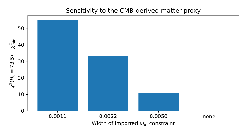
Table 1.
Logical domain of each QICT realization. A microscopic pole mass, absolute gravitational vacuum term, or a global CMB likelihood is a derived quantity only after the additional physical inputs are specified and independently tested.
Table 1.
Logical domain of each QICT realization. A microscopic pole mass, absolute gravitational vacuum term, or a global CMB likelihood is a derived quantity only after the additional physical inputs are specified and independently tested.
| Construction | Independent mathematical input | Established output |
|---|---|---|
| Parity-graded sector | Conserved grading and positive physical energy | Odd-state selection and stability |
| Causal receiver response | Passive susceptibility and background density map | Friedmann and acoustic bounds |
| Finite-charge covariant action | Integer N, F, and initial state | Vacuum curvatures; conditional trajectories |
| Quantum mode and covariance systems | Regulator, state and approximation order | Finite-cutoff quantum backreaction |
| Geometric and Boltzmann benchmarks | Compressed survey data or fixed fluid inputs | Restricted fits; reference multipoles |
Table 2.
Conditional acoustic benchmark, fixed baryon loading and drag redshift. The ratio is used only as a numerical ruler proxy, not as a CMB-derived posterior for this model.
Table 2.
Conditional acoustic benchmark, fixed baryon loading and drag redshift. The ratio is used only as a numerical ruler proxy, not as a CMB-derived posterior for this model.
| Reduction (%) | |||
|---|---|---|---|
| 0.2000 | 0.1000 | 0.96949 | 3.051 |
| 0.4000 | 0.2000 | 0.93739 | 6.261 |
| 0.43842 | 0.21921 | 0.93102 | 6.898 |
| 0.6000 | 0.3000 | 0.90343 | 9.657 |
Table 3.
Fixed-source acoustic benchmarks computed from the implicit Friedmann equation. The physical baryon and radiation densities, and are held fixed. These are homogeneous tests rather than CMB anisotropy fits.
Table 3.
Fixed-source acoustic benchmarks computed from the implicit Friedmann equation. The physical baryon and radiation densities, and are held fixed. These are homogeneous tests rather than CMB anisotropy fits.
| Response | Peak f | |||
|---|---|---|---|---|
| Single relaxation pole () | 0.2193 | 0.1091 | 0.1817 | 0.06900 |
| Collective resonance (, ) | 0.3000 | 0.1749 | 0.0639 | 0.06881 |
Table 6.
Direct CAMB 2.0.5 output for a fixed-parameter comparison. The entries are numerical predictions of the two specified effective-fluid models, rather than fitted posterior values.
Table 6.
Direct CAMB 2.0.5 output for a fixed-parameter comparison. The entries are numerical predictions of the two specified effective-fluid models, rather than fitted posterior values.
| Quantity | Reference CDM | QICT one-pole fluid |
|---|---|---|
| (Mpc) | 147.3746 | 146.5443 |
| (Mpc) | 144.7086 | 143.8873 |
| 1.044303 | 1.038441 | |
| 1089.8144 | 1089.9092 | |
| 3378.9716 | 3378.9716 |
Disclaimer/Publisher’s Note: The statements, opinions and data contained in all publications are solely those of the individual author(s) and contributor(s) and not of MDPI and/or the editor(s). MDPI and/or the editor(s) disclaim responsibility for any injury to people or property resulting from any ideas, methods, instructions or products referred to in the content. |
© 2026 by the authors. Licensee MDPI, Basel, Switzerland. This article is an open access article distributed under the terms and conditions of the Creative Commons Attribution (CC BY) license (http://creativecommons.org/licenses/by/4.0/).
Copyright: This open access article is published under a Creative Commons CC BY 4.0 license, which permit the free download, distribution, and reuse, provided that the author and preprint are cited in any reuse.