Submitted:
27 January 2026
Posted:
28 January 2026
You are already at the latest version
Abstract
Periodic supercell lattice structures with elements of random polydispersity disorder were created, to simulate the effect of randomization on photonic crystals, using finite-difference time domain (FDTD) methods. As a key exemplar system, a three-dimensional “inverse opal” structure of a face-centered cubic lattice with air spheres in a silicon dielectric was simulated, with sphere radii within supercells following a randomized Gaussian distribution, with characteristic standard deviation and mean. A corresponding ordered lattice with a bandgap with magnitude 3.5% of the normalized frequency range was used as a direct control, with sphere radius 0.34 times the lattice constant a. For a range of standard deviations, up to 5.9% of the 0.34a mean, a Monte-Carlo style approach was adopted, with photonic band properties analyzed over a large number of repeat simulations to ensure statistical significance. The corresponding Gaussian distribution in the resultant photonic bandgap magnitudes is broadened with increasing polydispersity such that an evolving fraction of simulations no longer exhibits a non-zero bandgap. A characteristic pseudo-transition occurs at a standard deviation of approximately 4.1% of the 0.34a mean, above where the frequency of simulations still returning a finite bandgap rapidly diminishes. Some isolated configurations, with a high degree of uniqueness, can exhibit enhanced bandgap properties (greater than the 3.5% benchmark) despite considerable polydisperse disordering; and we envisage that these findings point towards the use of engineered randomness in supercell systems to create desired photonic crystal properties and functionality, such as localization and optical bandgaps.
Keywords:
photonic crystals
; disorder
; bandgaps
; finite-difference time domain simulations
1. Introduction
Photonic crystals (PCs), or photonic bandgap (PBG) crystals, are periodic dielectric materials that are designed to control how electromagnetic waves propagate [1]. The crystal is designed to prevent or inhibit the propagation of light at certain frequencies, either through photonic bandgaps or by significantly modifying the density of electromagnetic states [2,3,4]. PCs are an area of active research, with strong emphases on both two-dimensional and three-dimensional PCs for their many practical uses, such as communication [5], computing [6,7] and materials science [8,9]. Photonics, more widely, is the control of photons in free space or matter, in analogy to the control of electron-charge seen in electronics [10]. The most widespread use of photonics at present is for telecommunications through the optical fiber waveguide [11,12], which allows for data transfer at much higher bandwidth, higher efficiency, and lower cost than equivalent electronic communications methods. Optical computing, also called photonic computing, is another future application of photonics that proposes using light rather than electrons as the medium for computers for the similar reasons [13]. PCs constructed with bandgaps to control the propagation of certain frequencies would be the foundation to such photonic computers [14,15].
Recent research has sparked interest into the effects of structural disorder within Photonic crystals. Studies focused on biological and biomimetic materials [16,17,18], reveal that such disorder can exert both positive and negative influence on the efficacy of light propagation in these structures. Whether light localizes or delocalizes hinges on the specific disorder introduced. The extrinsic introduction of disorder into photonics, and the engineering of topologies associated with disordered structures [19], has revealed new ways for manipulating the light spectrum, transport, and wavefront properties [20,21,22]. These variations can also lead to unique optical properties and functionalities not present in perfectly ordered PCs. For instance, the disorder can facilitate the phenomenon of Anderson localization of light, where light waves are trapped and localized due to scattering from random defects in the crystal structure, or irregularities in the crystal lattice [23,24]. Notably, the utilization of materials lying along the spectrum between the regimes of perfect order and disorder shows promise in yielding innovative optical phenomena [25,26]. The simulation of disorder in photonic crystals aids in comprehending its impact on light propagation and in the design of materials with tailored optical properties. Using self-stabilized colloid deposition, scalable methods to fabricate tailored disorder have been presented [27], this allowed control over lateral and vertical statistics of the patterns and accurate prediction of particle patterns is investigated using structure factor and optical measurements.
In this paper, the effect of randomization disorder on photonic crystals was simulated using the Massachusetts Institute of Technology (MIT) Electromagnetic Equation Propagation (MEEP) and Photonic Bands (MPB) open source freewares aimed at simulating Maxwell’s equations, where the evolution of electromagnetic waves over time is modelled in materials [28,29]. The output from MEEP and MPB was confirmed to match expected results using photonic crystal unit cells (fcc lattices of packed spheres) with known band structures from literature. Supercell structures were created, with significant variations in the radius size added as an element of disorder.
Three-dimensional inverse opal structures (see Figure 1) of a face-centered cubic (fcc) lattice with air spheres in a dielectric, are simulated both in the ordered state and with a randomization of the sphere radii. A fcc unit cell known to have a bandgap of 3.5% (of normalized frequency range) in the ordered configuration, with sphere radius 0.34a where a is the lattice constant, was used as the reference. The sphere radii are then randomized according to a Gaussian distribution, with a mean radius μ /a = 0.34. Multiple standard deviations (σ) were used in simulations, ranging from σ/a = 0.0025 (~0.7% of 0.34a) to σ/a = 0.020 (~5.9%). In order, to generate a statistically significant body of outputs, ~500 independent simulations runs were executed for each value of σ studied.
A reduced prevalence and width of the bandgap in 3D systems with a small variance disorder was shown and is expected [30] and shows that the introduction of random disorder has a crucial influence on the maintenance and degradation of PBGs. However, some PBGs were shown to be larger than the ordered configuration. This ability to use engineered disorder to create tailored optical bandgap properties, following the outputs of simulation, is of particular interest and warranting of further investigation and future optimization.
2. Materials and Methods
The MEEP software package for Python (v1.29.0), installed on Linux Ubuntu 22.04, was used to generate all the reported simulations. NumPy was used extensively throughout, as well as Matplotlib for general data plots and VisPy for 3D plots. An AMD Ryzen 7 processor with 32GB RAM was used for development, while simulations were performed on an Intel i7 processor and with the use of Supercomputing Wales. Both systems produced numerical results identical to within the pertinent number of significant figures.
2.1. Simulation Software
MEEP and MPB are a bundled set of free open-source software for simulating electromagnetics in materials. MEEP is specialized for time domain simulations using the finite-difference time domain (FDTD) method, where it simulates how electromagnetic waves evolve over time in a material [28,31]. FDTD is a numerical analysis method for solving computational electrodynamics; Maxwell’s equations are replaced by a set of finite difference equations, such as Δf = f(x + 1) − f(x), and then these are solved for given boundary conditions and appropriate field points [32].
MEEP and MPB do not use standard SI units [31,33]. Instead, they use a set of scale-invariant dimensionless units where c = 1. The frequency f is given in normalized units of c/a (and angular frequency ω in 2πc/a). MPB outputs the frequencies from 0 to c/a in the Brillouin zone. Hence, supposing if MPB showed a bandgap at f = 0.5 c/a, and the lattice constant was known to be a = 250 nm, the bandgap would be at f = 600 THz or wavelength λ = 500 nm.
MPB specializes in frequency solving, especially for band structures, in PCs [29,33]. Central to both MEEP and MPB is the ’geometry’ variable, which predictably specifies the physical geometry simulated. In MEEP, it primarily affects how electromagnetic waves propagate through the cell, while in MPB, combined with the ’geometry lattice’ variable, it specifies the periodicity of photonic crystals. The Brillouin zone of the crystal is described through the ’k-points’ variable in values of 2π/a.
2.2. Three-Dimensional Systems
The system chosen for this investigation was fcc lattices of packed spheres in general and inverse opal structures [34] in particular. A silicon-based inverse opal structure with air sphere radius r/a = 0.34 was used as the primary structure to determine how randomized variance in radius influenced the bandgap. Simulations of three-dimensional supercells were highly constrained by processing power. The time taken to compute a single band diagram is strongly dependent on the number of bands calculated, and the number of bands that need to be calculated significantly increases based on the size of the supercell. The silicon-based inverse opal supercell used was 2 x 2 x 2, for a total of 8 air spheres in the silicon material, enabling a larger number of simulations and this a larger sample size, within reasonable constraints of computing time. However, of note, the small size of the supercell (2 x 2 x 2) is nonetheless a good representation of all the nearest neighbor lattice interactions. An initial calibration cell was calculated with constant air sphere radius r/a = 0.34 to determine the number of bands needed to be calculated and was found to be about 150 bands.
A Gaussian distribution was used to allocate the radii of the air spheres within each independent simulation run. In order to maintain physically realistic outputs, the upper limit was set to radius r/a = 1/√8 ≈ 0.354 so the spheres cannot spatially overlap, with a lower distribution limit of r/a = 0.30. The median radius was selected to be μ /a = 0.34 with a standard deviation σ. These parameters were used to create an array of eight values, which was then used to overwrite the sphere radii in the original supercell, with the randomly assigned radii thus updated for each successive simulation run. Hence, outputs are collected in a “Monte Carlo” fashion from many multiple independent simulations.
Multiple standard deviation values were investigated to compare how the deviation of sphere radii, representing the physical disordering, affects the PBG. The target number of simulations for each value of σ was ~500 to produce statistically significant results. The largest deviation was chosen to be σ/a = 0.020, approximately 5.9% of the mean 0.34a. The smallest deviation was σ/a = 0.0025 (0.7% of the mean). A key range of interest for values in between was chosen based on the results produced, with a focus on deviations between σ/a = 0.0075, ~2.4% of the mean, and σ/a = 0.010, ~2.9% of the mean.
3. Results
3.1. Uniform Cells
As described, the calculations were validated using a unit cell with a known bandgap [1] for a given radius r/a = 0.34 and comparing to the uniform 2 x 2 x 2 supercell. The matrix material has dielectric constant ε = 13 (silicon) and the spheres ε = 1 (air). These two baseline simulations produced identical results to within three significant figures, a bandgap of 3.50% in frequency. Variation beyond these significant figures is attributable to the inherent uncertainty in the calculations. Identical simulations with no parameters changed showed variation beyond the three significant figures. Figure 2 shows the band structures, with Figure 2a showing the unit cell and Figure 2b showing the supercell. The supercell has significant band folding, resulting in a very dense band diagram compared to the unit cell.
3.2. Radii and Bandgap Distributions
All radii values produced for each standard deviation of radii σ were plotted in Figure 3 in a fifty-bin histogram, within the physically limited range of 0.30 < r/a ≤ 0.354 to show the overall distribution for each deviation. Each simulation produced eight radii values, and the overall shapes align with the expected Gaussian distributions. The narrower distributions are notably sharper than the broader distributions, resulting in a non-uniform y-axis scaling.
The bandgap magnitudes (by bandgap percentage) were likewise sorted into fifty-bin histograms, plotted in Figure 4. These were plotted against the frequency of simulation occurrences. A dotted black line marks the size of the uniform cell bandgap of 3.5%. The frequency of the zero bin (bandgap = 0%) increases sharply as σ increases, resulting in very “squashed”-appearing plots. A Gaussian line-fit, shown as solid blue lines, was applied to the histograms, excluding the zero bin, for all plots that showed a clear Gaussian shape. Figure 4h, σ/a = 0.015, and Figure 4i, σ/a = 0.020, did not fit such a Gaussian curve, and the mean bandgap percentage, Μ, is notionally ≤ 0. The parameters of the Gaussian fits (Μ and the standard deviation Σ) are collated in Table 1.
The MPB documentation [33] states that bandgaps of less than 1.0% are considered within the bounds of uncertainty and can represent false gaps produced by uncertainty in the calculation or the crossing of two frequency bands. This was not considered in plotting the histograms or in Table 1, although the general reliability of Gaussian fitting in Figure 4 suggest this is not a significant problem. The MPB documentation does suggest ways of interrogating suspected false gaps by targeting the specific frequency bands individually, but this was not done due to the large number of simulations produced.
In terms of the general trends observed for these inverse opal supercell lattices, the mean bandgap magnitude by percentage (Μ) increased with decreasing disorder from sphere polydispersity (σ) while the corresponding standard deviation (Σ) decreased with decreasing σ, shown in Table 1 and Figure 5. The errors in Μ, Σ were calculated using a standard error, where the mean and standard deviation of the Gaussian fit were divided by the square root of the number of simulations. A simple linear extrapolation of the plots in Figure 5a gives an inferred Μ = 0 intercept between σ/a = 0.013 and 0.015, and corresponding Σ value exceeding 1.5%. This is strongly corroborated in Figure 5c, where the cumulative fraction of simulations with non-zero bandgap (Ω) can be intuitively fitted to a sigmoidal function, with Ω tending to 1 as σ/a approaches zero and tending to 0 as σ/a becomes large. The half-height (Μ = 0.5) point of the trendline is found to be at σ/a = 0.014, determining a point at which there is quite a rapid pseudo-transition from a regime whereby bandgaps are mostly present in simulations to one where they are predominantly not. Moving into the distribution tail, the Μ = 0.1 (10%) point is at σ/a ≈ 0.021, and the M = 0.01 (1%) point at σ/a ≈ 0.028.
To complete this analysis, in Figure 5b, the fraction of individual simulations (Λ) with bandgap magnitude greater than the 3.5% crystalline baseline is plotted versus increasing sphere polydispersity (σ/a). For σ/a below ~0.005, these cases are widespread, but occurrences decline rapidly, thus conveniently fitting an exponential trendline, with very few simulations above σ/a = 0.015 exceeding the 3.5% benchmark.
3.3. Band Diagram Types
Each simulation run has a corresponding stored set of 8 sphere radii within the supercell, enabling a deterministic reconstruction of specific outcomes, relating to the photonic bandgap and dispersion relation properties.
As an illustration of this build-up of a “library” of designs, four major groupings of band diagrams (and associated PBG magnitudes) were produced across all simulation runs; the original ordered cell produced a bandgap () of 3.5%. Figure 6a is an example from an individual simulation output, of where the diagram shows no bandgap present (.. Figure 6b is an example of a small bandgap, with a bandgap size percentage of 1-3% (< ). Figure 6c shows a comparably sized bandgap, (≈ ,size of 3-4%). Figure 6d shows an example of a diagram with a bandgap size larger than the ordered cell ( ≥ ) of 4-5+%.
3.4. Simulation Scaling
MPB scales significantly in time for larger lattice sizes, more bands, and higher resolution. Parallelization for both is limited to distributed memory systems such as CPU clusters through OpenMPI. OpenMPI showed speed increases over the non-OpenMPI simulation runs, especially for this system where multiple runs of the same simulation are used. The speed increase is described in Appendix B.
4. Discussion
In our supercell lattices, the distribution of random radii chosen was relatively narrow to determine how even small degrees of polydispersity affects the bandgap. It is demonstrable that randomization can also lead to the creation of bandgaps greater in magnitude than the uniform ordered system and is an interesting path for future research into, and combinatorial engineering of, three-dimensional photonic crystal systems.
In this pertinent exemplar system of fcc inverse opal lattices in silicon-air, Monte-Carlo based simulations of disorder from sphere radius polydispersity (σ) yield insightful qualitative and quantitative analyses. The imposition of a Gaussian distribution variation in the sphere radii within supercells gives a corresponding Gaussian distribution in the resultant photonic bandgaps, with the mean bandgap magnitude decreasing from the 3.5% baseline value for an ordered supercell with increasing σ, and the statistical distribution of bandgaps broadening such that a fraction of simulations no longer exhibits a complete bandgap in dispersion relations. Above a polydispersity of σ/a ≈ 0.014, a pseudo-transition characterized by a sigmoidal trend occurs into a regime whereby only a rapidly diminishing minority of simulations still returns a finite bandgap. In this high σ regime, there is an exponential tailing of occurrences with a bandgap greater than the 3.5% benchmark. Some isolated configurations, with a high degree of uniqueness, can exhibit enhanced bandgap properties despite considerable random positional disordering.
Future research and simulations into these photonic crystals should focus on scaling the lattice size. This will allow simulations to iterate towards genuinely randomly disordered structures, not constrained by supercell size or periodic boundary conditions. Additionally, we might consider the effects of random deviations from ordering on other photonic crystal symmetries and custom lattices through packing geometry. Systems with inherent disorder, such as those with random packing arising from the lack of next-nearest-neighbor interactions, may be of particular interest [35] for simulation.
5. Conclusions
The simulation tools MEEP and MPB were used to study how randomization of the structural order in photonic crystals has a significant impact on photonic properties and bandgaps. By understanding the interplay between lattice disorder and photonic bandgap properties, researchers can develop strategies to mitigate or implement disorder-induced effects and enhance both the functionality and the performance of photonic devices. Overall, the study contributes to the understanding of disorder effects on PBGs and illustrates the potential use of engineered randomness in supercell systems to create targeted photonic crystal properties and functionality.
Recent advances in computing and methods such as machine learning will conceivably allow for more in-depth FDTD simulations and modelling of engineered disorder in photonic crystals, offering avenues for further prescient research into designing and optimizing photonic structures for practical applications.
Author Contributions
Both authors have read and agreed to the published version of the manuscript.
Funding
This research received no external funding. MH acknowledges the award of the Andy Breen student prize from Aberystwyth University.
Data Availability Statement
Data (including the complete MPB simulation outputs) can be accessed from the Aberystwyth University PURE repository.
Acknowledgments
The authors thank Saffron Luxford (currently at the Doctoral Training Centre in Artificial Intelligence, University of Nottingham, UK) for the earlier development of MEEP simulations within Python. We acknowledge the support of the Supercomputing Wales project, which is part-funded by the European Regional Development Fund (ERDF) via Welsh Government.
Conflicts of Interest
The authors declare no conflicts of interest.
Abbreviations
The following abbreviations are used in this manuscript:
| FCC/fcc | Face-centered cubic |
| PC | Photonic Crystal |
| PBG | Photonic Bandgap |
| MIT | Massachusetts Institute of Technology |
| MEEP | MIT Electromagnetic Equation Propagation |
| MPB | MIT Photonic Bands |
| FDTD | Finite-difference time domain |
Appendix A
Figure A1.
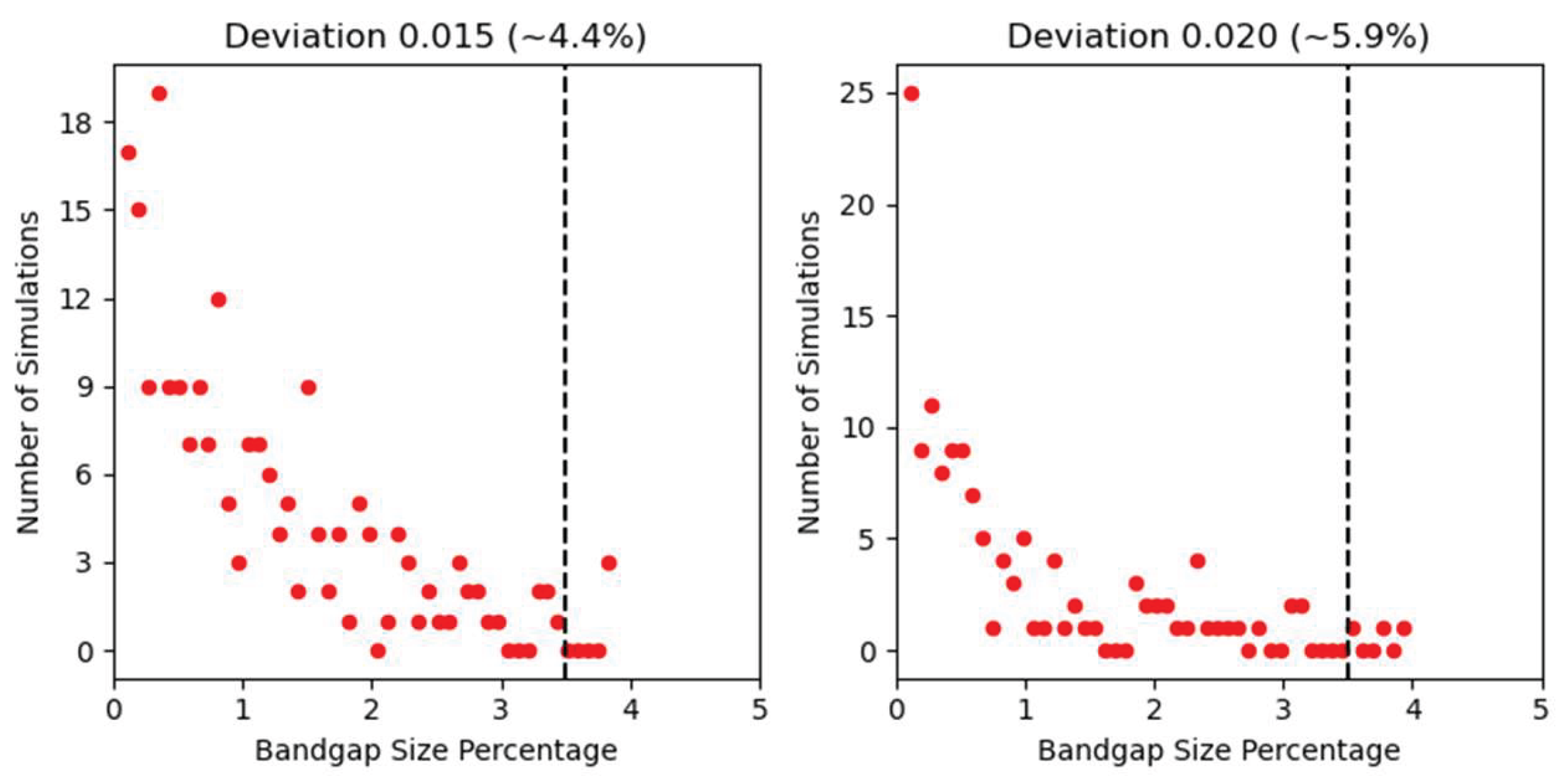
Histograms plotting the occurrence frequency of bandgap percentage from simulations for the standard deviation values σ/a = 0.015 (left) and 0.020 (right); these are the two data sets without an applicable Gaussian line-fit. For additional scaling clarity, the “zero bins” have been excluded from these plots. The black dotted line indicates the bandgap percentage of the original ordered cells, 3.5%.
Figure A1.
Histograms plotting the occurrence frequency of bandgap percentage from simulations for the standard deviation values σ/a = 0.015 (left) and 0.020 (right); these are the two data sets without an applicable Gaussian line-fit. For additional scaling clarity, the “zero bins” have been excluded from these plots. The black dotted line indicates the bandgap percentage of the original ordered cells, 3.5%.
Appendix B
Installation of MEEP
Ubuntu version 22.04 was used for this installation of MEEP (v1.29.0), although most Linux systems should be useable. Anaconda, a package manager for Python packages, is required. For an x86 system, the relevant download file can be found on https://www.anaconda.com/download/success. Installation of Conda is done through a terminal window with the following command:
bash <conda-installer-name>-latest-Linux-x86_64.sh
A Conda environment for MEEP is then created and MEEP is downloaded:
conda create -n mp -c conda-forge pymeep pymeep-extras
To activate this environment:
To activate this environment:
conda activate mp
This activation may be required to be done through the Anaconda Console. MEEP can then be imported as normal to a python IDE launched through Anaconda. MPB is included in the installation and can be imported by:
from meep import mpb
The OpenMPI version used for this project was the public download of OpenMPI from https: //www.open-mpi.org/software/ompi/v5.0/ and was built from the .tar.bz2 file, rather than the officially supported Parallel MEEP’s OpenMPI implementation. To build, a temporary build directory and installation directory were created on the Desktop (although this could be done elsewhere):
export BUILD_DIR = $HOME/Desktop/MPI_Build
mkdir -p $BUILD_DIR
export INSTALL_DIR = $HOME/Desktop/MPI_Install
mkdir -p $INSTALL_DIR
mkdir -p $BUILD_DIR
export INSTALL_DIR = $HOME/Desktop/MPI_Install
mkdir -p $INSTALL_DIR
The .tar.bz2 file was downloaded and placed in the build directory. The current version was 5.0.8, which will be used here. The following commands were used to build OpenMPI:
cd $BUILD_DIR
tar xf openmpi-5.0.8.tar.bz2
cd openmpi-5.0.8
mkdir build
cd build/
../configure --prefix=$INSTALL_DIR/ompi
make -j $(nproc)
make install
tar xf openmpi-5.0.8.tar.bz2
cd openmpi-5.0.8
mkdir build
cd build/
../configure --prefix=$INSTALL_DIR/ompi
make -j $(nproc)
make install
This had the unintended side effect of allowing the MPB simulations to run on only one physical core (normally, MPB uses all available cores). For an 8-core system, each core could be assigned its own simulation, for 8 total simulations at once. For the three-dimensional randomisation code, MPB using all 8 cores for one simulation took approximately 30 minutes on the Ryzen 7 CPU used. If each core was assigned its own simulation, it would take approximately 90 minutes, but produce 8 independent results, a notable speed increase. To run, navigate to the folder with the filele then:
where the 8 is the number of cores. An error will appear if more cores than the system physically has are assigned.
conda activate mp
$HOME/Desktop/MPI_Install/ompi/bin/mpirun -np 8 python <python_filename>.py
$HOME/Desktop/MPI_Install/ompi/bin/mpirun -np 8 python <python_filename>.py
There was an error discovered where attempting to loop the execution of the bandgap solver in python would result in non-random behaviour for the random three-dimensional system for both regular and MPI executions of the python file. This was solved by looping through the terminal instead, over a range of 1 to some number (shown as 24 below):
for i in {1..24}; \
do $HOME/Desktop/MPI_Install/ompi/bin/mpirun -np 8 python <python_filename>.py “$i”; \
done
do $HOME/Desktop/MPI_Install/ompi/bin/mpirun -np 8 python <python_filename>.py “$i”; \
done
References
- Joannopoulos, J.D.; Johnson, S.G.; Winn, J.N.; Meade, R.D. Photonic Crystals Molding the Flow of Light, 2nd ed.; Princeton University Press: Princeton, 2008; ISBN 978-0-691-12456-8. [Google Scholar]
- Yablonovitch, E. Inhibited Spontaneous Emission in Solid-State Physics and Electronics. Phys Rev Lett 1987, 58. [Google Scholar] [CrossRef]
- Russell, P.S.J. Photonic Band Gaps. Physics World 1992, 5, 37. [Google Scholar] [CrossRef]
- Chistyakov, V.A.; Sidorenko, M.S.; Sayanskiy, A.D.; Rybin, M. V. Density of Photonic States in Aperiodic Structures. Phys Rev B 2023, 107, 014205. [Google Scholar] [CrossRef]
- Cregan, R.F.; Mangan, B.J.; Knight, J.C.; Birks, T.A.; Russell, P.S.J.; Roberts, P.J.; Allan, D.C. Single-Mode Photonic Band Gap Guidance of Light in Air. Science (1979) 1999, 285. [Google Scholar] [CrossRef]
- Alexander, K.; Bahgat, A.; Benyamini, A.; Black, D.; Bonneau, D.; Burgos, S.; Burridge, B.; Campbell, G.; Catalano, G.; Ceballos, A.; et al. A Manufacturable Platform for Photonic Quantum Computing. Nature 2025 641:8064 2025, 641, 876–883. [Google Scholar] [CrossRef]
- Parker, G.; Charlton, M. Photonic Crystals. Physics World 2000, 13, 29. [Google Scholar] [CrossRef]
- López, C. Materials Aspects of Photonic Crystals. Advanced Materials 2003, 15. [Google Scholar] [CrossRef]
- Bermel, P.; Luo, C.; Zeng, L.; Kimerling, L.C.; Joannopoulos, J.D. Improving Thin-Film Crystalline Silicon Solar Cell Efficiencies with Photonic Crystals. Opt Express 2007, 15, 16986–17000. [Google Scholar] [CrossRef]
- Yeh, C. Applied Photonics; Academic Press: London, 2012; ISBN 0080499260,9780080499260. [Google Scholar]
- Russell, P.S.J. Photonic-Crystal Fibers. Journal of Lightwave Technology 2006, 24. [Google Scholar] [CrossRef]
- Russell, P.S.J.; Knight, J.C.; Birks, T.A.; Mangan, B.J.; Wadsworth, W.J. Recent Progress in Photonic Crystal Fibres. In Proceedings of the Conference on Optical Fiber Communication, Technical Digest Series, 2000; Vol. 3. [Google Scholar]
- Joannopoulos, J.D.; Villeneuve, P.R.; Fan, S. Photonic Crystals: Putting a New Twist on Light. Nature 1997, 386, 143–149. [Google Scholar] [CrossRef]
- Hsia, H.; Tsai, C.H.; Ting, K.C.; Kuo, F.W.; Lin, C.C.; Wang, C.T.; Hou, S.Y.; Chiou, W.C.; Yu, D.C.H. Heterogeneous Integration of a Compact Universal Photonic Engine for Silicon Photonics Applications in HPC. In Proceedings of the Proceedings - Electronic Components and Technology Conference, 2021; Vol. 2021-June. [Google Scholar]
- Mandal, M.; De, P.; Lakshan, S.; Sarfaraj, M.N.; Hazra, S.; Dey, A.; Mukhopadhyay, S. A Review of Electro-Optic, Semiconductor Optical Amplifier and Photonic Crystal-Based Optical Switches for Application in Quantum Computing. Journal of Optics (India) 2023, 52, 603–611. [Google Scholar] [CrossRef]
- Vukusic, P.; Sambles, J.R. Photonic Structures in Biology. Nature 2003, 424, 852–855. [Google Scholar] [CrossRef] [PubMed]
- Middleton, R.; Tunstad, S.A.; Knapp, A.; Winters, S.; McCallum, S.; Whitney, H. Self-Assembled, Disordered Structural Color from Fruit Wax Bloom. Sci Adv 2024, 10, 4219. [Google Scholar] [CrossRef] [PubMed]
- Saba, M.; Thiel, M.; Turner, M.D.; Hyde, S.T.; Gu, M.; Grosse-Brauckmann, K.; Neshev, D.N.; Mecke, K.; Schröder-Turk, G.E. Circular Dichroism in Biological Photonic Crystals and Cubic Chiral Nets. Phys Rev Lett 2011, 106. [Google Scholar] [CrossRef]
- Noh, J.; Benalcazar, W.A.; Huang, S.; Collins, M.J.; Chen, K.P.; Hughes, T.L.; Rechtsman, M.C. Topological Protection of Photonic Mid-Gap Defect Modes. Nat Photonics 2018, 12, 408–415. [Google Scholar] [CrossRef]
- Yuan, T.; Feng, T.; Xu, Y.I. Manipulation of Transmission by Engineered Disorder in One-Dimensional Photonic Crystals. Optics Express 2019, Vol. 27(Issue 5 27), 6483–6494. [Google Scholar] [CrossRef]
- Rothammer, M.; Zollfrank, C.; Busch, K.; Freymann, G. von Tailored Disorder in Photonics: Learning from Nature. Adv Opt Mater 2021, 9, 2100787. [Google Scholar] [CrossRef]
- Yu, S.; Qiu, C.W.; Chong, Y.; Torquato, S.; Park, N. Engineered Disorder in Photonics. Nat Rev Mater 2021, 6, 226–243. [Google Scholar] [CrossRef]
- Wiersma, D.S. Disordered Photonics. Nat Photonics 2013, 7, 188–196. [Google Scholar] [CrossRef]
- Segev, M.; Silberberg, Y.; Christodoulides, D.N. Anderson Localization of Light. Nat Photonics 2013, 7, 197–204. [Google Scholar] [CrossRef]
- An, T.; Jiang, X.; Gao, F.; Schäfer, C.; Qiu, J.; Shi, N.; Song, X.; Zhang, M.; Finlayson, C.E.; Zheng, X.; et al. Strain to Shine: Stretching-Induced Three-Dimensional Symmetries in Nanoparticle-Assembled Photonic Crystals. Nat Commun 2024, 15. [Google Scholar] [CrossRef]
- Dolan, J.A.; Wilts, B.D.; Vignolini, S.; Baumberg, J.J.; Steiner, U.; Wilkinson, T.D. Optical Properties of Gyroid Structured Materials: From Photonic Crystals to Metamaterials. Adv Opt Mater 2015, 3, 12–32. [Google Scholar] [CrossRef]
- Piechulla, P.M.; Muehlenbein, L.; Wehrspohn, R.B.; Nanz, S.; Abass, A.; Rockstuhl, C.; Sprafke, A. Fabrication of Nearly-Hyperuniform Substrates by Tailored Disorder for Photonic Applications. Adv Opt Mater 2018, 6, 1701272. [Google Scholar] [CrossRef]
- Oskooi, A.F.; Roundy, D.; Ibanescu, M.; Bermel, P.; Joannopoulos, J.D.; Johnson, S.G. Meep: A Flexible Free-Software Package for Electromagnetic Simulations by the FDTD Method. Comput Phys Commun 2010, 181, 687–702. [Google Scholar] [CrossRef]
- Johnson, S.G.; Joannopoulos, J.D.; Meade, R.D.; Rappe, A.M.; Brommer, K.D.; Alerhand, O.L. Block-Iterative Frequency-Domain Methods for Maxwell’s Equations in a Planewave Basis. Optics Express 8(Issue 3 8), 173-190. [CrossRef] [PubMed]
- Koenderink, A.F.; Lagendijk, A.; Vos, W.L. Optical Extinction Due to Intrinsic Structural Variations of Photonic Crystals. Phys Rev B Condens Matter Mater Phys 2005, 72, 153102. [Google Scholar] [CrossRef]
- MEEP Documentation https://Meep.Readthedocs.Io. Accessed. (accessed on 18 November 2025).
- Yee, K.S. Numerical Solution of Initial Boundary Value Problems Involving Maxwell’s Equations in Isotropic Media. IEEE Trans Antennas Propag 1966, 14, 302–307. [Google Scholar] [CrossRef]
- MPB Documentation https://Mpb.Readthedocs.Io/En/Latest/Python_Tutorial/. Accessed. (accessed on 9 December 2025).
- Tétreault, N.; Míguez, H.; Ozin, G. Silicon Inverse Opal—A Platform for Photonic Bandgap Research. Adv. Mater. 2004, 16, 1471–1476. [Google Scholar] [CrossRef]
- Zhao, Q.; Finlayson, C.; Snoswell, D.; et al. Large-scale ordering of nanoparticles using viscoelastic shear processing. Nat Commun 2016, 7, 11661. [Google Scholar] [CrossRef]
Figure 1.
(a) unit cell schematic of a 3D photonic crystal fcc-lattice of spheres. The lattice parameter , the sphere radius , and the geometric interrelation of and are as indicated. The relation shown r/a is the largest radius before the spheres intersect. This lattice may be of high-index (dielectric) spheres in a medium of low-index (e.g., air), or vice-versa to give an “inverse opal” structure. (b) The corresponding k-space diagram of the fcc-lattice.
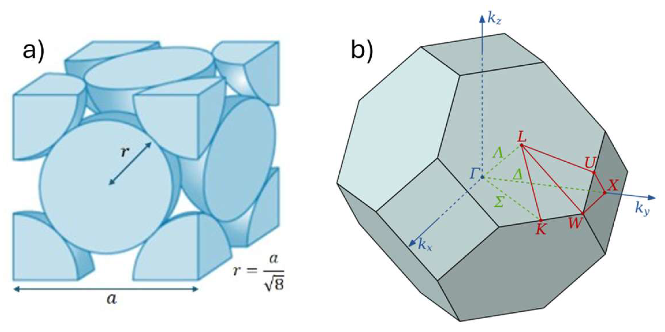
Figure 2.
Dispersion relation diagram showing the bands of an “Inverse Opal” Silicon lattice with a bandgap of 3.5% between 0.697 c/a and 0.722 c/a. The background material has dielectric constant ε = 13 and the spheres ε = 1. (a) Bands of the unit cell. The sphere radius is r/a = 0.34. (b) Bands of a 2 x 2 x 2 supercell lattice with uniform sphere radii r/a = 0.34.
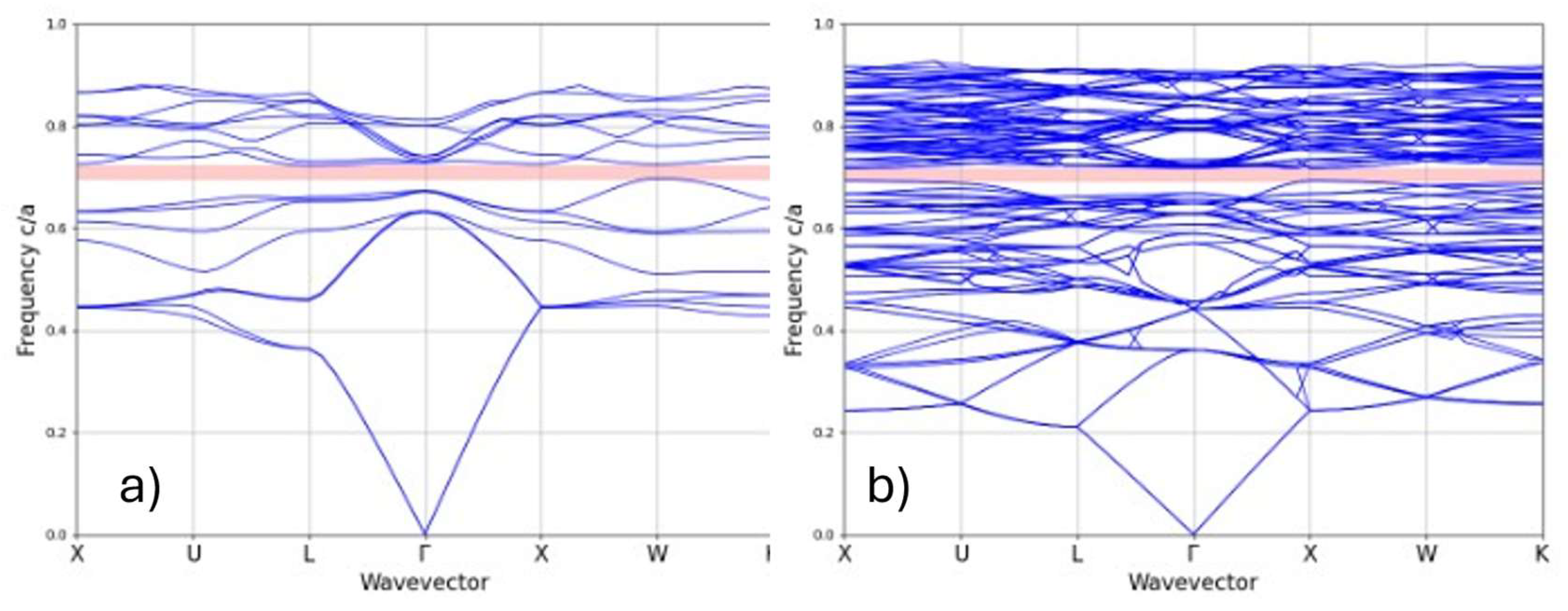
Figure 3.
Occurrence of all radius values for each standard deviation (σ) studied plotted into 50 discreet intervals. Each simulation produced eight radii values for eight spheres, for a grand total of 8x radii values multiplied by the number of simulations.
Figure 3.
Occurrence of all radius values for each standard deviation (σ) studied plotted into 50 discreet intervals. Each simulation produced eight radii values for eight spheres, for a grand total of 8x radii values multiplied by the number of simulations.
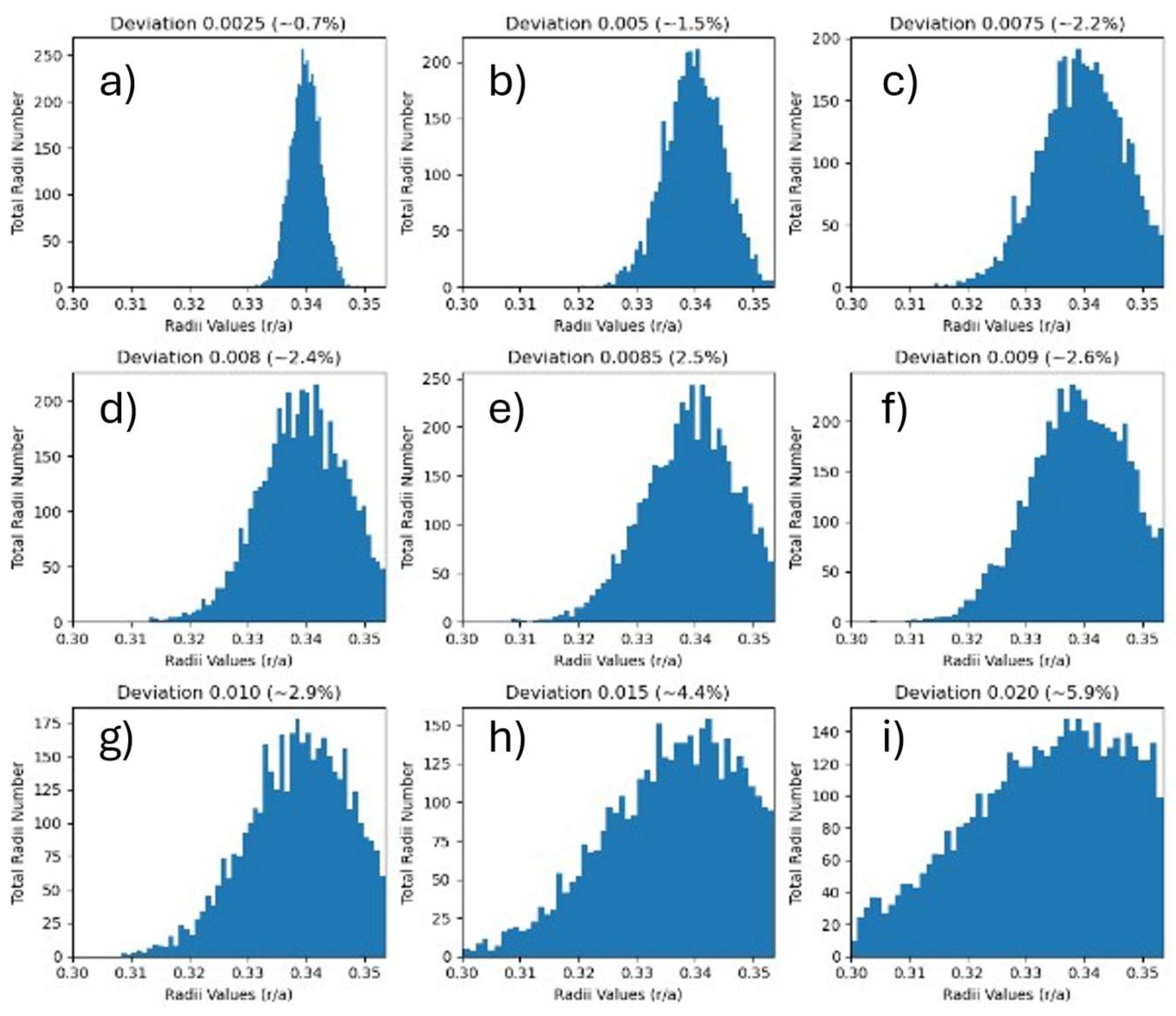
Figure 4.
Histograms plotting the occurrence frequency of bandgap percentage, for each standard deviation value studied, as indicated in (a) through (i). The black dotted line indicates the bandgap percentage of the original ordered cells, 3.5%. The blue line is a Gaussian fit to the data points, with the zero bins being excluded from the fit. Plots (h) and (i) do not have fits, as there are too few non-zero generated points to reliably infer a Gaussian distribution.
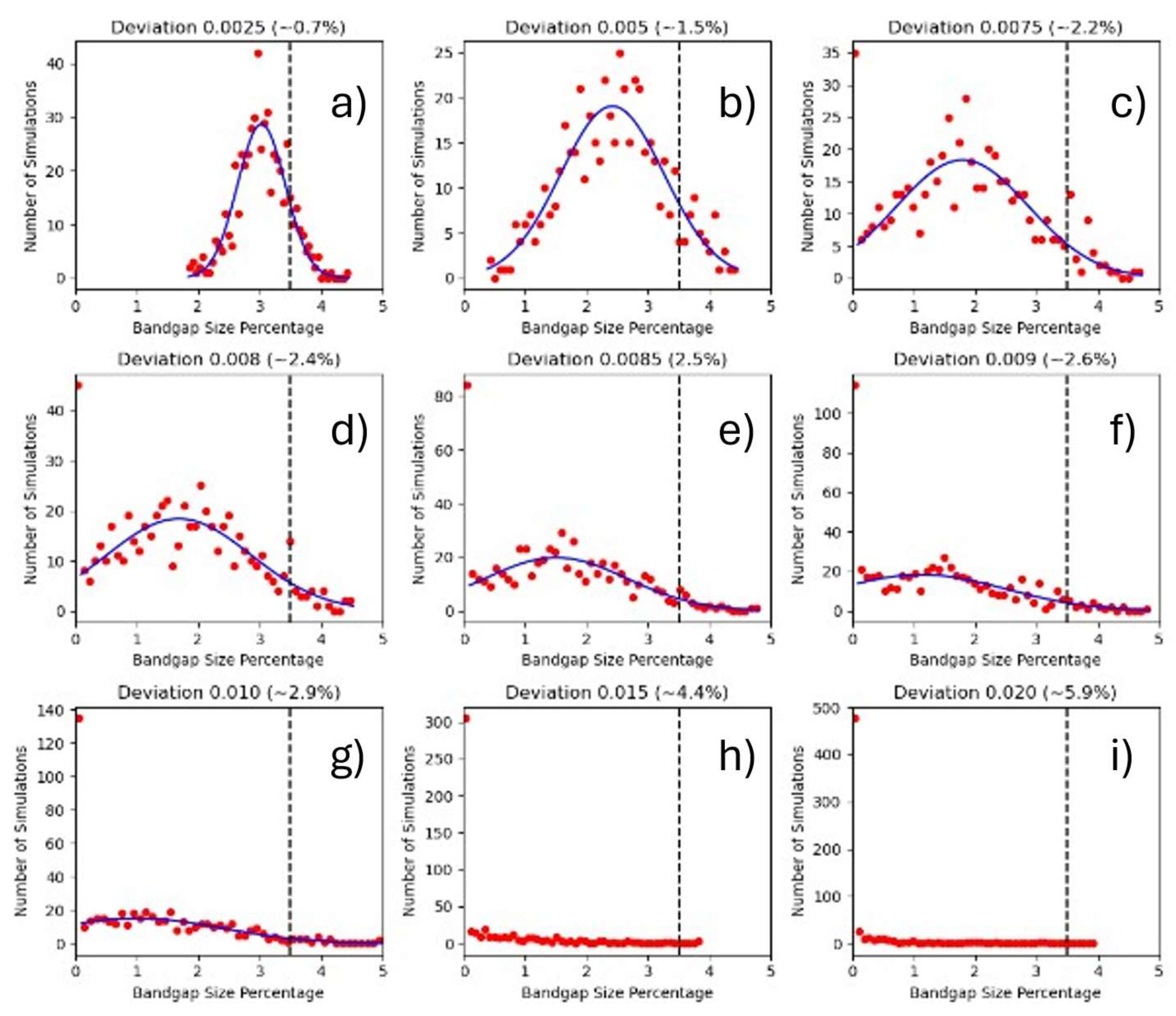
Figure 5.
Extracted parameters of the Gaussian fitting for the simulation data sets plotted versus radii standard deviation (σ/a); in a), mean bandgap as a percentage of normalized frequency range (Μ) and associated standard deviation (Σ), in b) the fraction of simulations with bandgap magnitude greater than the 3.5% baseline (Λ), and in c) the fraction of simulations with non-zero bandgap (Ω). In a), notional Μ and Σ values for the σ/a = 0 case are included (circles) to elucidate trends. In b), an indicative exponential fit trendline is displayed, with a 1/e decay constant of 0.0072. In c), a sigmoidal fit is displayed (log-log plot), as per the function shown in the inset, with the values of y0 and y1 set at 1 and -1 respectively, and the best-fitted values being = 0.0140 and = 0.0031.
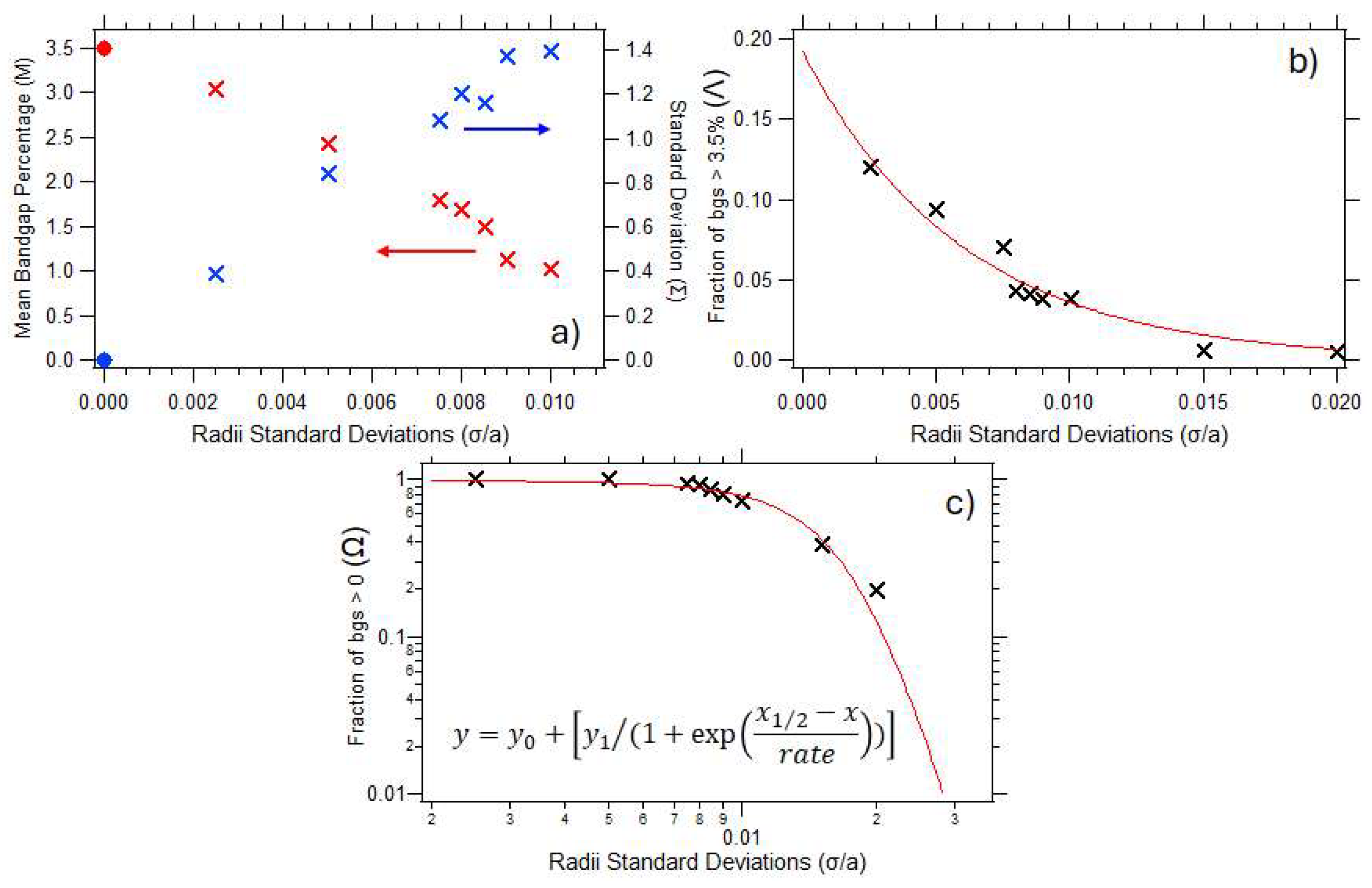
Figure 6.
Dispersion relation diagrams illustrating the bands for representative simulation outputs from inverse opal Silicon 2 x 2 x 2 supercell lattices. Bandgap magnitudes are, (a) zero, (b) narrow (1-3% fractional range), (c) comparable to the original in the 3-4% fractional range, and (d larger than the original in the 4-5% fractional range. The corresponding values of σ/a were 0.020, 0.005, 0.005, and 0.010 from a) to d) respectively.
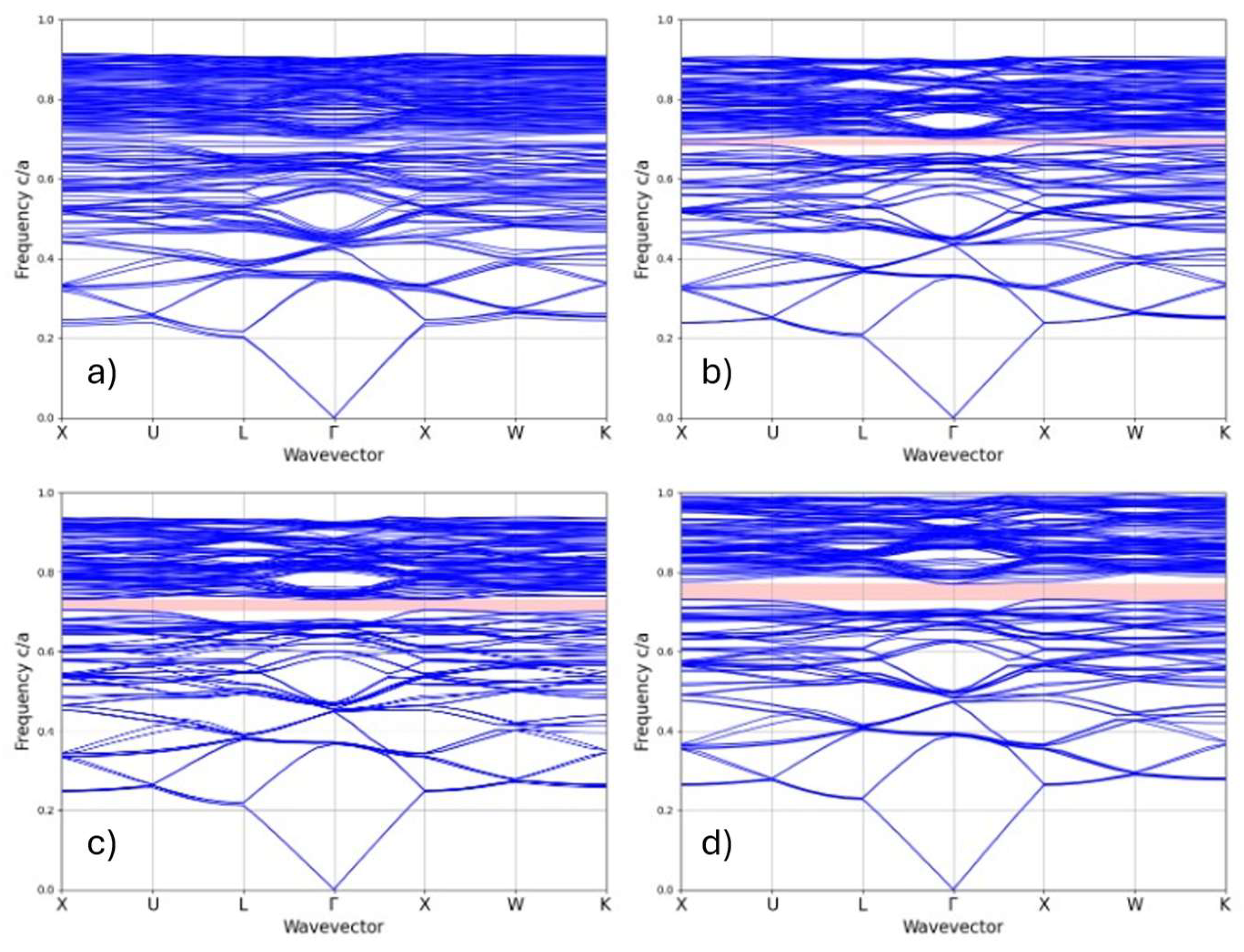

Table 1.
Gives the range of radii standard deviations used in simulations (σ/a), also expressed as a percentage of the mean radius (σ/μ). Extracted parameters of the Gaussian fitting for the simulation data sets; mean bandgap in percentage of frequency range (Μ), with standard deviation (Σ). Ω and Λ are the cumulative fractions of individual simulations with finite non-zero bandgaps and bandgaps greater than the baseline ordered structures, respectively. The data sets for σ/a = 0.015 and σ/a = 0.020 do not have a valid Gaussian fit so parameters Μ and Σ are left empty.
| Radii Standard Deviations | Bandgap Values | ||||
|---|---|---|---|---|---|
| Standard Deviation σ /a | Percent of the Mean σ /m | Mean Bandgap Percentage (M) | Standard Deviation (S) | Fraction of Bandgaps > 0 (Ω) | Fraction of Bandgaps ≥ 3.5% (Λ) |
| 0.020 | ~5.9% | 0.197±0.033 | 0.005±0.0002 | ||
| 0.015 | ~4.4% | 0.385±0.028 | 0.006±0.0003 | ||
| 0.010 | ~2.9% | 1.01±0.04 | 1.39±0.06 | 0.736±0.012 | 0.038±0.0017 |
| 0.009 | ~2.6% | 1.12±0.05 | 1.37±0.06 | 0.802±0.008 | 0.038±0.0016 |
| 0.0085 | 2.5% | 1.50±0.06 | 1.16±0.05 | 0.860±0.006 | 0.041±0.0017 |
| 0.008 | ~2.4% | 1.69±0.05 | 1.20±0.06 | 0.925±0.004 | 0.043±0.0018 |
| 0.0075 | ~2.2% | 1.80±0.08 | 1.08±0.05 | 0.934±0.003 | 0.070±0.0030 |
| 0.005 | ~1.5% | 2.42±0.11 | 0.84±0.04 | >0.999 | 0.094±0.0043 |
| 0.0025 | ~0.7% | 3.03±0.13 | 0.39±0.02 | >0.999 | 0.120±0.0051 |
Disclaimer/Publisher’s Note: The statements, opinions and data contained in all publications are solely those of the individual author(s) and contributor(s) and not of MDPI and/or the editor(s). MDPI and/or the editor(s) disclaim responsibility for any injury to people or property resulting from any ideas, methods, instructions or products referred to in the content. |
© 2026 by the authors. Licensee MDPI, Basel, Switzerland. This article is an open access article distributed under the terms and conditions of the Creative Commons Attribution (CC BY) license.
Copyright: This open access article is published under a Creative Commons CC BY 4.0 license, which permit the free download, distribution, and reuse, provided that the author and preprint are cited in any reuse.


