
Submitted:
26 January 2026
Posted:
27 January 2026
You are already at the latest version
Abstract
Recent laboratory experiments in an intermediate-scale Hele-Shaw cell, designed to emulate a coarse sand aquifer, demonstrate that calcite precipitation induced by mixing leads to the formation of a self-organized, heterogeneous porous medium. This medium is characterized by elongated carbonate structures and internal preferential flow channels aligned with the main flow direction. The resulting transport behavior exhibits strong anomalous features, as evidenced by breakthrough curves showing earlier solute arrival, a distinct double peak, and pronounced tailing. In this article, we investigate the relationship between the self-organized heterogeneous structure of the porous medium formed through mixing-induced precipitation and its impact on solute transport. To achieve this, we analyze the spatial variability of hydraulic conductivity by implementing different permeability scenarios in a random walk particle tracking model. These scenarios, derived from image analysis of the precipitated structures, range from simple representations to increasingly complex configurations. Our results highlight the importance of capturing two key features to effectively describe solute transport. First, delineating the total precipitated area is crucial for accurately representing flow diversion caused by permeability reduction, which explains the emergence of the double peak in solute concentrations. However, fully capturing both the double peak transition and tailing requires representing the internal structure of the high-precipitation zones within the precipitated area, as these characterize internal preferential flow channels.
Keywords:
groundwater flow
; solute transport
; heterogeneity
; mixing-induced precipitation
; MODPATH-RW
1. Introduction
Mineral precipitation is a fundamental geochemical process in porous media that can significantly alter the hydraulic and transport properties of aquifers [1,2,3]. This phenomenon typically occurs when waters with different chemical signatures mix, creating supersaturation conditions that promote the formation of new minerals in the porous matrix [4,5]. Over time, sustained precipitation can progressively clog the pores of the medium, reducing the effective porosity and permeability of the system, which, in turn, influences groundwater flow and solute transport [6,7,8]. Among the various types of mineral precipitation, carbonate precipitation has gained increasing attention due to its significant role in subsurface engineering applications [9,10,11], particularly in environments where calcium- and carbonate-rich waters interact [12]. Recent advancements have focused on controlled precipitation techniques, such as microbially induced calcium carbonate precipitation (MICP) [13,14,15] and enzymatic methods [16,17,18]. These techniques enable targeted mineral formation in specific subsurface environments, offering precise control over mineral deposition and its effects on permeability [19]. These precipitation techniques have found widespread applications across various disciplines [20]. For instance, in geological carbon sequestration (GCS), carbonate precipitation is intentionally induced to seal preferential flow paths in low-permeability cap rocks, reducing the risk of CO2 leakage [21,22,23]. Similarly, in enhanced oil recovery (EOR), MICP has proven successful in modifying rock permeability by plugging high-permeability flow channels, thereby enhancing sweep efficiency and optimizing hydrocarbon extraction [24,25,26]. However, the efficiency of these techniques is strongly influenced by the spatial heterogeneity that mineral precipitation introduces within the porous medium [5,27,28]. This heterogeneity [29,30], significantly affects the spatial variability in hydraulic conductivity, which in turn impacts solute transport. Therefore, understanding the relationship between the heterogeneous structure of the porous medium formed through mixing-induced precipitation and its impact on solute transport is crucial for improving the use of precipitation-based techniques in environmental and engineering applications.
Prior research has identified two distinct categories of mineral precipitation mode, preferential precipitation, and uniform precipitation [31,32,33]. In the preferential precipitation mode, the solid phase tends to form scattered crystals on the rock-fluid interface [34,35], forming a heterogeneous precipitation texture that evolve across multiple spatial and temporal scales [5,27], whereas the uniform precipitation mode results in a uniform coating of precipitate [28]. Three predominant factors influence these mineral precipitation modes: solute mixing [5], mineral nucleation [28], and the relative timescale of reaction kinetics compared to ion transport [36].
Solute mixing plays a critical role in influencing the spatiotemporal evolution of reaction products [37,38,39]. This mixing affects the spatial distribution and concentration of dissolved ions, which, in turn, influences the precipitation process. Spatiotemporal patterns in the development of CaCO3 deposits have been reported, including small isolated deposits on the surface of the porous medium grains, elongated structures following the main flow direction, and homogeneous precipitates along the flow front. Mineral nucleation, however, remains a complex phenomenon involving various physical processes such as fluid flow, species transport, interfacial processes, and geochemical reactions [33,40,41]. The nucleation rate plays a crucial role in determining the density and distribution of newly formed crystals [28]. A high nucleation rate leads to a more uniform distribution of the solid phase, while a lower nucleation rate results in fewer, larger crystals that grow rapidly, promoting mineral heterogeneity and causing a more pronounced reduction in hydraulic conductivity. Alongside nucleation, the relative timescale of reaction kinetics compared to ion transport is vital in shaping mineral precipitation [36,42,43]. When reaction rates are slow relative to transport, dissolved ion concentrations remain relatively uniform, fostering consistent mineral growth. However, when reaction kinetics surpass ion replenishment, concentration gradients develop, leading to localized precipitation.
The spatial variability of mineral precipitation, resulting from these factors, drives non-uniform changes in local reaction rates that modify the internal structure of the porous medium [29,30]. This, in turn, increases permeability variations at multiple scales, promoting the formation of preferential flow paths [44,45]. Experimental studies focused on sealing fractured rocks have demonstrated that mineral precipitation generates self-organizing flow channels within the fracture network [34,46]. As these areas fill, the flow is progressively redirected to regions where no precipitation occurs, forming new flow paths [34], with tortuous and braided pathways emerging within the fracture [46]. The heterogeneity caused by preferential precipitation in porous media has profound implications for solute transport. The irregular distribution of precipitates and channeling significantly modifies flow velocities and dispersive properties, leading to deviations from classical Fickian behavior. This non-Fickian transport manifests as anomalous breakthrough curves, which traditional models fail to accurately capture [47,48]. The challenge in modeling these systems lies in the difficulty of characterizing the spatial variability of permeability caused by freshly formed precipitates. Successfully addressing this challenge requires determining the appropriate level of complexity needed to accurately represent anomalous transport and identifying the key features that must be incorporated into numerical models.
This study investigates the relationship between precipitation-induced heterogeneities and solute transport by analyzing dominant precipitation patterns and their impact on breakthrough concentrations. Conservative tracer tests were conducted on an experimental aquifer before and after mixing-induced calcite precipitation to assess how heterogeneities at different scales evolve with time and impact solute transport behavior. These experiments build on previous experimental findings [48], which identified unusual breakthrough curves with dual peaks and extended tails, directly linked to precipitation-induced structural heterogeneity. To address these phenomena, this study presents the interpretation of the experiment through a solute transport model that simulates anomalous transport behavior resulting from mineral precipitation using a novel method to characterize the spatial variability of permeability determine from image analysis. In this context, this work aims to: (i) evaluate how to characterize the heterogeneity in order to reproduce the anomalous solute transport behavior after mineral precipitation, (ii) understand the level of complexity required to accurately reproduce solute transport in heterogeneous systems, and (iii) assess the key features of heterogeneity that must be represented in numerical models to correctly reproduce solute transport. To achieve these goals, this study introduces a numerical model that simulates solute transport in porous media affected by mineral precipitation. The model incorporates detailed representations of the evolving spatial heterogeneity resulting from the precipitation process. By leveraging laboratory-derived data on permeability fields influenced by calcite precipitation, this research offers a unique perspective on how varying levels of heterogeneity—driven by both the amount and distribution of precipitate affect solute transport. The methodology includes a comparative analysis between homogeneous and heterogeneous models, where the latter is defined by multiple permeability zones based on varying image intensities of the precipitation. This approach allows for a deeper understanding of the relationship between the distribution of the precipitated mineral and its influence on solute transport, while also highlighting the critical role of spatial variability in accurately predicting solute transport. The novelty of this approach lies in the ability to replicate the anomalous transport behavior observed in real-world systems that are affected by transient precipitation processes. Furthermore, this study provides valuable insights into the implications of incorporating heterogeneous permeability fields induced by precipitation into transport models, which can be applied to both field studies and laboratory experiments. In particular, the findings have direct relevance for applications in environmental engineering, such as carbon sequestration enhanced oil recovery (EOR), where mineral precipitation is often used to enhance solute retention and mobility.
The structure of this article is as follows. The Experimental Overview section summarizes previous experiments conducted on Mixing-Driven Precipitation (MDP) and tracer tests, including the setup, procedure, and main findings. The Methods section describes the methodology implemented to create the composite permeability fields, presents the flow and transport model, and explains the model calibration. The Results and Discussion section presents the main findings obtained from the dual- and triple-permeability composite field models. Finally, the Conclusions section summarizes the key insights, emphasizing the importance of accurately characterizing the heterogeneity caused by mineral precipitation to effectively represent the resulting anomalous solute transport.
2. Experimental Overview
A laboratory experiment was conducted by Guido González-Subiabre and Fernàndez-Garcia [48], to evaluate the impact of mineral precipitation induced by mixing on solute transport, consisting of three main stages (Figure 1a). First, an initial conservative tracer test (T1) was performed to establish the systems initial transport conditions through a breakthrough curve (BTC). This was followed by the Mixing-Driven precipitation (MDP) experiment, during which synthetic solutions of CaCl2 () and Na2CO3 () were simultaneously and uniformly injected in parallel, each through half of the inlet face of the tank, to form the calcite layer. This configuration induces a mixing zone that extends along the centerline of the tank as shown in Figure 1b. The solutions were selected based on previous experimental research [7,49,50]. Finally, a second conservative tracer test (T2) was conducted to capture changes in the BTC resulting from the freshly formed calcite after the MDP stage. A detailed description of the experimental procedure, the setup and the results is provided by Guido González-Subiabre and Fernàndez-Garcia [48]. A two-dimensional horizontal tank made of plexiglass, designed to replicate a coarse sand granular confined aquifer, was used to perform the Mixing-Driven Calcite Precipitation (MDP) experiment and companion conservative tracer tests (Figure 1b). The tank was homogeneously wet-packed with spherical glass beads (d = 2 mm) and initially filled with deionized water (Milli-Q). The synthetic aquifer was designed to provide uniform flow conditions, featuring eight inlet and outlet ports spaced 2 cm apart. To monitor the evolution of the freshly precipitated calcite, image analysis was employed. The experimental setup was placed in a darkroom to minimize external light interference, while a 1550 Lm, 20 W Downlight LED positioned above the tank served as the light source for visualization. The intensity of the reflected light was then used to track the development of the precipitate over time. Images were captured every 30 seconds using a Nikon D7100 camera paired with a Tamron SP AF17-50mm F/2.8 XR Di II LD Aspherical (IF) Model A16 lens. For the tracer tests, a fluorescein solution with a uniform inlet concentration of c0 = 3 mg/L was used. The concentrations at the outlet were measured with an Albillia FL24 fluorometer, which provided an integrated breakthrough curve for the entire system. Continuous monitoring with the fluorometer was conducted, taking measurements every second. Precipitation and tracer test experiments were conducted under advection-dominated transport conditions, supported by a grain Péclet number of Pe = 523. A prescribed flow boundary was established at the system entry with a total inflow rate of Q= 1.78 , evenly distributed using 8 inlet ports. A constant head boundary condition was imposed (0.9 m above the tank elevation) at the tank outlet. The initial hydraulic conductivity () and porosity () of the system were both experimentally estimated, with = 145.4 m/day and = 0.34. For the experimental properties of the synthetic aquifer used in the experiment, consult Table 1. The results obtained in the experiment are shown in Figure 1(c). This finding indicated that after the MDP experiment, a symmetric, bell-shaped precipitation front was formed with a self-organized, heterogeneous pattern. This pattern was characterized by internal elongated carbonate structures that created preferential flow paths. Breakthrough curves revealed a shift in solute transport behavior from a classical Fickian-like distribution to a non-Fickian anomalous distribution, exhibiting a double-peak curve with pronounced tailing. Although the origin of this phenomenon is not fully understood, it is hypothesized to involve channeling and back-diffusion in low-permeability zones. Guido González-Subiabre and Fernàndez-Garcia [48] observed that precipitation-induced heterogeneity affects solute transport, yet the underlying mechanisms remain unclear. Simulating such heterogeneity in transport models is challenging due to the difficulty in capturing the evolving pore structure and permeability across multiple scales. This article provides insights to effectively represent mineral-induced heterogeneity in transport models. To understand the observed anomalies, we focus on modeling the heterogeneity caused by mineral precipitation. This is accomplished by processing the steady-state calcite precipitation image using a novel method to generate permeability fields that reflect the complexity of the induced heterogeneity. Different degrees of complexity are examined. The image processing technique, based on Schuszter et al. [51], assumes that the precipitate amount is proportional to the log of pixel intensity [51,52,53]. The generated permeability fields were designed to represent both the total area covered by the precipitate and regions with the highest concentration of precipitation, following a progressive approach from simple to complex representations. The breakthrough curve (BTC) obtained before mineral precipitation was used to determine the initial dispersivities ( and ), using a homogeneous permeability model characterized by a single hydraulic conductivity value ( = 145.4 m/day), representing the initial hydraulic conductivity measured for the system. For the BTC obtained after mineral precipitation, two different permeability distribution scenarios were considered: a dual-zone and a triple-zone composite permeability field.
3. Materials and Methods
3.1. Construction of Composite Permeability Fields
The calcite image obtained after mineral precipitation was used to generate different permeability scenarios, which were then implemented in the solute transport model. The image were processed using the OpenCV library in Python [55,56]. Self-organized, heterogeneous porous media, characterized by elongated carbonate structures and preferential flow channels, were represented using two permeability distribution scenarios: a dual and a triple composite permeability field.. First, the dual composite permeability fields were created by processing the image according to the steps outlined in [51], which assumes that the precipitate amount is proportional to the logarithm of the pixel intensity: (a) converting the image from raw format (NEF) to a 16-bit image (TIFF); (b) crop the image to focus on the precipitated zone which resulted in a region of interest (ROI) with resolution of 3975 x 3000 pixels, each pixel with an area of mm2; (c) transforming red, green and blue pixel intensity (, , into grayscale as
which results in a single-band representation of the image with ; (d) normalization of the grayscale pixel intensity to analyze image in the range [0,1] as
where is the grayscale light intensity distribution of a reference image representing a blank state obtained from the steady-state flow conditions prior to the MDP experiment, and , correspond respectively to the maximum and minimum grayscale intensities found in the image; (e) apply the logarithm of the normalized intensity ; f) create the histogram of the image (as shown in Figure 2a), to define the thresholds (Th) that will be used for the dual permeability fields; g) define four thresholds (Th) based on the percentile of the distribution of values. The percentiles were chosen within the range , which represents the precipitated area. The first threshold, = -2, represents the and was chosen through visual inspection to define the total precipitate area. From this value, three additional thresholds were defined to representing the internal structure of the high-precipitation zones within the precipitated area. = -0.6, which represents the and covers 15% of the total precipitated area; = -0.75, which represents the and covers 30% of the total precipitated area; and = -0.9, which represents the and covers 45% of the total precipitated area. A threshold above represents a very small area, which can be disregarded by the model. While values below would represent a very large area, losing the ability to differentiate it from the total precipitate area defined by .; h) binarizing the image based on each the selected thresholds as:
which results in four different images corresponding to the thresholds , , , and , where each pixel represents a value of 0 to represent the non-precipitated zone, or 1 to identify the precipitated zone; i) resize the binarized images (3000 x 3970) to the model size (200 x 265). Each pixel in the resized image represents the average of a 15x15 block from the original binarized images . If , the pixel is set to 1; otherwise, if , it is set to 0; j) create maps of the four binary images representing the areas affected by precipitation in blue (1) and the unaffected areas in red (0) (as shown in Figure 2b, e).
The triple permeability fields were created by progressively combining the four resized (200x265) binarized dual permeability fields. Initially, Field 1 and Field 2 were combined, resulting in the Field 1-2. This process continued for all possible combinations, creating six different combinations (Field 1-2, Field 1-3, Field 2-3, Field 4-3, Field 4-2, and Field 4-1). In our approach, each pixel in the resulting composite permeability field was calculated by summing the corresponding pixel values from the two original images at the same (x, y) position. In the resulting triple composite permeability fields, 0 represents a non-precipitated zone, 1 represents a precipitated zone, and 2 indicates the region of highest precipitation. These fields were then represented as maps, where red represents areas unaffected by precipitation, green indicates areas affected by precipitation, and blue highlights areas with the highest precipitation (as shown in Figure 3). The Field 1-2, Field 1-3, and Field 2-3 do not include the total real area covered by the precipitation, so they only represent different scenarios of the internal structure of the precipitated layer. In contrast, the Fields 4-3, Field 4-2, and Field 4-1, by considering Field 4, represent on one hand the total area covered by the precipitation and, on the other hand, three different scenarios to discretize the internal structures (Field 1, Field 2, and Field 3).

Table 2.
Pixel counts by field
| Field | Red pixels | Blue pixels | Green pixels |
|---|---|---|---|
| 1 | 51181 | 1819 | - |
| 2 | 48309 | 4691 | - |
| 3 | 44920 | 8080 | - |
| 4 | 34525 | 18475 | - |
| 2-1 | 48309 | 1819 | 2872 |
| 3-1 | 44920 | 1819 | 6261 |
| 3-2 | 44920 | 4691 | 3389 |
| 4-1 | 34525 | 1819 | 16656 |
| 4-2 | 34525 | 4691 | 13784 |
| 4-3 | 34525 | 8080 | 10395 |
3.2. Flow and Transport Model
The conservative breakthrough curves (BTCs) obtained before and after mineral precipitation were simulated through a flow and transport model. The flow model was developed under the assumption of steady-state conditions using MODFLOW-2005 [57], which solves the flow equation
where corresponds to the isotropic hydraulic conductivity, and h represents the piezometric head. The synthetic aquifer was simulated as a confined aquifer with a single layer, assuming steady-state condition. The dimensions of the flow model were 20 cm in width (W), 26.5 cm in length (L), and 1 cm in height (H). Flow and transport parameters implemented in the model are shown in Table 3. Cells of 1 mm in size were used, resulting in a grid with 200 rows and 265 columns. For the scenario representing the aquifer before mineral precipitation, a homogeneous model was applied using the initial hydraulic conductivity value measured in the experiment ( = 145.4 m/day). For the scenario representing the synthetic aquifer after mineral precipitation, a heterogeneous model was considered, utilizing either two or three hydraulic conductivities, depending on the model application scenario. For areas unaffected by mineral precipitation, the initial hydraulic conductivity value was used (). For the precipitated medium, the hydraulic conductivity values were determined through calibration. In the case of the dual-permeability model, only one hydraulic conductivity () was calibrated, while for the triple-permeability model, two hydraulic conductivities representing the calcite layer were calibrated ( and ), where represents the areas of higher precipitation within the layer, and therefore the area of lower hydraulic conductivity. In terms of the flow boundary conditions, a prescribed flow boundary was established at the system entry, with a total constant inflow rate (Q= 0.0154 m3/day), distributed across 8 ports (injection wells) at the entry, each represented by 5 cells, and for the system outlet a constant head boundary condition was imposed (0.9 m above the tank elevation). The solute transport model was developed using MODPATH-RW [58], an extension of the original MODPATH code [59] that is capable to simulate the advection-dispersion equation (ADE), which assumes Fickian dispersion at the local scale, using the Random Walk Particle Tracking (RWPT) method,
where is the medium porosity (dimensionless), c is the concentration of dissolved solute, is the specific discharge and is the hydrodynamic dispersion tensor, following the classic expression,
including both longitudinal () and transverse dispersivities (), the identity matrix () and the apparent molecular diffusion (), corrected by tortuosity. During the calibration of the homogeneous model (BTC obtained before mineral precipitation), both dispersivity coefficients ( and ) were adjusted. These values were then used to simulate the BTC obtained after calcite precipitation. The apparent molecular diffusion () was assigned a value of zero. The tracer test was simulated as a single specie, setting an injection time of 10 minutes in the eight injection wells at the entrance. The porosity () was set at a value of 0.34, which corresponds to the value obtained experimentally.
3.3. Model Calibration
Parameter calibration of each individual permeability composite models are evaluated by using two statistical indicators to select the best result for each scenario. The first is the RMSE (Root Mean Squared Error), defined by equation RMSE, and the second is the coefficient of determination R2, described in equation 7,
where n is the total number of observations/predictions, are the observed values, are the values predicted by the model, and is the mean of the observed values. The best result for each simulated scenario was selected considering on a high R2 and a low RMSE.
We consider that changes in local dispersivities due to mineral precipitation are negligible compared to the associated changes in permeability. Therefore, local dispersivities were held constant for all models and calibrated based on the initial tracer test conducted prior to the Mixing-Driven Precipitation (MDP) experiment. The process was manual and guided by these statistical metrics to ensure an accurate fit of the arrival time, peak concentration, and overall shape of the BTC. As shown in Figure 4(a), the model provides a good representation of the experimental BTC, with a coincidence in the arrival time, a peak value similar to that of the experiment, and an excellent fit, as demonstrated by the statistical indicators (R2= 0.9939, RMSE= 0.01946). Regarding the tailing, the simulated BTC exhibits a slight delay compared to the experimental BTC, as seen in greater detail in Figure 4(b). This behavior may be attributed either to reduced sensor accuracy at low concentrations or to anomalous transport processes, as noted by Levy and Berkowitz [60], which can lead to tailing even in homogeneous media. The resulting values are shown in Table 4.
To select the best model among all the different permeability scenarios simulated, the Akaike Information Criterion (AIC) was used, calculated by equation 8.
where n is the total number of observations (562), M is the number of parameters adjusted in the model (2 for the model with 2 hydraulic conductivities and 3 for the model with 3 hydraulic conductivities), and S is the sum of squared residuals (SSR), which is calculated as
The model with the lowest AIC, considering all scenarios, including both dual-permeability and triple-permeability models, is considered the best, as it indicates the best balance between model fit and complexity.
4. Results
4.1. Dual Composite Permeability Models
The non-Fickian transport observed in the experimental BTC, following mineral precipitation, was first evaluated using four dual composite permeability fields. The best fit of simulated BTCs for each scenario are shown in Figure 5, with the corresponding model parameters listed in Table 5. The results are presented in order of the total precipitated area covered by the permeability field, with the precipitated area shown in blue and the non-precipitated area shown in red. BTCs are shown with concentration values normalized (C/) and time expressed in pore volume (). In addition, they are also shown on a logarithmic scale.
We begin describing the result obtained for the Field 1 (Figure 5a), which has the smallest area considered for mineral precipitation. The simulated BTC does not capture the anomalous transport behavior observed in the experimental BTC (Figure 5b). Instead, it exhibits Fickian behavior, with a delayed arrival and a significantly higher peak (C/> 0.8). Regarding the tailing, the BTC does not account for the second peak observed in the experimental BTC and ends much earlier than the tail of the experimental BTC. It is interesting to highlight in this model that, although the BTC shows a Gaussian distribution, in Figure 5(c), it is evident that the low permeability zone results in an asymmetric distribution. To calibrate the BTC, the small area had to be assigned a very low hydraulic conductivity value ( = 8 m/day) for the precipitated area. resulting in the worst fit among the four fields (= 0.7063, RMSE = 0.1022, AIC = 998.66). Field 2 (Figure 5d) covers a larger precipitated area. Although the simulated BTC still exhibits Fickian behavior, it begins to show slight characteristics of anomalous transport (Figure 5e). The arrival time is now closer to that of the experimental BTC, and the peak value is lower than the values reached in Field 1 (< 0.8). The second peak, characteristic of the tailing, starts to appear subtly (Figure 5f). To calibrate the BTC, a slightly higher hydraulic conductivity ( = 17 m/day) was required, leading to a better fit compared to Field 1 (R2= 0.9180, RMSE= 0.0539, AIC= 279.52) . For Field 3 (Figure 5g), the simulated BTC no longer follows Fickian behavior, instead displaying characteristics of anomalous transport as reported in the experimental BTC (Figure 5h). Compared to Fields 1 and 2, the BTC better reproduces the arrival phase. However, the first peak remains poorly represented, with overestimated maximum values (C/< 0.8), while the second peak in the tailing is now clearly observed, with values close to those obtained from the experimental BTC (Figure 5i). Calibration indicates that the BTC obtained for this scenario achieves a better fit than the BTCs for Field 1 and Field 2 (R2 = 0.9595, RMSE= 0.0379, and AIC = -116.33). To calibrate the BTC to the considered area, a higher hydraulic conductivity value ( = 37 m/day) had to be assigned.
Finally, we present the simulated BTC for Field 4 (Figure 5j), which represents the entire area affected by precipitation. The simulated BTC exhibits non-Fickian behavior, more accurately capturing the anomalous transport observed in the experimental BTC (Figure 5k). Compared to the experimental BTC, it correctly represents the arrival, being the only one of the four fields to do so. Regarding the first peak, the model provides a good representation, slightly overestimating the values for the first peak (∼0.7). Similarly to Field 3, the BTC captures the second peak but overestimates its values (>0.1).
With respect to the tailing, as shown in Figure 5(k), the simulated BTC ends earlier than the experimental one. The BTC obtained for Field 4 (Figure 5j) provides the best fit among all fields (R2= 0.9838, RMSE= 0.0239, AIC= -634.57), requiring the highest hydraulic conductivity ( m/day). Although the results obtained using Field 4 provide excellent outcomes, the model has three key limitations: it fails to accurately represent the transition between peaks, underestimates the maximum values for both peaks, and does not fully capture the tailing behavior.
4.2. Triple Composite Permeability Models
We proceed with the analysis by evaluating the non-Fickian behavior, analyzing the results obtained from the triple composite permeability models. Here, we focus on improving the representation of the double peak transition, addressing the real values observed for both peaks, as well as correctly capturing the behavior of the tailing. The initial scenarios analyzed corresponded to the three fields that do not include the total real area covered by the precipitation, so they only represent different scenarios of the internal structure of the precipitated layer. The simulated BTCs for each scenario are shown in Figure 6, with the corresponding model parameters listed in Table 6. The colormap represents the hydraulic conductivity field, with blue indicating areas of higher mineral precipitation.
The first scenario corresponds to Field 1-2, which represents the smallest area affected by precipitation (refer to Figure 6a) from all triple composite permeability fields. In Figure 6(b), it can be seen that the simulated BTC does not accurately replicate the anomalous behavior. It exhibits a pattern similar to that observed for Field 2, with an arrival that does not match the experimental BTC, a higher peak value (C/∼ 0.7), and a tailing that fails to reproduce the second peak, as shown in Figure 6(c). This BTC shows the worst fit among all the triple composite permeability fields (R2= 0.934, RMSE= 0.048, and AIC= -151.22). To calibrate the simulated breakthrough curve (BTC), the small area considered for precipitation had to be discretized into two regions with very low hydraulic conductivities (= 22 m/day and = 13 m/day). Field 1-3 (refer to Figure 6d) covers a larger precipitated area compared to Field 1-2, and within the layer, a greater differentiation between hydraulic conductivities is observed, where the areas of higher precipitation represent only a small portion. The simulated BTC (Figure 6e) resembles the result obtained from Field 3 (binary field). It can reproduce the arrival time and the second peak in the tailing, but presents a slightly better fit for the first peak (C/∼ 0.7). The simulated BTC for Field 1-3 (Figure 6d) achieves a better fit (R2 = 0.964, RMSE= 0.035 and AIC= -203.8) than Field 1-2 by using higher hydraulic conductivity values ( = 45 m/day and = 20 m/day) and considering a larger area affected by precipitation. Field 2-3 (refer to Figure 6g) covers a similar precipitated area compared to Field 1-3, but in this case, the areas of higher precipitation cover almost the entire layer, which prevents differentiation between the two hydraulic conductivities. The simulated BTC obtained by considering Field 2-3 (Figure 6h) presents a shape that visually resembles the experimental curve more closely than that of Field 1-3 but does not yield a better fit according to the calibration metrics (R2 = 0.955, RMSE= 0.039, and AIC= -82.17). The arrival time resembles the shape obtained for the BTC for Field 3 and captures the second peak in the tailing, like Field 1-3, but it shows a weaker fit in reproducing the first peak (C/∼ 0.7), as shown in Figure 6i. To calibrate the breakthrough curve (BTC), higher hydraulic conductivity values ( = 65 m/day and = 30 m/day) were needed.
The evaluation proceeded with the next three proposed triple composite permeability fields, which included the total area covered by precipitation and three different approaches to represent the internal structure of the high-precipitation zones. The simulated BTCs for each scenario are shown in Figure 7, with the corresponding model parameters listed in Table 7.
Field 4-3 (see Figure 7a), compared to Field 4-1 and Field 4-2, covers a larger precipitated area to represent the internal precipitation structures formed within the calcite precipitate layer. The simulated breakthrough curve (BTC) yields better results than those obtained for the previous three cases with triple composite permeability fields (Figure 7b). In general, it exhibits behavior similar to that observed for Field 4. It successfully reproduces the arrival time and slightly overestimates the values obtained for the first peak (C/∼ 0.7). Regarding the tailing, it represents the second peak but overestimates it (C/∼ 0.1). As shown in Figure 7(c), the simulated BTC ends earlier than the experimental BTC. In terms of the fit, compared to Field 4, it presents a slightly better fit (R2 = 0.988, RMSE = 0.019, AIC= -890.46). The best representation of the BTC (Figure 7b) was achieved using two different hydraulic conductivities, with the highest values considered for all triple composite permeability fields ( = 88 m/day and = 48 m/day), which, on average, resemble the values used for Field 4 ( = 60 m/day). Field 4-2 (see Figure 7d) covers a precipitated area that allows for better representation of preferential flow paths within the precipitated calcite layer, discretizing the internal precipitation structures more effectively. The simulated BTC (Figure 7e) shows behavior similar to that obtained for Field 4-3. It correctly reproduces the arrival time (Figure 7e) and maintains a slight overestimation of the first peak (C/∼ 0.7), but it slightly improves the tail, better representing the second peak (Figure 7f). The transition between peaks improves significantly compared to Field 4, though it still does not represent the exact shape. The second peak tends to be slightly delayed relative to the experimental BTC, but this provides a better representation of the late-time behavior of the BTC, which improves significantly compared to Field 4-3. As observed in previous cases, the fit continues to improve as the analysis progresses, achieving the best results so far (R2 = 0.985, RMSE= 0.022, and AIC= -725.68). For the BTC calibration, the hydraulic conductivities used were lower than those applied to calibrate the Field 4-1 curve ( = 78 m/day and = 32 m/day).
Finally, we conclude with the results obtained for Field 4-1 (see Figure 7g), which represents the total real area covered by precipitation, along with the internal discretization of the calcite layer, considering only a small area of higher precipitation. The simulated BTC (see Figure 7h) represents the best result obtained across all field combinations, as it provides the best visual fit, along with the highest statistical values (R2 = 0.991, RMSE= 0.017), and the lowest Akaike value (AIC= -1015.48). The obtained BTC successfully captures the anomalous behavior observed in the experimental BTC, accurately representing the arrival time and the first peak value (C/∼ 0.67). Regarding the second peak, it is the BTC that best represents the real values, closely matching the experimental BTC (C/< 0.1). As shown in Figure 7(i), the BTC provides an excellent representation of the tailing. To calibrate the BTC, the region with the highest mineral precipitation was assigned a low hydraulic conductivity value ( = 17 m/day), while the rest of the layer, was assigned a higher value ( = 73 m/day).
5. Discussion
The results obtained from the dual composite permeability models demonstrate that the extent of the precipitated area considered in the permeability field significantly influences the ability of the model to replicate the non-Fickian transport behavior observed in the experimental breakthrough curve (BTC). When using a permeability field that considers only a small area representing the highest precipitation zone, rather than the full extent of the calcite layer (Field 1), the model generates a BTC that exhibits Fickian behavior. This approach fails to accurately represent the arrival time, leads to an overestimation of the first peak, and does not capture the second peak that characterizes the anomalous behavior. When using a permeability field that represents an area smaller than the real precipitated area (Field 2 and Field 3), the BTC only partially represents the anomalous behavior. The arrival time improves slightly, but the value of the first peak is overestimated. There is significant difficulty in representing the second peak, with the tail consistently ending earlier than the experimental BTC. In contrast, when the total real extent of the affected area is considered in the permeability field (Field 4), the model is able to effectively capture non-Fickian behavior. This scenario provides an excellent fit for both the arrival time and the representation of the two peaks observed in the experimental curve. However, the model still struggles to fully reproduce the shape of the BTC during the transition between peaks and the maximum values of the first and second peaks, indicating limitations in capturing finer details of the observed behavior. The BTC obtained from Field 4 suggests that the first peak of the non-Fickian experimental BTC arises from bypass flow through non-precipitated zones, leading to an earlier arrival. Meanwhile, the second peak reflects flow concentration within the low-permeability calcite layer. This is the main reason why considering a permeability field with an area that does not correspond to the real extent of the precipitation leads to erroneous results. It would assume that flow is passing through non-precipitated areas, which results in an overestimation of the first peak.
On the other hand, the results obtained from the triple composite permeability models suggest that the best way to represent the non-Fickian BTC is by accurately defining the actual precipitated area and the internal structure of the high-precipitate zone. When a smaller area than the actual precipitated area is defined, even if the internal zone of the layer is discretized into two distinct hydraulic conductivities (Field 1-2, Field 1-3, and Field 2-3), the values of the first peak will always be overestimated. This follows the same reasoning as for the dual composite permeability fields: failing to account for the full precipitated area leads to less flow being concentrated in the considered layer and, consequently, an increased flow in the non-precipitated zone. An interesting observation arises when analyzing Field 1-2. Despite having a very small precipitated area, the internal discretization of the layer into two distinct hydraulic conductivities, unlike in Field 1, allows for the representation of a non-Fickian BTC. Although this does not provide a fully accurate representation, the analysis of Field 1 highlights the importance of internal discretization in capturing the anomalous BTC behavior, as it enables the reproduction of the two peaks observed in the experimental BTC. Further insights emerge when examining the BTC obtained for Field 1-3, which achieves a better fit for the tailing, as seen more clearly in the logarithmic scale. This suggests that tailing can be more accurately represented by discretizing only a small percentage of the layer, specifically targeting the areas with the highest precipitation. When analyzing the fields that consider the total precipitated area but differ in how they represent the preferential flow paths (Field 4-3, Field 4-2, and Field 4-1), better results are achieved, as all of them successfully capture the first peak. The best results are obtained when the internal zone of the layer represents a smaller area, meaning that focusing only on the regions with the highest calcite precipitation leads to improved accuracy. This reduces the overestimation of the first peak, enhances the transition between peaks, improves the representation of the second peak, and extends the tailing over a longer period. However, achieving these improvements requires a strong contrast in the assigned hydraulic conductivity values to clearly differentiate low-permeability zones.
6. Conclusions
Mixing-induced precipitation experiments conducted in an intermediate-scale Hele-Shaw cell resulted in the formation of a self-organized, heterogeneous porous medium, characterized by elongated carbonate structures and internal preferential flow channels aligned with the main flow direction. After precipitation, the obtained solute transport breakthrough curve (BTC) exhibited strong anomalous behavior, as indicated by earlier solute arrival, a distinct double peak, and pronounced tailing. In this paper, we investigated the relationship between the self-organized heterogeneous structure of the porous medium formed through mixing-induced precipitation and its impact on solute transport. To achieve this, we analyzed the spatial variability of hydraulic conductivity by implementing different permeability scenarios in a random walk particle tracking model. These scenarios, derived from image analysis of the precipitated structures, ranged from simple representations to increasingly complex configurations. Two different permeability distribution scenarios were considered: a dual composite permeability field and a triple composite permeability field. Finally, we conclude that:
- 1.
- Two important features must be captured to accurately reproduce non-Fickian solute transport observed after mineral precipitation: a) identify the area of total extension of the precipitation; and b) represent the internal heterogeneous structure conducive to preferential channels.
- 2.
- Dual composite permeability fields, which incorporate the entire area affected by precipitation, effectively capture non-Fickian behavior in the model. This approach provides an excellent fit for both the arrival time and the two peaks characteristic of dual-permeability media. However, the model still faces challenges in fully capturing the transition between the peaks and the maximum value of the first peak. The model suggests that the first peak is due to bypass flow through non-precipitated zones, leading to earlier arrival times. The second peak, on the other hand, reflects the concentration of flow within the low-permeability calcite layer.
- 3.
- The best way to represent the non-Fickian behavior observed after mineral precipitation was achieved by considering triple composite permeability fields, taking into account the total actual area of the precipitate along with defining the high-precipitation area as a small region. In this way, the model reduces the overestimation of the first peak, enhances the transition between peaks, improves the representation of the second peak, and extends the tailing over a longer period.
This study highlights the critical role of precipitation induced heterogeneity in solute transport, emphasizing how varying levels and distributions of precipitate, driven by mineral precipitation processes, impact transport behavior. By integrating permeability fields that capture key aspects of the spatial variability of hydraulic conductivity caused by calcite precipitation into transport models, this research provides valuable insights applicable to both field studies and the improvement of multiple domain models. These findings are essential not only for understanding real-world systems affected by transient precipitation processes but also for practical applications in environmental engineering. Specifically, they can help enhance strategies for carbon sequestration and enhanced oil recovery (EOR), where controlling solute retention and mobility is crucial.
Author Contributions
G.G.-S.: conceptualization, formal analysis, investigation, methodology, software, validation, visualization, and writing—original draft preparation; D.R.-N.: conceptualization, investigation, methodology, and visualization; R.P.-I.: conceptualization, formal analysis, methodology, software, supervision, visualization, and writing—review & editing; D.F.-G.: conceptualization, formal analysis, methodology, resources, supervision, and writing—review & editing. All authors have read and agreed to the published version of the manuscript.
Funding
This research was funded by the Ministry of Economic Affairs and Digital Transformation of the Government of Spain (GRADIENT, PID2021-127911OB-I00), the State Agency for Research (AGAUR-SGR-609) of the Generalitat de Catalunya, and the International Doctoral Scholarship Program of Chile, managed by ANID (National Research and Development Agency).
Data Availability Statement
Data will be available upon request to the authors for collaborative research projects.
Acknowledgments
The authors thank Maria Llinàs Griful of the Universitat Politècnica de Catalunya for her invaluable support during the laboratory work.
Conflicts of Interest
The authors declare no conflicts of interest.
References
- Bachu, S.; Gunter, W.; Perkins, E. Aquifer disposal of CO2: hydrodynamic and mineral trapping. Energy Conversion and management 1994, 35, 269–279. [Google Scholar] [CrossRef]
- Saripalli, K.P.; Meyer, P.D.; Bacon, D.H.; Freedman, V.L. Changes in hydrologic properties of aquifer media due to chemical reactions: A review. Critical reviews in environmental science and technology 2001, 31, 311–349. [Google Scholar] [CrossRef]
- Li, L.; Benson, C.H.; Lawson, E.M. Impact of mineral fouling on hydraulic behavior of permeable reactive barriers. Groundwater 2005, 43, 582–596. [Google Scholar] [CrossRef]
- Emmanuel, S.; Berkowitz, B. Mixing-induced precipitation and porosity evolution in porous media. Advances in water resources 2005, 28, 337–344. [Google Scholar] [CrossRef]
- Cil, M.B.; Xie, M.; Packman, A.I.; Buscarnera, G. Solute mixing regulates heterogeneity of mineral precipitation in porous media. Geophysical Research Letters 2017, 44, 6658–6666. [Google Scholar] [CrossRef]
- Mackenzie, P.D.; Horney, D.P.; Sivavec, T.M. Mineral precipitation and porosity losses in granular iron columns. Journal of Hazardous Materials 1999, 68, 1–17. [Google Scholar] [CrossRef]
- Zhang, C.; Dehoff, K.; Hess, N.; Oostrom, M.; Wietsma, T.W.; Valocchi, A.J.; Fouke, B.W.; Werth, C.J. Pore-scale study of transverse mixing induced CaCO3 precipitation and permeability reduction in a model subsurface sedimentary system. Environmental science & technology 2010, 44, 7833–7838. [Google Scholar]
- Jeong, H.Y.; Jun, S.C.; Cheon, J.Y.; Park, M. A review on clogging mechanisms and managements in aquifer storage and recovery (ASR) applications. Geosciences Journal 2018, 22, 667–679. [Google Scholar] [CrossRef]
- Fujita, Y.; Ferris, F.G.; Lawson, R.D.; Colwell, F.S.; Smith, R.W. Subscribed content calcium carbonate precipitation by ureolytic subsurface bacteria. Geomicrobiology Journal 2000, 17, 305–318. [Google Scholar] [CrossRef]
- Zhu, T.; Dittrich, M. Carbonate precipitation through microbial activities in natural environment, and their potential in biotechnology: a review. Frontiers in bioengineering and biotechnology 2016, 4, 4. [Google Scholar] [CrossRef]
- Qin, C.Z.; Hassanizadeh, S.M.; Ebigbo, A. Pore-scale network modeling of microbially induced calcium carbonate precipitation: Insight into scale dependence of biogeochemical reaction rates. Water Resources Research 2016, 52, 8794–8810. [Google Scholar] [CrossRef]
- Warren, L.A.; Maurice, P.A.; Parmar, N.; Ferris, F.G. Microbially mediated calcium carbonate precipitation: implications for interpreting calcite precipitation and for solid-phase capture of inorganic contaminants. Geomicrobiology Journal 2001, 18, 93–115. [Google Scholar] [CrossRef]
- Wang, Y.; Soga, K.; Dejong, J.T.; Kabla, A.J. A microfluidic chip and its use in characterising the particle-scale behaviour of microbial-induced calcium carbonate precipitation (MICP). Géotechnique 2019, 69, 1086–1094. [Google Scholar] [CrossRef]
- Castro-Alonso, M.J.; Montañez-Hernandez, L.E.; Sanchez-Muñoz, M.A.; Macias Franco, M.R.; Narayanasamy, R.; Balagurusamy, N. Microbially induced calcium carbonate precipitation (MICP) and its potential in bioconcrete: microbiological and molecular concepts. Frontiers in Materials 2019, 6, 126. [Google Scholar] [CrossRef]
- Starnoni, M.; Sanchez-Vila, X. Pore-scale modelling of subsurface biomineralization for carbon mineral storage. Advances in Water Resources 2024, 185, 104641. [Google Scholar] [CrossRef]
- Neupane, D.; Yasuhara, H.; Kinoshita, N.; Unno, T. Applicability of enzymatic calcium carbonate precipitation as a soil-strengthening technique. Journal of Geotechnical and Geoenvironmental Engineering 2013, 139, 2201–2211. [Google Scholar] [CrossRef]
- Ahenkorah, I.; Rahman, M.M.; Karim, M.R.; Beecham, S. Enzyme induced calcium carbonate precipitation and its engineering application: A systematic review and meta-analysis. Construction and Building Materials 2021, 308, 125000. [Google Scholar] [CrossRef]
- Zhao, C.; Xiao, Y.; Liu, H.; Chu, J. Effects of urease and cementing solution concentrations on micro-scale enzymatic mineralisation characteristics. Géotechnique 2024, 1–15. [Google Scholar] [CrossRef]
- Zhang, Y.; Liu, Y.; Sun, X.; Zeng, W.; Xing, H.; Lin, J.; Kang, S.; Yu, L. Application of microbially induced calcium carbonate precipitation (MICP) technique in concrete crack repair: A review. Construction and Building Materials 2024, 411, 134313. [Google Scholar] [CrossRef]
- Konstantinou, C.; Wang, Y. Unlocking the potential of microbially induced calcium carbonate precipitation (MICP) for hydrological applications: a review of opportunities, challenges, and environmental considerations. Hydrology 2023, 10, 178. [Google Scholar] [CrossRef]
- Canal, J.; Delgado, J.; Falcón, I.; Yang, Q.; Juncosa, R.; Barrientos, V. Injection of CO2-saturated water through a siliceous sandstone plug from the Hontomin test site (Spain): experiment and modeling. Environmental science & technology 2013, 47, 159–167. [Google Scholar]
- DePaolo, D.J.; Cole, D.R. Geochemistry of geologic carbon sequestration: an overview. Reviews in Mineralogy and Geochemistry 2013, 77, 1–14. [Google Scholar] [CrossRef]
- Xu, R.; Li, R.; Ma, J.; He, D.; Jiang, P. Effect of mineral dissolution/precipitation and CO2 exsolution on CO2 transport in geological carbon storage. Accounts of chemical research 2017, 50, 2056–2066. [Google Scholar] [CrossRef] [PubMed]
- Wu, J.; Wang, X.B.; Wang, H.F.; Zeng, R.J. Microbially induced calcium carbonate precipitation driven by ureolysis to enhance oil recovery. RSC advances 2017, 7, 37382–37391. [Google Scholar] [CrossRef]
- Song, C.; Elsworth, D. Microbially induced calcium carbonate plugging for enhanced oil recovery. Geofluids 2020. [Google Scholar] [CrossRef]
- Tariq, Z.; Mahmoud, M.; Alahmari, M.; Bataweel, M.; Mohsen, A. Lost circulation mitigation using modified enzyme induced calcite precipitation technique. Journal of Petroleum Science and Engineering 2022, 210, 110043. [Google Scholar] [CrossRef]
- Jones, T.A.; Detwiler, R.L. Fracture sealing by mineral precipitation: The role of small-scale mineral heterogeneity. Geophysical Research Letters 2016, 43, 7564–7571. [Google Scholar] [CrossRef]
- Yang, F.; Guan, D.; Starchenko, V.; Yuan, K.; Stack, A.G.; Ling, B. Effect of nucleation heterogeneity on mineral precipitation in confined environments. Geophysical Research Letters 2024, 51, e2023GL107185. [Google Scholar] [CrossRef]
- Ortoleva, P.; Merino, E.; Moore, C.; Chadam, J. Geochemical self-organization I; reaction-transport feedbacks and modeling approach. American Journal of science 1987, 287, 979–1007. [Google Scholar] [CrossRef]
- Renard, F.; Gratier, J.P.; Ortoleva, P.; Brosse, E.; Bazin, B. Self-organization during reactive fluid flow in a porous medium. Geophysical Research Letters 1998, 25, 385–388. [Google Scholar] [CrossRef]
- Emmanuel, S.; Ague, J.J.; Walderhaug, O. Interfacial energy effects and the evolution of pore size distributions during quartz precipitation in sandstone. Geochimica et Cosmochimica Acta 2010, 74, 3539–3552. [Google Scholar] [CrossRef]
- Borgia, A.; Pruess, K.; Kneafsey, T.J.; Oldenburg, C.M.; Pan, L. Numerical simulation of salt precipitation in the fractures of a CO2-enhanced geothermal system. Geothermics 2012, 44, 13–22. [Google Scholar] [CrossRef]
- Stack, A.G. Precipitation in pores: A geochemical frontier. Reviews in Mineralogy and Geochemistry 2015, 80, 165–190. [Google Scholar] [CrossRef]
- Noiriel, C.; Seigneur, N.; Le Guern, P.; Lagneau, V. Geometry and mineral heterogeneity controls on precipitation in fractures: An X-ray micro-tomography and reactive transport modeling study. Advances in Water Resources 2021, 152, 103916. [Google Scholar] [CrossRef]
- Jones, T.A.; Detwiler, R.L. Mineral precipitation in fractures: Using the level-set method to quantify the role of mineral heterogeneity on transport properties. Water Resources Research 2019, 55, 4186–4206. [Google Scholar] [CrossRef]
- Detwiler, R.L.; Glass, R.J.; Bourcier, W.L. Experimental observations of fracture dissolution: The role of Peclet number on evolving aperture variability. Geophysical Research Letters 2003, 30. [Google Scholar] [CrossRef]
- De Simoni, M.; Sanchez-Vila, X.; Carrera, J.; Saaltink, M. A mixing ratios-based formulation for multicomponent reactive transport. Water Resources Research 2007, 43. [Google Scholar] [CrossRef]
- Dentz, M.; Le Borgne, T.; Englert, A.; Bijeljic, B. Mixing, spreading and reaction in heterogeneous media: A brief review. Journal of contaminant hydrology 2011, 120, 1–17. [Google Scholar] [CrossRef] [PubMed]
- Rege, S.D.; Fogler, H.S. Competition among flow, dissolution, and precipitation in porous media. AIChE Journal 1989, 35, 1177–1185. [Google Scholar] [CrossRef]
- Steefel, C.I.; Maher, K. Fluid-rock interaction: A reactive transport approach. Reviews in mineralogy and geochemistry 2009, 70, 485–532. [Google Scholar] [CrossRef]
- Jiang, Q.R.; Hu, R.; Deng, H.; Ling, B.; Yang, Z.; Chen, Y.F. Controls of the Nucleation Rate and Advection Rate on Barite Precipitation in Fractured Porous Media. Langmuir 2025. [Google Scholar] [CrossRef]
- Battiato, I.; Tartakovsky, D. Applicability regimes for macroscopic models of reactive transport in porous media. Journal of contaminant hydrology 2011, 120, 18–26. [Google Scholar] [CrossRef]
- Osselin, F.; Kondratiuk, P.; Budek, A.; Cybulski, O.; Garstecki, P.; Szymczak, P. Microfluidic observation of the onset of reactive-infitration instability in an analog fracture. Geophysical Research Letters 2016, 43, 6907–6915. [Google Scholar] [CrossRef]
- Sabo, M.S.; Beckingham, L.E. Porosity-permeability evolution during simultaneous mineral dissolution and precipitation. Water Resources Research 2021, 57, e2020WR029072. [Google Scholar] [CrossRef]
- Masoudi, M.; Nooraiepour, M.; Deng, H.; Hellevang, H. Mineral Precipitation and Geometry Alteration in Porous Structures: How to Upscale Variations in Permeability–Porosity Relationship? Energy & Fuels 2024, 38, 9988–10001. [Google Scholar] [CrossRef]
- Mountassir, G.E.; Lunn, R.J.; Moir, H.; MacLachlan, E. Hydrodynamic coupling in microbially mediated fracture mineralization: Formation of self-organized groundwater flow channels. Water Resources Research 2014, 50, 1–16. [Google Scholar] [CrossRef]
- Li, X.; Yang, X. Effects of physicochemical properties and structural heterogeneity on mineral precipitation and dissolution in saturated porous media. Applied Geochemistry 2022, 146, 105474. [Google Scholar] [CrossRef]
- Guido González-Subiabre, Daniela Reales-Núñez, R.P.I.D.R.N.M.W.S.M.T.; Fernàndez-Garcia, D. Impact of Mixing-Driven Calcite Precipitation on Solute Transport Dynamics: Insights from Laboratory Visualization and Tracer tests Analysis, 2026. Submitted to Water.
- Tartakovsky, A.M.; Redden, G.; Lichtner, P.C.; Scheibe, T.D.; Meakin, P. Mixing-induced precipitation: Experimental study and multiscale numerical analysis. Water Resources Research 2008, 44. [Google Scholar] [CrossRef]
- Katz, G.E.; Berkowitz, B.; Guadagnini, A.; Saaltink, M.W. Experimental and modeling investigation of multicomponent reactive transport in porous media. Journal of contaminant hydrology 2011, 120, 27–44. [Google Scholar] [CrossRef]
- Schuszter, G.; Brau, F.; De Wit, A. Flow-driven control of calcium carbonate precipitation patterns in a confined geometry. Physical Chemistry Chemical Physics 2016, 18, 25592–25600. [Google Scholar] [CrossRef]
- Schuszter, G.; Brau, F.; De Wit, A. Calcium carbonate mineralization in a confined geometry. Environmental Science & Technology Letters 2016, 3, 156–159. [Google Scholar] [CrossRef]
- Schuszter, G.; De Wit, A. Comparison of flow-controlled calcium and barium carbonate precipitation patterns. The Journal of Chemical Physics 2016, 145. [Google Scholar] [CrossRef] [PubMed]
- Perkins, T.K.; Johnston, O. A review of diffusion and dispersion in porous media. Society of Petroleum Engineers Journal 1963, 3, 70–84. [Google Scholar] [CrossRef]
- Bradski, G.; Kaehler, A. Learning OpenCV: Computer vision with the OpenCV library; O’Reilly Media, Inc., 2008. [Google Scholar]
- Howse, J. OpenCV computer vision with python; Packt Publishing Birmingham, UK, 2013; Vol. 27. [Google Scholar]
- Harbaugh, A.W. MODFLOW-2005, the US Geological Survey modular ground-water model: the ground-water flow process; US Department of the Interior: US Geological Survey Reston, VA, USA, 2005; Vol. 6. [Google Scholar]
- Pérez-Illanes, R.; Fernàndez-Garcia, D. MODPATH-RW: A Random Walk Particle Tracking Code for Solute Transport in Heterogeneous Aquifers. In Groundwater; 2024. [Google Scholar]
- Pollock, D.W. User guide for MODPATH Version 7—A particle-tracking model for MODFLOW; Technical report; US Geological Survey, 2016. [Google Scholar]
- Levy, M.; Berkowitz, B. Measurement and analysis of non-Fickian dispersion in heterogeneous porous media. Journal of contaminant hydrology 2003, 64, 203–226. [Google Scholar] [CrossRef] [PubMed]
Figure 1.
a) Procedure conducted throughout the experiment: first tracer test T1, Mixing-Driven Precipitation (MDP) experiment and second tracer test T2; b) simplified top view of the experimental setup; c) experimental results: Map of calcite precipitation expressed semi-quantitatively in log () showing elongated carbonate structures patterns and preferential flow paths. Breakthrough curves obtained before and after MDP experiment.
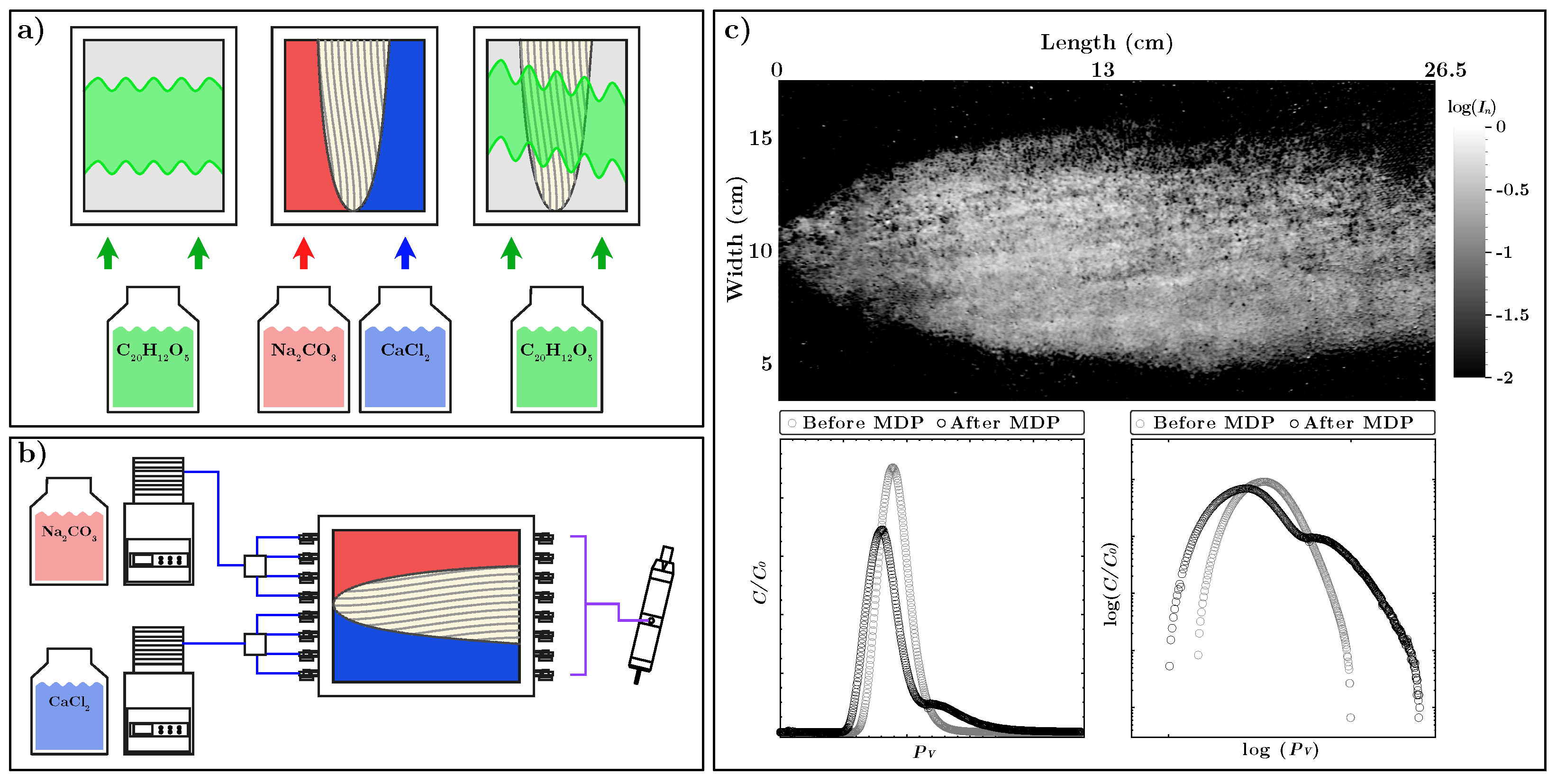
Figure 2.
a) Histogram of the calcite precipitation image. The x-axis displays the semi-quantitative precipitate amount as , while the y-axis shows the pixel frequency. The thresholds (Th) used for creating the dual permeability fields are indicated as follows: , , , . b, e) Dual-permeability fields obtained through image processing. The x and y axes represent the dimensions of the tank, where the x axis represents the length and the y axis represents the width of the experimental tank. The red color represents the non-precipitated areas, while the blue color represents the precipitated area.
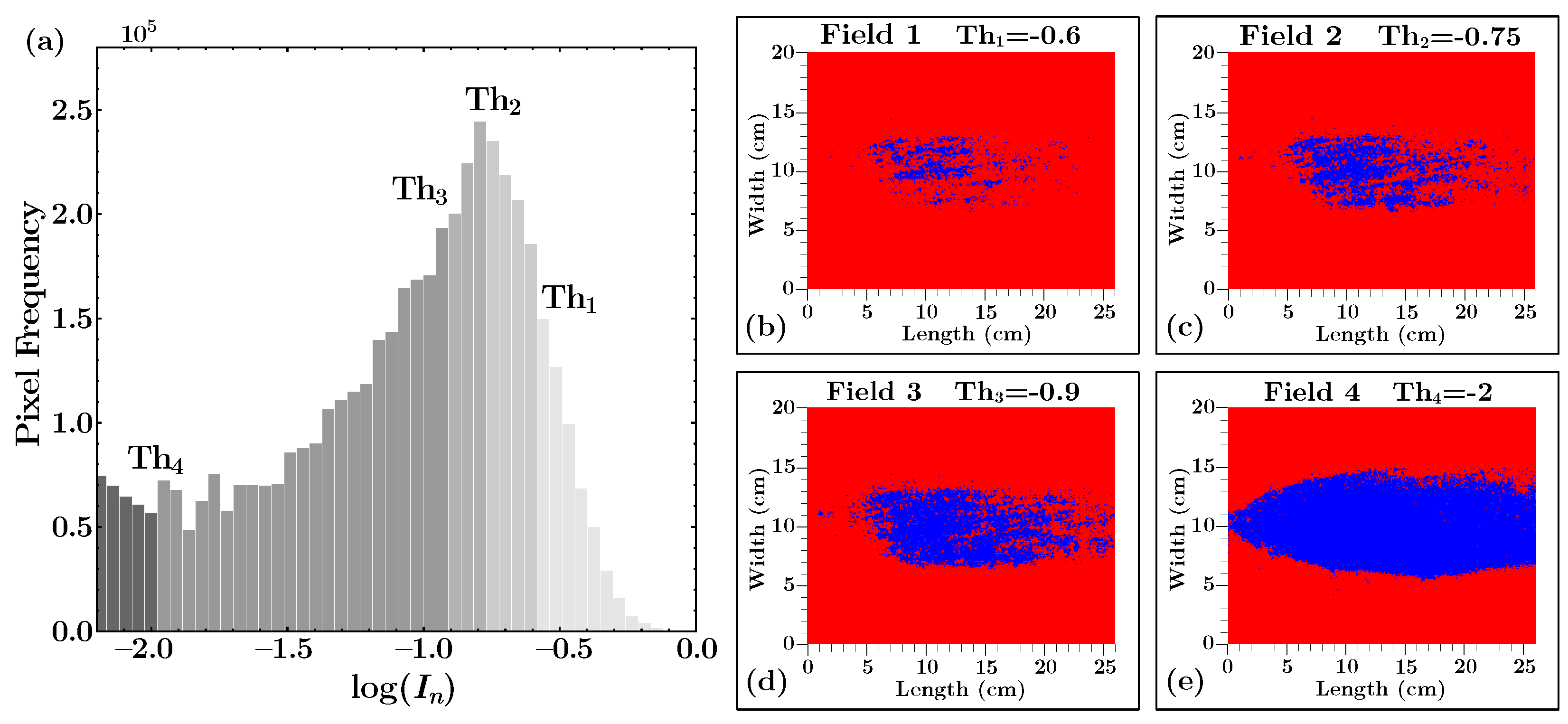
Figure 3.
Triple permeability fields obtained through the combination of the dual permeability fields. Both the (x) axis and the (y) axis represent the length of the experimental tank. Red represents areas unaffected by precipitation, green indicates areas affected by precipitation, and blue highlights areas with the highest precipitation.
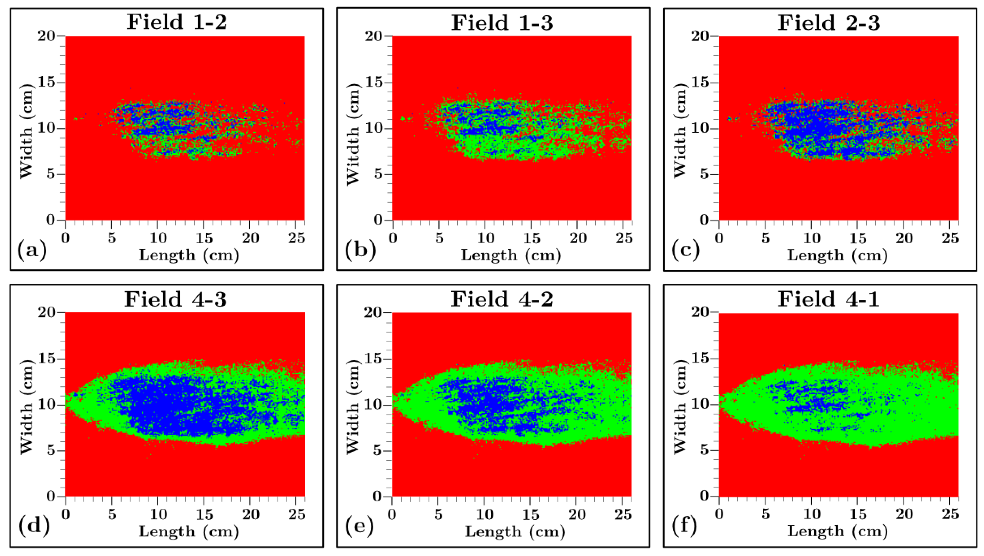
Figure 4.
Breakthrough curves (BTCs) comparison between the simulated and experimental results for the homogeneous synthetic aquifer. The segmented line represents the experimental results, and the solid line shows the simulated values from the model. a) Experimental and simulated breakthrough curves (BTCs), with concentration values normalized as C/ and time expressed in terms of pore volume . b) Breakthrough curves (BTCs) on a logarithmic scale.
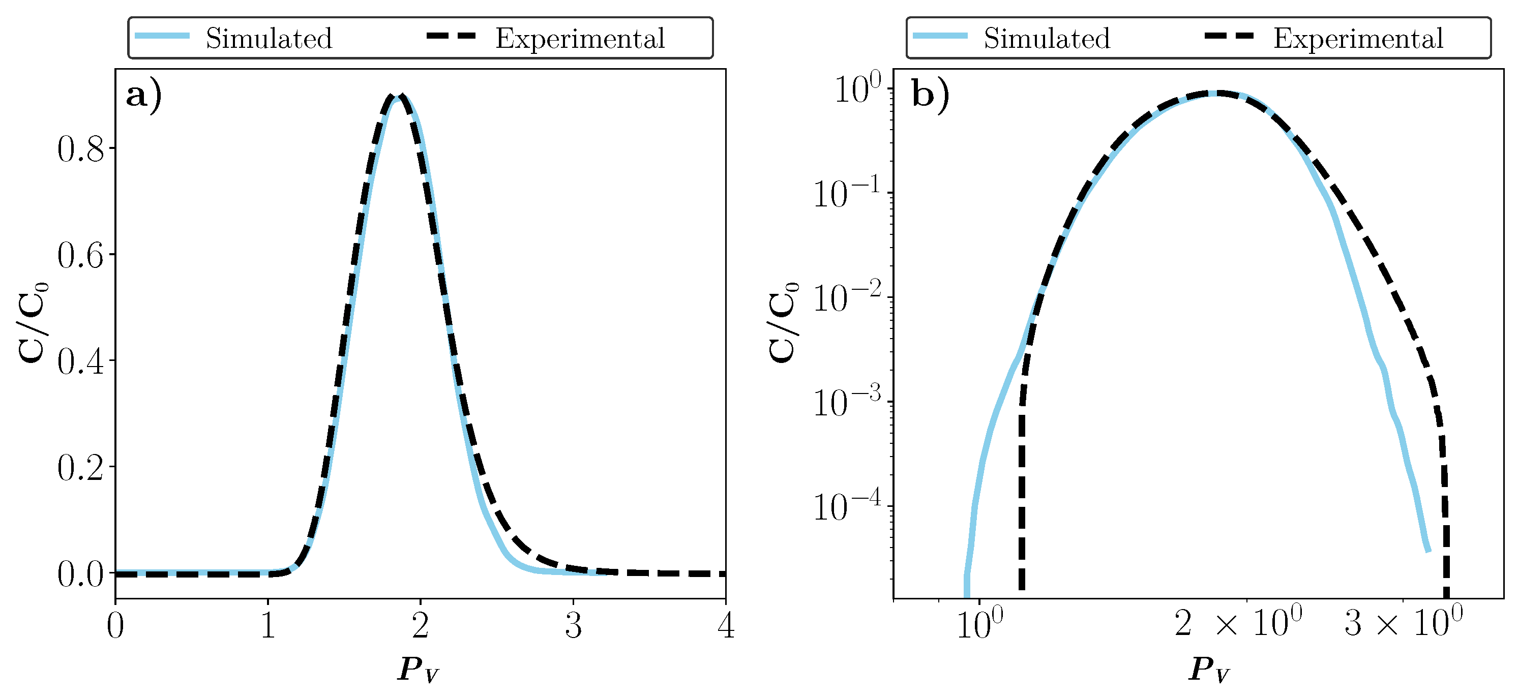
Figure 5.
Dual composite permeability fields implemented in the model, along with the simulated breakthrough curves (BTCs) obtained, with concentration values normalized as C/ and time expressed in terms of pore volume PV, also shown on a logarithmic scale.
Figure 5.
Dual composite permeability fields implemented in the model, along with the simulated breakthrough curves (BTCs) obtained, with concentration values normalized as C/ and time expressed in terms of pore volume PV, also shown on a logarithmic scale.
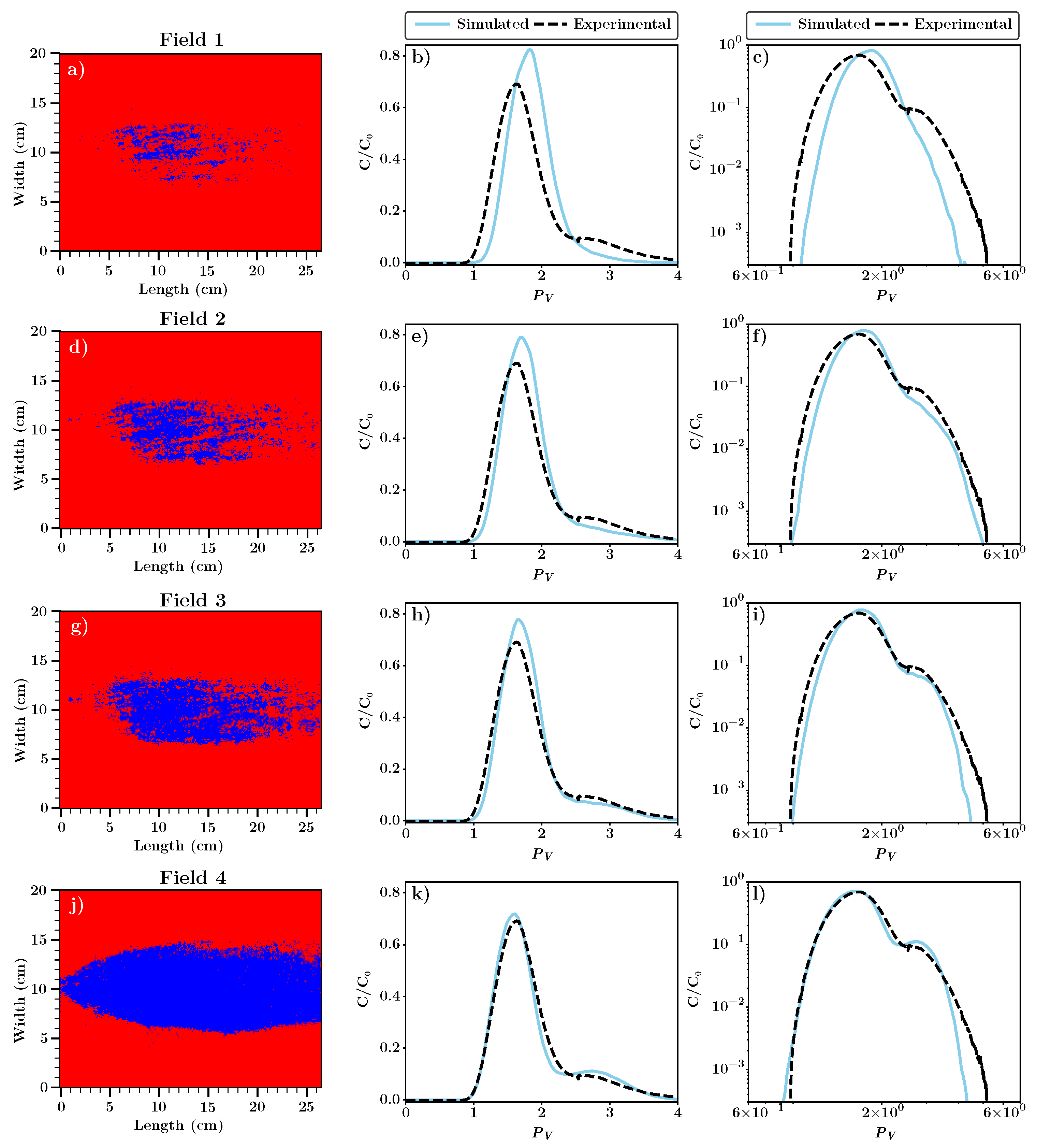
Figure 6.
Triple composite permeability fields implemented in the model, representing different scenarios of the internal structure of the precipitated layer, along with the simulated breakthrough curves (BTCs) obtained, with concentration values normalized as C/ and time expressed in terms of pore volume , shown on a logarithmic scale.
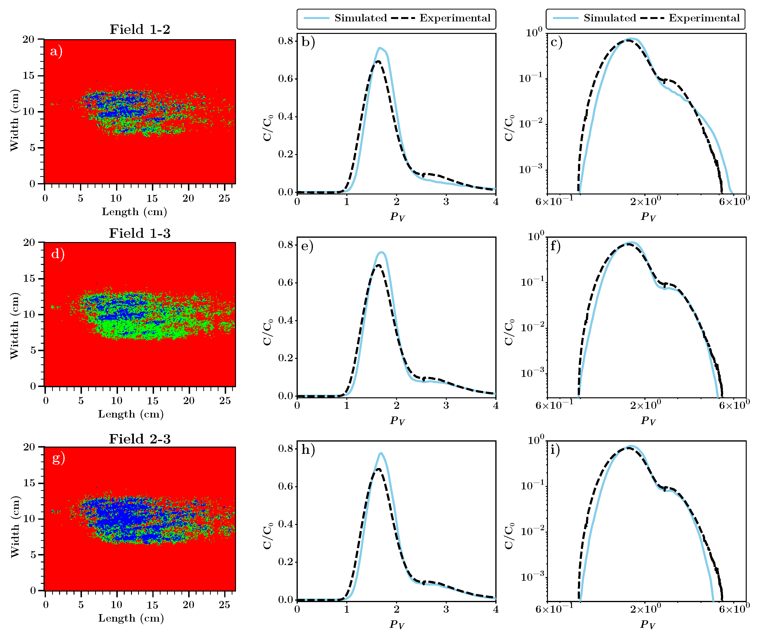
Figure 7.
Triple-permeability fields implemented in the model, representing the total area covered by precipitation and different scenarios to represent the internal structure of the high-precipitation zones, along with the simulated breakthrough curves (BTCs) obtained, with concentration values normalized as C/ and time expressed in terms of pore volume , shown on a logarithmic scale.
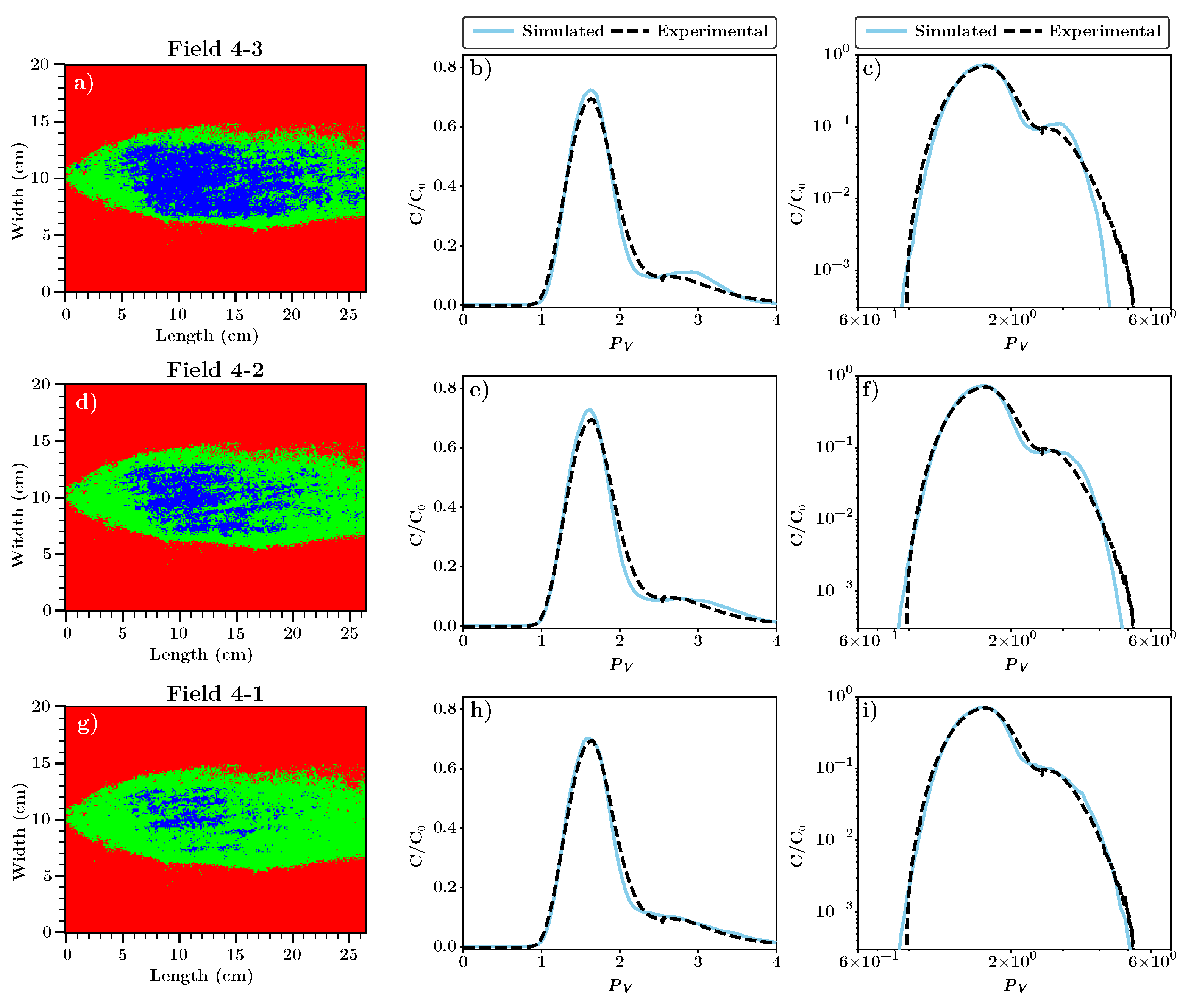
Table 1.
Experimental properties
| Symbol | Properties | Values | Units |
|---|---|---|---|
| Pe | Péclet number | 523 | – |
| Q | Total flow rate | m3/s | |
| D | Molecular diffusion (*) | m2/s | |
| d | Glass beads diameter | m | |
| v | Velocity | m/s | |
| Porosity | 0.34 | – | |
| A | Cross section | m2 | |
| Head difference | 0.014 | m | |
| L | Tank length | 0.265 | m |
| W | Tank width | 0.2 | m |
| H | Tank height | 0.01 | m |
| i | Hydraulic gradient | – | |
| Initial hydraulic cond. | 145.4 | m/d | |
| CaCl2 | 5 | mol/kgw | |
| Na2CO3 | 2 | mol/kgw | |
| cf | 145.4 | mg/l |
Note a: Information obtained from [54] (*).
Table 3.
Flow and transport model parameters
| Symbols | Parameters | Value | Units |
|---|---|---|---|
| W | Aquifer width | 0.2 | m |
| L | Aquifer length | 0.265 | m |
| H | Aquifer height | 0.01 | m |
| Q | Total flow rate | 0.0154 | m3/d |
| Initial porosity | 0.34 | - | |
| Initial hydraulic cond. | 145.4 | m/d |
Table 4.
Parameters obtained from the homogeneous synthetic aquifer.
| Symbol | Parameter | Value | Unit |
|---|---|---|---|
| Longitudinal dispersivity | 0.00265 | m | |
| Transverse dispersivity | 0.001 | m | |
| R2 | Coefficient of determination | 0.9939 | - |
| RMSE | Root mean squared error | 0.01946 | - |
Table 5.
Parameters obtained from the dual permeability models.
| Field | (m/d) | R2 | RMSE | AIC | |
|---|---|---|---|---|---|
| 1 | 8 | 0.055 | 0.7053 | 0.1022 | 998.66 |
| 2 | 17 | 0.117 | 0.9180 | 0.0539 | 279.52 |
| 3 | 37 | 0.254 | 0.9595 | 0.0379 | -116.33 |
| 4 | 60 | 0.413 | 0.9838 | 0.0239 | -634.57 |
Table 6.
Parameters obtained from triple composite permeability models representing different scenarios of the internal structure of the precipitated layer.
Table 6.
Parameters obtained from triple composite permeability models representing different scenarios of the internal structure of the precipitated layer.
| Field | (m/d) | (m/d) | R2 | RMSE | AIC | ||
|---|---|---|---|---|---|---|---|
| 1-2 | 22 | 13 | 0.151 | 0.089 | 0.934 | 0.048 | 151.22 |
| 1-3 | 45 | 20 | 0.310 | 0.138 | 0.964 | 0.035 | -203.80 |
| 2-3 | 65 | 30 | 0.447 | 0.206 | 0.955 | 0.039 | -82.17 |
Table 7.
Parameters obtained from triple composite permeability models, representing the total area covered by precipitation and different scenarios for the internal structure.
Table 7.
Parameters obtained from triple composite permeability models, representing the total area covered by precipitation and different scenarios for the internal structure.
| Field | (m/d) | (m/d) | R2 | RMSE | AIC | ||
|---|---|---|---|---|---|---|---|
| 4-3 | 88 | 48 | 0.605 | 0.330 | 0.988 | 0.019 | -890.46 |
| 4-2 | 78 | 32 | 0.536 | 0.220 | 0.985 | 0.022 | -725.68 |
| 4-1 | 73 | 17 | 0.502 | 0.117 | 0.991 | 0.017 | -1015.48 |
Disclaimer/Publisher’s Note: The statements, opinions and data contained in all publications are solely those of the individual author(s) and contributor(s) and not of MDPI and/or the editor(s). MDPI and/or the editor(s) disclaim responsibility for any injury to people or property resulting from any ideas, methods, instructions or products referred to in the content. |
© 2026 by the authors. Licensee MDPI, Basel, Switzerland. This article is an open access article distributed under the terms and conditions of the Creative Commons Attribution (CC BY) license (http://creativecommons.org/licenses/by/4.0/).
Copyright: This open access article is published under a Creative Commons CC BY 4.0 license, which permit the free download, distribution, and reuse, provided that the author and preprint are cited in any reuse.


