
Submitted:
26 January 2026
Posted:
27 January 2026
You are already at the latest version
Abstract
The hydropower plant together with its reservoir makes it possible to modify the natural flow regime. These changes can affect sediment transport dynamics and cause morpho-logical changes in the river. If the river is also used as a waterway, the operational scenar-io of the hydropower plant can have a significant impact on sediment deposition, thereby reducing its navigable depths and increasing the risk of vessel–riverbed collisions. In this study, a 2D hydrodynamic model of the Danube River downstream of the Gabčíkovo Hy-dropower Plant (GHP) in Slovakia was developed to evaluate the influence of operational scenarios on maintaining the required navigable depths and to determine the most suita-ble scenario in terms of fairway maintenance costs. The operational scenario of the GHP influences the amount of sediment deposited downstream of the plant. The volume of deposition in the critical ford was approximately 50% smaller under hydropeaking than under run-of-river operation. The increase in riverbed elevation during hydropeaking was 33% to 64% lower than under run-of-river operation. The study results indicate that this reach of Danube can remain navigable for a longer period without intervention (dredging), thanks to sufficient navigable depth maintained by erosion caused by hydropeaking, compared to run-of-river operation.
Keywords:
sediment transport
; 2D morphodynamic modelling
; hydropeaking
; MIKE 21
; navigation demands
1. Introduction
The Danube River constitutes one of the most substantial fluvial systems in Europe. Within the borders of Slovakia, the Danube extends for approximately 172 kilometres. Despite the relatively limited expanse of the Slovak reach of the Danube River, this section is of exceptional strategic importance. It functions as a pivotal hydrological and navigation corridor, linking Western and Southeastern Europe and constituting an integral segment of the trans-European waterway that connects the North Sea and the Black Sea via the Rhine–Main–Danube Canal. This navigation axis is formally designated as international waterway E80 and functions as one of the primary transportation arteries within the European inland navigation network. According to the European Agreement on Main Inland Waterways of International Importance (AGN), the Danube is classified as a Class VI waterway. For waterways of this class, the recommended minimum navigable depth is 2.7 meters, maintained continuously throughout the year. Ensuring compliance with this requirement necessitates sustained management interventions aimed at the stabilization of navigation depths. The Slovak reach of the Danube constitutes an alluvial middle reach of a perennial river, characterized by pronounced sensitivity to hydrological fluctuations and morphological dynamics. Sediment deposition, channel bed erosion, and shoal formation are among the most significant processes that influence channel morphology and hydraulic conditions. Absent measures to train and regulate the river, this reach would naturally evolve towards morphodynamic instability, leading to spatial and temporal variability in channel depths, restricted navigability, and heightened risk of vessel grounding, particularly under low-flow conditions. Consequently, ensuring sufficient navigable depths on the Danube is imperative for effective national water resources management and a priority within the broader international framework of Danube basin navigation and hydrological governance.
From the perspective of inland navigation, the Gabčíkovo Hydropower Plant (GHP) constitutes a pivotal infrastructure asset within the Slovak segment of the Danube River. The construction of the dam was driven by the dual objectives of enhancing navigation conditions in the region and generating electricity. Additionally, the dam was engineered to provide flood protection for the surrounding territory. Despite the implementation of hydraulic structures and river training measures, such as wing dikes, regular maintenance of the fairway remains necessary. This is primarily accomplished through the dredging of deposited sediments in the shoal reach (fords) downstream of the hydropower plant, where the Danube returns to its natural channel (see Figure 1)
The annual dredging costs in this reach are estimated to be approximately €3.6 million. Although shoal removal ensures rapid improvement of navigation conditions, its effects are temporary, requiring frequent repetition. In addition to increasing navigation maintenance costs, such interventions in the riverbed may also have considerable negative impacts on ecological conditions within the river and its floodplain. For this reason, both the International Commission for the Protection of the Danube River (ICPDR) and the Danube Commission, which oversees the harmonization of navigation conditions, emphasize that the maintenance of navigable depths must be carried out with regard to ecological interests and the protection of aquatic ecosystems. The primary focus is on addressing the underlying causes of sedimentation rather than merely remedying its consequences. Effective management of sediment transport is therefore essential not only for maintaining navigation safety and efficiency, but also for preserving ecological stability [1].
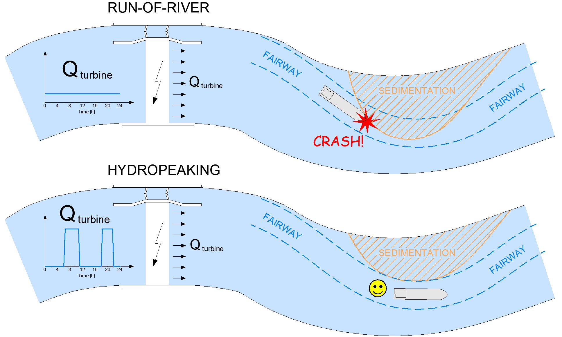
One approach to managing sedimentation processes is the controlled transport of sediments through the river flow management [2]. In [3], a novel term was introduced for this type of sedimentation control: morphogenic releases. This management approach necessitates the capacity to store water upstream of the designated river reach. The storage volume is then capable of regulating the natural discharge by increasing and decreasing the outflow from the reservoir. When such flow regulation is driven by starting turbines to cover peak electricity demand and shutting them down (or significantly reducing the discharge through the turbines) off-peak, it is referred to as hydropeaking. Conversely, the run-of-river hydropower plant operational scenario involves the plant’s output following the natural river discharge. This mode does not necessitate water storage. In the event that a limited storage volume (pondage) exists upstream of the hydropower plant, the plant can be operated in a modified run-of-river mode. Pondage permits only a negligible adjustment to the natural inflow; output undergoes a modest increase during periods of high demand and a slight reduction during off-peak hours [4]. Despite the construction of an impoundment with a volume sufficient for daily regulation of the natural discharge upstream of the GHP—meaning the plant could operate under a hydropeaking regime—it is currently operated in run-of-river, or more precisely, modified run-of-river mode. It is therefore worthwhile considering whether regulating the natural discharge through hydropeaking at the GHP could help reduce the costs of fairway maintenance.
As indicated by numerous studies, hydropeaking—defined as rapid and frequent fluctuations in the discharge of water downstream of a hydropower plant—exerts a direct or indirect influence on the morphology of rivers [5,6,7,8,9,10,11,12,13]. The recorded effects include an increase in suspended sediment load of up to ~25% and a substantial rise in sediment dispersion and mixing within the riverbed by up to 249.5% [14,15]. Fine sediments are known to accumulate primarily in dry zones that are flooded only during hydropeaking, whereas accumulation in permanently wetted areas is minimal [16]. In the adjacent reach of the river downstream, sediment transport predominates; however, further downstream, this phenomenon is primarily observed in relation to sand and very fine gravel, typically not beyond approximately 2 kilometres [17,18,19]. However, some studies have reported the strongest hydropeaking effects occurring up to approximately 17 km downstream, with mobilisation of fine fractions as well as coarser gravel [20]. Hydropeaking may lead to bank erosion and channel widening, while in other cases it may result in channel narrowing and morphological adjustments depending on the operational scenario [21,22].
Modelling sediment transport presents a complex issue, particularly in the context of alluvial channels of natural rivers, which represent two dynamic boundaries: the free surface and the riverbed. The dynamics between these two boundaries form an extremely complex system. The simulation of sediment transport, as with many other problems involving phenomena associated with the operation of hydraulic structures, relies on physical or numerical modelling [23]. Physical models are small-scale reproductions of real rivers that allow for detailed observation and measurement of complex phenomena that would be difficult to study in the field. However, the creation of physical models is both financially and time-consuming, and their use on a large scale or for solving long-term river morphology problems is often impractical. Numerical models offer the advantage of facilitating more rapid problem-solving and reducing costs in comparison to physical models. Numerical models allow for the simulation of sediment transport as a 1D, 2D, or 3D problem. The primary advantage of 1D models is their high computational speed, which renders them suitable for long-term simulations of relatively long river segments. However, the primary limitation of 1D models is that they neglect transverse bed variations in the river profile, which are crucial in many practical cases. In comparison to 1D models, 2D models offer the advantage of providing information about transverse flow fields, rendering them suitable for modelling river morphology in natural streams. 3D models have been shown to successfully solve the full set of Navier-Stokes equations, thereby providing high-resolution flow field simulations. At present, while 3D morphological models are extensively utilised for addressing local river hydraulics issues, they continue to be computationally intensive for large-scale river morphology applications. Consequently, 2D models are considered the most appropriate for river morphology simulations [1,24].
Various mathematical formulations are used to describe sediment transport. The Engelund-Hansen formulation is predicated on the theory of turbulent transport and is considered for the transport of fine to medium-grained sediments in rivers [25]. The Van Rijn formulation is based on an empirical approach and provides predictions for total sediment transport, including both suspended and bedload transport [26]. The Meyer-Peter Müller formulation is based on continuum theory and is commonly used for the transport of coarse-grained sediments [27]. The Engelund-Fredsøe formulation combines turbulent transport theory and continuum theory, making it suitable for a wide range of sediment grain sizes [28].
The equations employed for sediment transport calculations in morphodynamic models (e.g., Delft3D FM, BASEMENT 3, MIKE 21 ST, HEC-RAS 2D, RiverFlow2D) persist as the principal source of uncertainty and the key disadvantage of numerical modelling in comparison to physical models [1,24]. The minimisation of uncertainty in numerical models can be achieved through the availability of measured data for calibration and verification. A sediment-transport model is a multiparameter system that is prone to issues of equifinality, which occurs when the same outcome is achieved via different parameter combinations. This approach can yield a model that appears to be calibrated, yet it may produce predictions that are misleading and unrealistic. It is therefore essential to adopt an appropriate calibration strategy with a sound performance metric. In the context of hydro-sedimentary models, the calibration process is commonly initiated with a configuration that is exclusively hydrodynamic, thereby excluding the presence of sediment. Key hydrodynamic parameters include channel roughness, expressed via the Manning–Strickler coefficient ks, or, in some software, M (“Manning number”), turbulence parameters, and local losses at structures. The sediment-transport component is contingent upon the relevant sediment physical parameters (e.g., shear stress). The key input parameter for the sediment-transport model is the median grain size of the bed material, d50. The selection of the transport equation itself—and its internal coefficients, which some models permit fine-tuning—is also of critical importance. A preferred approach to calibrating transport formulations is the use of scaling factors. For instance, a sediment-transport scaling factor kb is employed to calibrate the output of the selected transport equation, thereby ensuring the optimal alignment with the measured sediment flux at the gauging cross-section.
Given the above, this study aims—using sediment-transport simulations in a numerical model—to demonstrate whether managing outflows from the GHP under a hydropeaking can maintain navigation depths in the fairway downstream of the plant (≥ 2.7 m as required by AGN) with fewer interventions compared to run-of-river operation, and thus reduce the volume of dredging (and hence the costs of fairway maintenance) while maintaining navigation safety.
In order to achieve this objective, a 2D numerical sediment-transport model was developed for a 50-kilometre reach of the Danube downstream of the GHP. The model was implemented in MIKE 21 ST environment developed by the Danish Hydraulic Institute (DHI). During the calibration and verification phases, four transport formulas were evaluated: Engelund–Hansen, van Rijn, Meyer-Peter–Müller, and Engelund–Fredsøe. The sediment transport was simulated for two bounding scenarios of outflow management through the GHP: run-of-river and hydropeaking. Based on the simulations, the 10-day cumulative increase or decrease of volume of deposited sediments in the fairway were determined for each operational scenario at the Danube’s critical ford at rkm 1798.5-1799.5 (bottleneck). The results were then used to assess which operational scenario of the GHP is more favourable in terms of the maintenance of navigation conditions in the reach under consideration.
This paper is organised as follows: Section 2 describes the study area and the numerical sediment transport model; Section 3 presents the results of the simulations of the GHP operational scenarios and their influence on maintaining the navigable depths in the fairway at the critical ford; finally, Section 4 and Section 5 provide the discussion, conclusions, and perspectives.
2. Materials and Methods
2.1. Study Area
The GHP, which was commissioned in 1992, is part of the large Gabčíkovo Project on the Danube River (see Figure 1). The GHP is a diversion-type hydropower plant with a total capacity of 8 × 90 = 720 MW, a total turbine capacity of 5,000 m³/s, and an average annual electricity production of 2,200 GWh. The maximum head is 23.6 m. Although the GHP currently operates in run-of-river mode, the Hrušov Reservoir has a storage capacity of 38.9 hm³ and can provide daily flow regulation such that the plant could operate in a hydropeaking with peak flow up to 5,000 m³/s (≈720 MW) for a minimum duration of four hours. The intake channel measures 28 km in length, while the waste channel extends for 8 km. Two shiplocks, each measuring 34.0 × 275.0 m, are utilised to surmount the plant’s head. International navigation on the Danube is principally facilitated through the intake and waste channels. The average annual inflow to the Hrušov reservoir is about 2,000–2,100 m³/s, though during floods, it can reach up to 10,000 m³/s. The lowest inflows are approximately 700 m³/s, while a discharge in the range of from 200 to 450 m³/s must be maintained in the old Danube riverbed, depending on the season. Throughout the season, the discharge remains constant. Its solid contribution consists mainly of suspended fines (silt and fine sand), which are transported along the entire studied river reach and partly deposited in the floodplain. The discharge in the Moson Danube, which joins the Danube near Kližská Nemá, is constant at 40 m³/s. Its solid contribution is regarded as negligible. The highest flows in the Danube River occur in the spring and early summer due to snowmelt in the Alps and spring rains, while low water levels are typical in the autumn and winter months. During this period, in the shoal reach from 12 to 27 km downstream of the GHP, vessel groundings on the fairway bed are frequently recorded, leading to towline breakage and loss of control of the vessels. The reach of the Danube downstream of the GHP represents typical problems associated with the damming of an alluvial river flow, where the continuity of sediment movement is interrupted by the constructed hydraulic structure. The median grain size of the bed material is d50 = 9 mm. Sediments settle in the impoundment reservoir above the dam, and the water flowing below the dam is deprived of transported bed material. Instead of compensating for the eroded bed material with incoming sediments, the downstream of the dam is predominantly subjected to erosion, leading to the sinking of the riverbed [29,30]. The medium to long-term morphological changes in this reach of the river caused by the construction of the Gabčíkovo Dam are well documented in [31,32]. The longitudinal profile of the Danube (the deepest part of the riverbed) clearly demonstrates that during the first 10 years of GHP operation, which began in 1992, the most dynamic changes occurred between the GHP and Medveďov (from 0 to 12 km downstream of the GHP), and later downstream of Medveďov. The riverbed in this reach underwent a significant deepening, with an estimated bed degradation of approximately 4 - 5 m (with local erosion reaching up to 7 m). In the reach from 20 to 40 km downstream of the GHP, the formation of several-meter-high sediment deposits was observed. In the reach from 40 to 50 km (up to Komárno), milder morphological changes were recorded, and the downstream of the Komárno remained relatively stable. Despite the observed decline in the intensity of riverbed deepening and the stabilization of the morphology in the GHP – Sap reach (from 0 to 8 km downstream of the GHP), the process of bed degradation with subsequent redeposition of the eroded material has not yet ceased. The current level of the Danube riverbed indicates the deposition of sediments in the from Medveďov–Kližská Nemá reach (from 12 to 27 km downstream of the GHP). This trend may exert an adverse impact on groundwater levels, substantial water discharge, and is already exerting a deleterious effect on navigation conditions in fairway. From 1992 to 2024, the total volume of dredged bed sediments was 2,584,000 m³. When converted to current price levels, the cost of dredging is approximately €117 million.
2.2. Numerical Model
2.2.1. DHI Mike 21 Model
In order to achieve the objective outlined in Section 1, the 2D model Mike 21 ST (Sand Transport) was utilised for the purpose of simulating morphological development. This model is capable of calculating the transport of non-cohesive materials. The foundation for sediment transport modelling is the hydrodynamic model of the study area, which was created using The DHI’s Mike 21 software is a comprehensive solution for 2D free-surface flow modelling. It employs the finite volume method for discretisation, dividing the model geometry into non-overlapping elements. The model is based on solving the 2D Reynolds-averaged Navier-Stokes (RANS) equations, integrated over depth. The dependent variables of the system are referenced to the centre of each element. A detailed mathematical formulation of the model is provided in [33,34].
Sediment Transport Module – Mike 21 ST (Sand Transport)
The calculation of sediment transport using Mike 21 ST is based on hydrodynamic conditions and sediment properties. Sediment transport modelling is divided into bedload transport and suspended sediment transport. The primary factor influencing navigation conditions in the studied reach of the Danube River is bedload transport (i.e. sediment moving along the riverbed). In the absence of external sediment sources, it is assumed that all sediment in the system originates from the riverbed, and a so-called equilibrium description of sediment transport is considered. Bedload transport is primarily dependent on shear stress (τ), which governs the movement of sediment along the riverbed.
where ρw is the density of water [kg/m³], g is the gravitational acceleration [m/s²], v is the flow velocity [m/s], and C is the Chezy roughness coefficient [m0.5/s]. To calculate the change in bed elevation ∂Z/∂t, the sediment continuity equation (2) is used, ensuring mass conservation of bedload transport.
where n is the porosity of the bed material [[-], Z is the bed elevation [m], t is time [s], Sx and Sy are the sediment transport rates in the x and y directions [m²/s], and ΔS represents an external sediment source. The bed elevation at time step i can be determined using equation (3).
where Δt is the time step of the simulation.
Sediment transport is a process that can be calculated, with the calculation taking into account gravitational effects forced by longitudinal and transverse bed slopes. Furthermore, if helical flow is included in the model, the calculation will adjust for the deviation of the bed shear stress from the mean flow (see Figure 2).
In order to calculate the amount of sediment transport in the direction of the transverse slope (n), the Mike 21 ST model utilises the following relationship (4):
where G is the calibration factor for bed slope (for natural rivers, = 1.25), a is bed slope exponent (for natural rivers, = 0.5), tan δs is the change in shear stress direction caused by the secondary flow forces, Sbl is the bedload sediment transport [m²/s], and θ is the Shields parameter (according to (6)).
The sediment transport in the direction of flow (Ss) is expressed by the equation (5).
where α is the calibration parameter (ranging from 0.2 to 1.5).
To predict the initiation of sediment transport, each transport equation uses the Shields parameter (θ). It is a dimensionless number that defines the ratio between shear stress and the gravitational force acting on a particle.
where τ is the shear stress [Pa=N.m⁻²], ρ is the density of water [kg/m³], ρs is the density of bed material [kg/m³], and d₅₀ is the median grain size of the bed material [m].
The calculation of bedload sediment transport (Sbl) is possible through the utilisation of four equations available in Mike 21 ST: Meyer-Peter Müller, Van Rijn, Engelund-Hansen, and Engelund-Fredsø. However, it should be noted that the applicability of each of these equations is constrained to a specific range of conditions and grain sizes, for which they were originally derived.
2.2.2. Model Setup
The numerical model encompasses the Danube River from rkm 1818 - GHP to rkm 1768 – Komárno, was developed within the Mike 21 FM environment. The computational scheme of the numerical model is delineated in Figure 3.
The model encompasses a total length of 50 km. The width of the modelled area between the two flood-protection levees (including the floodplain) ranges from approximately 0.4 km to 2.8 km, while the main channel is about 0.4–0.6 km wide. The total modelled area is 65.4 km². A bathymetric survey of the riverbed bed was conducted in 2013 using a single-beam echo sounder. Cross-sections were measured at 50-meter intervals along the modelled river reach, resulting in a dense, continuous dataset of depth points. Wing dikes (groynes) were surveyed in the same year using GPS. The floodplain topography is based on airborne LiDAR (laser scanning) acquired in 2013. The LiDAR dataset is available for the entirety of Slovakia.
The model’s computational mesh is a combination of structured curvilinear and unstructured triangular meshes. The riverbed topography, inflows, and branches are discretised with a curvilinear mesh, while the uneven terrain in the floodplain is represented by a triangular computational mesh (see Figure 4). The computational mesh is composed of approximately 250,000 elements. In order to circumvent the occurrence of non-physical results, the mesh was generated in such a manner that the spatial expansion ratio between adjacent elements in a given direction remained less than 10. The area of the smallest element is 20 m², while the largest is 2,500 m². In the primary channel, rectangular elements measuring 20 × 10 m are employed, while the floodplain is delineated by triangular elements with an average area of approximately 1,000 m² (equivalent to triangles with side lengths of approximately 45 m).
2.2.3. Hydrodynamic Model of Surface Water Flow and Calibration
The spatial extent of the Hydrodynamic Model of Surface Water Flow is equivalent to that of the comprehensive numerical model delineated in Section 2.2.2 (refer to Figure 3). The riverbed and its branches are discretised with a quadrilateral mesh comprising 130,000 elements, while the floodplain is represented by triangular elements with 120,000 elements. The spatial extent of the modelled area is constrained to the region in which reliable boundary conditions for the simulation can be specified. In this case, the upstream boundary condition is defined by the time series of discharge through the GHP turbines (GHP Flow), the inflow from the Old Danube riverbed (Old Danube Riverbed Flow), and the inflow from the Moson Danube (Moson Danube Flow). The downstream boundary condition is determined by the rating curve at rkm 1768 – Komárno, which is routinely evaluated by the Danube River authority. This curve serves as the initial suitable downstream boundary condition for simulations conducted downstream of the GHP. The hydrodynamic model has thus been demonstrated to possess the capacity to simulate water levels and discharges in a 50-kilometer reach of the Danube under both steady and unsteady flow conditions caused by hydropeaking at the GHP.
In instances where the quantification of sediment transport within a specific river reach is of interest, it may not be feasible to reliably define the flow boundary conditions for the simulation. In such scenarios, the hydrodynamic model area may extend beyond the boundaries of the sediment transport area. In such a case, the hydrodynamic model is employed to compute the flow boundary conditions for the sediment transport simulation in the Mike 21 ST module.
To simulate sediment transport under conditions of highly unsteady flow, it is essential to attain the highest possible degree of accuracy across the entire range of flows [35]. For the calibration, a procedure was selected that seeks to minimize the overall deviation from all measured data across the flow range, based on a set of evaluation criteria: Root Mean Square Error (RMSE), Mean Absolute Error (MAE), and R² (R-Squared). The calibration process involved iteratively modifying the Manning number (M) — representing channel roughness — calculating water levels, and comparing them with measurements until a sufficiently good match with the measured water levels was achieved. The boundary conditions for the model were established based on the identification of three real-world flow scenarios with steady flow (see Table 1). Three flow scenarios represent low-, medium-, and high-flow conditions, chosen to cover the entire range of discharges realized under the run-of-river operation of the GHP, which produces steady-flow conditions in the Danube River. The corresponding measured water levels are provided in Table 2. The results of the hydrodynamic model calibration are presented in Section 3.1.
2.2.4. Sediment Transport Model and Calibration
The sediment transport model encompasses the Danube River from rkm 1810 - Sap to rkm 1791 - Kližská Nemá, corresponding to km 8–27 of the numerical model domain (see Figure 3). The area of the model is 30.91 km², and the computational mesh contains 82,046 elements. The sediment transport model area encompasses only the river reach that is characteristic of the shoal formation process (deposition area). Its length is 19 km. The sediment transport area is therefore smaller than the hydrodynamic model area. Consequently, the hydrodynamic surface water flow model described in Section 2.2.3 is used to compute the flow boundary conditions for the sediment transport model.
The delineation of the sediment transport model area was conducted with the understanding that this reach of the Danube plays a pivotal role in its navigability (see Figure 1). Excessive sedimentation in this reach increases maintenance costs for the fairway and raises the risk of vessels becoming stranded if adequate navigation conditions are not ensured. The sediment transport model area also includes the critical shoal reach of the Danube (bottleneck) located between rkm 1798.5 and 1799.5 (approximately 19 km downstream of the GHP) – see Figure 4 and Figure 5. This reach is crucial for maintaining the required navigation conditions on the Danube and is the area where the largest dredging volumes are carried out in order to achieve the required minimum navigable depths. In the following, this reach is used as the reference reach for assessing the 10-day cumulative increase or decrease of volume of deposited sediments in the fairway for the individual GHP operational scenarios.
Another evaluation parameter for assessing the influence of the GHP operational scenarios on sediment transport will be the increase or decrease of the riverbed elevation at the critical ford, which provides information on the spatial distribution of sediment in the fairway. From a navigation perspective, this is even more significant than the information on the total amount of volume of deposited sediments in the fairway itself. It was necessary to define the method for determining the riverbed elevation in advance. Unlike rock sills, fords are not static river formations; their location, height, and shape change over time due to sediment transport dynamics. Therefore, an approach was selected that captures this variability. The evaluation was based on a set of five longitudinal profiles taken at 30-meter intervals: one along the axis of the fairway, two parallel profiles at 30 meters from the axis, and two additional profiles at 60 meters from the axis at the edges of the fairway (see Figure 5). The riverbed elevation in the fairway at the critical ford is then understood elevation of the ford crest, i.e. the maximum riverbed level in the corresponding longitudinal profiles.
The median grain size (d₅₀) of the bed material is the key input parameter for the sediment transport model. The studied reach of the river is rich in measurements and analyses from several studies, which provided data for calibration [31,32,36]. The median grain size in the model is assumed to be d₅₀ = 9 mm. The porosity (Φ) is defined a priori as 0.40, which is the best estimate for well-sorted fine to medium gravel [37,38]. The acceptable range for the calibration factor for sediment transport (kb) is from 0.5 to 2.0. The distribution of simulated sediment transport was then compared with measurements at the rkm 1795.58 cross-section (22.15 km downstream of GHP) for the purpose of calibration, and a relationship for calculating of sediment transport rate from flow (in kg/s) was derived for this cross-section [36].
This profile was chosen because it is the location of an extensive sediment transport measurement campaign conducted during 2000, 2001 and 2002 [39]. A total of 71 bedload sampling measurements were performed, covering a discharge range of Q = 972 – 4,745 m³/s, while a threshold discharge of incipient bedload motion in this reach is roughly 900 m³/s. The measurements were conducted using a basket-type bedload sampler similar to the Ehrenberger (1931) model, from the survey vessel. The measurement cross-section included six verticals, located at distances from the left bank as follows: 50, 80, 130, 180, 240, and 280 m. At each vertical, 10 replicate measurements were taken and averaged to minimize random errors. The grain size distribution of the bedload samples was found to be nearly uniform across the section. On average, the median grain size was d₅₀ = 9 mm, with d₁₀ = 5 mm and d₉₀ = 18 mm.
The calibration process consisted of tuning the sediment-transport scaling parameter kb and the selection of the most suitable formula for describing sediment transport. Calibration flows were selected to coincide with flows where the greatest number of sediment samples were collected in the cross-section (~1,000 m³/s < Q < ~3,000 m³/s). The upper flow boundary condition of the sediment transport model at rkm 1810 – Sap (8 km downstream of GHP) was considered, with calibration flows of 1,250 and 2,750 m³/s, and calibration values for sediment transport rate Qs were 4.25 and 20.16 kg/s (according to (7)). The lower flow boundary condition is defined by the rating curve derived from the hydrodynamic model at the rkm 1791 – Kližská Nemá (27 km downstream of GHP). The upper boundary condition of the sediment transport model was solved using the fixed bed method, while the lower boundary condition was defined by a zero-sediment transport gradient. The set of calibration computations consisted of 20 models. Five models with varying the sediment-transport scaling factor kb (0.5, 0.75, 1.0, 1.5, and 2.0) were applied for each the transport equations: Engelund and Hansen, Van Rijn, Engelund and Fredsøe, and Meyer-Peter-Müller for flows of 1,250 and 2,750 m³/s. The models were evaluated based on the assessment criteria RMSE, MAE, and R² in the same manner as outlined in Section 2.2.3. The results of the sediment transport model calibration are presented in Section 3.2.
2.2.5. Model Uncertainty
Complex models, such as the sediment transport model, require quantification of uncertainty in order to ascertain the extent to which the model’s results are backed by real data and also the accuracy with which the model represents the actual phenomenon [40,41]. The precise determination of the uncertainty of the model’s results can only be performed if the degree of uncertainty of all input parameters is known, and the tolerated variance of the results is defined. The causes of uncertainty in model results can be categorised into three groups: variability of the physical parameters included in the model; inaccuracies and sporadicity of the data obtained; and modelling errors.
In this study, the issue of uncertainty in the model is addressed by employing the First-order second-moment (FOSM) method. This method is a widely utilised engineering approach for quantifying model uncertainty. To calculate the prediction interval, the mean and variance of the input parameter are determined, and the output parameter is extrapolated based on these values. Generally, the FOSM can be expressed as follows:
where Z is the modelled parameter, pi are input parameters, μi are the mean values, and σ2 is the variance of the input parameters. FOSM is a computationally very efficient method, requiring only one simulation per input parameter.
In the event of the variance of output parameters being too great, the model’s uncertainty is either overestimated or underestimated. The FOSM method is predicated on the assumption that input parameters follow a normal distribution, and that the phenomenon under consideration is linear. However, it is well-documented that sediment transport is generally a nonlinear phenomenon (see, for example [40,42,43,44]. Consequently, FOSM can only provide fully reliable results if the observed phenomenon is quasi-linear, and if the variance of input parameters is sufficiently small. Despite its limitations, the FOSM method remains a preferred approach in practice, not due to its perceived simplicity or computational efficiency, but rather because of its superior performance when confronted with methods that are computationally intensive.
A critical parameter for determining the model uncertainty is the mean grain size of the sediment, d50 = 9 mm. Utilizing advanced uncertainty analysis methods with algorithmic differentiation and Monte Carlo simulation, it was ascertained that the mean grain size (d50) contributes up to 25% of the variability of the model’s results. The measurement uncertainties in grain size are attributed to natural variability and measurement errors, and are represented in the model by a standard deviation of 2.204 mm. The impact of these uncertainties on the model output is quantified by a 95% prediction interval, which is derived through uncertainty analysis. This analysis provides a more robust understanding of the model’s predictability, thereby enhancing the reliability and interpretability of the calculation results.
2.3. The GHP Operational Scenarios
The present study assesses the sustainability of navigation conditions in the Danube fairway using simulations with a 2D morphodynamic model. The analysis is conducted for two limiting operational scenarios of the hydropower plant in terms of regulation of the natural flow regime, namely run-of-river and hydropeaking operation. The simulated period for both scenarios was 10 days, during which an average daily inflow to the Hrušov reservoir of 2,900 m³/s and a diversion of 400 m³/s to the Old Danube Riverbed were considered, meaning that the average flow available for the GHP is 2,500 m³/s.
In the case of run-of-river operation, a turbine discharge of 2,500 m³/s through the GHP was considered. In the case of hydropeaking, peak flows of 5,000 m³/s lasting 4 hours were assumed, utilising the storage volume of the reservoir, which amounts to 38.904 hm³. Off-peak flows of 2,000 m³/s so that over 24 hours the daily regulation cycle of the natural flow was balanced. Thus, the total volume of water passing through the GHP turbines was the same for both the hydropeaking and run-of-river operation. Figure 6 shows the discharge hydrographs for both GHP operational scenarios. Each hydrograph represents the upstream flow boundary condition (“GHP Flow” at rkm 1818) used to simulate the surface water flow downstream of the GHP with the hydrodynamic model. The other flow boundary conditions for both scenarios were the inflows to the Danube, “Old Danube Riverbed Flow = 400 m³/s” and “Moson Danube Flow = 40 m³/s” (see Figure 3). The downstream boundary condition of the hydrodynamic model was the rating curve at rkm 1768 – Komárno.
3. Results
3.1. Surface Water Flow Model Calibration
In the reach rkm 1810 to rkm 1800, corresponding to km 8–18 of the numerical model domain, the roughness in the deeper part of the channel is lower than in the bank zone, ranging from M=25 m¹/³/s to M=42 m¹/³/s. Beyond rkm 1800, the cross-sectional distribution of roughness remains uniform, ranging from M=35 m¹/³/s to M=49 m¹/³/s. The range of water level differences between the calibrated model and the measurements taken at the Medveďov gauge was from -0.13 m to +0.03 m, and at the Kližská Nemá gauge from -0.1 m to +0.05 m (see Table 3).
3.2. Sediment Transport Model Calibration
The differences in the simulated and measured values of sediment transport rate Qs are clearly visible in their graphical comparison in Figure 7 and in Table 4. The triangular symbols in Figure 7 represent the measured values of sediment transport in the cross-section at rkm 1795.85 for the years 2000 to 2022, obtained using the method described in Section 2.2.4. The findings indicate that the Engelund and Hansen model produces significantly overestimated Qs values for both flows. For Q value of 2,750 m³/s, the range of sediment transport is from 71.08 kg/s (kb=0.5) to 292.45 kg/s (kb =2). For Q =1,250 m³/s, the sediment transport ranges from 17.97 kg/s (kb =0.5) to 72.08 kg/s (kb =2). it is evident that the prediction errors of this model are relatively high, and its R² values are negative, indicating poor data fitting. The Engelund and Fredsøe model produces significantly higher Qs values than the Engelund and Hansen model, with Qs ranging from 191.95 kg/s (kb =0.5) to 962.12 kg/s (kb =2) for Q=2,750 m³/s. A similar trend is observed for Q =1,250 m³/s. However, the prediction errors are larger than in the Engelund and Hansen model, and the R² values are negative, suggesting that this model also poorly fits the data. The Van Rijn model produces Qs values ranging from 25.87 kg/s to 109.72 kg/s for Q=2,750 m³/s, and from 3.43 kg/s to 13.84 kg/s for Q=1,250 m³/s. The prediction errors (RMSE and MAE) are relatively low. The model demonstrates positive R² values of 0.74 for kb=0.5, signifying a satisfactory data fit. The Meyer-Peter Müller model exhibits minimal prediction errors and positive R² values of 0.6 for kb=0.5 and R²=0.89 for kb=0.75, indicating an adequate fit to the measured data.
It is acknowledged that both transport equations are commonly utilised and validated for rivers exhibiting conditions analogous to those observed in the designated reach of the Danube. In order to substantiate the credibility of these models, a comparative analysis is presented in Figure 8, which utilises the Van Rijn and Meyer-Peter Müller transport equations to illustrate the congruence between measured and simulated sediment transport distributions in the cross-section at rkm 1795.58. The Van Rijn equation is known to be suitable for use in complex and variable environments (e.g., natural flow curvature, sharp changes in flow due to hydropeaking) [26], and so the Van Rijn (1984) model with kb=0.5 was selected for further analysis.
3.3. The GHP Operational Scenarios Effect on Sediment Transport
The influencet of the GHP operational scenario (described in Section 2.3) on sediment transport in the Danube reach downstream of the dam was evaluated using simulations with the numerical sediment transport model described in Section 2.2.4. The morphological changes were compared as follows: (i) 10-day cumulative increase/decrease of volume of deposited sediments in the fairway at the critical ford rkm 1798.5-1799.5 (see Section 3.3.1), and (ii) 10-day cumulative increase/decrease of riverbed elevation in the fairway at the critical ford (see Section 3.3.2). Based on the results, it was possible to assess whether, in terms of maintaining the required navigable depths (≥ 2.7 m according to AGN) in the Danube reach under consideration, the run-of-river operational scenario or hydropeaking operation is more advantageous.
3.3.1. Volume of Deposited Sediments in the Fairway at the Critical Ford
As demonstrated in Table 5, the modelling of the Danube reveals that, in the case of both run-of-river operation and hydropeaking, sedimentation of bed material occurs in the reach of the Danube under consideration. However, during hydropeaking, the bedload volume in the fairway is approximately half that observed in run-of-river operation. After 10 days of simulated run-of-river operation, the sediment volume in the fairway at the critical ford is about 184 m³ greater than during hydropeaking. The modelling results are also provided for the 95% prediction interval (PI95%), offering a broader view of the variability of sediment transport under the given conditions. Figure 9 illustrates the temporal development of volume of deposited sediments in the fairway at rkm 1798.5–1799.5 during the simulation period.
3.3.2. Riverbed Elevation in the Fairway at the Critical Ford
Under run-of-river operation, the maximum riverbed elevation within the monitored longitudinal profiles (as shown in Figure 5) after 10 days reached 104.18 m a. s. l. at -60 m from the axis of the fairway, 104.27 m at -30 m, 104.71 m on the axis, 105.00 m at +30 m, and 105.09 m at +60 m (see Figure 10). The maximum allowable riverbed elevation is 104.69 m a.s.l., which corresponds to the level at which the threshold depth of 2.7 m is still ensured at the minimum navigable discharge in this reach of the Danube, i.e. 1,000 m³/s. Under hydropeaking operation, the maximum riverbed elevation after 10 days reached 104.17 m at −60 m from the fairway axis, 104.27 m at −30 m, 104.71 m at the axis, 104.98 m at +30 m, and 105.05 m at +60 m. In Table 6, these values are converted into water depths for the minimum navigable discharge. The depths that are less than the threshold depth of 2.7 m are marked in red. However, the above data clearly show that the required navigable depths were not ensured in some of the monitored longitudinal profiles even at the initial time of the simulation.
A comparison of the scenarios shows that in both cases, after 10 days, some locations within the critical ford experience deposition and others erosion (see Figure 11). However, the maximum riverbed elevations reached within the fairway at the critical ford are lower under hydropeaking than under run-of-river operation. In the longitudinal profile at +30 m, the difference is 1.9 to 2.8 cm (~33%), and in the profile at +60 m, the difference is 3.4 to 3.8 cm (~47 to 64%) compared to the run-of-river operation (see Table 7).
4. Discussion
The results of the numerical modelling showed that the operational scenario of the GHP affects sediment transport and the morphological development of the critical ford of the Danube at rkm 1798.5–1799.5. With the same daily volume of released water, ten days of hydropeaking resulted in approximately half the volume of newly deposited sediments in the fairway compared with run-of-river operation. The estimated 95% prediction intervals of the model further underscore the substantial impact of the selected operational scenario on the sedimentation conditions within the investigated ford. From a mechanical point of view, the results can be interpreted such that, under run-of-river operation with a steady discharge of 2,500 m³/s, conditions favourable for material accumulation prevail in the area of the critical ford. In contrast, hydropeaking with discharge peaks of 5,000 m³/s lasting 4 hours and a reduced discharge of 2,000 m³/s off-peak periods produces short but repeated episodes of increased shear stress that are capable of remobilising part of the already deposited sediments from the crest of the ford. As a result, the net increase in sediment within the fairway is smaller, although over the wider reach there may be a redistribution of erosional and depositional zones.
When assessing navigation conditions, not only the volume of deposited sediments is important, but also the maximum riverbed elevation across the fairway width. The computations showed that the rise in riverbed level at the critical ford is approximately one-third to two-thirds smaller under hydropeaking than under run-of-river operation, with the difference being most pronounced in the right-bank part of the fairway. Although these differences are “only” on the order of centimetres, in an environment where the required minimum depth is 2.7 m and depths in the shoal reaches fall below this threshold, even such differences have a direct impact on the number of days with restricted navigability and the frequency of dredging interventions required. At the same time, it should be emphasised that even under the more favourable hydropeaking scenario the required depth of 2.7 m is not ensured across the entire cross-section of the ford, so technical interventions remain indispensable.
From a water-management perspective, the results suggest that flow regulation by hydropeaking may serve as a complementary tool for morphological management of the fairway. Potential benefits include a reduction in the volume of dredged sediment and thus in the financial costs of maintaining navigable depths, as well as a reduction in the negative ecological impacts associated with frequent disturbance of the riverbed. At the same time, however, the very mechanism that enhances the river’s “self-cleaning” capacity and sediment redistribution is also the source of unsteady flow and translation waves, which are associated with adverse effects on bank erosion, fish and macrozoobenthos habitats, water quality, and on navigation safety itself. Changes in flow velocity and direction can complicate vessel manoeuvring, increase fuel consumption and cause delays, with the transition from open water to the shiplock approach being particularly critical. Dynamic phenomena such as positive and negative translation waves generated by sudden discharge changes can lead to loss of vessel manoeuvrability, collisions with banks, piers or other vessels, and pose a risk to moored ships (breaking of mooring ropes, anchor dragging). Therefore, any consideration of modifying the operation of the GHP must be based on an integrated assessment in which the morphological benefits and energy demands are evaluated in parallel with ecological constraints and the requirements for a safe flow and velocity regime for navigation.
The limitations of the applied approach must also be acknowledged. The model is depth-averaged (2D), uses a homogeneous representative bed grain size and considers only non-cohesive material. The 10-day simulation horizon captures the short-term response of the ford to a change in operating regime, but does not represent long-term morphological evolution. Only two limiting operational scenarios and a single initial morphological configuration were considered. Actual operation, influenced by electricity demand and hydrological variability, may generate different combinations of waves than those tested in this study. For these reasons, the obtained results should be understood as a consistent but still scenario-based estimate of the potential of flow regulation to improve navigation parameters, rather than as a definitive proposal for an optimal operational scenario. Further research should therefore focus primarily on long-term morphodynamic simulations supplemented by a wider range of boundary conditions derived from the large number of possible hydropeaking patterns of the GHP.
5. Conclusion
Based on the performed computations and their interpretation, the following main conclusions can be formulated:
- The developed 2D morphodynamic MIKE 21 ST model for the 50 km reach of the Danube downstream of the Gabčíkovo Hydropower Plant (GHP) was successfully calibrated against measured water levels (RMSE: 0.074 m, MAE: 0.064 m, R²: 0.998) and measured sediment transport rate values in the cross-section at rkm 1795.58. The Van Rijn formulation with a calibration factor kb=0.5 was selected as the most suitable sediment transport formula. With this configuration, the model provides a realistic description of the short-term morphological response of the ford to changes in the GHP operational scenario.
- 10-day simulations showed that, for the same daily volume of water passing through the turbines, the volume of newly deposited sediments in the fairway at the critical ford under hydropeaking is approximately 50% smaller than under run-of-river operation (about 189 m³ vs. 373 m³, a difference of ~184 m³). Hydropeaking is therefore capable of reducing the 10-day cumulative volume of deposited sediments in the fairway compared with run-of-river operation, even when model uncertainty expressed by the 95% prediction intervals is taken into account.
- From the viewpoint of the temporal development of the maximum riverbed elevation, operation with hydropeaking is more advantageous, particularly in the right-bank part of the fairway, where the increase in riverbed elevation is about 33–64% smaller than under run-of-river operation. Nevertheless, the required minimum depth of 2.7 m is not ensured across the entire cross-section of the ford under either scenario, so morphological flow management cannot fully replace technical interventions (dredging), but it can extend the interval between them.
- Under the conditions of the studied reach, from the point of view of maintaining navigable depth, an operational scenario of the GHP that includes regulated short-term discharge peaks (daily hydropeaking) can be considered more advantageous than purely run-of-river operation with a steady discharge, while keeping the total daily volume of used water the same. Hydropeaking can reduce the volume of deposited sediments in the fairway and potentially extend the interval between dredging interventions, which translates into lower fairway maintenance costs and reduced ecological impacts associated with frequent dredging.
- Although, from the navigation perspective, hydropeaking appears favourable in the analysed scenario, the known consequences of discharge fluctuations (bank erosion, habitat degradation, reduction in navigation safety) do not allow its broader implementation to be recommended automatically without a comprehensive assessment. Future modifications of the operation of the GHP should therefore be based on an integrated assessment that combines morphological, navigational, energy and ecological criteria within a common optimisation framework.
On the basis of these results, it can be concluded that, under the conditions of the studied Danube reach, from the perspective of maintaining navigable depth, an operational scenario of the GHP that includes regulated short-term discharge peaks is more advantageous than purely run-of-river operation with a steady discharge. However, specific operating rules must be derived from a comprehensive assessment in which, in addition to navigation and energy production, ecological requirements for the flow regime and the long-term morphodynamics of the channel are explicitly taken into account.
Supplementary Materials
The following supporting information can be downloaded at: https://www.dhigroup.com/technologies/mikepoweredbydhi/downloads-and-support.
Author Contributions
Conceptualization, P.Š., D.B.; Methodology, P.Š., D.B.; Software, D.B.; Validation, D.B.; Formal analysis, P.Š., D.B.; Investigation, D.B.; Resources, D.B.; Data curation, D.B.; Writing—original draft preparation, P.Š., D.B.; Writing—review and editing, P.Š., D.B.; Visualization, D.B.; Supervision, P.Š.; Project administration, P.Š. All authors have read and agreed to the published version of the manuscript.
Funding
Scientific Grant Agency of the Ministry of Education, Science, Research, and Sports of the Slovak Republic and Slovak Academy of Sciences (VEGA), No. 1/0161/24.
Data Availability Statement
The datasets generated during and/or analyzed during the current study are available from the corresponding author on reasonable request.
Acknowledgments
This contribution was developed within the framework and based on the financial support of the Slovak grant scheme VEGA No. 1/0161/24.
Conflicts of Interest
The authors declare no conflicts of interest.
References
- Julien, P.Y. (2018). River mechanics. Cambridge University Press. [CrossRef]
- Kondolf, G. M.; Wilcock, P. R. (1996). The Flushing Flow Problem: Defining and Evaluating Objectives. Water Resources Research. 32 (8), pp. 2329-2615. https://agupubs.onlinelibrary.wiley.com/doi/epdf/10.1029/96WR00898.
- Loire, R.; Piégay, H.; Malavoi, J. R.; Kondolf, G. M.; Bêche, L. A. (2021). From flushing flows to (eco)morphogenic releases: evolving terminology, practice, and integration into river management. Earth-Science Reviews, Volume 213, 103475. [CrossRef]
- Smokorowski, K.E. (2022). The ups and downs of hydropeaking: a Canadian perspective on the need for, and ecological costs of, peaking hydropower production. Hydrobiologia, 849, 421–441. DOI: 10.1007/s10750-020-04480-y. https://link.springer.com/article/10.1007/s10750-020-04480-y.
- Dynesius, M.; Nilsson, C. (1994). Fragmentation and flow regulation of river systems in the northern third of the world. Science, 266(5186), pp.753-762. https://www.science.org/doi/10.1126/science.266.5186.753.
- Kondolf, G. (1997). PROFILE: Hungry Water: Effects of Dams and Gravel Mining on River Channels. Environmental Management 21 , 533 –551. [CrossRef]
- Arthington, Á.H.; Naiman, R.J.; Mcclain, M.E.; Nilsson, C. (2010). Preserving the biodiversity and ecological services of rivers: new challenges and research opportunities. Freshwater biology, 55(1), pp.1-16. [CrossRef]
- Carolli, M.; Vanzo, D.; Siviglia, A.; Zolezzi, G.; Bruno, M.C.; Alfredsen, K. (2015). A simple procedure for the assessment of hydropeaking flow alterations applied to several European streams. Aquatic sciences, 77, pp.639-653. [CrossRef]
- Vanzo, D.; Siviglia, A.; Carolli, M.; Zolezzi, G. (2016). Characterization of sub-daily thermal regime in alpine rivers: quantification of alterations induced by hydropeaking. Hydrological processes, 30(7), pp.1052-1070. [CrossRef]
- Bejarano, M.D.; Sordo-Ward, Á.; Alonso, C.; Nilsson, C. (2017). Characterizing effects of hydropower plants on sub-daily flow regimes. Journal of hydrology, 550, pp.186-200. [CrossRef]
- Ashraf, F.B.; Haghighi, A.T.; Riml, J.; Alfredsen, K.; Koskela, J.J.; Kløve, B.; Marttila, H. (2018). Changes in short term river flow regulation and hydropeaking in Nordic rivers. Scientific reports, 8(1), p. 17 232. [CrossRef]
- Tonkin, J.D.; Merritt, D.M.; Olden, J.D.; Reynolds, L.V.; Lytle, D.A. (2018). Flow regime alteration degrades ecological networks in riparian ecosystems. Nature ecology & evolution, 2(1), pp.86-93. [CrossRef]
- Zhang, Y.; Zhai, X.; Zhao, T. (2018). Annual shifts of flow regime alteration: new insights from the Chaishitan Reservoir in China. Scientific reports, 8(1), p.1414. [CrossRef]
- Bejarano, M.D.; Jansson, R.; Nilsson, C. (2018). The effects of hydropeaking on riverine plants: a review. Biological Reviews, 93(1), pp. 658-673. [CrossRef]
- Ziliotto, F.; Basilio Hazas, M.; Rolle, M.; Chiogna G. (2021). Mixing enhancement mechanisms in aquifers affected by hydropeaking: insights from flow-through laboratory experiments. Geophys. Res. Lett., 48, . [CrossRef]
- Hauer, C.; Holzapfel, P.; Tonolla, D.; Habersack, H.; Zolezzi, G. (2019). In situ measurements of fine sediment infiltration (FSI) in gravel-bed rivers with a hydropeaking flow regime. Earth Surf. Process. Landf., 44, pp. 433-448, . [CrossRef]
- López, R.; Garcia, C.; Vericat, D.; Batalla, R.J. (2020). Downstream changes of particle entrainment in a hydropeaked river. Sci. Total Environ., 745, . [CrossRef]
- Vericat, D.; Ville, F.; Palau-Ibars, A.; Batalla, R.J. (2020). Effects of hydropeaking on bed mobility: evidence from a Pyrenean river. Water (Switzerland), 12, . [CrossRef]
- Trung, L.D.; Duc, N.A.; Nguyen, L.T.; Thai, T.H.; Khan, A.; Rautenstrauch, K.; Schmidt, C. (2020). Assessing cumulative impacts of the proposed lower Mekong Basin hydropower cascade on the Mekong River floodplains and Delta – overview of integrated modeling methods and results. J. Hydrol. (Amst.), 581, . [CrossRef]
- López, R.; Ville, F.; Garcia, C.; Batalla, R.J.; Vericat, D. (2023). Bed-material entrainment in a mountain river affected by hydropeaking, Sci. Total Environ., 856, . [CrossRef]
- Gierszewski, P.J.; Habel, M.; Szmańda, J.; Luc, M. (2020). Evaluating effects of dam operation on flow regimes and riverbed adaptation to those changes. Sci. Total Environ., 710, . [CrossRef]
- Szmańda, J.B.; Gierszewski, P.J.; Habel, M.; Luc, M.; Witkowski, K.; Bortnyk, S.; Obodovskyi, O. (2021). Response of the Dnieper River fluvial system to the river erosion caused by the operation of the Kaniv hydro-electric power plant (Ukraine). Catena (Amst.), 202, . [CrossRef]
- Fošumpaur, P.; Králik, M.; Zukal, M. (2010). Physical and numerical modelling in the research of hydraulic structures. In: Proceedings of the International Conference on Modelling and Simulation 2010, 22 – 25 June 2010, Prague, Czech Republic. https://www.researchgate.net/publication/332415598_Physical_and_numerical_modelling_in_the_research_of_hydraulic_structures#fullTextFileContent.
- Habersack, H.; Hengl, M.; Huber, B.; Lalk, P.; Tritthart, M. (2011). Fließgewässermodellierung–Arbeitsbehelf Feststofftransport und Gewässermorphologie. Austrian Federal Ministry of Agriculture, Forestry, Environment and Water Management and Österreichischer Wasser-und Abfallwirtschaftsverband ÖWAV, Vienna. https://info.bml.gv.at/dam/jcr:bddb0f2b-a454-4b9f-915a-57553d88461f/Flie%C3%9Fgew%C3%A4ssermodellierung-AB%20Feststofftransport%20und%20Gew%C3%A4ssermorphologie.pdf.
- Engelund, F.; Hansen, E. (1967). A monograph on sediment transport in alluvial streams. Technical University of Denmark 0stervoldgade 10, Copenhagen K. https://scispace.com/pdf/a-monograph-on-sediment-transport-in-alluvial-streams-5782l9wpz2.pdf.
- Van Rijn, L.C. (1984). Sediment transport, part I: bed load transport. Journal of hydraulic engineering, 110(10), pp.1431-1456. [CrossRef]
- Meyer-Peter, E.; Müller, R. (1948). Formulas for bed-load transport. In: Proceedings of the 2nd Meeting of the International Association for Hydraulic Structures Research. Stockholm, Sweden, pp. 39–64. https://scispace.com/pdf/formulas-for-bed-load-transport-32ronh3p7c.pdf.
- Engelund, F.; Fredsøe, J. (1976). A sediment transport model for straight alluvial channels. Hydrology Research, 7(5), pp. 293-306. [CrossRef]
- Summer, W.; Stritzinger, W.; Zhang, W. (1994). The impact of run-of-river hydropower plants on temporal suspended sediment transport behaviour. IAHS Publications-Series of Proceedings and Reports-Intern Assoc Hydrological Sciences, 224, pp.411-420. https://iahs.info/uploads/dms/9867.411-419-224-Summer.pdf.
- Csiki, S.; Rhoads, B.L. (2010). Hydraulic and geomorphological effects of run-of-river dams. Progress in physical geography, 34(6), pp.755-780. [CrossRef]
- Holubová, K.; Čomaj, M.; Lukáč, M.; Mravcová, K.; Capeková, Z.; Antalová, M. (2015). Final report in DuRe Flood project - ‘Danube Floodplain Rehabilitation to Improve Flood Protection and Enhance the Ecological Values of the River in the Stretch between Sap and Szob. Danube Transnational Programme: Bratislava, Slovakia.
- Török, G.T.; Baranya, S. (2017). Morphological investigation of a critical reach of the upper Hungarian Danube. Periodica Polytechnica Civil Engineering, 61(4), pp.752-761. [CrossRef]
- DHI (2017). MIKE 21 & MIKE 3 FLOW MODEL FM. Hydrodynamic and Transport Module. Scientific Documentation. DHI Water & Environment.
- DHI (2017). MIKE 21 & MIKE 3 FLOW MODEL FM. Sand Transport Module. Scientific Documentation. DHI Water & Environment.
- Gómez-Zambrano, H.J.; López-Ríos, V.I.; Toro-Botero, F.M. (2017). New methodology for calibration of hydrodynamic models in curved open-channel flow. Revista Facultad de Ingeniería Universidad de Antioquia, (83), pp. 82-91. [CrossRef]
- Camenen, B.; Holubová, K.; Lukač, M.; Le Coz, J.; Paquier, A. (2011). Assessment of methods used in 1D models for computing bed-load transport in a large river: the Danube River in Slovakia. Journal of hydraulic engineering, 137(10), pp. 1190-1199. [CrossRef]
- Allen, J. (2012). Principles of physical sedimentology. Springer Science & Business Media.
- Frings, R.M.; Schüttrumpf, H.; Vollmer, S. (2011). Verification of porosity predictors for fluvial sand-gravel deposits. Water Resources Research, 47(7). [CrossRef]
- Lukáč, M.; Holubová, K.; Szolgay, J. (2002). Research on the suspended and bed load regime of the Danube downstream of Sap. Final report. VÚVH Bratislava, Slovakia.
- Mahadevan, S.; Sarkar, S. (2009). Uncertainty analysis methods. US Department of Energy, Washington, DC, USA. https://www-pub.iaea.org/MTCD/Publications/PDF/TE-1701_add-CD/PDF/USA%20Attachment%2012.pdf.
- Walters, R.W.; Huyse, L. (2002). Uncertainty analysis for fluid mechanics with applications. https://www.cs.odu.edu/~mln/ltrs-pdfs/icase-2002-1.pdf.
- Dalledonne, G.; Kopmann, R.; Riehme, J.; Naumann, U. (2017). Uncertainty analysis approximation for non-linear processes using Telemac-AD. In Proceedings of the XXIVth TELEMAC-MASCARET User Conference, 17 to 20 October 2017, Graz University of Technology, Austria (pp. 65-71). https://henry.baw.de/server/api/core/bitstreams/8aac7019-f2d5-4724-8a7b-fc223376afd7/content.
- Melching, C.S. (1992). An improved first-order reliability approach for assessing uncertainties in hydrologic modeling. Journal of Hydrology, 132(1-4), pp.157-177. [CrossRef]
- Saltelli, A.; Ratto, M.; Andres, T.; Campolongo, F.; Cariboni, J.; Gatelli, D.; Saisana, M.; Tarantola, S. (2008). Global sensitivity analysis. The primer. John Wiley & Sons. [CrossRef]
Figure 1.
The Gabčíkovo Project.
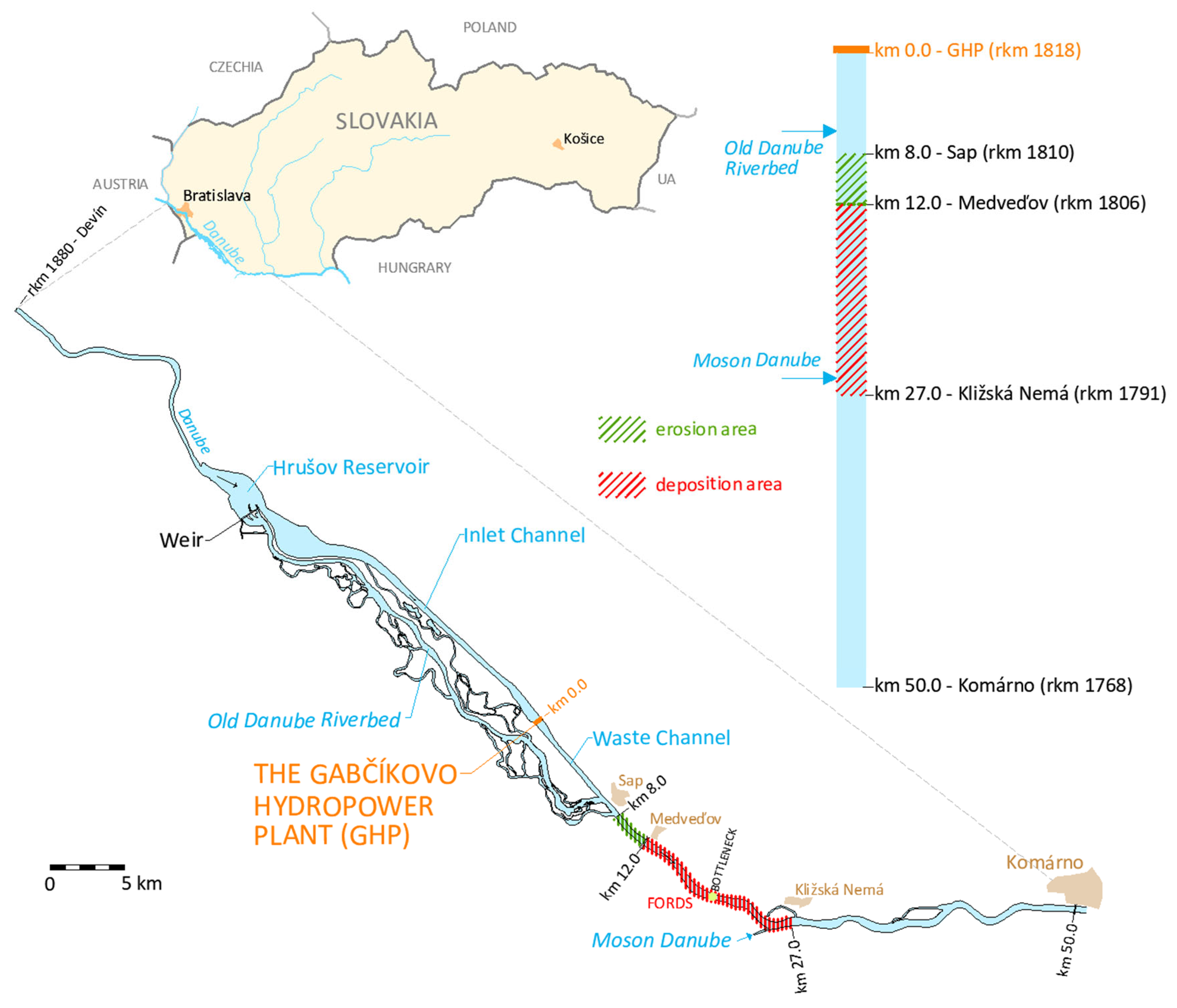
Figure 2.
Illustration of helical flow.
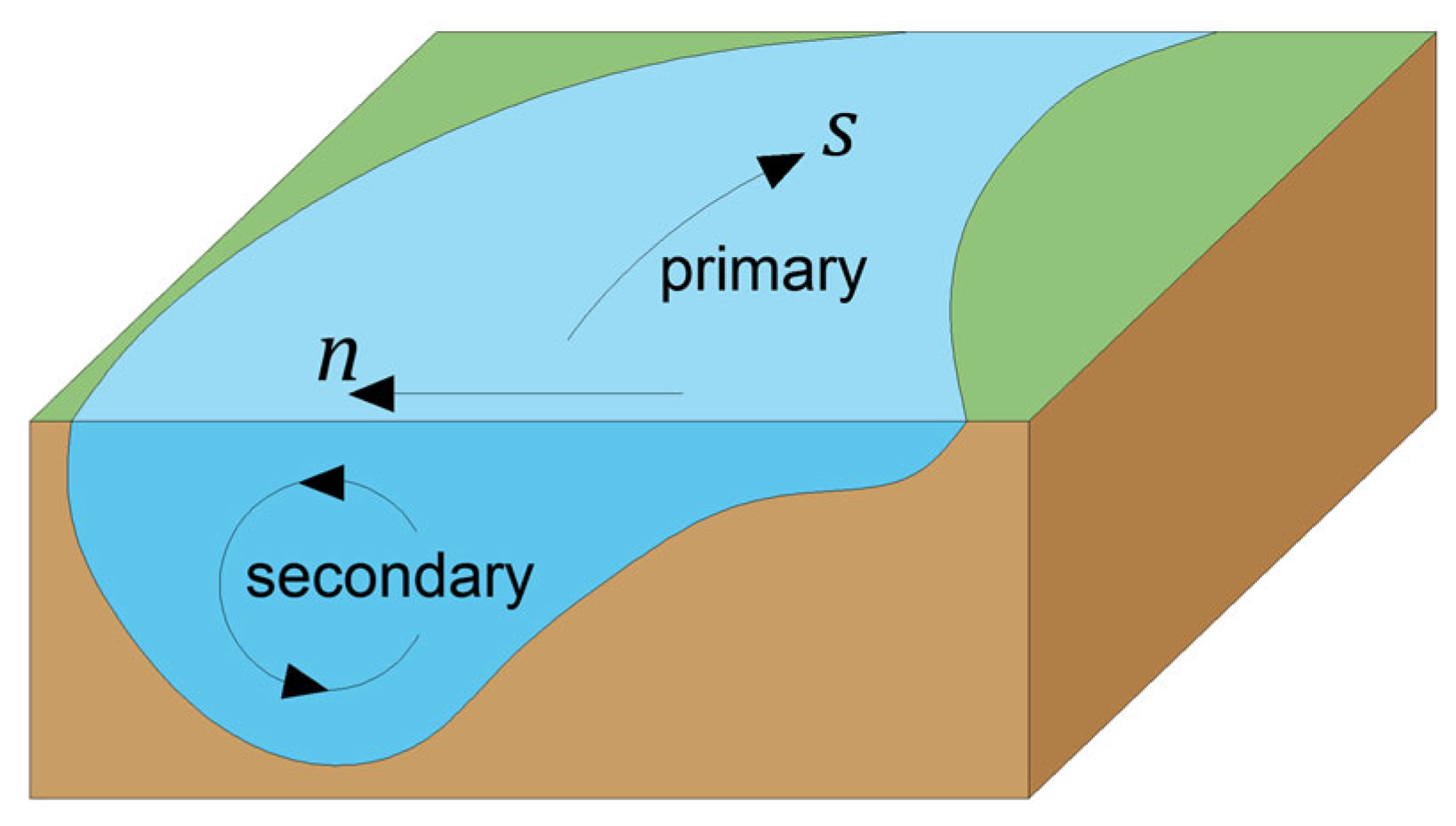
Figure 3.
Computational Scheme of the Numerical Model.
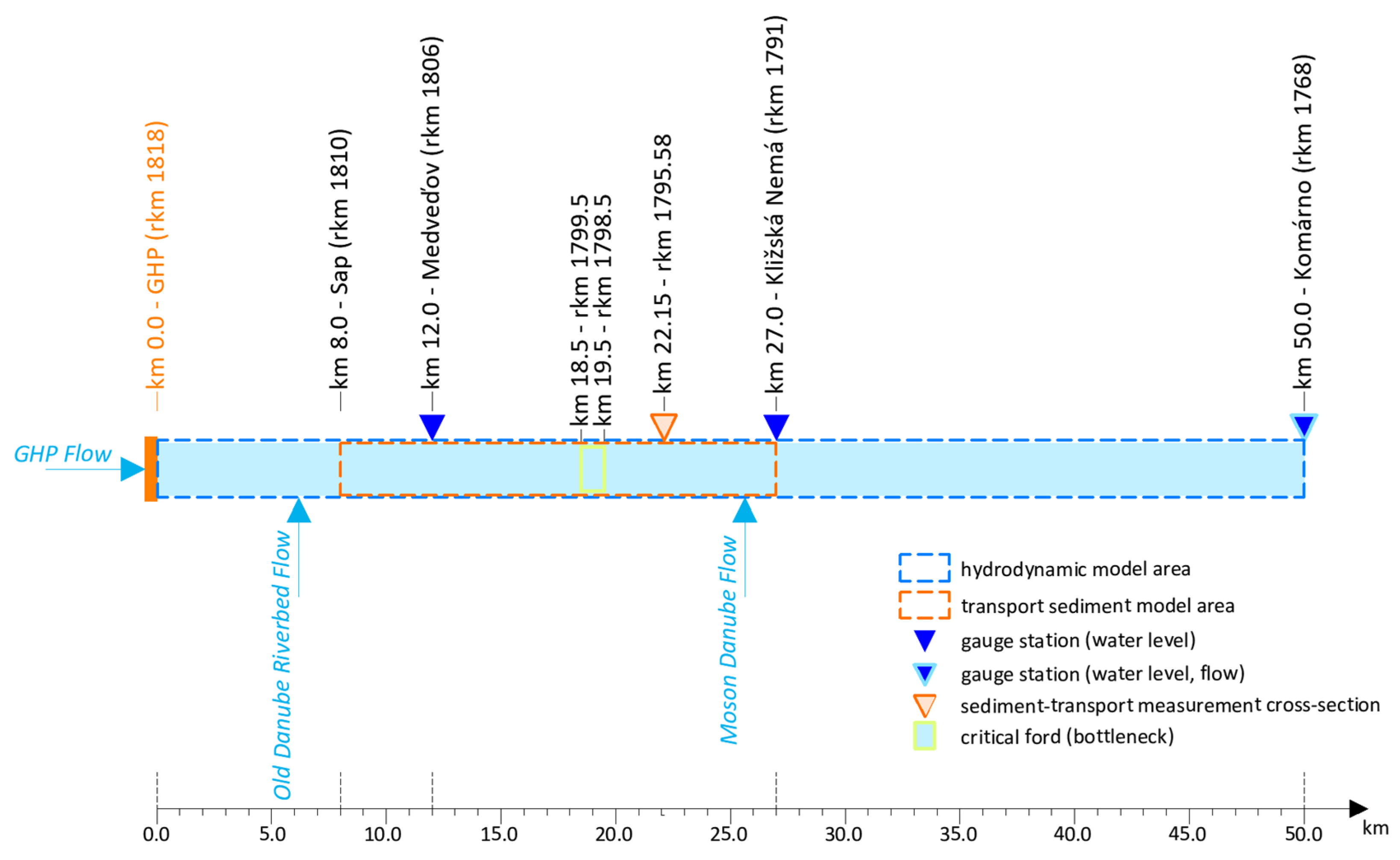
Figure 4.
Detail of the Computational Mesh.
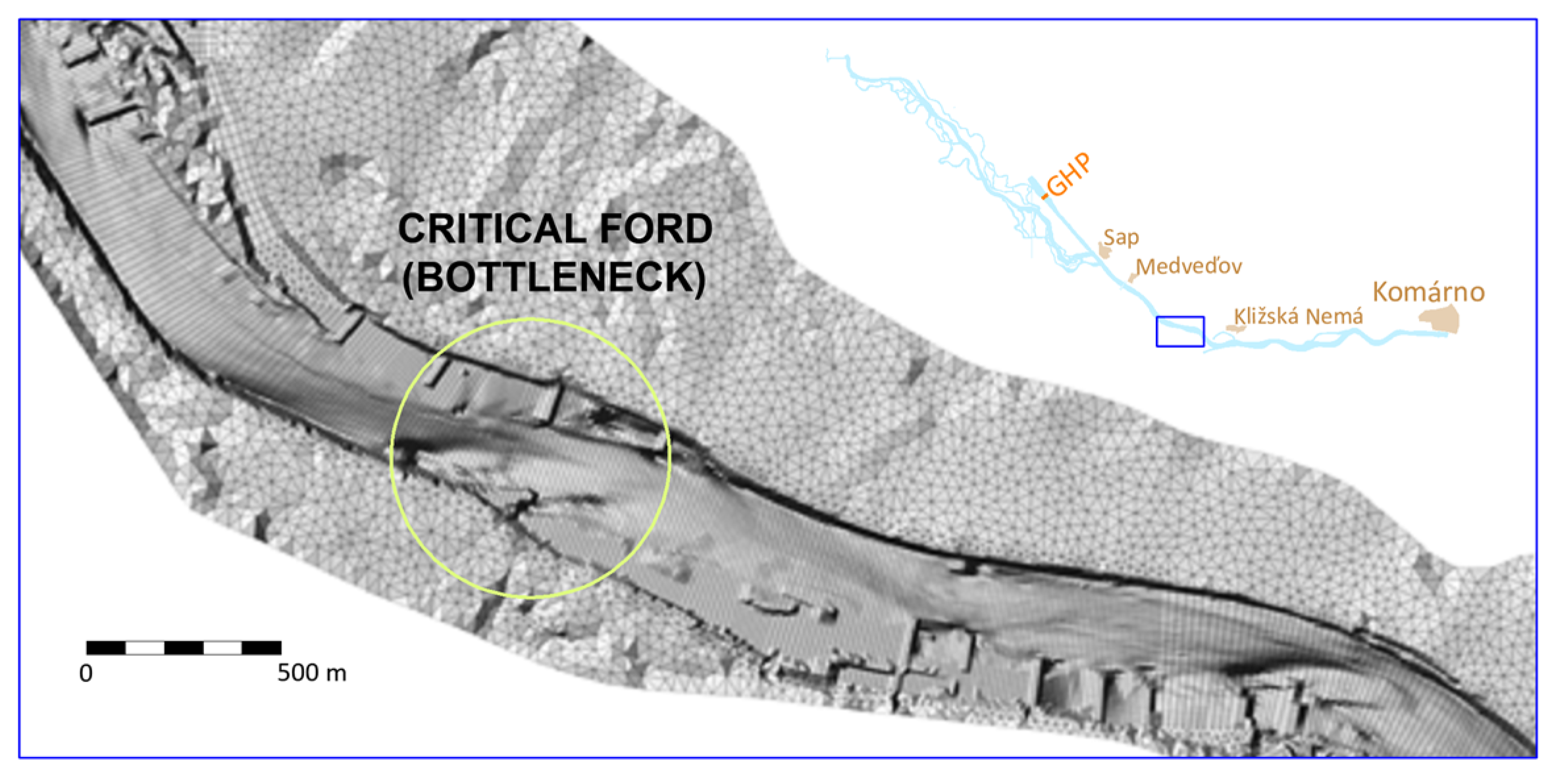
Figure 5.
The critical ford (bottleneck) at rkm 1798.5 – 1799.5 – see Figure 1, Figure 3 and Figure 4 (© Google).
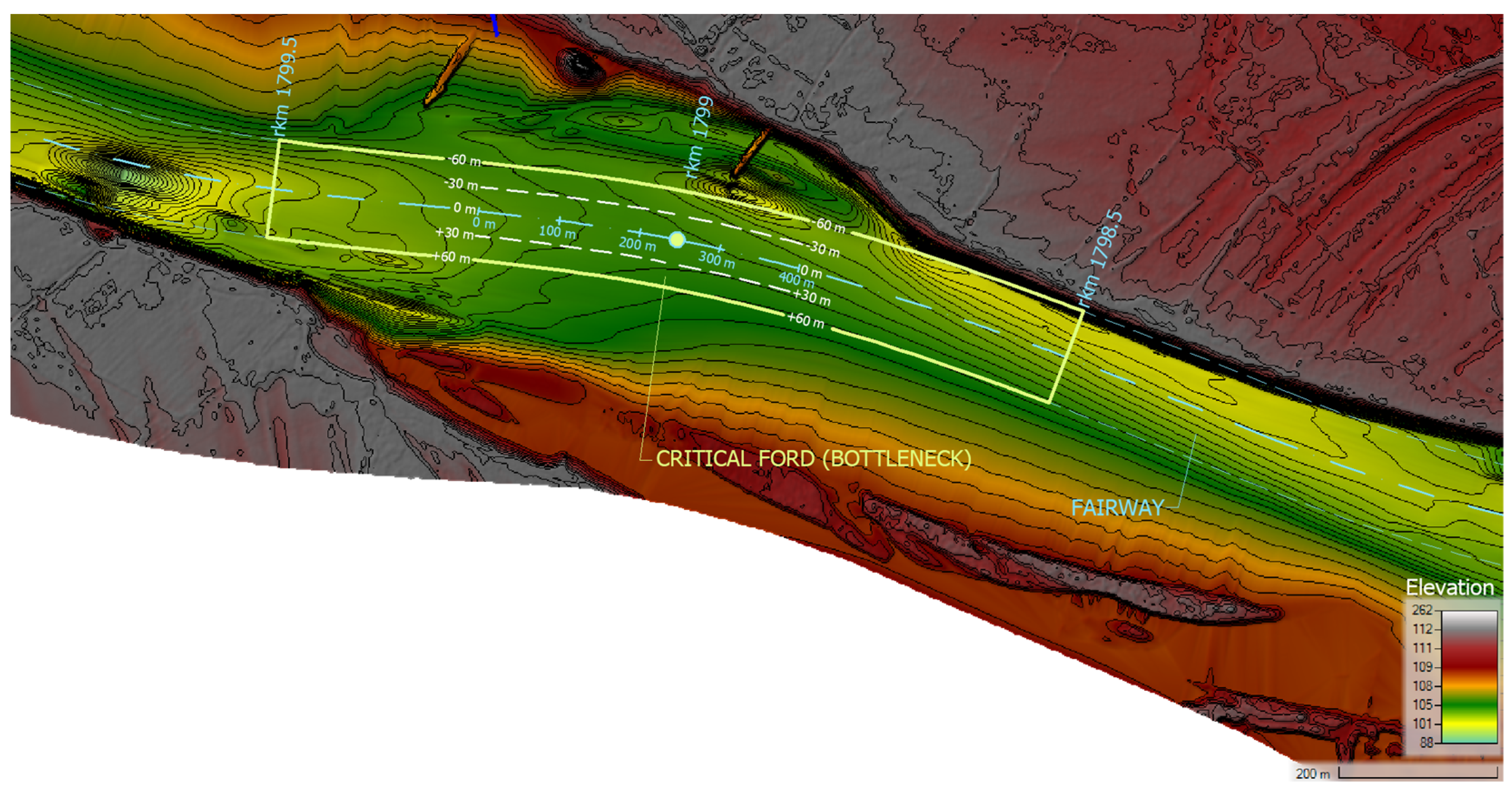
Figure 6.
Hydrographs at the GHP.
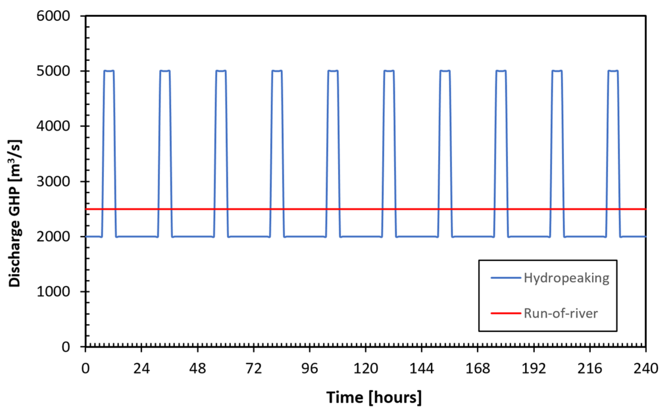
Figure 7.
Comparison of Measured and Simulated Sediment Transport Rate (Qs) at rkm 1795.58 for Different Transport Equations and Calibration Factor of Sediment Transport (kb).
Figure 7.
Comparison of Measured and Simulated Sediment Transport Rate (Qs) at rkm 1795.58 for Different Transport Equations and Calibration Factor of Sediment Transport (kb).
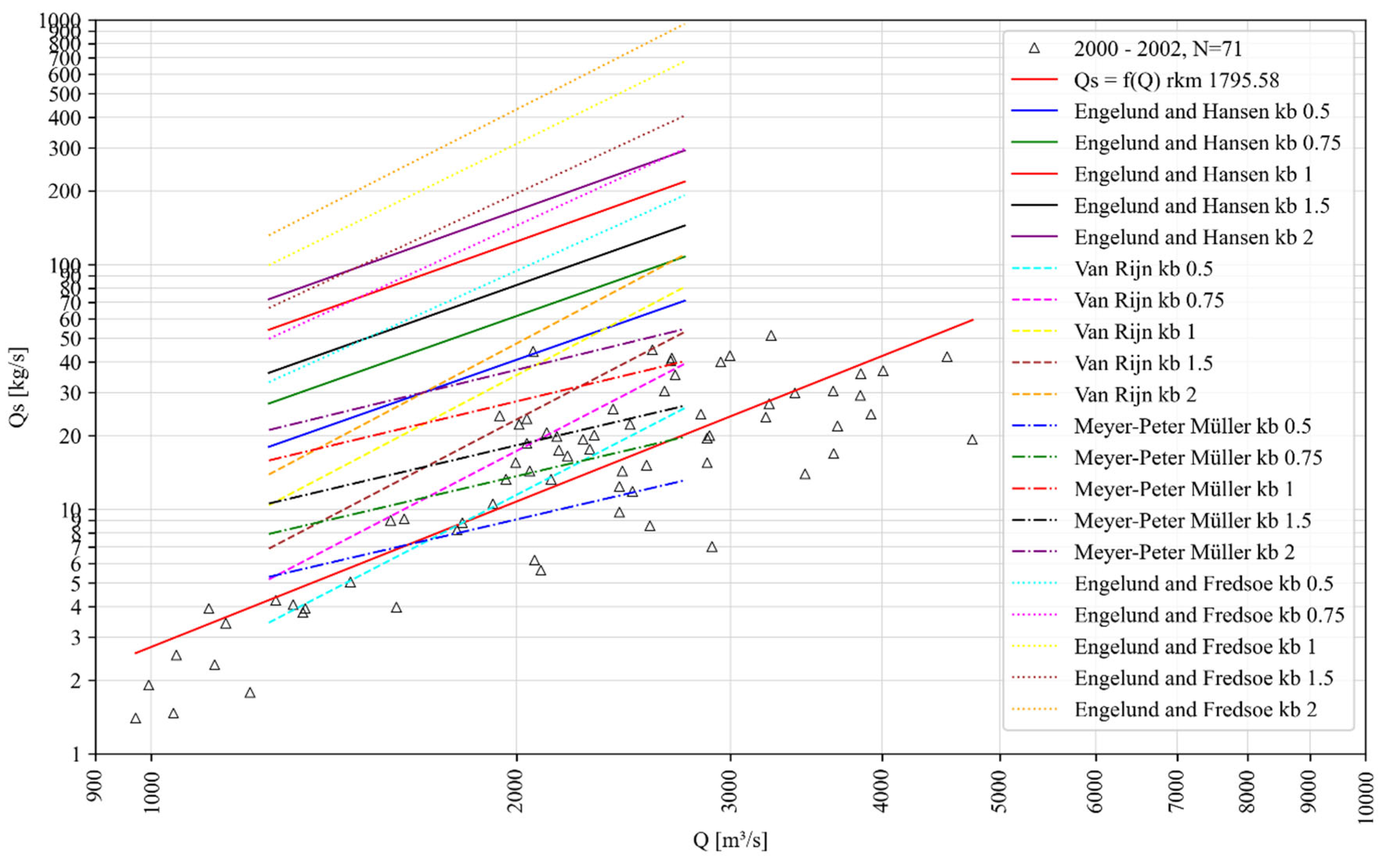
Figure 8.
Comparison of Measured and Simulated Sediment Transport Distribution at rkm 1795.58 Using the Van Rijn and Meyer-Peter Müller Sediment Transport Formula.
Figure 8.
Comparison of Measured and Simulated Sediment Transport Distribution at rkm 1795.58 Using the Van Rijn and Meyer-Peter Müller Sediment Transport Formula.
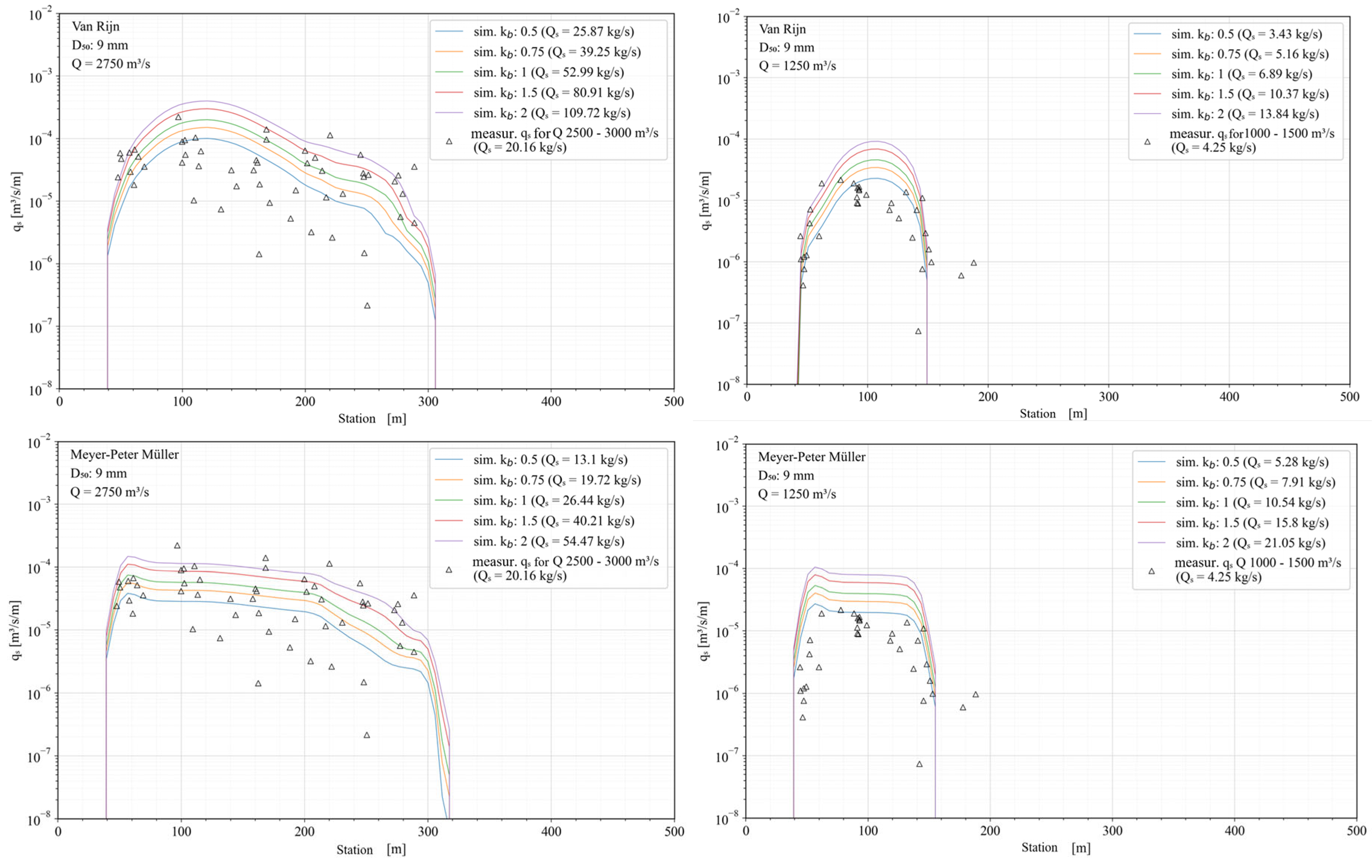
Figure 9.
Temporal development of volume of deposited sediments in the fairway at the critical ford (rkm 1798.5–1799.5).
Figure 9.
Temporal development of volume of deposited sediments in the fairway at the critical ford (rkm 1798.5–1799.5).
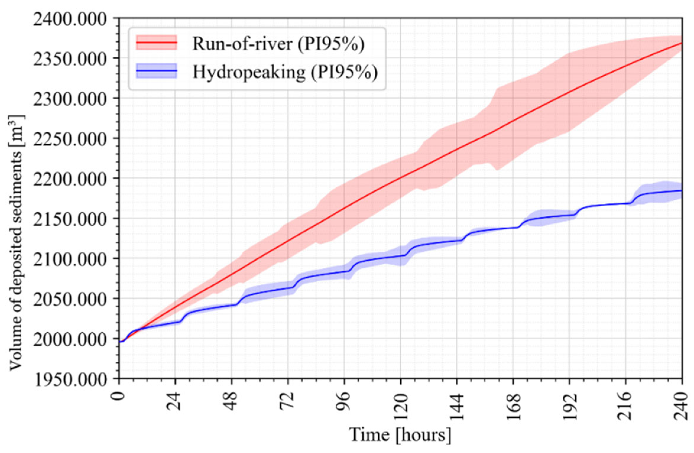
Figure 10.
Riverbed elevations at the critical ford in the monitored longitudinal profiles (as shown in Figure 5).
Figure 10.
Riverbed elevations at the critical ford in the monitored longitudinal profiles (as shown in Figure 5).
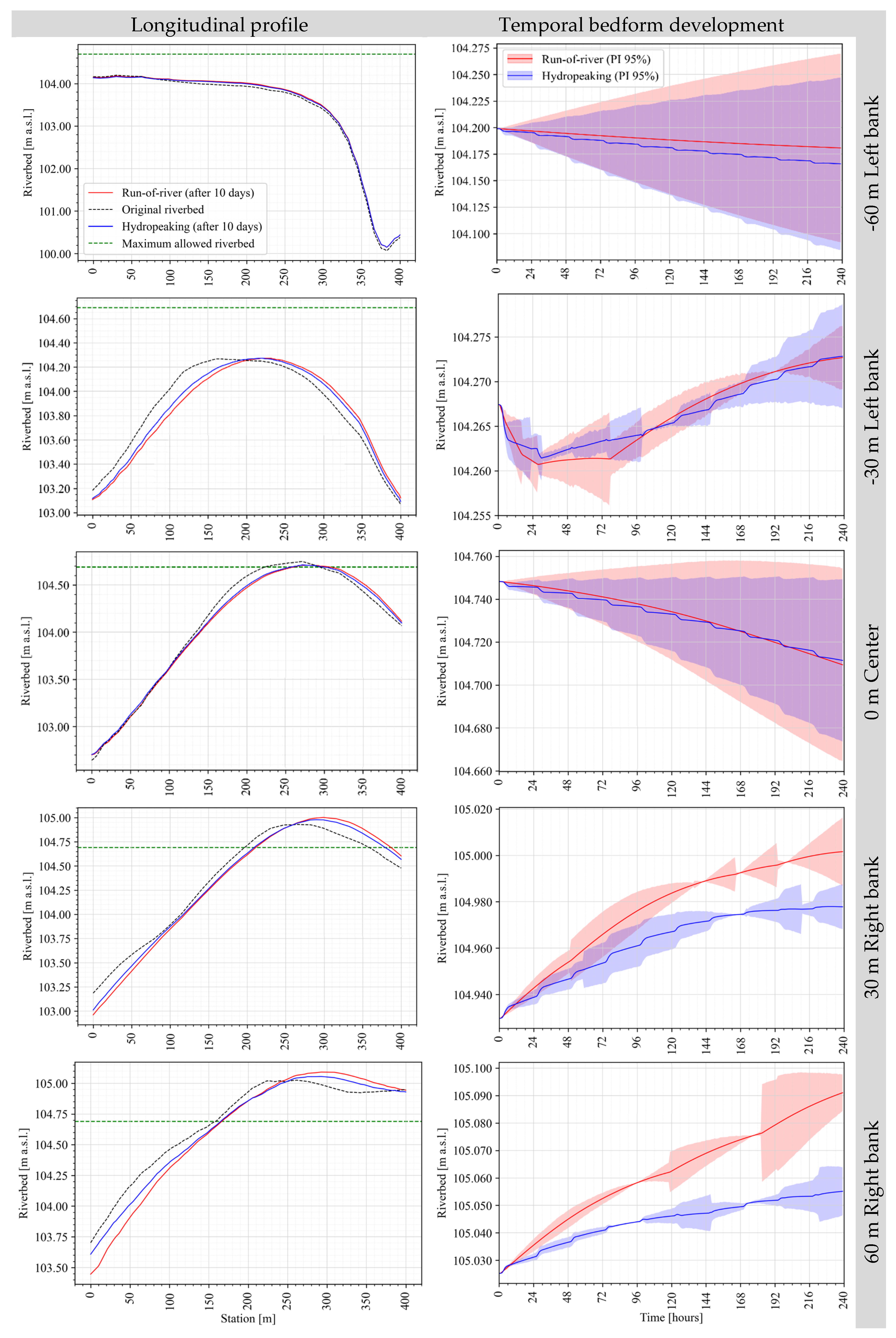
Figure 11.
Erosion and deposition areas at the critical ford after 10 days of run-of-river/ hydropeaking operation of the GHP.
Figure 11.
Erosion and deposition areas at the critical ford after 10 days of run-of-river/ hydropeaking operation of the GHP.
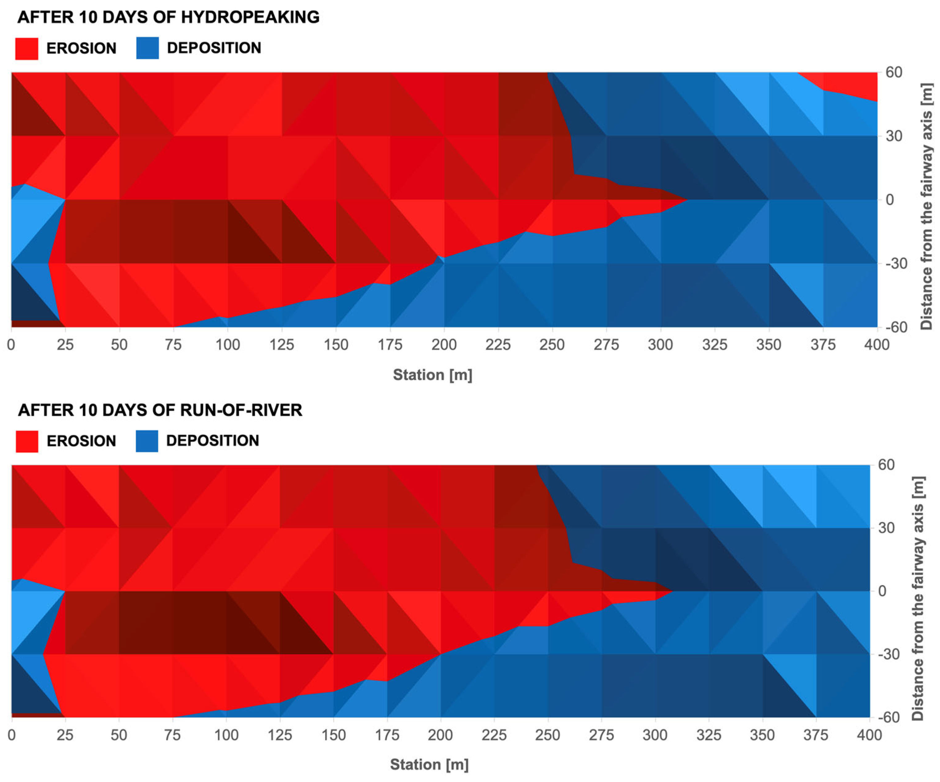

Table 1.
Hydrodynamic Model of Surface Water Flow – boundary conditions.
| Scenario | GHP Flow [m³/s] |
Flow – Old Danube Riverbed [m³/s] |
Flow - Moson Danube [m³/s] |
Water Level - Komárno [m a.s.l.] |
| 1 | 990 | 205 | 40 | 104.88 |
| 2 | 2,780 | 254 | 40 | 107.15 |
| 3 | 4,700 | 420 | 40 | 108.92 |
Table 2.
Calibration Data (measured water levels).
| Scenario | Water Level - Medveďov [m a.s.l.] |
Water Level – Kližská Nemá [m a.s.l.] |
| 1 | 108.85 | 106.18 |
| 2 | 111.65 | 108.63 |
| 3 | 113.82 | 110.74 |
Table 3.
Hydrodynamic Model Calibration.
| Scenario | Water Level - Medveďov [m a.s.l.] |
Water Level – Kližská Nemá [m a.s.l.] | RMSE | MAE | R2 | ||
| Measured | Simulated | Measured | Simulated | ||||
| 1 | 108.85 | 108.80 | 106.18 | 106.23 | 0.074 | 0.064 | 0.998 |
| 2 | 111.65 | 111.68 | 108.63 | 108.64 | |||
| 3 | 113.82 | 113.69 | 110.74 | 110.64 | |||
Table 4.
Simulated sediment transport at rkm 1795.58 with the identification of the models that best fit the observed data.
Table 4.
Simulated sediment transport at rkm 1795.58 with the identification of the models that best fit the observed data.
|
Transport formula |
kb |
Q = 2,750 m³/s QS = 20.16 kg/s |
Q = 1,250 m³/s QS = 4.25 kg/s |
RMSE | MAE | R² |
| QS [kg/s] | QS [kg/s] | |||||
| Engelund and Hansen |
0.5 | 71.08 | 17.97 | 37.29 | 32.32 | -20.95 |
| 0.75 | 107.58 | 27 | 63.87 | 55.09 | -63.42 | |
| 1 | 218.11 | 54.07 | 144.33 | 123.88 | -327.95 | |
| 1.5 | 144.17 | 36.05 | 90.53 | 77.91 | -128.4 | |
| 2 | 292.45 | 72.08 | 198.42 | 170.06 | -620.66 | |
| Engelund and Fredsoe |
0.5 | 191.95 | 33.03 | 123.17 | 100.29 | -238.54 |
| 0.75 | 297.02 | 49.67 | 198.38 | 161.14 | -620.45 | |
| 1 | 675.49 | 99.28 | 468.23 | 375.18 | -3,460.86 | |
| 1.5 | 405.51 | 66.35 | 276 | 223.73 | -1,201.81 | |
| 2 | 962.12 | 131.5 | 672.12 | 534.61 | -7,132.07 | |
| Van Rijn | 0.75 0.5 |
39.25 25.87 |
5.16 3.43 |
13.52 4.08 |
10 3.26 |
-1.88 0.74 |
| 1 | 80.91 | 10.37 | 43.17 | 33.44 | -28.43 | |
| 1.5 | 52.99 | 6.89 | 23.29 | 17.74 | -7.56 | |
| 2 | 109.72 | 13.84 | 63.69 | 49.58 | -63.05 | |
|
Meyer-Peter Müller |
1 0.5 0.75 |
40.21 13.1 19.72 |
15.8 5.28 7.91 |
16.36 5.05 2.61 |
15.8 4.05 2.05 |
-3.23 0.6 0.89 |
| 1.5 | 26.44 | 10.54 | 6.28 | 6.28 | -3.38 | |
| 2 | 54.47 | 21.05 | 27.01 | 25.55 | -10.52 |
Table 5.
The volume of deposited sediments in the fairway at the critical ford (rkm 1798.5 – 1799.5).
Table 5.
The volume of deposited sediments in the fairway at the critical ford (rkm 1798.5 – 1799.5).
| GHP Scenario | Day 0 [m3] |
After 10 days [m3] |
Δ [m3] |
After 10 days (PI95%) [m3] |
| Run-of-river (24h – 2,500 m3/s) | 1,995 | 2,368 | 373 | 2,359 – 2,377 |
| Hydropeaking (4h – 5,000 m3/s, 20h – 2,000 m3/s) | 1,995 | 2,184 | 189 | 2,174 – 2,193 |
Table 6.
Water depth in the fairway at the critical ford at the minimum navigable discharge of 1,000 m³/s.
Table 6.
Water depth in the fairway at the critical ford at the minimum navigable discharge of 1,000 m³/s.
|
Distance from the fairway’s axis [m] |
Original Depth - Day 0 - [m] |
GHP Scenario - After 10 days - |
|||
|
Run-of-river (24h – 2,500 m3/s) |
Hydropeaking (4h – 5,000 m3/s, 20h – 2,000 m3/s) |
||||
| [m] | PI 95% [m] |
[m] | PI 95% [m] |
||
| -60 | 3.20 | 3.21 | 3.12 – 3.30 | 3.22 | 3.14 – 3.31 |
| -30 | 3.13 | 3.12 | 3.11 – 3.12 | 3.12 | 3.11 – 3.12 |
| 0 | 2.65 | 2.68 | 2.64 – 2.73 | 2.68 | 2.64 – 2.72 |
| +30 | 2.46 | 2.39 | 2.37 – 2.40 | 2.41 | 2.40 – 2.42 |
| +60 | 2.37 | 2.30 | 2.29 – 2.31 | 2.34 | 2.33 – 2.34 |
*The depths represent the values of the minimum depth reached along the longitudinal profile. *The depths that are less than the threshold depth of 2.7 m are marked in red.
Table 7.
The 10-day cumulative increase/decrease of the riverbed elevation in the fairway at the critical ford.
Table 7.
The 10-day cumulative increase/decrease of the riverbed elevation in the fairway at the critical ford.
|
Distance from the fairway’s axis [m] |
GHP Scenario | ||
| Run-of-river (24h – 2,500 m3/s) | Hydropeaking (4h – 5,000 m3/s, 20h – 2,000 m3/s) | ||
| PI 95% [m] |
PI 95% [m] |
PI 95% [m] |
|
| -60 | -0.11 ~ 0.07 | -0.11 ~ 0.05 | 0.00 ~ -0.02 |
| -30 | 0.00 ~ 0.01 | 0.00 ~ 0.01 | 0.00 ~ 0.00 |
| 0 | -0.08 ~ 0.01 | -0.07 ~ 0.00 | 0.01 ~ -0.01 |
| +30 | 0.06 ~ 0.09 | 0.04 ~ 0.06 | -0.02 ~ -0.03 |
| +60 | 0.06 ~ 0.07 | 0.02 ~ 0.04 | -0.04 ~ -0.03 |
Disclaimer/Publisher’s Note: The statements, opinions and data contained in all publications are solely those of the individual author(s) and contributor(s) and not of MDPI and/or the editor(s). MDPI and/or the editor(s) disclaim responsibility for any injury to people or property resulting from any ideas, methods, instructions or products referred to in the content. |
© 2026 by the authors. Licensee MDPI, Basel, Switzerland. This article is an open access article distributed under the terms and conditions of the Creative Commons Attribution (CC BY) license (http://creativecommons.org/licenses/by/4.0/).
Copyright: This open access article is published under a Creative Commons CC BY 4.0 license, which permit the free download, distribution, and reuse, provided that the author and preprint are cited in any reuse.


