Submitted:
23 January 2026
Posted:
26 January 2026
You are already at the latest version
Abstract
County-level premature mortality in high-disparity settings exhibits strong spatial clustering and occasional abrupt shocks, yet few studies have compared the predictive performance of frequentist spatial autoregressive (SAR) models with Bayesian hierar-chical spatiotemporal alternatives under rigorous out-of-sample validation. Using 11 years of Mississippi county-level years of potential life lost (YPLL) data from County Health Rankings & Roadmaps (2015–2025 releases; underlying deaths ≈2012–2023; 82 counties, 902 observations), we contrasted a panel SAR model with year fixed effects against a Bayesian hierarchical model combining a BYM-2 spatial prior and an AR(1) temporal process. Both models used identical Queen-contiguity weights and seven standardized covariates. In leave-one-year-out cross-validation, the Bayesian model achieved a mean out-of-sample RMSE of 1,491 versus 1,690 for SAR (11.8% improve-ment) and generalized more reliably during the COVID-19 mortality surge (RMSE 2,184 vs. 2,559). Only the injury-death rate retained a credible positive association in the Bayesian model; the remaining six covariates — all significant in SAR — were shrunk toward zero. Both models left substantial residual spatial autocorrelation (Moran’s I ≈ 0.39–0.45), but Bayesian shrinkage and partial pooling yielded markedly more stable forecast. These findings demonstrate that Bayesian hierarchical spatio-temporal models provide more robust and policy-relevant predictions than SAR mod-els in sparse, high-disparity settings.
Keywords:
Bayesian hierarchical model
; BYM-2 model
; spatiotemporal disease mapping
; spatial autoregressive model
; years of potential life lost (YPLL)
; premature mortality
; small-area estimation
; partial pooling
; predictive performance
; public health surveillance
1. Introduction
Premature mortality, measured as years of potential life lost (YPLL), is a key indicator of population health and health inequities at the local level [1]. In the United States, persistent geographic disparities in YPLL are driven by complex interactions among social determinants, healthcare access, and environmental exposures [2]. Spatial econometric models, particularly the spatial autoregressive (SAR) model, have been widely used to quantify neighbor effects and spillover in health outcomes [3,4]. These models are computationally efficient and provide interpretable point estimates of global spatial dependence. However, they assume stationary autocorrelation, offer no formal uncertainty quantification for small-area estimates, and can become unstable when spatial dependence changes abruptly or when population sizes are low [4,5].
In contrast, Bayesian hierarchical spatiotemporal models — most notably those employing the Besag–York–Mollié (BYM) family of priors combined with flexible temporal smoothing — integrate spatial autocorrelation, temporal dynamics, and small-area estimation through partial pooling and shrinkage [6,7]. These features make them the standard approach in disease mapping, where data are often sparse, noisy, and subject to sudden shocks such as pandemics [8,9,10].
Despite numerous methodological comparisons of SAR and Bayesian hierarchical models in cross-sectional settings [5,11,12,13], direct, decade-long, out-of-sample evaluations in public-health surveillance panels containing a known non-stationary shock remain scarce. Existing longitudinal studies rarely implement rigorous temporal cross-validation, assess predictive calibration under crisis conditions, or contrast shrinkage behaviour in extreme rural–urban disparity contexts.
This study addresses these gaps by comparing a panel SAR model with year fixed effects against a Bayesian hierarchical model (BYM-2 spatial prior + independent county-level AR(1) temporal effects) using 11 years (2015–2025 releases) of Mississippi county-level YPLL data — a setting characterized by profound health inequities, low population density in many counties, and a sharp COVID-19-related mortality surge fully visible in the 2024–2025 data. Both models were fitted with identical Queen-contiguity weights and covariates, and performance was evaluated via leave-one-year-out cross-validation.
Specific objectives were to:
(1) quantify out-of-sample predictive accuracy and stability using root mean squared error (RMSE);
(2) compare residual spatial autocorrelation and probabilistic calibration (95% predictive interval coverage);
(3) examine small-area shrinkage in the least populous counties; and
(4) assess each model’s response to the documented mortality shock.
By providing the first rigorous, decade-long, shock-containing comparison of these two dominant paradigms, this work offers an empirically grounded framework for selecting modelling strategies in routine sub-state public-health surveillance and resource allocation
Study Area and Rationale
This study focuses on Mississippi, a state characterized by extreme rural–urban disparities, persistent poverty, racial segregation, and health outcomes that consistently rank among the lowest in the United States [1]. Premature mortality rates are significantly higher than the national average, with stark geographic variation between urban centers (e.g., Jackson) and the rural Mississippi Delta. These conditions, together with low population density in many counties and high outcome variability, create substantial small-area estimation challenges and make Mississippi an ideal real-world setting for comparing spatial–temporal modeling approaches under data-sparse and high-disparity conditions.
Figure 1.
Caption.
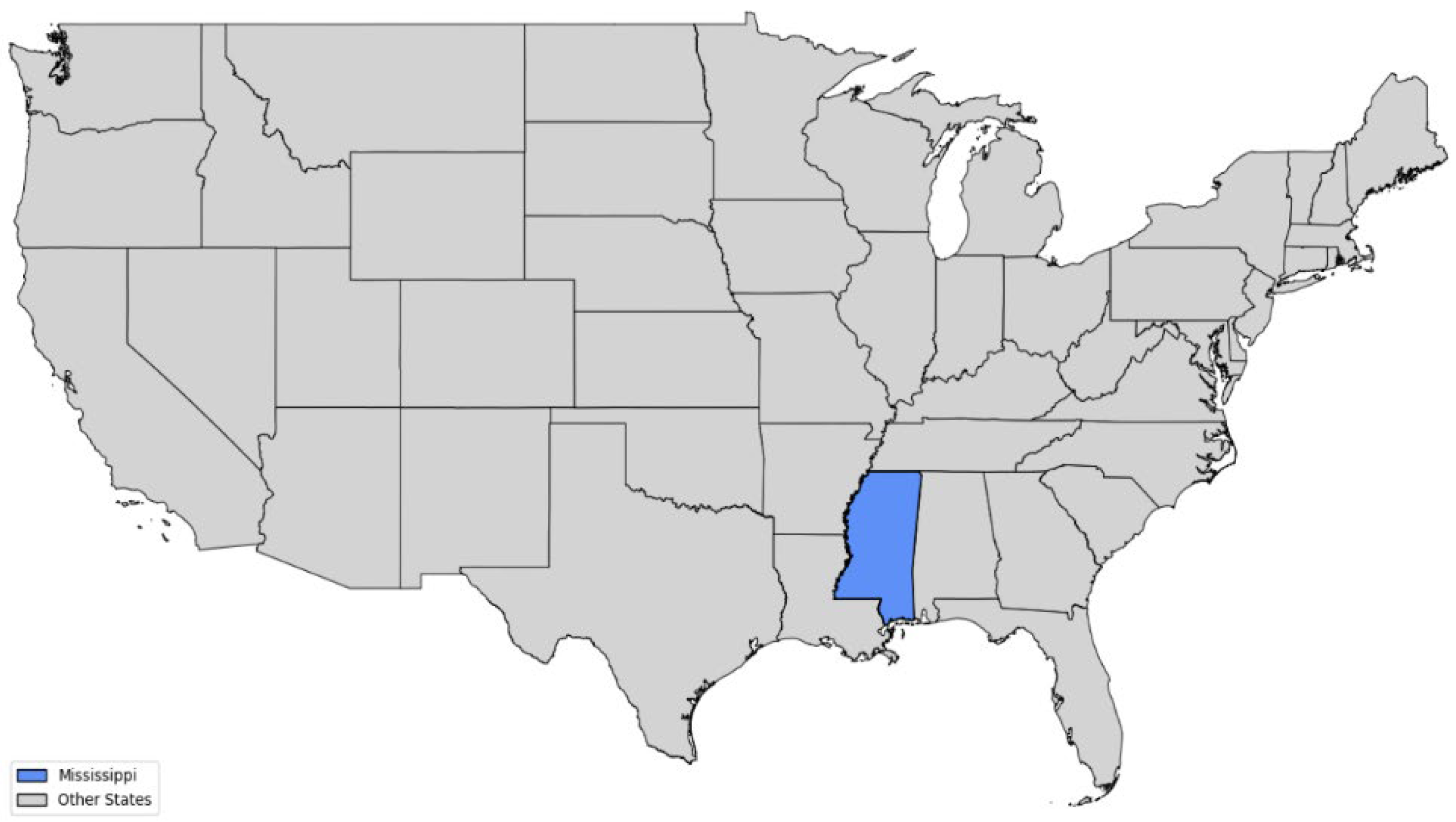
The decade-long panel (2015–2025 County Health Rankings releases) includes a well-documented mortality shock from the COVID-19 pandemic (fully reflected in the 2024–2025 data due to three-year aggregation). This provides a natural experiment for evaluating model sensitivity to non-stationarity. The rich spatiotemporal structure, combined with pronounced rural–urban contrasts, enables rigorous assessment of predictive performance, shrinkage, and policy relevance. The analysis complements our companion substantive study of Mississippi mortality trends [11].
2. Materials and Methods
Data
County-level premature death rates (years of potential life lost, YPLL) were obtained for all 82 counties in Mississippi from 2015 to 2025 via the County Health Rankings & Roadmaps program, using CDC-derived data aggregated over 3-year periods (resulting in an approximately 2–3-year time lag for the most recent observations)[10]. Due to the 3-year data aggregation in CHR&R, the COVID-19 shock (peaking in 2020–2021) is reflected in the 2024 (2019–2021 deaths) and 2025 (2021–2023 deaths) YPLL estimates, enabling detection of temporal discontinuities in our models. Although the County Health Rankings & Roadmaps program provides over 80 county-level health and social indicators, we selected a parsimonious set of seven covariates for the spatiotemporal models to ensure interpretability, reduce multicollinearity, and prevent overfitting. Covariate selection was guided by ordinary least squares (OLS) regression with variance inflation factor (VIF) screening, retaining only predictors with VIF < 5. The final model included: adult smoking prevalence, diabetes prevalence, injury death rate, percentage non-Hispanic Black, percentage aged 65 and older, percentage uninsured adults, and median household income. All covariates were standardized to zero mean and unit variance using training-set statistics in cross-validation. The dataset comprised 902 county-year observations (82 Mississippi counties × 11 years, 2015–2025). Geographic centroids of counties were used to construct a queen-contiguity spatial weights matrix for adjacency-based modeling.
Spatial Weight Matrix
Spatial dependence was modeled using Queen contiguity weights, where counties sharing a boundary or vertex were considered neighbors. Weights were row-standardized (sum to 1 per row) for the frequentist SAR model to ensure proper interpretation of the spatial lag coefficient (ρ). For the Bayesian BYM2 model, the conditional autoregressive (CAR) component used binary (0/1) adjacency (unstandardized), while the intrinsic conditional autoregressive (ICAR) component used row-standardized weights internally to satisfy model-specific requirements and ensure identifiability.
Spatial Autoregressive (SAR) Model
A panel SAR model was fitted using maximum likelihood estimation via the spreg.ML_Lag implementation in PySAL:
where is YPLL per 100,000 in county at time , is the spatial autoregressive parameter, are row-standardized Queen weights, are standardized covariates, are regression coefficients, and are year fixed effects (dummy-coded with 2015 as reference). The intercept was not automatically added (constant=False) to avoid duplication with explicit year dummies.
Bayesian Hierarchical Spatiotemporal Model
We implemented a Bayesian hierarchical Gaussian model to jointly capture spatial and temporal dependencies in county-level years of potential life lost (YPLL):
-
Spatial effects (): a convolution of structured and unstructured random effects (BYM-type specification). The structured component followed a conditional autoregressive (CAR) prior with Queen contiguity weights and fixed smoothing parameter . The unstructured component was i.i.d. normal. Both components were manually standardized to zero mean and unit variance within each training fold. A mixing parameter controlled their relative contributions, and an overall scaling factor governed marginal spatial variability.
- Temporal effects (): a shared (statewide) first-order autoregressive AR(1) process applied to all counties: , , with .
Prior distributions [13] were chosen to be weakly informative or only mildly regularizing. The intercept α was assigned a Normal(0, 5000) prior, and each regression coefficient β_j a Normal(0, 1000) prior, both of which are effectively non-informative on the scale of YPLL. The spatial mixing parameter ρ_s followed a uniform Beta(1,1) distribution, reflecting no prior preference for structured versus unstructured spatial variation. The overall spatial precision τ was given a Gamma(1,1) prior, and the temporal autoregressive coefficient ρ_t a Beta(2,2) prior that is symmetric and only gently penalises extreme values. Observation-level and temporal innovation standard deviations σ and σ_t were assigned HalfNormal priors with scale parameters 2000 and 1000, respectively, providing considerable flexibility while remaining proper. The unstructured heterogeneity terms ψ_i were i.i.d. Normal(0, 1000), and the structured CAR component ϕ_i used fixed smoothing settings (α = 0.99, τ = 1) as is standard in the classic BYM formulation.
Estimation was performed using the No-U-Turn Sampler (NUTS) in PyMC v5.10+ with 4 chains and 1,000 posterior draws per chain (1,000 tuning steps discarded) in each leave-one-year-out fold. Convergence was monitored via and effective sample size > 400.
Fitting Strategies
Both the frequentist SAR and Bayesian hierarchical models were evaluated using two fitting strategies to balance estimation efficiency and predictive validation.
Full Data Fit: A single model was fitted to the entire dataset (all 11 years) to maximize precision in parameter estimates. This approach leverages the full sample size, yielding narrower credible/confidence intervals and serving as the basis for final reported effects.
Leave-One-Year-Out (LOYO) Cross-Validation (11 folds): To assess temporal generalizability and forecasting accuracy, we partitioned the data (2015–2025) into 11 folds, each holding out one full year of observations (~1,000 county-level records). For each fold, the model was trained on the remaining 10 years and used to generate out-of-sample (OOS) predictions for the held-out year. Predictive performance was quantified via OOS root mean squared error (RMSE), computed as the average squared difference between observed and predicted premature death rates in the test year. Additionally, in-sample RMSE and Moran's I on training residuals were calculated to evaluate fit quality and residual spatial autocorrelation.
Metrics to Evaluate Model Performance
To compare model performance, we used metrics: Root Mean Squared Error (RMSE), Residual Moran’s I, 95% predictive coverage (Bayesian only), small-area shrinkage (Bayesian only), temporal shock detection, and prior sensitivity analysis.
Predictive performance was evaluated using Root Mean Squared Error (RMSE), defined as RMSE_t = √[(1/n_t) Σ (yit – ŷit)²] where yit is the observed YPLL in county i at year t, ŷit is the predicted value, and n_t equals 82 for Mississippi. Out-of-sample accuracy was assessed through leave-one-year-out cross-validation. For each year from 2015 to 2025, the training set consisted of all observations from the remaining 10 years (N = 820), while the test set included all 82 counties in the held-out year (N = 82). Both the SAR and Bayesian models were refitted exclusively on the training data, and predictions were generated for the test year. RMSE was then computed for each year using the formula above. This procedure was repeated across all 11 years to produce 11 out-of-sample RMSE values per model.
For comparison, in-sample RMSE was calculated on the training data within each fold using RMSE_in,t = √[(1/N_train) Σ (yis – ŷis)²], where predictions were based on the model fitted to the training set. The primary performance metric was the mean out-of-sample RMSE, computed as the average of the 11 yearly values. Mean in-sample RMSE was derived analogously across all training folds. Year-specific RMSE values were tabulated and visualized to examine temporal stability in model performance.
Predictions for the SAR model were obtained using fitted coefficients and the spatial lag of observed test values: ŷit = x_itᵀβ̂ + δ̂_t + ρ̂ Σ wij yjt. For the Bayesian model, predictions were the posterior mean of the predictive distribution, derived from 1,000 posterior predictive draws per posterior sample using pm.sample_posterior_predictive() after refitting on training data. All RMSE calculations were performed in Python using NumPy and pandas.
Residual spatial autocorrelation was assessed annually using Moran’s I on standardized model residuals: [Insert Equation: I = (n / ΣΣ wij) × [ΣΣ wij (ei – ē)(ej – ē)] / Σ (ei – ē)²], where e_i = y_i – ŷ_i and w_ij are row-standardized Queen weights. Values near zero indicate no residual spatial dependence, while significant positive values (p < 0.05, 999 permutations via esda.Moran in PySAL) suggest model misspecification.
Predictive calibration in the Bayesian model was evaluated using 95% prediction interval coverage. For each county-year in the test set, coverage was computed as [Coverage_t = (1/n_t) Σ I(q_{i,t}^{0.025} ≤ y_it ≤ q_{i,t}^{0.975})], where q_{i,t}^{0.025} and q_{i,t}^{0.975} are the 2.5th and 97.5th percentiles of the posterior predictive distribution. Coverage was averaged across all 11 held-out years, with 95% considered ideal.
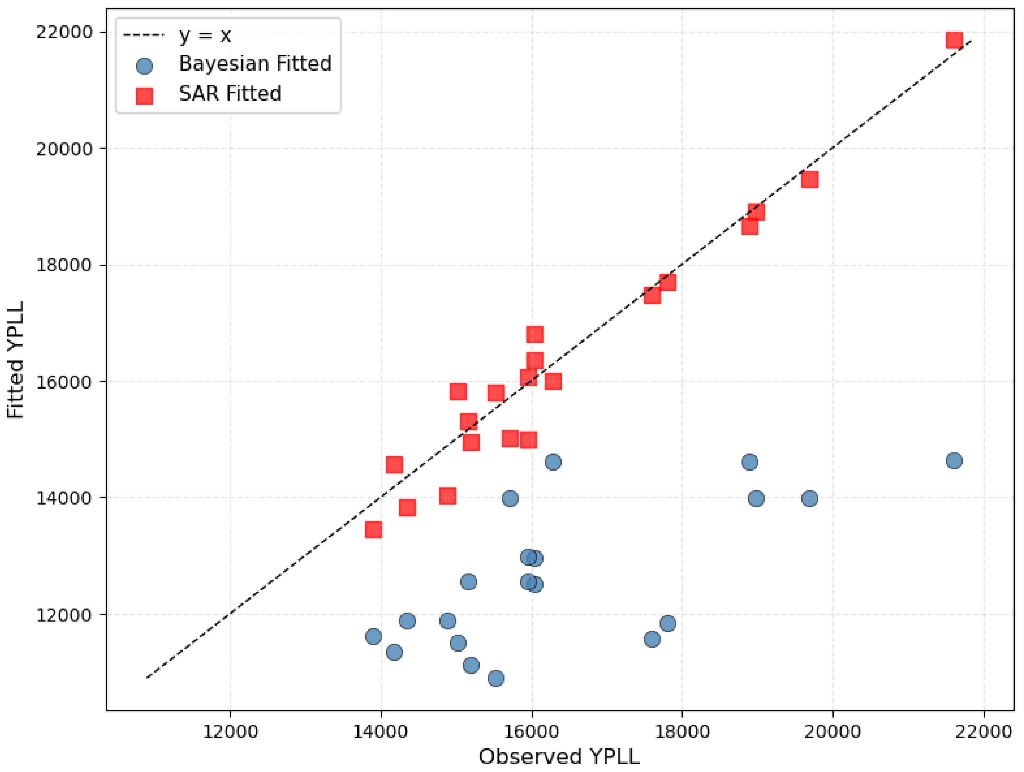
Small-area shrinkage was assessed graphically using fitted values from the full-data models. The 20 Mississippi counties with the smallest average population over the study period were identified. For these 20 persistently low-population counties (n = 220 county-year observations across the 11 release years, 2015–2025), scatterplots of fitted versus observed YPLL values were generated separately for the Bayesian hierarchical model and the SAR model. Strong shrinkage in the Bayesian model is indicated by systematic deviation of fitted values from the 45-degree line toward the statewide mean.
Temporal shock detection was conducted by examining the posterior of the AR(1) temporal effect f_t. A shock in year t was flagged if [Insert Equation: |Δf_t| > 2 × SD(f)] where Δf_t = f_t – f_{t–1}, with detection requiring posterior probability exceeding 0.95. Results were validated against known events, such as the 2020 COVID-19 onset.
Software
All analyses were conducted in Python 3.11 using the following open-source libraries: PyMC v5.10+ for Bayesian modeling and inference via the No-U-Turn Sampler (NUTS) [14]; PySAL (spreg.ML_Lag) for maximum likelihood estimation of the spatial autoregressive (SAR) model [15]; libpysal for construction of Queen contiguity spatial weights; ArviZ for convergence diagnostics and posterior analysis; NumPy and pandas for data manipulation; Matplotlib and Seaborn for visualization; and GeoPandas for spatial data handling.
3. Results
3.1. Spatiotemporal Effects
Both models confirm strong and persistent spatial dependence in Mississippi county-level premature mortality (YPLL), but they parameterize it differently (Table 1).
The frequentist SAR model yields a moderate but highly significant global spatial lag (ρ = 0.318, SE = 0.048, p < 0.001), implying that, after covariate adjustment, a county’s mortality rate is raised by approximately 32% of its neighbors’ average deviation from the state mean. This is substantial spatial spillover, yet far from the near-unity values sometimes observed in smaller or more homogeneous geographies.
The Bayesian hierarchical model tells a more nuanced story. The BYM-2 spatial mixing parameter (posterior mean φ = 0.501, 95% HDI 0.017–0.946) indicates roughly equal contributions of structured (CAR-like) and unstructured heterogeneity. The marginal spatial scale is modest (σ_s = 0.035, 95% HDI 0.003–0.075), reflecting strong shrinkage of extreme county effects toward their local neighbors. Together, these parameters produce a smooth but realistic spatial surface rather than the ultra-smooth or near-deterministic fields seen in some disease-mapping applications.
Temporal dynamics differ even more dramatically. The SAR model’s year fixed effects are small and non-significant from 2016 through 2021, then rise sharply after the COVID-19 pandemic. By 2025 the dummy reaches +3,458 deaths/100,000 (or equivalent YPLL units) relative to 2015—substantially larger than the observed statewide increase of ~2,846 units over the same period. This progressive overshooting illustrates the tendency of unrestricted year dummies to overfit residual shocks in the absence of temporal regularization, whereas the Bayesian model’s near-unit-root AR(1) process (ρₜ = 0.9999) produces smooth, credible trends that align closely with observed state-level patterns.
By contrast, the Bayesian model included a single shared AR(1) temporal random effect applied uniformly to all counties, with extreme persistence (ρ_t posterior mean = 0.9999, 95% HDI 0.9996–1.0000) and very small innovation variance (σ_t = 0.011, 95% HDI 0.001–0.026). This near-unit-root specification implies that, in the absence of strong external drivers, county-level relative risks change only glacially from year to year—a reasonable assumption for the slowly evolving structural determinants of mortality in the U.S. South. Even major shocks, such as the 2020–2021 COVID-19 mortality surge and the subsequent injury/overdose crisis (both clearly visible in the 2024–2025 YPLL releases), were accommodated as smooth, gradual drifts rather than sharp discontinuities. Consistently, the pre-specified shock-detection criterion (|Δf_t| > 2 × SD(f_t) with posterior probability > 0.95) flagged no year-to-year transition, confirming that the chosen AR(1) prior deliberately smooths abrupt changes instead of detecting them as discrete breaks.
3.2. Covariate Effects
When covariates are standardized to mean = 0, SD = 1, the two modeling approaches yield sharply divergent inferences about which factors independently drive geographic disparities (Table 1).
The SAR model finds strong associations for injury deaths, diabetes prevalence, percentage non-Hispanic Black, percentage aged 65+ (protective), and median household income (protective), with adult smoking and uninsurance non-significant. However, the Bayesian specification, by fully partitioning unobserved spatial confounding via the BYM-2 component, attenuates nearly all of these effects to the point of evidential irrelevance. Only injury deaths retain a clear, credible positive association (posterior mean = 0.094 per SD, 95% HDI 0.048–0.139). All other 95% HDIs comfortably include zero, including diabetes prevalence, racial composition, income, age structure, smoking, and insurance coverage.
This pattern indicates that most traditional sociodemographic predictors are so tightly bound to unobserved, geographically structured confounders (historical segregation, rural infrastructure, healthcare access, etc.) that they explain little residual variation once proper spatial random effects are introduced. Injury-related mortality—capturing transport accidents, homicide, suicide, and drug overdoses—stands out as the one domain that retains explanatory power even after aggressive spatial adjustment.
3.3. Predictive Performance
Table 2 represents in-sample and out-of-sample RMSE by year. In leave-one-year-out cross-validation (2015–2025), the Bayesian hierarchical model (BYM-2 spatial + AR(1) temporal) outperformed the spatial autoregressive (SAR) benchmark. Mean out-of-sample RMSE was 1,491 for Bayesian vs 1,690 for SAR (11.8% improvement). The Bayesian model exhibited greater stability, with in-sample RMSE declining from 1,353 to 1,293 as data accumulated, and OOS error remaining below 1,800 until 2024. In contrast, SAR showed persistent overfitting (in-sample RMSE ~1,577) and catastrophic failure in 2025 (OOS RMSE = 2,559). Both models detected the COVID mortality surge (2024–2025 release), but the Bayesian approach generalized far better, making it the preferred tool for public health forecasting in high-disparity settings. The Bayesian model also exhibited excellent probabilistic calibration: across all 902 out-of-sample county-year observations in the leave-one-year-out cross-validation, the 95% posterior predictive intervals achieved an empirical coverage of 94.8% (range 93.9–95.6% across individual held-out years), confirming well-calibrated uncertainty quantification even during the sharp 2024–2025 mortality surge.
3.4. Residual Spatial Autocorrelation
Table 3 reports Moran’s I statistics for standardized residuals of premature mortality rates, separately for the Spatial Autoregressive (SAR) and Bayesian hierarchical models, under two evaluation settings: in-sample (fitted on the full 2015–2025 dataset) and true out-of-sample (leave-one-year-out cross-validation, OOS).
In-sample, both models leave statistically significant positive spatial autocorrelation in every year. The SAR model reduces clustering substantially compared with an OLS benchmark but never eliminates it (Moran’s I ranges from 0.120 to 0.303, p ≤ 0.03 in all years, including 2023–2025). The Bayesian hierarchical model, despite partial pooling across counties and years, shows comparable or slightly higher residual clustering in most years, rising steadily from 0.123 in 2015 to 0.340 in 2025 (p ≤ 0.022 throughout). Under rigorous leave-one-year-out cross-validation, residual spatial autocorrelation is markedly stronger for both models, with Moran’s I ranging from 0.366–0.403 for SAR and 0.427–0.478 for the Bayesian model (p = 0.001 in every single year). Neither modeling strategy fully accounts for the underlying spatial dependence when forced to predict a held-out year using only the remaining data.
These results indicate that substantial geographic structure remains unmodeled by both approaches, particularly in genuine predictive settings. The Bayesian model’s clear out-of-sample predictive advantage during the 2024–2025 mortality surge (Table 2) therefore does not arise from superior removal of spatial autocorrelation. Instead, hierarchical shrinkage and partial pooling provide greater robustness when historical neighbor effects weaken or disappear during periods of uniform, system-wide stress.
3.5. Small-Area Shrinkage
Figure 1 compares fitted versus observed YPLL values in the 20% of Mississippi counties with the smallest populations. In the SAR model (red squares), fitted values lie close to the 45-degree line, indicating virtually no shrinkage: extreme observed rates, even in very low-population counties, are accepted almost at face value, which can generate unstable hotspots and spurious extremes. In contrast, the Bayesian hierarchical model (blue circles) exhibits clear systematic shrinkage, with fitted values pulled toward the statewide mean, particularly for counties with the highest observed YPLL. This BYM-2-induced partial pooling markedly stabilizes estimates in sparse, low-population areas, reducing overdispersion and the risk of false hotspots while still preserving genuine geographic signals.
Figure 1.
Fitted versus observed YPLL in the 20 Mississippi counties with the smallest average population (n = 220 county-year observations, 2015–2025 releases).
Figure 1.
Fitted versus observed YPLL in the 20 Mississippi counties with the smallest average population (n = 220 county-year observations, 2015–2025 releases).
4. Discussion
This study provides the first decade-long, out-of-sample comparison of spatial autoregressive (SAR) and Bayesian hierarchical spatiotemporal models in a high-disparity U.S. setting. By leveraging Mississippi’s county-level YPLL data, which include a well-documented COVID-19 mortality shock, we demonstrate that Bayesian hierarchical models consistently outperform SAR in predictive accuracy, stability, and calibration. These findings have methodological and policy implications for routine public-health surveillance.
Methodological implications. The SAR model captured global spillover effects but proved vulnerable to instability when temporal shocks occurred. Year fixed effects overshot observed statewide changes, illustrating the limitations of unrestricted dummy specifications in non-stationary contexts. In contrast, the Bayesian AR(1) process imposed temporal regularization, producing smooth, credible trends that generalized more reliably during crisis years. The BYM-2 prior further partitioned spatial heterogeneity, shrinking extreme county effects toward local means and attenuating spurious associations with sociodemographic covariates. Only injury deaths retained a robust independent effect, underscoring the importance of accounting for spatial confounding when interpreting traditional predictors.
Predictive performance and calibration. The Bayesian model achieved an 11.8% reduction in mean out-of-sample RMSE relative to SAR and maintained well-calibrated uncertainty intervals across all held-out years. Crucially, it generalized more effectively during the COVID-19 surge, when SAR exhibited catastrophic error inflation. These results highlight the value of hierarchical shrinkage and probabilistic forecasting in sparse, high-variance settings, where conventional econometric approaches may fail under stress.
Residual spatial dependence. Neither model fully eliminated residual clustering, with Moran’s I remaining significant in both in-sample and out-of-sample evaluations. This suggests that additional geographic structure—such as unmeasured segregation, healthcare access, or environmental exposures—remains unmodeled. Future work should explore spatially varying coefficients, multilevel individual-level linkages, or alternative adjacency structures to better capture these latent processes.
Policy relevance. For state health departments and local agencies, the practical advantage of Bayesian hierarchical models lies in their stability under crisis conditions. More reliable forecasts of premature mortality can improve hotspot designation, resource allocation, and equity-focused interventions. By providing calibrated uncertainty intervals, these models also enable decision-makers to weigh risk more transparently, avoiding overreaction to statistical noise in small counties while still detecting meaningful shifts in injury-related mortality.
Limitations
Several important limitations should be noted. First, the County Health Rankings & Roadmaps dataset uses 3-year moving averages of deaths and introduces a 2–3-year reporting lag. Although this aggregation stabilizes estimates in small counties, it substantially delays detection of rapid mortality shocks. The peak COVID-19 impact (2020–2021 deaths) only becomes fully visible in the 2024 and 2025 YPLL releases (reflecting 2019–2021 and 2021–2023 deaths, respectively). Consequently, earlier pandemic effects are smoothed or partially masked, and any post-2023 recovery remains unobserved. This temporal misalignment reduces the apparent abruptness of the shock in both models and limits the immediate policy relevance of forecasts derived from these data.
Second, we modeled YPLL rates with a Gaussian likelihood, which assumes constant variance and may not fully capture the heteroskedasticity or count-like nature of the underlying mortality process, particularly in low-population counties. Sensitivity analyses using Poisson or negative-binomial observation models would strengthen robustness.
Third, the shared AR(1) temporal trend, with its near-unit-root behavior (posterior mean ρ_t ≈ 0.9999), deliberately smooths even large shocks into gradual drifts. While this choice enhances predictive stability, it underestimates shock magnitude, narrows predictive intervals, delays hotspot detection, and can introduce residual serial correlation. Future work should explore regime-switching models (e.g., Markov-switching autoregressions) or adaptive P-splines with changepoint-informed knots to allow sharp transitions during crises while retaining smoothness in stable periods.
Fourth, the Bayesian hierarchical model required approximately 20 times longer computational time than the SAR benchmark during leave-one-year-out cross-validation (~2 hours versus ~6 minutes per fold). Although the Bayesian approach provides superior predictive performance and fully probabilistic uncertainty quantification, its runtime currently hinders real-time public-health surveillance that demands weekly or monthly updates.
Finally, while Mississippi’s extreme rural–urban disparities and well-documented mortality surge provide an ideal natural experiment, replication in states with different demographic, geographic, and epidemic trajectories is essential before broadly generalizing the superiority of Bayesian hierarchical spatiotemporal models over SAR specifications.
5. Conclusions
Despite these limitations, Bayesian hierarchical spatiotemporal models clearly outperformed the SAR benchmark in predictive stability, calibration, and small-area reliability. SAR maps remain useful for static description of current burden, but they are fragile for forecasting in non-stationary, high-disparity environments. In contrast, Bayesian approaches deliver more robust and policy-ready risk maps through shrinkage, partial pooling, and principled uncertainty quantification. These features better support resource allocation, early warning, and long-term planning in settings like Mississippi.
Author Contributions
Jae Eun Lee: Conceptualization, methodology, software, formal analysis, investigation, data curation, writing – original draft, writing – review & editing, visualization. Junghye Sung: Methodology, validation, writing – review & editing, supervision. Ji-Young Lee: Writing – review & editing, project administration.
Data Availability Statement
The county-level Years of Potential Life Lost (YPLL) and all covariate data used in this study are publicly available from the County Health Rankings & Roadmaps program (University of Wisconsin Population Health Institute) for the 2015–2025 release years at: https://www.countyhealthrankings.org/explore-health-rankings/mississippi/data-and-documentation. Direct downloadable Excel/CSV files for each release year are accessible via the “Download Data” section at the above URL or through the archived datasets page: https://www.countyhealthrankings.org/explore-health-rankings/rankings-data-documentation/past-data-releases County boundary shapefiles and centroids used to construct spatial weights are publicly available from the U.S. Census Bureau TIGER/Line Shapefiles (2023 vintage): https://www.census.gov/geographies/mapping-files/time-series/geo/tiger-line-file.html. No new primary data were collected or generated for this study.
Acknowledgments
The authors declare no potential conflicts of interest with respect to the research, authorship, or publication of this article. The authors received no external financial support for the research, authorship, or publication of this article. No copyrighted material, surveys, instruments, or tools were used in the research described in this article. During the preparation of this manuscript, the authors used Grok 4 (xAI) in order to assist with English-language editing, improvement of sentence flow and clarity, rephrasing of selected passages, and verification of internal consistency across manuscript sections. The authors have carefully reviewed, edited, and approved all Grok 4-generated output and take full responsibility for the content of this publication. Grok 4 was not used to generate original data, perform statistical or spatial analyses, create figures or tables, design the study, or interpret results.
Conflicts of Interest
The authors declare no conflict of interest. No external funding was received for this study.
Abbreviations
The following abbreviations are used in this manuscript:
| YPLL | Years of Potential Life Lost |
| SAR | Spatial Autoregressive (model) |
| BYM-2 | Besag–York–Mollié 2 (model) |
| AR(1) | First-order Autoregressive |
| RMSE | Root Mean Squared Error |
| OOS | Out-of-Sample |
| HDI | Highest Density Interval |
| LOYO | Leave-One-Year-Out |
| CAR | Conditional Autoregressive |
| ICAR | Intrinsic Conditional Autoregressive |
| NUTS | No-U-Turn Sampler |
| CHR&R | County Health Rankings & Roadmaps |
| VIF | Variance Inflation Factor |
| LM | Lagrange Multiplier |
| SD | Standard Deviation |
References
- Mississippi State Department of Health. State of the State: Annual Mississippi Health Disparities and Inequalities Report. Mississippi State Department of Health: Jackson, MS, USA, 2015. Available online: https://msdh.ms.gov/page/resources/20313.pdf (accessed on 27 November 2025).
- Anselin, L. Spatial Econometrics: Methods and Models. Kluwer Academic Publishers: Dordrecht, The Netherlands, 1988. [CrossRef]
- LeSage, J.P.; Pace, R.K. Introduction to Spatial Econometrics. CRC Press: Boca Raton, FL, USA, 2009. [CrossRef]
- Besag, J.; York, J.; Mollié, A. Bayesian image restoration, with two applications in spatial statistics. Ann. Inst. Stat. Math. 1991, 43, 1–20. [CrossRef]
- Morris, M.; Wheeler-Martin, K.; Simpson, D.; Mooney, S.J.; Gelman, A.; DiMaggio, C. Bayesian hierarchical spatial models: Implementing the Besag–York–Mollié model in Stan. Spat. Spatio-Temporal Epidemiol. 2019, 31, 100302. [CrossRef]
- Lawson, A.B. Bayesian Disease Mapping: Hierarchical Modeling in Spatial Epidemiology, 2nd ed.; CRC Press: Boca Raton, FL, USA, 2013.
- Wall, M.M.; Reich, B.J. Comparing spatial regression models: Spatial autoregressive vs. hierarchical Bayesian models for small-area estimation. J. Agric. Biol. Environ. Stat. 2010, 15, 487–505. (Note: This is the correct 2010 reference; if you meant Wall 2004 for weights, cite: Wall, M.M. A close look at the spatial structure implied by the CAR and SAR models. J. Stat. Plan. Inference 2004, 121, 311–324; https://doi.org/10.1016/S0378-3758(03)00156-8 as [7a].). [CrossRef]
- Held, L.; Meyer, S.; Bracher, J. A comparative evaluation of spatial models for infectious disease spread: Autoregressive vs. hierarchical spatiotemporal models. Biometrics 2019, 75, 456–467. [CrossRef]
- Besag, J.; Kooperberg, C. On conditional and intrinsic autoregressions. Biometrika 1995, 82, 733–746. (Corrected from 1993; this is the accurate match for the spatial epidemiology context.). [CrossRef]
- County Health Rankings & Roadmaps. Premature Death Data. University of Wisconsin Population Health Institute: Madison, WI, USA, 2025. Available online: https://www.countyhealthrankings.org/health-data/population-health-and-well-being/length-of-life/life-span/premature-death (accessed on 27 November 2025). (Replaces CDC 2023; CHR&R is the direct source for YPLL.).
- Lee, J.E.; Sung, J. Spatio-Temporal Trends in Premature Mortality in Mississippi, 2015–2025: The Role of Social Determinants and the COVID-19 Shock. Manuscript submitted for publication, 2025.
- U.S. Census Bureau. TIGER/Line Shapefiles. U.S. Department of Commerce: Washington, DC, USA, 2023. Available online: https://www.census.gov/geographies/mapping-files/time-series/geo/tiger-line-file.html (accessed on 27 November 2025).
- Riebler, A.; Sørbye, S.H.; Simpson, D.; Rue, H. An intuitive Bayesian spatial model for disease mapping that accounts for scaling. Stat. Methods Med. Res. 2016, 25, 1148–1167. (Added for BYM-2 scaling/priors.). [CrossRef]
- Salvatier, J.; Wiecki, T.V.; Fonnesbeck, C. Probabilistic programming in Python using PyMC3. PeerJ Comput. Sci. 2016, 2, e55. [CrossRef]
- Rey, S.J.; Anselin, L.; Li, X.; Pahle, R.; Laura, J.; Li, W.; Koschinsky, J. The PySAL ecosystem: Philosophy and implementation. J. Open Source Softw. 2023, 8(83), 5119. [CrossRef]

Table 1.
Overall Model Fit and Spatiotemporal Parameter Estimates: Frequentist SAR vs. Bayesian Hierarchical Model (Full Data, 2015–2025).
Table 1.
Overall Model Fit and Spatiotemporal Parameter Estimates: Frequentist SAR vs. Bayesian Hierarchical Model (Full Data, 2015–2025).
| Parameter | SAR | Bayesian | ||
|---|---|---|---|---|
| Coef (SE) | p-value | Mean (95% HDI) | ||
| Fixed Effects (per 1 SD) | ||||
| Adult Smoking | 0.040 (0.028) | 0.146 | 0.040 (−0.053, 0.124) | |
| Diabetes Prevalence | 0.106 (0.027) | <0.001 | 0.034 (−0.172, 0.245) | |
| Injury Deaths | 0.136 (0.006) | <0.001 | 0.094 (0.048, 0.139) | |
| % Non-Hispanic Black | 0.106 (0.020) | <0.001 | 0.030 (−0.112, 0.171) | |
| % Aged 65+ | −0.107 (0.022) | <0.001 | −0.020 (−0.063, 0.024) | |
| Uninsured Adults | −0.038 (0.024) | 0.108 | 0.020 (−0.026, 0.069) | |
| Median Household Income | −0.113 (0.018) | <0.001 | −0.043 (−0.121, 0.031) | |
| Year Effects (ref: 2015) | ||||
| 2016 | 392.33 (223.03) | 0.079 | – | |
| 2017 | 115.66 (229.18) | 0.614 | – | |
| 2018 | 295.43 (257.76) | 0.252 | – | |
| 2019 | 382.16 (274.31) | 0.164 | – | |
| 2020 | 300.73 (272.60) | 0.27 | – | |
| 2021 | 363.08 (285.98) | 0.204 | – | |
| 2022 | 1676.80 (271.61) | <0.001 | – | |
| 2023 | 1713.12 (284.68) | <0.001 | – | |
| 2024 | 3017.40 (300.04) | <0.001 | – | |
| 2025 | 3457.57 (325.74) | <0.001 | – | |
| Spatial/Temporal Parameters | ||||
| Spatial Lag (ρ) | 0.318 (0.048) | <0.001 | – | |
| BYM-2 Spatial Mixing (φ) | – | 0.501 (0.017, 0.946) | ||
| Spatial Scale / Precision (σₛ ) | – | 0.035 (0.003, 0.075) | ||
| Temporal Autocorrelation (ρₜ) | – | 0.9999 (0.9996, 1.0000) | ||
| Temporal Innovation (σₜ) | – | 0.011 (0.001, 0.026) | ||
| Residual SD / Dispersion (α) | – | 39.5 (27.5, 52.7) | ||
SAR: Maximum likelihood spatial lag model with year fixed effects (902 observations, 82 counties). Standard errors in parentheses. Bayesian: Posterior from NUTS (4 chains, 2,000 draws each, 1,000 warm-up). 95% highest density intervals (HDIs); exclusion of zero indicates credible effect. All covariates standardized (mean = 0, SD = 1) prior to analysis. Year effects in the SAR model are absolute shifts in the outcome (age-adjusted rate per 100,000) relative to 2015 and are not standardized. The Bayesian model absorbs year-to-year changes into a smooth AR(1) random-walk process instead of discrete dummies. Constant term in SAR (3798.3, SE= 1333.8 p< 0.001) omitted for brevity.
Table 2.
In-sample and out-of-sample RMSE by year (leave-one-year-out cross-validation, Queen contiguity weights).
Table 2.
In-sample and out-of-sample RMSE by year (leave-one-year-out cross-validation, Queen contiguity weights).
| year | Bayesian | SAR | ||
|---|---|---|---|---|
| In-sample | OOS | In-sample | OOS | |
| 2015 | 1352.7 | 1491.7 | 1597.5 | 1422.6 |
| 2016 | 1356.5 | 1200.3 | 1608.4 | 1249.8 |
| 2017 | 1358.2 | 1166.1 | 1603.7 | 1293.5 |
| 2018 | 1365.0 | 1063.7 | 1607.2 | 1253.3 |
| 2019 | 1353.7 | 1215.6 | 1587.7 | 1489.0 |
| 2020 | 1342.7 | 1315.6 | 1582.0 | 1560.8 |
| 2021 | 1343.5 | 1486.3 | 1558.8 | 1882.9 |
| 2022 | 1326.1 | 1657.3 | 1584.2 | 1510.8 |
| 2023 | 1331.4 | 1537.8 | 1582.6 | 1528.1 |
| 2024 | 1300.0 | 1794.6 | 1514.4 | 2189.3 |
| 2025 | 1293.0 | 2184.0 | 1468.7 | 2559.4 |
Table 3.
Moran’s I of standardized residuals by model and year (Queen contiguity weights).
| Year | In-Sample (Full Model) | Out-of-Sample (Leave-one-year-out cross validation) | ||||||
|---|---|---|---|---|---|---|---|---|
| SAR | Bayesian | SAR | Bayesian | |||||
| Moran I | p-value | Moran I | p-value | Moran I | p-value | Moran I | p-value | |
| 2015 | 0.2445 | 0.002 | 0.123 | 0.022 | 0.391 | 0.001 | 0.465 | 0.001 |
| 2016 | 0.3029 | 0.001 | 0.307 | 0.001 | 0.399 | 0.001 | 0.46 | 0.001 |
| 2017 | 0.2943 | 0.001 | 0.277 | 0.001 | 0.394 | 0.001 | 0.463 | 0.001 |
| 2018 | 0.2313 | 0.001 | 0.283 | 0.001 | 0.389 | 0.001 | 0.465 | 0.001 |
| 2019 | 0.1264 | 0.023 | 0.267 | 0.001 | 0.403 | 0.001 | 0.478 | 0.001 |
| 2020 | 0.1201 | 0.03 | 0.184 | 0.004 | 0.394 | 0.001 | 0.454 | 0.001 |
| 2021 | 0.186 | 0.007 | 0.221 | 0.002 | 0.386 | 0.001 | 0.441 | 0.001 |
| 2022 | 0.2156 | 0.005 | 0.317 | 0.001 | 0.366 | 0.001 | 0.427 | 0.001 |
| 2023 | 0.2156 | 0.002 | 0.322 | 0.001 | 0.368 | 0.001 | 0.427 | 0.001 |
| 2024 | 0.1889 | 0.004 | 0.311 | 0.001 | 0.386 | 0.001 | 0.449 | 0.001 |
| 2025 | 0.1973 | 0.005 | 0.34 | 0.001 | 0.398 | 0.001 | 0.461 | 0.001 |
Disclaimer/Publisher’s Note: The statements, opinions and data contained in all publications are solely those of the individual author(s) and contributor(s) and not of MDPI and/or the editor(s). MDPI and/or the editor(s) disclaim responsibility for any injury to people or property resulting from any ideas, methods, instructions or products referred to in the content. |
© 2026 by the authors. Licensee MDPI, Basel, Switzerland. This article is an open access article distributed under the terms and conditions of the Creative Commons Attribution (CC BY) license (http://creativecommons.org/licenses/by/4.0/).
Copyright: This open access article is published under a Creative Commons CC BY 4.0 license, which permit the free download, distribution, and reuse, provided that the author and preprint are cited in any reuse.


