
Submitted:
23 January 2026
Posted:
26 January 2026
You are already at the latest version
Abstract
A sequential well placement strategy is important for field development planning under geological uncertainty, because reservoir conditions can change between drilling stages. Motivated by this challenge, this study proposes a hybrid framework that combines convolutional neural networks (CNNs) with a genetic algorithm (GA). The goal is to determine optimal well locations efficiently, while reducing reliance on full-physics reservoir simulation. The methodology uses OPM Flow to generate training datasets for two consecutive six-month periods. This allows the CNN proxy to learn the relationship between permeability realizations, well coordinates, and cumulative oil production. The trained proxies then guide the GA-based optimization in each period. Results for the Egg model show strong predictive performance in both stages. The coefficients of determination are 0.76 and 0.82 for training data, and 0.64 and 0.63 for testing data, in the first and second periods, respectively. In addition, the proxy-based optimization required only about 26% of the computational time of direct simulation in the first period, and roughly 15% in the second. Production estimates were maintained within a 5% error margin. Overall, the proposed sequential, proxy-assisted approach is accurate and computationally efficient for well placement optimization under geological uncertainty.
Keywords:
well placement
; geological uncertainty
; machine learning
; convolutional neural network
; genetic algorithms
1. Introduction
Deep learning (DL) methods have been increasingly adopted to support well placement and trajectory optimization due to the high computational cost associated with full-physics reservoir simulation (RS). Traditional optimization frameworks—whether based on gradient-based adjoint formulations [1] or derivative-free meta-heuristic algorithms such as particle swarm optimization (PSO) and genetic algorithms (GA) [2,3,4,5]—require thousands of reservoir simulations to evaluate candidate solutions. This burden becomes even greater when geological uncertainty is incorporated, as multiple realizations must be simulated to compute expected production or net present value (NPV) [6,7]. Consequently, the development of proxy models capable of approximating RS results with a reduced computational footprint has received increasing attention in petroleum engineering research.
Data-driven proxies, particularly artificial neural networks (ANNs), have demonstrated strong potential as fast production estimators across a wide range of reservoir-engineering applications, including inflow performance prediction [8], drilling optimization [9], reservoir characterization [10,11], history matching [12,13], CO2 injection performance [14,15], and oil and gas production forecasting [16]. Despite their versatility, ANNs suffer from structural limitations: in the case of a fully connected architecture, multi-dimensional reservoir properties must be flattened into one-dimensional (1D) vectors, which destroys essential spatial correlations. This has motivated a rapid shift toward convolutional neural networks (CNNs), which directly process multi-dimensional arrays while preserving geological features such as connectivity, channel continuity, and barrier distribution [17,18]. CNNs have shown excellent performance in regression tasks related to reservoir modeling [19], and studies such as [20,21] demonstrated that multi-modal CNNs—combining static inputs (e.g., permeability) with dynamic inputs (e.g., time-of-flight, pressure, saturation)—can partially or fully replace RS for predicting production in infill-well placement.
However, nearly all DL-based well placement studies treat the problem as static, assuming that all wells are drilled simultaneously. This assumption neglects the temporal structure of field development, where wells are typically drilled sequentially, often months or years apart. During this interval, the reservoir undergoes significant changes in pressure, saturation distribution, and inter-well interference, meaning that the optimal location of subsequent wells may differ substantially from a solution obtained under a simultaneous-drilling assumption. Ignoring this dynamic behavior can lead to suboptimal decisions when deployed in real-world field development planning [22]. Despite its practical relevance, the literature lacks systematic methodologies that treat well placement explicitly as a sequential decision-making process, where each new well is placed in response to the evolving reservoir state. Addressing this limitation requires not only sequential optimization strategies but also proxy models capable of capturing reservoir dynamics at multiple drilling stages. Yet, the extrapolation behavior of ML-based proxies becomes a critical concern: when candidate well locations lie outside the training data distribution or when reservoir conditions differ markedly from those represented in the dataset, prediction errors increase sharply [22,23]. These challenges are amplified in multi-phase flow systems. Thus, the design of efficient proxies for sequential well placement requires training datasets capable of representing a sufficiently broad range of reservoir states. Robust optimization has emerged as an effective framework for decision-making under geological uncertainty. Instead of optimizing a single realization, robust optimization seeks to maximize the expected productivity or NPV across an ensemble of geological realizations [6,24,25], generating solutions less sensitive to reservoir heterogeneity. Integrating proxy models into such frameworks can drastically reduce computational costs while preserving fidelity to the underlying reservoir physics.
Motivated by these insights, this study introduces an innovative methodology that formulates well placement as a sequential, dynamically evolving optimization problem. In the proposed framework, two wells are introduced into the reservoir with a six-month time interval. For each drilling stage, a dedicated CNN-based proxy is trained to approximate full-physics RS results, serving as a fast productivity estimator during the optimization process. By allowing the proxy to learn from reservoir states that differ between stages—capturing depletion effects, fluid redistribution, dynamic fronts, and inter-well interference—the method improves prediction accuracy and mitigates extrapolation errors. By combining spatially aware CNN proxies with a sequential optimization workflow, the proposed approach addresses several limitations identified in previous studies: (i) the assumption of simultaneous drilling, (ii) the loss of spatial features in ANN-based proxies, (iii) the high computational cost of RS-embedded optimization, and (iv) the instability of proxies under geological uncertainty. The complete methodology is presented in the following section.
2. Research Methods
2.1. Well Placement Problem
Let denote a vector representing the spatial coordinates of a set of wells within the reservoir domain. In this study, all wells are assumed to be vertical and fully perforated. The vector
contains the locations of wells, where each well position is expressed in a Cartesian coordinate system. For sequential drilling operations, wells placed earlier satisfy the chronological order drilled before whenever .
The well placement optimization problem aims to identify the configuration that maximizes cumulative oil production (COP). For a given well placement, the field-scale COP is defined as
where T denotes the production time horizon and is the oil production rate at time t. Thus, the optimization problem is formulated as:
To efficiently determine , this study adopts a hybrid optimization framework that integrates a Genetic Algorithm (GA) with a Convolutional Neural Network (CNN) surrogate model. In this approach, the GA navigates the search space of feasible well placements, while the CNN-based proxy rapidly approximates production responses, thereby reducing the need for computationally intensive full-physics simulations during the optimization process.
When reservoir properties exhibit geological uncertainty, the well placement problem must be evaluated over an ensemble of permeability realizations. Let denote the number of realizations, and let represent the uncertain state vector (e.g., permeability field) for realization i. The ensemble-mean COP is defined as
where denotes the production response under realization .
This ensemble-based formulation is widely used in robust optimization frameworks, which seek well placement solutions that perform reliably in heterogeneous reservoirs [24,25]. Representing geological uncertainty through a set of realizations enables quantification of both expected performance and variability [23]. For each realization , the full-physics cumulative oil production at a candidate placement is computed as
where is the total number of simulation time steps and is the oil production rate at time step j. The superscript indicates that values are obtained from a reservoir simulator.
Because repeatedly running full-physics simulations is computationally expensive, a neural network is trained as a proxy model to approximate these responses. Let represent the maximum number of realizations considered during robust optimization. The proxy estimates COP for any realization:
where the superscript refers to neural network predictions. The model is trained using full-physics results generated for selected well locations across several realizations, allowing it to learn the mapping between well placement, reservoir heterogeneity, and production behavior. Within the robust optimization framework, the NN searches for the configuration that maximizes the expected productivity estimated by the proxy model:
Thus, the optimization problem solved by the NN is expressed as:
After the NN identifies a set of promising candidates, the final optimal well placement is then obtained by:
This two-stage strategy ensures that the selected configuration maximizes expected oil recovery while accounting for geological uncertainty.
2.2. Genetic Algorithm
In this study, the GA is used to select candidate well locations, while OPM Flow runs the corresponding reservoir simulations to generate the training data for the neural network proxy. GA is a classical stochastic optimization technique inspired by the principles of natural evolution [26]. It has been widely applied in well placement studies due to its capability to efficiently explore complex and multimodal search spaces [27,28]. Here, each individual in the GA population represents a complete well placement configuration. In other words, the GA population is composed of different sets of well coordinates , encoded according to a predefined genetic representation scheme. Each chromosome corresponds directly to a well configuration in the reservoir model. The initial population contains individuals, each defining a distinct candidate arrangement of wells. As illustrated in Figure 1, once the population is generated, the GA evaluates the quality of each individual through a RS. RS computes the COP associated with the corresponding well coordinates, and this COP value is used as the fitness measure of the individual. Hence, the fitness evaluation step in the GA framework is equivalent to calculating the COP via RS, and individuals yielding higher COP values naturally receive higher fitness scores.
Individuals with superior fitness are more likely to be selected as parents for the next generation. Standard GA operators (elitism, crossover, and mutation) are applied to propagate and diversify the population. Crossover exchanges genetic information between selected parent chromosomes, while mutation introduces random alterations that enhance the exploration capability of the GA and help avoid convergence to local optima. Elitism ensures that the best-performing individuals are preserved across generations. Through successive iterations of these operations, the GA evolves toward well-placement configurations associated with higher COP responses. This evolutionary process enables the GA to generate a broad and diverse set of well placement scenarios, each with an associated full-physics COP value. As the GA progresses, it produces a rich dataset containing pairs of well coordinates and their corresponding RS-derived COP responses. These physics-based samples serve as the learning data required to train the CNN surrogate model. CNN learns to approximate the nonlinear mapping from well placement and reservoir properties to COP, allowing rapid prediction of production outcomes for new candidate well configurations. As such, the GA plays a dual and essential role in the proposed workflow: it explores the well-placement search space and simultaneously generates high-quality training data needed to construct an accurate CNN proxy model.
2.3. Artificial Neural Networks
ANNs are computational models inspired by the information–processing mechanisms of biological neurons in the human brain [30]. An ANN is composed of a sequence of interconnected layers that transform input data into an output through a series of weighted linear operations followed by nonlinear activation functions. A conventional fully connected ANN, illustrated in Figure 2, consists of an input layer, one or more hidden layers, and an output layer. Each layer contains a set of processing units, or neurons, which are connected to all neurons in the subsequent layer through trainable parameters known as weights and biases.
Let X denote the input vector to a given layer. The transformation performed by that layer can be expressed as:
where W and B represent the weight matrix and bias vector, respectively, and is the activation function. This nonlinear activation plays a central role in enabling ANNs to model complex input–output mappings. Without such nonlinearity, the entire network would collapse into a single linear transformation regardless of its depth.
Common activation functions used in ANN architectures include the sigmoid, hyperbolic tangent, linear, and rectified linear unit (ReLU). These functions are depicted in Figure 3, where each activation introduces a distinct nonlinear behavior that influences how information propagates through the network. Historically, sigmoid and tanh functions were widely adopted in shallow networks [31], whereas ReLU has gained prominence in modern deep learning due to its ability to mitigate vanishing–gradient issues and accelerate convergence [32].
When multiple fully connected layers are stacked, the output of layer k becomes the input to layer . Denoting the number of fully connected layers by N, the forward mapping of the network can be compactly written as:
where is the set of all trainable weights and biases. The training process aims to determine the optimal that best maps the input data to the reference outputs provided in the training set [33].
This optimization is commonly performed using backpropagation combined with gradient–based algorithms such as stochastic gradient descent (SGD) or its variants [34]. Given a set of training samples, the objective is to minimize a loss function that quantifies the discrepancy between the network prediction and the reference output . Using an norm, the may be written as:
Through repeated cycles of forward and backward propagation, the ANN adjusts its weights and biases to improve predictive accuracy. Once training is completed, the network provides a computationally efficient surrogate capable of mapping inputs to outputs based on the relationships learned from data. This property makes ANNs particularly suitable for reservoir–engineering problems, where nonlinearities and high–dimensional input spaces require robust approximation tools at low computational cost.
2.4. Convolutional Neural Networks
CNNs extend the concept of fully connected ANNs by incorporating convolutional operations that exploit the spatial structure of multidimensional data [36]. Whereas the ANN in Figure 2 processes input features arranged as a one–dimensional vector, the CNN is designed to receive two– or three–dimensional arrays (e.g., images or reservoir property grids) as direct input without flattening them beforehand. This characteristic allows CNNs to preserve spatial correlations and extract local patterns that are important in many scientific and engineering applications.
Figure 4 shows the general architecture of a CNN. The network is typically divided into two main components: a convolutional stage, responsible for feature extraction, and a fully connected stage, which performs the final nonlinear mapping using dense layers similar to those described in Section 2.3. At the end of the convolutional stage, the multidimensional features are flattened and passed into the fully connected part of the network.
The core operation of the convolutional stage is the discrete convolution applied between the input array and a set of learnable filters (also called kernels). Let X denote the input tensor and let represent the nonlinear activation applied after convolution. The output of the convolutional block can be written generically as
where contains all convolutional weights and biases, and M is the number of convolutional layers.
During convolution, each filter slides across the input array and computes a weighted sum over localized neighborhoods. Figure 5 illustrates this process for a matrix and a filter. The result of each local operation forms a feature map. To introduce nonlinearity, an activation function such as ReLU (shown in Figure 5) is applied elementwise to the feature map.
To reduce the spatial dimension of the feature maps and promote translational invariance, pooling layers are commonly inserted between convolutional layers. In this study, the max-pooling operation is used. Max-pooling partitions each feature map into non-overlapping regions and retains only the maximum value from each region. Figure 6 shows an example in which a feature map is reduced to a representation. This reduction step decreases computational cost, removes redundant information, and emphasizes the most dominant features identified by the preceding convolution.
Following several cycles of convolution and pooling, the resulting feature maps are flattened into a one–dimensional vector and passed into the fully connected layers of the CNN, as illustrated in Figure 4. These layers combine the extracted spatial features to produce the final network output. Training proceeds via backpropagation [34], where gradients are computed with respect to both convolutional and fully connected parameters so that the entire architecture learns jointly. Therefore, CNNs provide an efficient framework for processing structured reservoir data because they can automatically extract local spatial patterns and hierarchical features that cannot be captured directly by conventional fully connected networks.
2.5. Reservoir Simulator: OPM Flow
The Open Porous Media (OPM) initiative provides an open-source framework for modeling and simulating multiphase flow in porous media. Among its components, OPM Flow stands out as the primary reservoir simulator and has been designed as a fully transparent and reproducible alternative to commercial black-oil simulators [37]. The simulator implements a fully-implicit three-phase black-oil formulation and offers extensions for more advanced processes, including CO2 storage, thermal effects, polymer flooding, solvent injection, and gas–water interactions. OPM Flow relies on automatic differentiation to construct analytical Jacobians, which simplifies the integration of new physical models, enhances numerical robustness, and enables straightforward computation of sensitivities and gradients with respect to model parameters.
In addition, OPM Flow is compatible with industry-standard input and output formats, allowing seamless integration into existing reservoir engineering workflows. Owing to its open-source nature and active community development, OPM Flow provides a flexible, reliable, and reproducible platform for research and applications in petroleum engineering.
In this work, OPM Flow was employed to run a large set of full-physics reservoir simulations in order to obtain the production curves and the COP associated with different well-placement configurations. These physics-based outputs constitute the ground-truth data used to train the neural network surrogate model developed in this study.
2.6. Algorithms and implementation
Figure 7 presents the roadmap followed to accomplish the objectives of this research. The overall workflow is structured into two main algorithms.
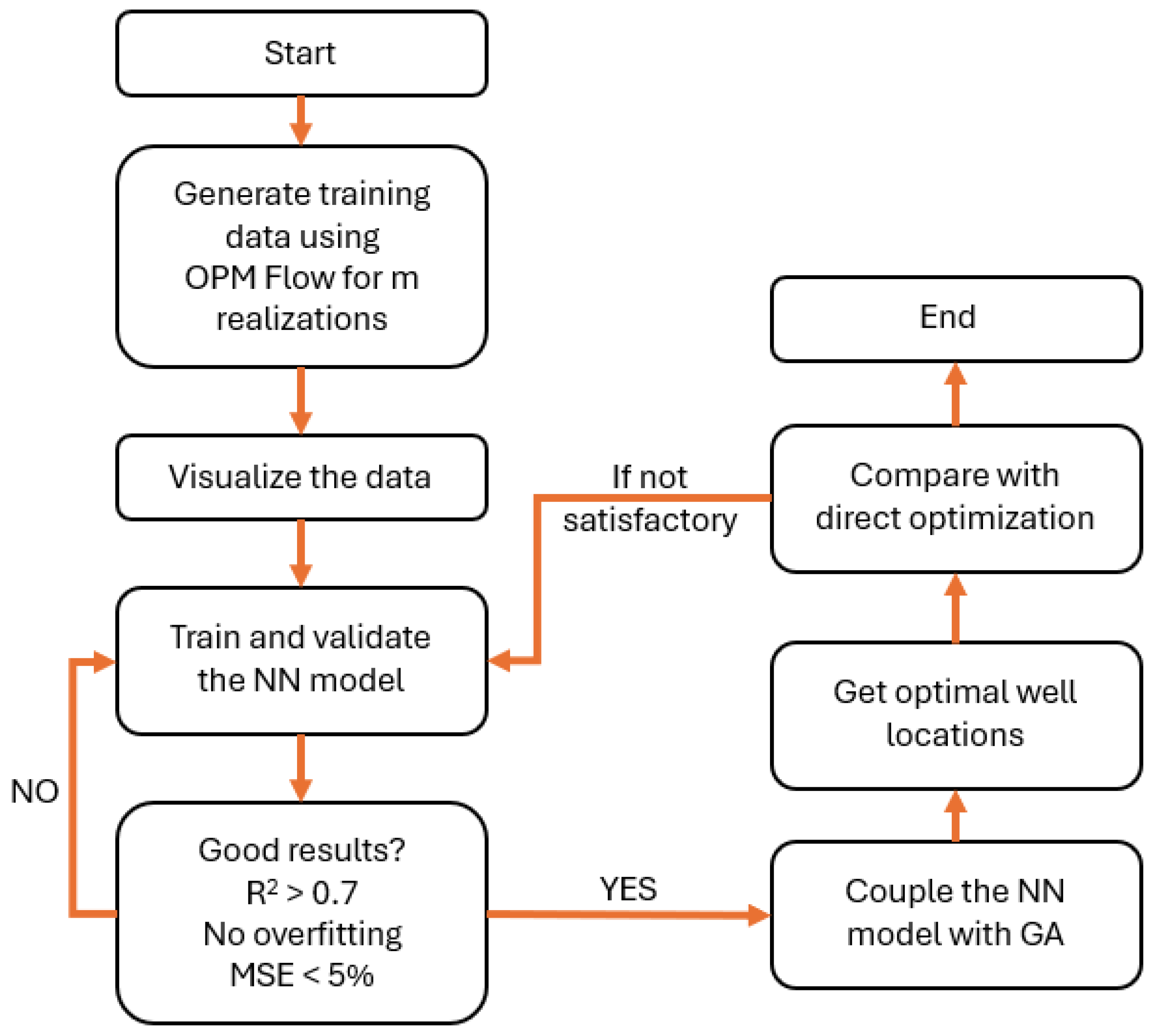
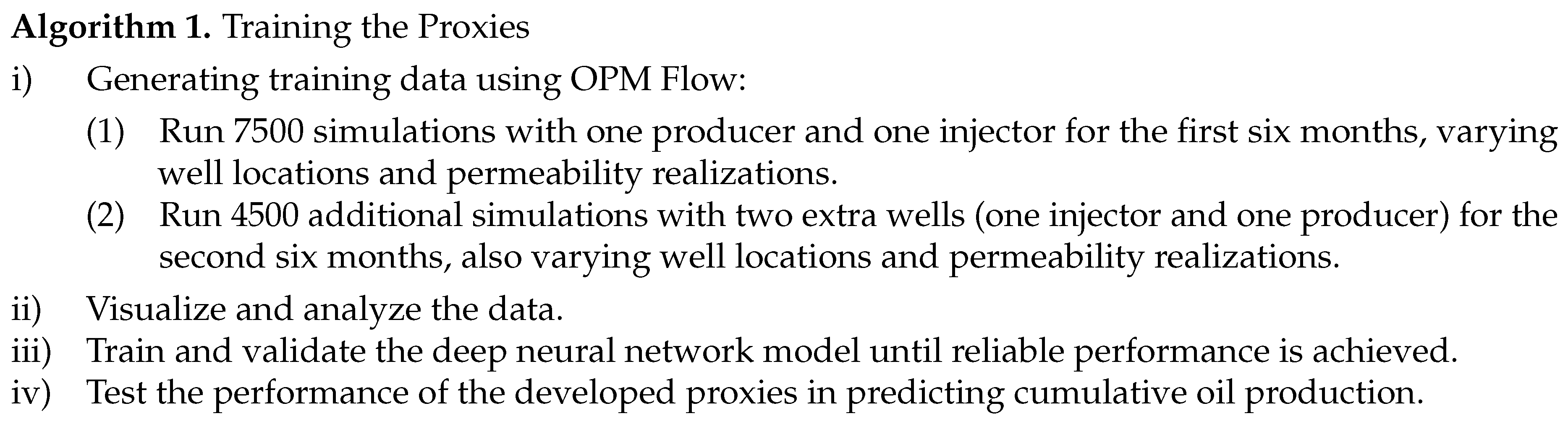
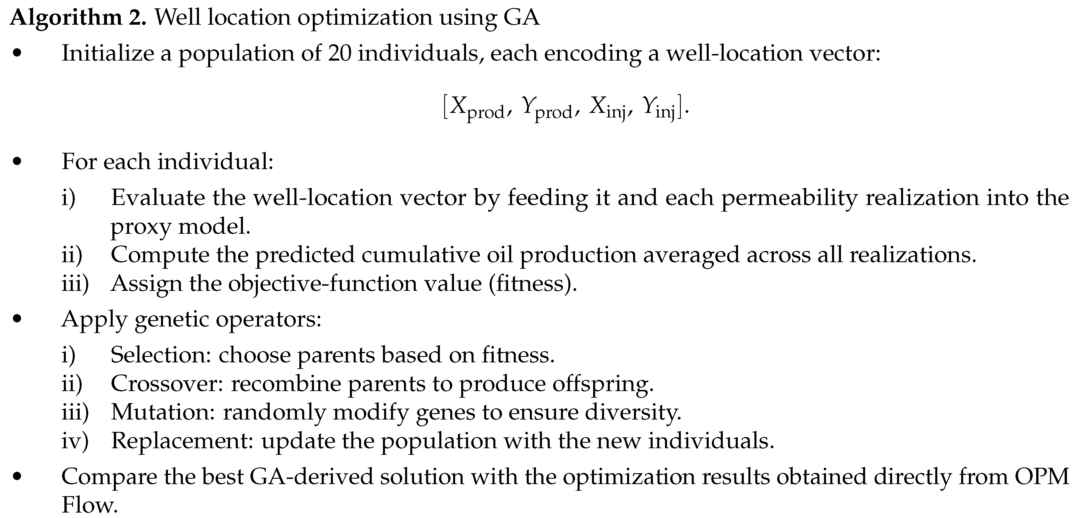
Figure 7.
Flowchart of the methodology for well location optimization.
2.7. Field Description
The Egg Model, first proposed by [38] and later formalized by [39], is a widely adopted synthetic benchmark for evaluating reservoir simulation and optimization methodologies. The model contains 25200 gridblocks, of which 18533 are active, forming an egg-shaped reservoir due to the removal of inactive blocks. Each active cell has a dimension of meters. The standard configuration of the permeability model is illustrated in Figure 8. The geological setting is characterized by meandering high-permeability channels embedded within a background of low-permeability rock, representing the complexity of fluvial depositional systems distributed across seven vertical layers. Because of the strong vertical continuity between the layers, the permeability distribution can be treated as quasi-two-dimensional. This benchmark model is extensively used and well documented in the literature.
A key aspect of the Egg Model is the absence of an underlying aquifer or gas cap, resulting in negligible primary recovery and making waterflooding the dominant drive mechanism. The benchmark is provided as a suite of 101 three-dimensional permeability realizations, each constructed from manually drawn channelized patterns. This stochastic ensemble enables robust evaluation of algorithms under geological uncertainty, supporting studies on reservoir simulation, production optimization, history matching, and closed-loop reservoir management. The full dataset is publicly available and serves as a reference point for comparative research. The geological, fluid, and operational parameters used in this study are summarized in Table 1. The Corey model is employed to compute relative permeabilities, with the specific exponents and endpoint values listed in the table.
In this study, it is assumed that the vertical oil production well if fully penetrating. Accordingly, since there are 3600 gridblocks in the first layer, of which 2491 are active cells, this assumption yields 2491 feasible well placement scenarios, corresponding to the number of active gridblocks in the top layer of the reservoir model.
2.8. Evaluation Metrics
Two evaluation metrics are employed to assess the performance of the proxy models and the proposed optimization framework. The first metric is the coefficient of determination (), which measures how well the variance in the dependent variable can be explained by the independent variable [40]. In this study, the dependent and independent variables correspond to the predicted and actual COP values, respectively. Mathematical expression of the coefficient of determination is given in Equation (14):
where denotes the predicted COP for realization i, and represents the average COP over all realizations. As approaches 1, the predictive capability of the model improves, indicating that a larger portion of the variance in the actual data is captured by the model. From a mathematical standpoint, an value of 1 implies that the variance of the predictions matches the variance of the true values.
The second metric considered is the Mean Absolute Percentage Error (MAPE), which quantifies the relative deviation between predicted and actual COP values. This metric highlights the percentage error associated with each prediction. Formulation of MAPE is presented in Equation (15):
3. Results and Discussion
3.1. Data Analysis
The algorithm was implemented considering a one-year field development plan. The plan assumes the drilling of two wells (one injector and one producer) after each 6-month period, starting from an undeveloped field. For each period, a dataset was generated using OPM Flow reservoir simulation based on the standard Egg model. The dataset consisted of random well locations and random permeability realizations as inputs, while the cumulative oil production served as the output variable.
The dataset sizes for the first and second periods were 7500 and 4500 samples, respectively. Each dataset was divided into 70% training, 20% validation, and 10% testing, ensuring that all subsets preserved comparable statistical characteristics. This distribution was essential to improve the robustness and generalization capability of the neural network model. The statistical distribution of the data for each period is presented in Figure 9 and Figure 10.
3.2. Neural Network Model
Once the dataset was imported, split, and normalized, the next step consisted of defining the initial neural network architecture. The model was designed with two separate input branches: (i) Input branch 1, which receives the permeability realizations represented as 3D arrays and processes them through a sequence of convolutional and pooling layers, and (ii) Input branch 2, which receives the normalized well-location coordinates as a 1D vector and processes them using fully connected layers. The final output of the network is the cumulative oil production expressed in standard cubic meters (sm3).
The proposed architecture is therefore a multi-input neural network, as it integrates two distinct sources of information. In the convolutional branch, the 3D permeability images are passed through several convolutional filters and pooling operations to extract spatial patterns, which are subsequently flattened into a 1D vector. In parallel, the dense branch transforms the normalized well-location inputs through a series of hidden layers. After these transformations, the outputs of both branches—each expressed as a 1D representation—are concatenated into a single feature vector. This combined vector is then processed by an additional set of fully connected layers until the final regression output is obtained. The overall multi-input architecture described above is illustrated in Figure 11, which summarizes the flow of information from each input branch to the final output layer.
Since the performance of the neural network is strongly dependent on its hyperparameters, a systematic tuning process was conducted. A random search strategy was adopted to explore a wide range of configurations, and the best combination of hyperparameters was selected based on the minimization of the validation loss. The hyperparameters investigated included the optimizer, kernel sizes, activation functions, number of convolutional layers, number of filters, pooling sizes, dropout rates, number of dense layers, and learning rate. Table 2 summarizes the optimal hyperparameter values as well as the corresponding ranges explored during the random search.
Figure 12 shows the convergence curves of the proxy model developed for the Egg model, presenting the evolution of the training and validation losses with respect to the number of epochs for both the first and second periods. As observed, the curves do not exhibit a significant gap between the training and validation losses, which may indicates the absence of overfitting. In addition, Figure 13 illustrates the ability of the neural network to predict the cumulative oil production for the training and testing subsets in each period.
For the first period, where the dataset contained 7500 samples, the model performance was regarded as satisfactory. The mean absolute percentage error (MAPE) was approximately 2.0% for the testing subset and about 2.1% for the validation subset. The coefficients of determination corroborate this result, with for the training subset and for the testing subset, indicating that the network was able to learn representative patterns while maintaining reasonable generalization.
For the second period, which included the additional wells and employed a dataset of 4500 samples, the model performance exhibited a slightly higher value for the training subset, despite the reduced amount of data, indicating that the network was still able to extract meaningful patterns from the smaller dataset. The convergence behavior shown in Figure 12 reveals that the validation loss fluctuates more noticeably across epochs. Early stopping was therefore applied, halting training whenever the validation loss failed to improve for 10 consecutive epochs. Even with these fluctuations, the final performance remained consistent with the expected learning capacity given the smaller dataset.
In this second period, the coefficients of determination were for the training subset and for the testing subset. Although the higher training score might appear to indicate overfitting, measures explained variance and may hide generalization deficiencies, so it should not be used alone for this diagnosis. This concern is mitigated by the close agreement between training and validation losses across epochs. The small difference between these curves supports the interpretation that the model remained reliable, even though the values were lower than those obtained in the first period for the testing subset.
Overall, the results indicate that the neural network produces accurate approximations of cumulative oil production for both periods, with its predictive quality naturally influenced by the size of the available training dataset.
3.3. Results of the Period I
The optimization run with the proxy model and the GA yielded a cumulative oil production of 14524 sm3 and is considered the optimal well-location scenario for the first period. Thus, the coordinates presented in Table 3 correspond to the optimal placement of the first two wells.
Figure 14 (left) shows the optimal location of the wells on the permeability distribution map for the first period. As discussed earlier, placing wells along high-permeability channels enhances production, and the proxy reproduced the spatial trend expected from high-permeability channels for the Egg model. This capability is attributed to the convolutional branch of the model, which analyzes the permeability images and identifies spatial structures associated with improved flow performance. In this optimal configuration, the producer is positioned near the central high-permeability channel, whereas the injector is located in a region of lower permeability at the bottom-left of the reservoir model.
Since the main purpose of employing proxy models is to accelerate the optimization process, a comparison of computational costs between the direct optimization and the proxy-based optimization is presented in Table 4. From this comparison, it is observed that the neural network proxy model identified the optimal well locations for the first period using only 26.3% of the computational time required by the direct simulation-based optimization. Additionally, the proxy-based optimization provided results of 4% error in terms of cumulative oil production when compared to the direct simulation output.
This demonstrates that integrating neural network proxies into reservoir optimization workflows is a viable and efficient solution. The percentage of computational time saved by employing the proxy-based optimization is computed as follows:
3.4. Results of the Period II
After determining the optimal well locations for the first period, these wells were fixed at their respective optimal positions and two additional wells were introduced into the reservoir model. The locations of these two new wells were optimized using both the direct optimization strategy and the proxy-based optimization with the GA. As performed previously, the direct optimization was repeated three times to account for the stochastic nature of the GA procedure. The optimization results obtained from the proxy-based approach for the second period are summarized in Table 5. Furthermore, the optimal locations of the two new wells, together with the optimal wells from the first period, are illustrated in Figure 14 (right).
As shown in Fig. 14 (right), the well configuration obtained for the second period presents a consistent spatial pattern relative to the permeability distribution. The new producer (PROD2) is positioned on the right side of the reservoir, directly over a high-permeability channel, which favors higher productivity. The second injector (INJECT2), in turn, is located near PROD1 and also lies on a high-permeability trend, which helps sustain pressure in the main flow pathway feeding both producers. The first injector (INJECT1), positioned at the upper-left corner of the reservoir, remains in a low-permeability region and plays a complementary pressure-maintenance role by supporting the flow toward the central high-permeability channels. This overall placement reflects a consistent configuration in which producers are aligned with high-permeability channels to maximize flow capacity, while injectors maintain reservoir pressure and support sweep efficiency across the reservoir volume.
Since the dataset size for the second period (4500 samples) was smaller than that available for the first period, the computational cost of training the proxy model was reduced significantly. The comparison of computational effort between the proxy-based and direct optimization approaches for this period is presented in Table 6.
The percentage of time saved by utilizing the proxy-based optimization in the second period is calculated as:
From these results, it is evident that the proxy model required only a small fraction of the computational time demanded by the direct simulator. For the first period, the proxy-based optimization required approximately 26% of the time of a full simulation-based optimization, whereas in the second period, it required only about 15%. In practical terms, this represents more than a fivefold reduction in computational effort when replacing direct optimization with proxy-based optimization in the second period.
Despite the substantial time savings, the proxy-based optimization maintained reliable predictive accuracy. For both periods, the proxy model identified well-placement scenarios that produced cumulative oil volumes within a 5% error margin relative to those obtained through direct simulation. These results reinforce that the deep learning–based proxy is an effective and computationally efficient tool for optimizing well locations under geological uncertainty.
4. Conclusions
This work presented a multi-input proxy model composed of convolutional and fully connected layers to approximate, with high fidelity, the reservoir simulator in a two-stage well-placement optimization workflow under geological uncertainty. The proposed proxy receives permeability realizations together with well-location coordinates and predicts the COP for each stage of the development plan, in which a producer and an injector are added at each period.
Using the Egg reservoir model, the proxy demonstrated strong predictive capability, achieving coefficients of determination of 0.76 and 0.82 for the training data in the first and second periods, respectively. In addition to its predictive accuracy, the methodology substantially reduced computational cost. The proxy-based optimization required only about 26% of the time needed for direct simulation in the first period and approximately 15% in the second period, while preserving the optimal COP values within an error margin below 4% and 5%, respectively.
An important contribution of the study is the two-stage strategy, in which separate proxy models are trained for each development stage, mimicking realistic scenarios where wells are drilled sequentially over time. The findings indicate that the proposed framework is a reliable and efficient alternative for determining optimal well placements under geological uncertainty, significantly accelerating the optimization process without relying solely on full-physics reservoir simulations.
Author Contributions
Conceptualization, W.N. and K.F.; methodology, W.N. and K.F.; software, W.N.; validation, W.N. and K.F.; formal analysis, K.F.; investigation, W.N.; resources, W.N. and K.F.; data curation, W.N.; writing—original draft preparation, W.N.; writing—review and editing, K.F.; visualization, W.N.; supervision, K.F., M.P. and M.D.; project administration, K.F.; funding acquisition, M.P. All authors have read and agreed to the published version of the manuscript.
Funding
This research received no external funding.
Institutional Review Board Statement
Not applicable.
Informed Consent Statement
Not applicable.
Data Availability Statement
The data presented in this study are available on request from the corresponding author.
Acknowledgments
This study was financed in part by the Coordenação de Aperfeiçoamento de Pessoal de Nível Superior - Brasil (CAPES). The corresponding author acknowledges the financial support provided by Petrobras.
Conflicts of Interest
The authors declare no conflicts of interest.
References
- Forouzanfar, F.; Li, G.; Reynolds, A. C. A two-stage well placement optimization method based on adjoint gradient. SPE Annual Technical Conference and Exhibition, SPE-135304-MS. Florence, Italy, 19-22 September, 2010. [Google Scholar]
- Bangerth, W.; Klie, H.; Wheeler, M. F.; Stoffa, P. L.; Sen, M. K. On optimization algorithms for the reservoir oil well placement problem. Comput. Geosci. 2006, 10, 303–319. [Google Scholar] [CrossRef]
- Sarma, P.; Chen, W. H. Efficient well placement optimization with gradient-based algorithms and adjoint models. Intelligent Energy Conference and Exhibition, SPE-112257-MS. Amsterdam, The Netherlands, 25-27 February, 2008. [Google Scholar]
- Bittencourt, A. C.; Horne, R. N. Reservoir development and design optimization. SPE Annual Technical Conference and Exhibition, SPE-38895-MS. San Antonio, Texas, USA, 5-8 October, 1997. [Google Scholar]
- Lee, J. W.; Park, C.; Kang, J. M.; Jeong, C. K. Horizontal well design incorporated with interwell interference, drilling location, and trajectory for the recovery optimization. SPE/EAGE Reservoir Characterization and Simulation Conference, SPE-125539-MS. Abu Dhabi, UAE, 19-21 October, 2009. [Google Scholar]
- Rahim, S.; Li, Z. Well placement optimization with geological uncertainty reduction. IFAC-PapersOnLine 2015, 48, 57–62. [Google Scholar] [CrossRef]
- Babaei, M.; Alkhatib, A.; Pan, I. Robust optimization of subsurface flow using polynomial chaos and response surface surrogates. Comput. Geosci. 2015, 19, 979–998. [Google Scholar] [CrossRef]
- Al-Dogail, A. S.; Baarimah, S. O.; Basfar, S. A. Prediction of inflow performance relationship of a gas field using artificial intelligence techniques. SPE Kingdom of Saudi Arabia Annual Technical Symposium and Exhibition, SPE-192273-MS. Dammam, Saudi Arabia, 23-26 April, 2018. [Google Scholar]
- Adeyemi, B. J.; Sulaimon, A. A. Predicting wax formation using artificial neural network. Nigeria Annual International Conference and Exhibition, SPE-163026-MS. Lagos, Nigeria, 6-8 August, 2012. [Google Scholar]
- An, P.; Moon, W. Reservoir characterization using feedforward neural networks. SEG Annual Meeting, SEG-1993-0258. Washington, DC, USA, 26-30 September, 1993. [Google Scholar]
- Long, W.; Chai, D.; Aminzadeh, F. Pseudo density log generation using artificial neural network. SPE Western Regional Meeting, SPE-180439-MS. Anchorage, Alaska, USA, 23-26 May, 2016. [Google Scholar]
- Costa, L. A. N.; Maschio, C.; Schiozer, D. J. Application of artificial neural networks in a history matching process. J. Petrol. Sci. Eng. 2014, 123, 30–45. [Google Scholar] [CrossRef]
- Kim, S.; Min, B.; Kwon, S.; Chu, M.-G. History matching of a channelized reservoir using a serial denoising autoencoder integrated with ES-MDA. Geofluids 2019, 1–22. [Google Scholar] [CrossRef]
- Hamam, H.; Ertekin, T. A generalized varying oil compositions and relative permeability screening tool for continuos carbon dioxide injection in naturally fractured reservoirs. SPE Kingdom of Saudi Arabia Annual Technical Symposium and Exhibition, SPE-192194-MS. Dammam, Saudi Arabia, 23-26 April, 2018. [Google Scholar]
- Jeong, H.; Sun, A.; Jeon, J.; Min, B.; Jeong, D. Efficient ensemble-based stochastic gradient mehotds for optimization under geological uncertainty. Front. Earth Sci. 2020, 8, 1–14. [Google Scholar] [CrossRef]
- Khan, M. R.; Tariq, Z.; Abdulraheem, A. Utilizing state of the art computational intelligence to estimate oil flow rate in artificial lift wells. SPE Kingdom of Saudi Arabia Annual Technical Symposium and Exhibition, SPE-192321-MS. Dammam, Saudi Arabia, 23-26 April, 2018. [Google Scholar]
- El-Sawy, A.; EL-Bakry, H.; Loey, M. CNN for handwritten Arabic digits recognition based on LeNet-5. 2nd International Conference on Advanced Intelligent Systems and Informatics, Cairo, Egypt, 24-26 October, 2016. [Google Scholar]
- Behnke, S. Hierarchical Neural Networks for Image Interpretation; Springer: New York, USA, 2003. [Google Scholar]
- Zhong, Z.; Carr, T. R.; Wu, X.; Wang, G. Application of convolutional neural network in permeability prediction: a case study in the Jacksonburg-Stringtown oil field, West Virginia, USA. Geophysics 2019, 84, B363–B373. [Google Scholar] [CrossRef]
- Chu, M. G.; Min, B.; Kwon, S.; Park, G.; Kim, S.; Huy, N. X. Determination of an infill well placement using a data-driven multi-modal convolutional neural network. J. Petrol. Sci. Eng. 2020, 195, 106805. [Google Scholar] [CrossRef]
- Kim, J.; Yang, H.; Choe, J. Robust optimization of the locations and types of multiple wells using CNN based proxy models. J. Petrol. Sci. Eng. 2020, 193, 107424. [Google Scholar] [CrossRef]
- Miyagi, A.; Akimoto, Y.; Yamamoto, H. Well placement optimization under geological statistical uncertainty. The Genetic and Evolutionary Computation Conference, Prague, Czech Republic, 13-17 July, 2019. [Google Scholar]
- Choi, S.; Oh, H. Improved Extrapolation Mehods of Data-Driven Background Estimation in HIgh-Energy Physics. arXiv 2019, arXiv:1906.10831. [Google Scholar]
- Garcia, J.; Peña, M. Robust optimization: concepts and applications. In Nature-inspired Methods for Stochastic, Robust and Dynamic Optimization; Ser, J.D., Osaba, E., Eds.; IntechOpen: London, 2018; pp. 7–22. [Google Scholar]
- Jesmani, M.; Jafarpour, B.; Bellout, M. C.; Foss, B. A reduced random sampling strategy for fast robust well placement optimization. J. Petrol. Sci. Eng. 2020, 184, 106414. [Google Scholar] [CrossRef]
- Holland, J. H. Adaptation in Natural and Artificial Systems: an Introductory Analysis with Applications to Biology, Control, and Artificial Intelligence; MIT Press: USA, 1992. [Google Scholar]
- Emerick, A. A.; Silva, E.; Messer, B.; Almeida, L. F.; Szwarcman, D.; Pacheco, M. A. C.; Vellasco, M. M. B. R. Well Placement Optimization Using a Genetic Algorithm With Nonlinear Constraints. SPE Reservoir Simulation Symposium, SPE-118808-MS. The Woodlands, Texas, USA, 2-4 February, 2009. [Google Scholar]
- Montes, G.; Bartolome, P.; Udias, A. L. The Use of Genetic Algorithms in Well Placement Optimization. SPE Latin American and Caribbean Petroleum Engineering Conference, SPE-69439-MS. Buenos Aires, Argentina, 25-28 March, 2001. [Google Scholar]
- Wang, N.; Chang, H.; Zhang, D.; Xue, L.; Chen, Y. Efficient well placement optimization based on theory-guided convolutional neural network. J. Pet. Sci. Eng. 2022, 208, 109545. [Google Scholar] [CrossRef]
- Russell, S.; Norvig, P. Artificial Intelligence: a Modern Approach; Prentice Hall: New Jersey, USA, 2002. [Google Scholar]
- Mass, A. L.; Hannun, A. Y.; Ng, A. Y. Rectifier nonlinearities improve neural network acoustic models. 30th International Conference on Machine Learning, JMLR: W&CP 28. Atlanta, Georgia, USA, 16-21 June, 2013. [Google Scholar]
- Glorot, X.; Bordes, A.; Bengio, Y. Deep Sparse Rectifier Neural Networks. 14th International Conference on Artificial Intelligence and Statistics, JMLR: W&CP 15. Fort Lauderdale, Florida, USA, 11-13 April, 2011. [Google Scholar]
- Rumelhart, D. E.; Hinton, G. E.; Williams, R. J. Learning Internal Representations by Error Propagation; ICS-8506; California Univ. San Diego La Jolla Inst. For Cognitive Science, 1985. [Google Scholar]
- LeCun, Y.; Boser, B.; Denker, J. S.; Henderson, D.; Howard, R. E.; Hubbard, W.; Jackel, L. D. Backpropagation Applied to Handwritten Zip Code Recognition. Neural Comput. 1989, 1(4), 541–551. [Google Scholar] [CrossRef]
- Kwon, S.; Park, G.; Jang, Y.; Cho, J.; Chu, M.; Min, B. Determination of oil well placement using convolutional neural network coupled with robust optimization under geological uncertainty. J. Petrol. Sci. Eng. 2021, 201, 108118. [Google Scholar] [CrossRef]
- O’Shea, K.; Nash, R. An Introduction to Convolutional Neural Networks. arXiv 2015, arXiv:1511.08458. [Google Scholar] [CrossRef]
- Rasmussen, A. F.; Sandve, T. H.; Bao, K.; Lauser, A.; Hove, J.; Skaflestad, B.; Klöfkorn, R.; Blatt, M.; Rustad, A. B.; Sævareid, O.; Lie, K.; Thune, A. The Open Porous Media Flow Reservoir Simulator. Comput. Math. Appl. 2021, 81, 159–185. [Google Scholar] [CrossRef]
- Van Essen, G. M; Zandvliet, M. J.; Van den Hof, P. M. J.; Bosgra, O. H.; Jansen, J. D. Robust Waterflooding Optimization of Multiple Geological Scenarios. SPE Journal 2009, 14, 202–210. [Google Scholar] [CrossRef]
- Jansen, J. D.; Fonseca, R. M.; Kahrobaei, S.; Siraj, M. M.; Van Essen, G. M; Van den Hof, P. M. J. The egg model - a geological ensemble for reservoir simulation. Geoscience Data Journal 2014, 1, 192–195. [Google Scholar] [CrossRef]
- Wu, C.; Jin, L.; Zhao, J.; Wan, X.; Jiang, T.; Ling, K. Determination of Gas-Oil minimum miscibility pressure for impure CO2 through optimized machine learning models. Geoenergy Sci. Eng. 2024, 242, 213216. [Google Scholar] [CrossRef]
- Yousefzadeh, R.; Kazemi, A.; Al-Hmouz, R.; Al-Moosawi, I. Determination of optimal oil well placement using deep learning under geological uncertainty. Geoenergy Sci. Eng. 2025, 246, 213621. [Google Scholar] [CrossRef]
Figure 1.
Flowchart of the genetic algorithm. Adapted from [29].
Figure 1.
Flowchart of the genetic algorithm. Adapted from [29].
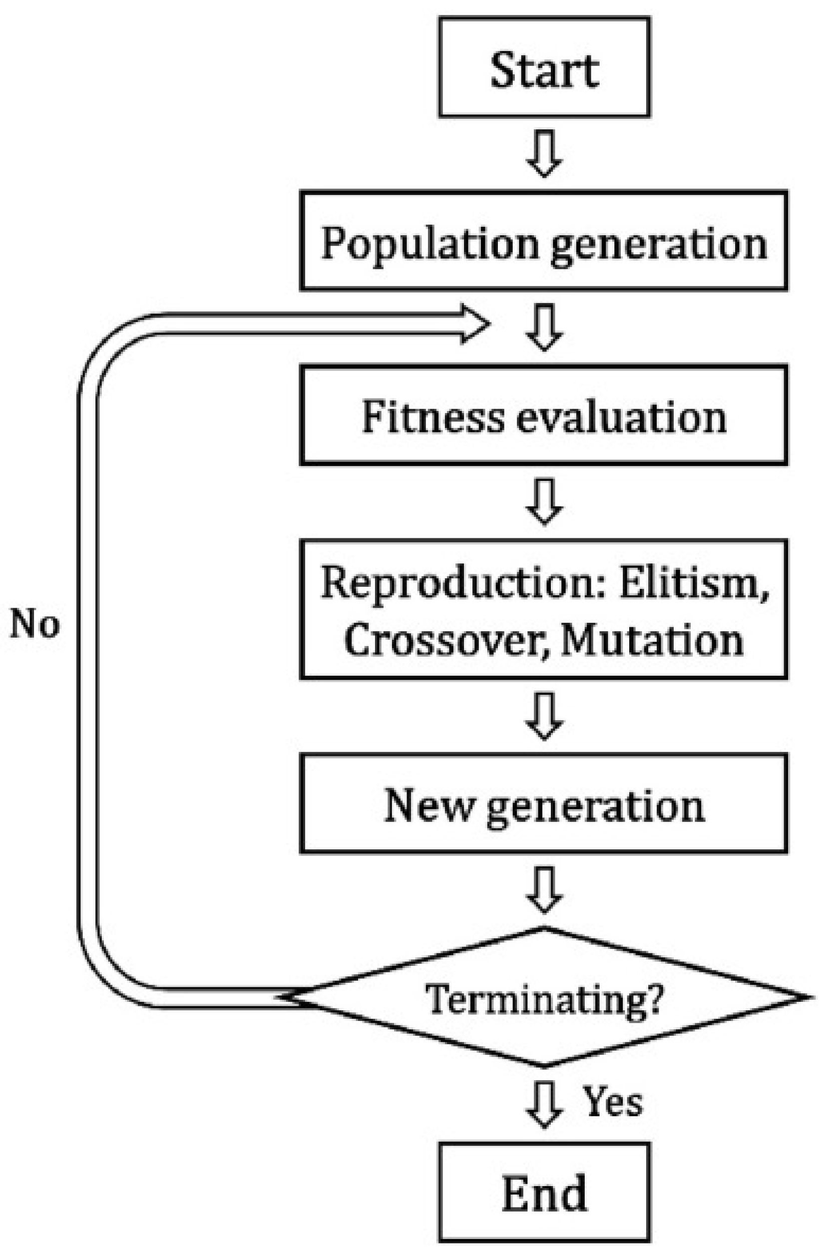
Figure 2.
Schematic of a fully connected ANN. Adapted from [20].
Figure 2.
Schematic of a fully connected ANN. Adapted from [20].
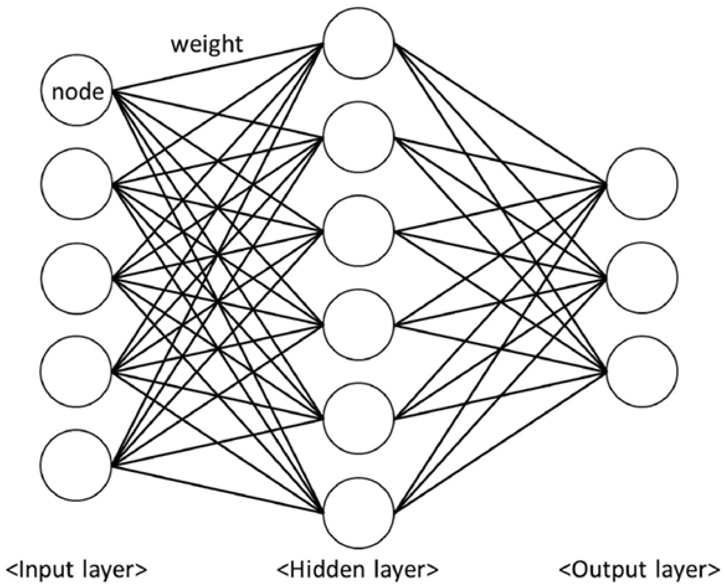
Figure 3.
Activation functions for NN: (a) Sigmoid, (b) Hyperbolic tangent, (c) Linear, (d) ReLU. Adapted from [20].
Figure 3.
Activation functions for NN: (a) Sigmoid, (b) Hyperbolic tangent, (c) Linear, (d) ReLU. Adapted from [20].
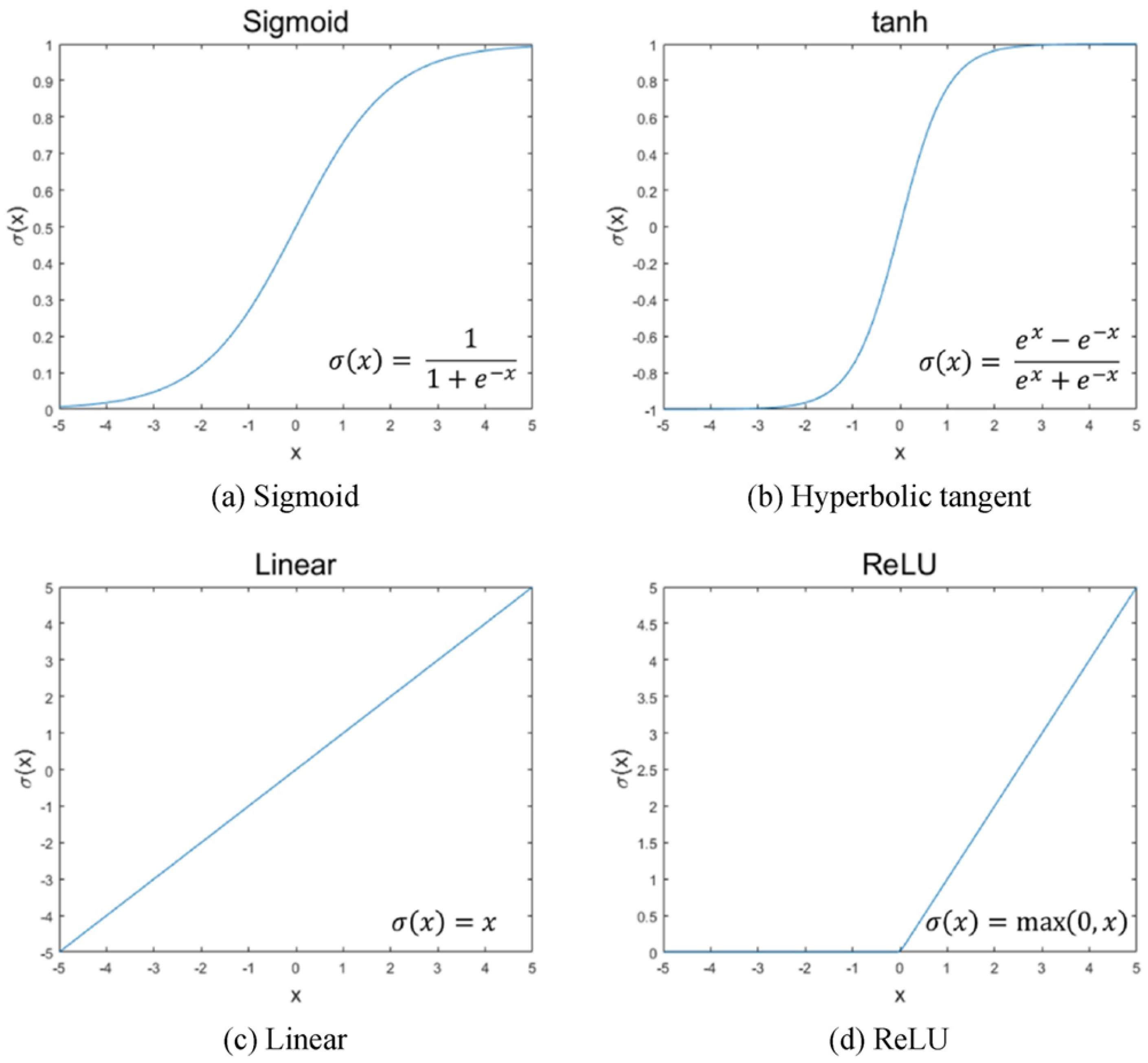
Figure 4.
Schematic of a CNN. Adapted from [35].
Figure 4.
Schematic of a CNN. Adapted from [35].
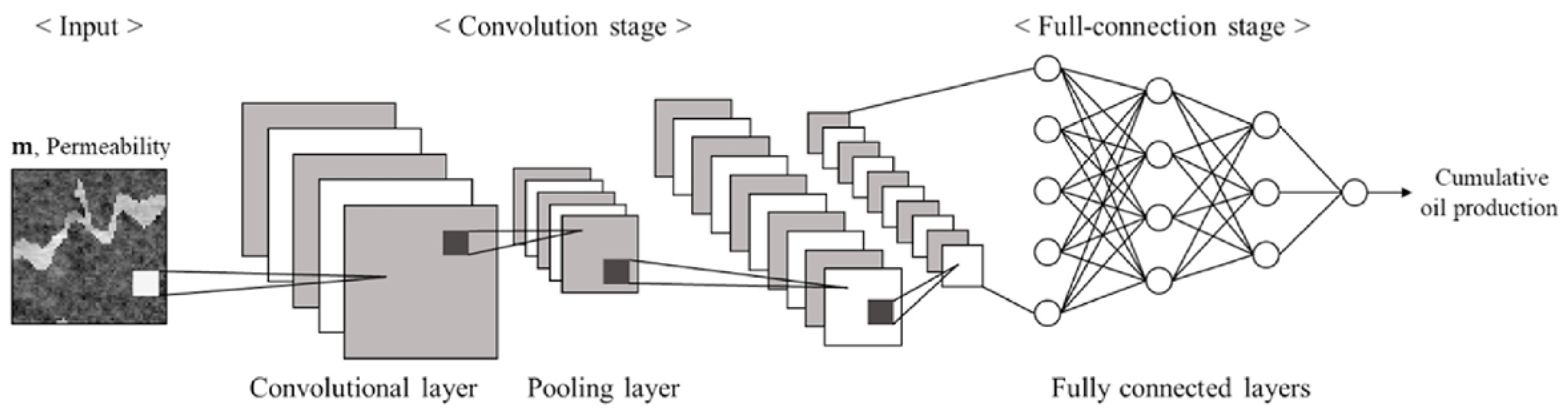
Figure 5.
Schematic of convolution for a 2D data array. Adapted from [20].
Figure 5.
Schematic of convolution for a 2D data array. Adapted from [20].
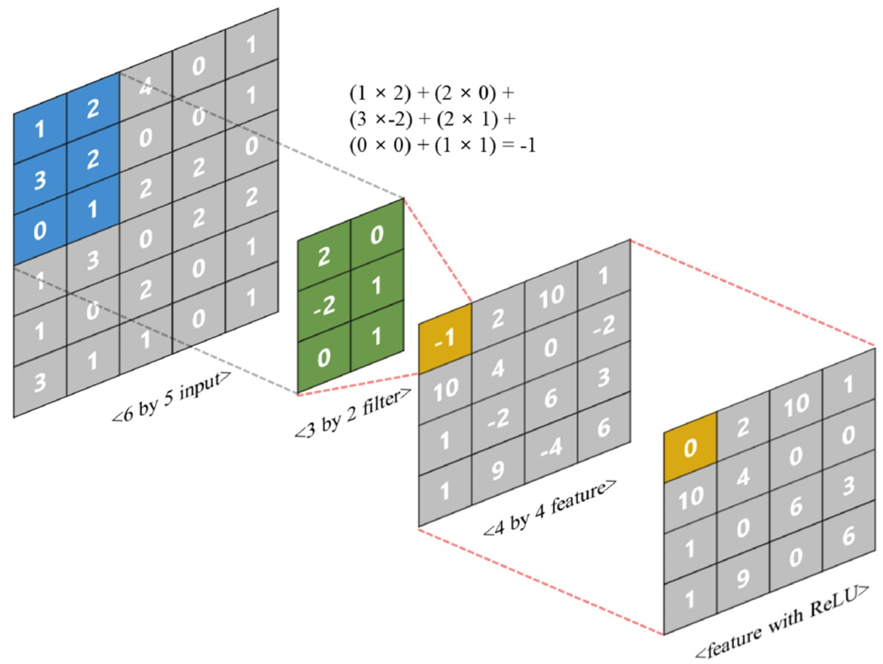
Figure 6.
Schematic of max pooling for a 2D data array. Adapted from [20].
Figure 6.
Schematic of max pooling for a 2D data array. Adapted from [20].
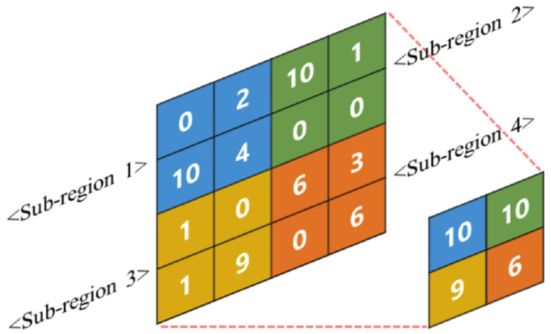
Figure 8.
3D Egg model: permeability distribuition of the deterministic version.
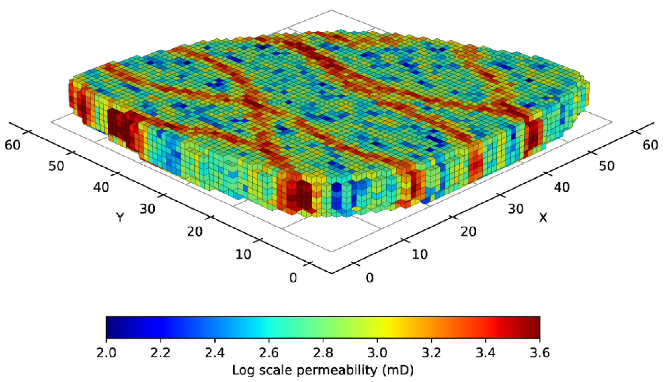
Figure 9.
Data visualization for the first period.
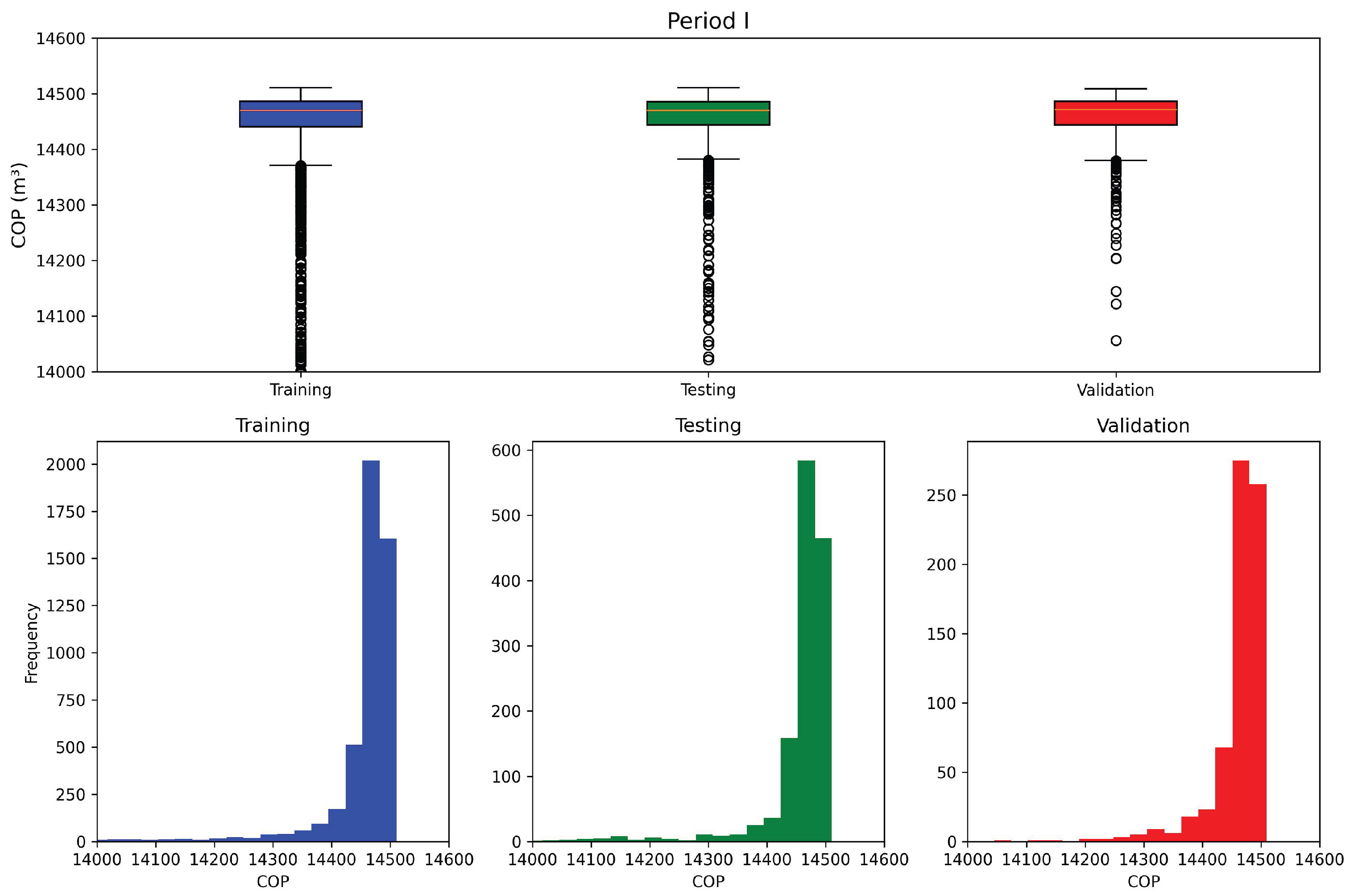
Figure 10.
Data visualization for the second period.
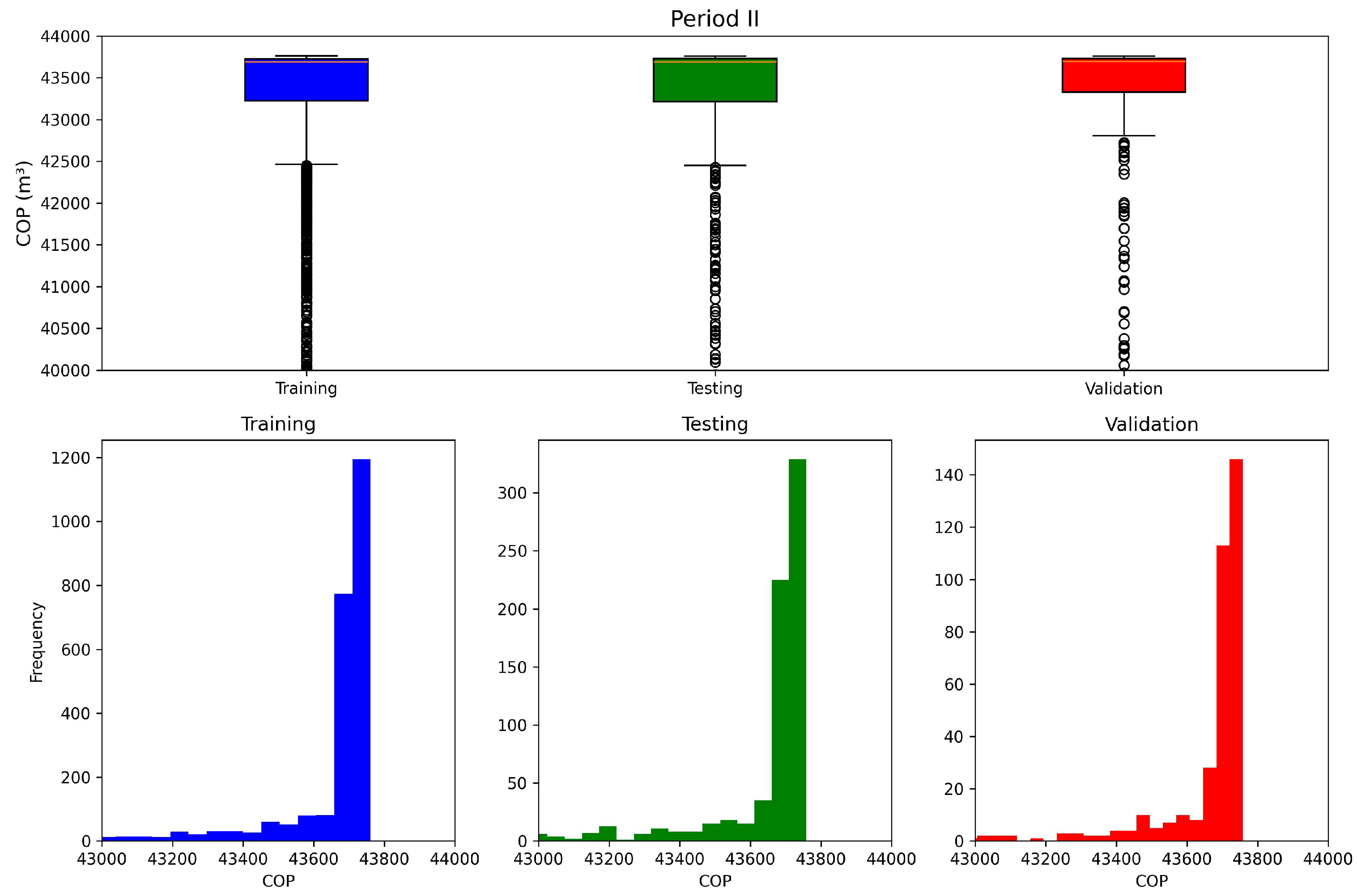
Figure 11.
Schematic of the proposed architecture for the proxy models. Adapted from [41].
Figure 11.
Schematic of the proposed architecture for the proxy models. Adapted from [41].
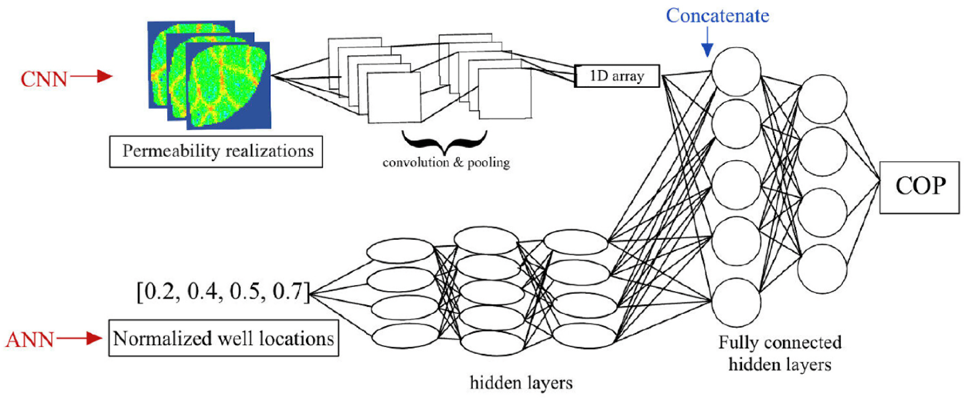
Figure 12.
Loss versus Epoch for Period I (left) and Period II (right).
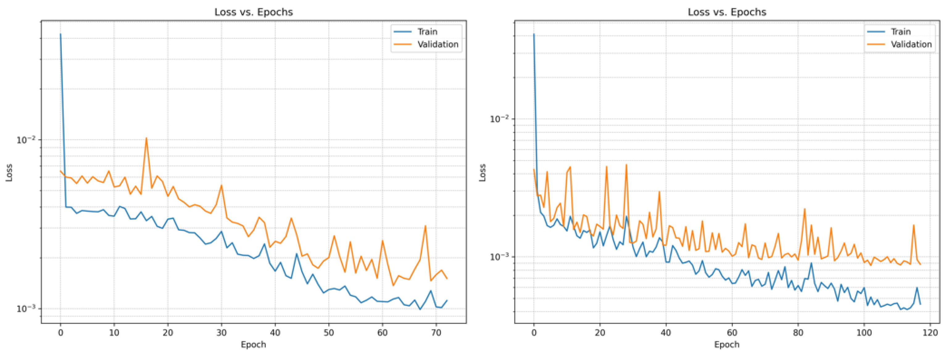
Figure 13.
Cross-plots of predict and actual COPs for Period I (left) and Period II (right).
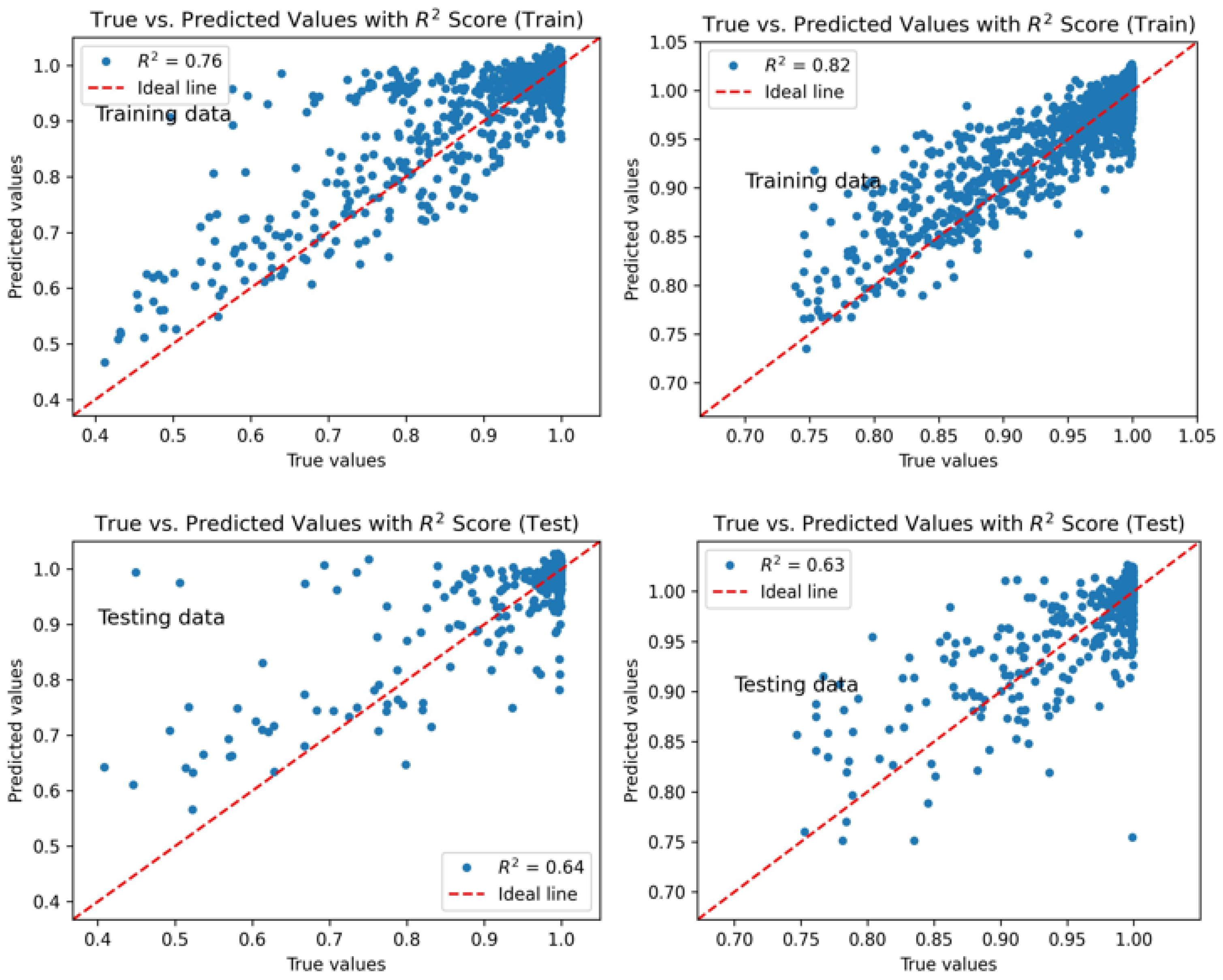
Figure 14.
Optimal well locations for Period I (left) and Period II (right).
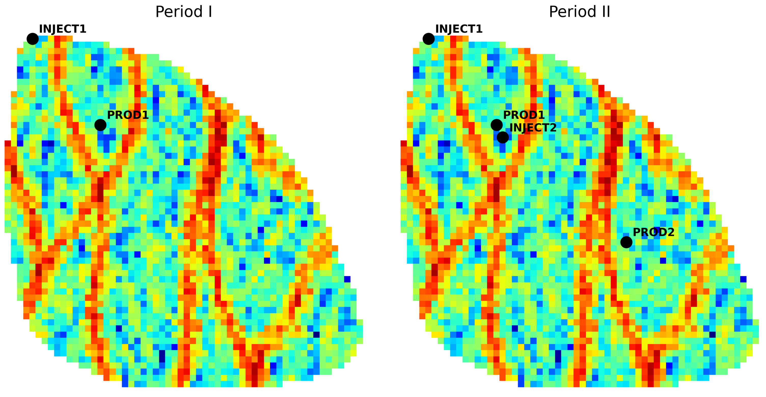

Table 1.
Reservoir and fluid properties for the Egg Model.
| Property | Value | Unit |
|---|---|---|
| Dimensions | – | |
| Cell dimension size | m | |
| Water injection rate | 79.5 | m3/day |
| Well pressure | Pa | |
| Corey exponent for oil | 4 | – |
| Corey exponent for water | 3 | – |
| Connate water saturation | 20 | % |
| Initial water saturation | 10 | % |
| Residual oil saturation | 10 | % |
| Relative perm. to oil | 0.8 | – |
| Relative perm. to water | 0.75 | – |
| Capillary pressure | 0 | Pa |
| Porosity | 0.2 | – |
| Reservoir pressure | Pa | |
| Oil compressibility | Pa−1 | |
| Water compressibility | Pa−1 | |
| Rock compressibility | 0 | Pa−1 |
| Oil viscosity | Pa·s | |
| Water viscosity | Pa·s |
Source: Adapted from [39]
Table 2.
Optimal hyperparameters of the proxy models and their investigated ranges/values.
| Hyperparameter | Optimal value | Investigated ranges/values |
|---|---|---|
| Convolutional branch | ||
| # convolutional layers | 2 | 1–4 |
| # kernels | 64, 64 | 16–128 |
| Kernel sizes | 3, 3 | 2, 3, 4, 5 |
| Activation functions | ReLU | ReLU, tanh, sigmoid |
| Pooling size | 3 | 2, 3, 4 |
| Dropout rate | 0.4 | 0.1–0.5 |
| Fully connected / dense branch | ||
| # dense layers | 4 | 1–4 |
| # dense neurons | 432, 32, 336, 112 | 16–512 |
| Dropout rate | 0.5 | 0.1–0.5 |
| Fully connected head (concatenation) | ||
| # dense layers | 3 | 1–8 |
| # dense neurons | 16, 96, 336 | 16–512 |
| Dropout rate | 0.3 | 0.1–0.5 |
| Training settings | ||
| Optimizer | Adam | Adam, SGD, RMSProp |
| Learning rate | 0.0005 | 1E-5 – 1E-2 |
| Loss | Mean Squared Error | – |
| Maximum epochs | 300 | – |
| Batch size | 64 | – |
| Early stopping | True | – |
Table 3.
Optimal results from optimization for period I.
| Parameter | Value |
|---|---|
| Producer Coordinates | (16, 43) |
| Injector Coordinates | (5, 57) |
| Optimal COP from proxy | 14524 sm3 |
| Optimal COP from reservoir simulator | 15000 sm3 |
| MAPE between the true and predicted | 3.2% |
Table 4.
Time comparison between proxy-based and direct optimization approaches in period I.
| Optimization type | Step | # Simulations | Time (mins) |
|---|---|---|---|
| Proxy-based | Data acquisition (OPM Flow) | 7500 | 1250 |
| Proxy training | – | 15 | |
| Optimization | – | 60 | |
| Total = 1325 | |||
| Direct | Optimization | 3×10,000 | 5040 |
Table 5.
Optimal results from optimization for period II.
| Parameter | Value |
|---|---|
| Producer Coordinates | (37, 24) |
| Injector Coordinates | (17, 41) |
| Optimal COP from proxy | 25511 sm3 |
| Optimal COP from reservoir simulator | 26058 sm3 |
| MAPE between the true and predicted | 1.8% |
Table 6.
Time comparison between proxy-based and direct optimization approaches in period II.
| Optimization type | Step | # Simulations | Time (mins) |
|---|---|---|---|
| Proxy-based | Data acquisition (OPM Flow) | 4500 | 820 |
| Proxy training | – | 15 | |
| Optimization | – | 40 | |
| Total = 875 | |||
| Direct | Optimization | 3×10,000 | 5840 |
Disclaimer/Publisher’s Note: The statements, opinions and data contained in all publications are solely those of the individual author(s) and contributor(s) and not of MDPI and/or the editor(s). MDPI and/or the editor(s) disclaim responsibility for any injury to people or property resulting from any ideas, methods, instructions or products referred to in the content. |
© 2026 by the authors. Licensee MDPI, Basel, Switzerland. This article is an open access article distributed under the terms and conditions of the Creative Commons Attribution (CC BY) license (http://creativecommons.org/licenses/by/4.0/).
Copyright: This open access article is published under a Creative Commons CC BY 4.0 license, which permit the free download, distribution, and reuse, provided that the author and preprint are cited in any reuse.


