Submitted:
22 January 2026
Posted:
23 January 2026
You are already at the latest version
Abstract
One of the main obstacles to testing quantum gravity is that genuinely Planckian effects are expected only at energies and curvatures far beyond current experimental reach. I point out that ultrafast, high-intensity lasers, in combination with fourth-generation x-ray light sources, already allow the laboratory production of non-inertial, effectively non-Minkowski space-time regions in which quantum fields experience enormous accelerations over micron-scale distances. By the equivalence principle, these configurations are locally indistinguishable from weak, highly curved gravitational backgrounds. I emphasize a concrete, experimentally motivated observable: the broadening of x-ray Thomson scattering from electrons accelerated in the focus of an extreme laser. This broadening depends on the acceleration and the local effective metric and hence can serve as a controlled probe of quantum mechanics and, ultimately, quantum-gravity-motivated modifications in non-Minkowski space-time.
Keywords:
lasers
; quantum gravity
1. Motivation
A persistent challenge in quantum gravity is the apparent inaccessibility of the Planck scale , which lies orders of magnitude beyond even the most ambitious collider concepts. Naïvely, one might conclude that any direct test of quantum gravity must also be out of experimental reach.
This conclusion is too pessimistic. First, many candidate theories of quantum gravity predict low-energy relics, for example, tiny violations of Lorentz invariance, modified dispersion relations, or nonlocal form factors in effective field theory that can in principle be probed well below the Planck scale. Second, quantum gravity must reduce, in an appropriate limit, to quantum field theory in curved space-time. Demonstrating unambiguously that quantum fields behave as predicted in non-Minkowski backgrounds would therefore already constitute an important semi-classical test on the road to full quantum gravity.
The rise of chirped-pulse amplification (CPA) and petawatt-class systems has made it possible to generate optical pulses with intensities exceeding –, with further orders of magnitude envisioned at facilities such as the Extreme Light Infrastructure and similar high-field centers [1,2]. In such fields, electrons can be accelerated to ultra-relativistic energies within a single optical cycle. These developments motivate the question “can extreme lasers be used as tabletop probes of quantum mechanics — and ultimately quantum gravity — in non-Minkowski space-time?"
The novelty of the present note is twofold. First, we recast the Crowley et al. proposal in the language of Lorentz–invariant nonlocal effective field theories, showing that precision measurements of acceleration–induced broadening in x–ray Thomson scattering can be reinterpreted as laboratory bounds on the nonlocality scale of quantum–gravity inspired propagators, including the entire–function regulator employed in nonlocal QFT [3,4,5,6,7,8,9,10]. Second, we argue that the combination of modern chirped–pulse amplification lasers, fourth–generation x–ray free–electron lasers and ultrahigh–resolution scattering diagnostics renders such experiments technically realistic, and we outline possible quantum–optical extensions based on entangled probes and decoherence [11,12,13,14,15,16]. Together, these developments suggest that intense laser facilities offer a promising, conceptually clean route to probing low–energy imprints of quantum gravity in the laboratory.
2. Acceleration, Equivalence Principle, and Effective Metrics
Lets consider an electron of charge e and rest mass interacting with a strong, classical laser field with electric field amplitude . Ignoring radiation reaction and focusing on the instantaneous dynamics near the focus, a useful estimate of the proper acceleration a experienced by the electron is:
where is the Lorentz factor associated with the electron’s motion. For realistic parameters in current and planned high-intensity facilities, one can reach proper accelerations that are enormous by everyday standards.
Locally, the equivalence principle states that a uniformly accelerated frame in flat space-time is indistinguishable from a frame at rest in a uniform gravitational field. Mathematically, this is encoded in the Rindler metric:
which describes the space-time seen by a uniformly accelerated observer. Quantum fields in this background experience nontrivial phenomena such as Unruh radiation, formally characterized by a thermal spectrum at temperature:
where is Boltzmann’s constant [17,18]. For the extreme accelerations achievable in intense laser fields, the associated Unruh temperature is formally large, although detecting this radiation in practice is highly nontrivial because of short interaction times and competing backgrounds. Related proposals to test Unruh-like effects with ultraintense lasers can be found in Refs. [19,20,21].
The key conceptual point is that extreme laser fields realize, in a small focal region, an effective non-Minkowski geometry for the quantum dynamics of charged particles and photons. This opens an avenue to test how quantum mechanics and potentially its quantum-gravity extensions behaves in a curved or non-inertial space-time.
3. Thomson Scattering in Non-Minkowski Space-time
One particularly clean observable in this context is Thomson scattering of x-ray photons by laser-accelerated electrons. The basic configuration is as follows: an intense optical laser pulse accelerates a population of electrons to ultra-relativistic energies over a short distance near the focal spot. Then a synchronized x-ray pulse from a fourth-generation light source, such as an x-ray free-electron laser is directed through the same interaction region, scattering off the accelerated electrons. The scattered x-ray spectrum is recorded in the laboratory frame with high energy resolution.
In the absence of gravitational or non-inertial effects, the scattering is described by standard relativistic Thomson or Compton scattering in flat Minkowski space-time. Once the electrons are subject to large proper accelerations, their dynamics can be re-expressed in terms of an effective metric that encodes the non-inertial frame. A semiclassical extension of quantum mechanics to this non-Minkowski background predicts that the scattered x-ray line profile acquires an additional broadening that depends on the acceleration and the local metric.
One can write the scattered spectrum as:
where is the standard flat-space Thomson result, is the scattered photon frequency, and encodes the deviation induced by the effective non-Minkowski metric and the electron acceleration a. In more detailed treatments, this deviation can be mapped to a variable-mass metric or a post-Newtonian correction to the Thomson cross section. The crucial point is that the additional broadening is not arbitrary as it scales in a controlled way with a and with the specific structure of the effective metric. By carefully measuring the width and shape of the scattered x-ray line as a function of laser intensity, electron beam parameters, and scattering geometry, one can therefore test the consistency of quantum mechanics in a non-inertial effectively curved space-time, and the presence or absence of additional, quantum-gravity-motivated corrections that might modify the effective metric or the dispersion relations of the particles involved.
4. Experimental Concept with Chirped-Pulse Amplified Lasers
The proposed test of quantum mechanics and, by extension, quantum-gravity-motivated extensions in a non-Minkowski background can be implemented with existing ultrafast, high-intensity laser technology based on chirped pulse amplification [1,2]. Modern Titanium-doped Sapphire (Ti:sapphire) or optical parametric Chirped-pulse Amplification (OPCPA) systems routinely deliver pulses with energies and durations , corresponding to peak powers in the range [1,2]. When focused to a few-micron spot size, these beams reach peak intensities:
providing electric field amplitudes:
at the laser focus. An electron of charge e and mass interacting with such a field experiences a proper acceleration:
where is its Lorentz factor.
Figure 1.
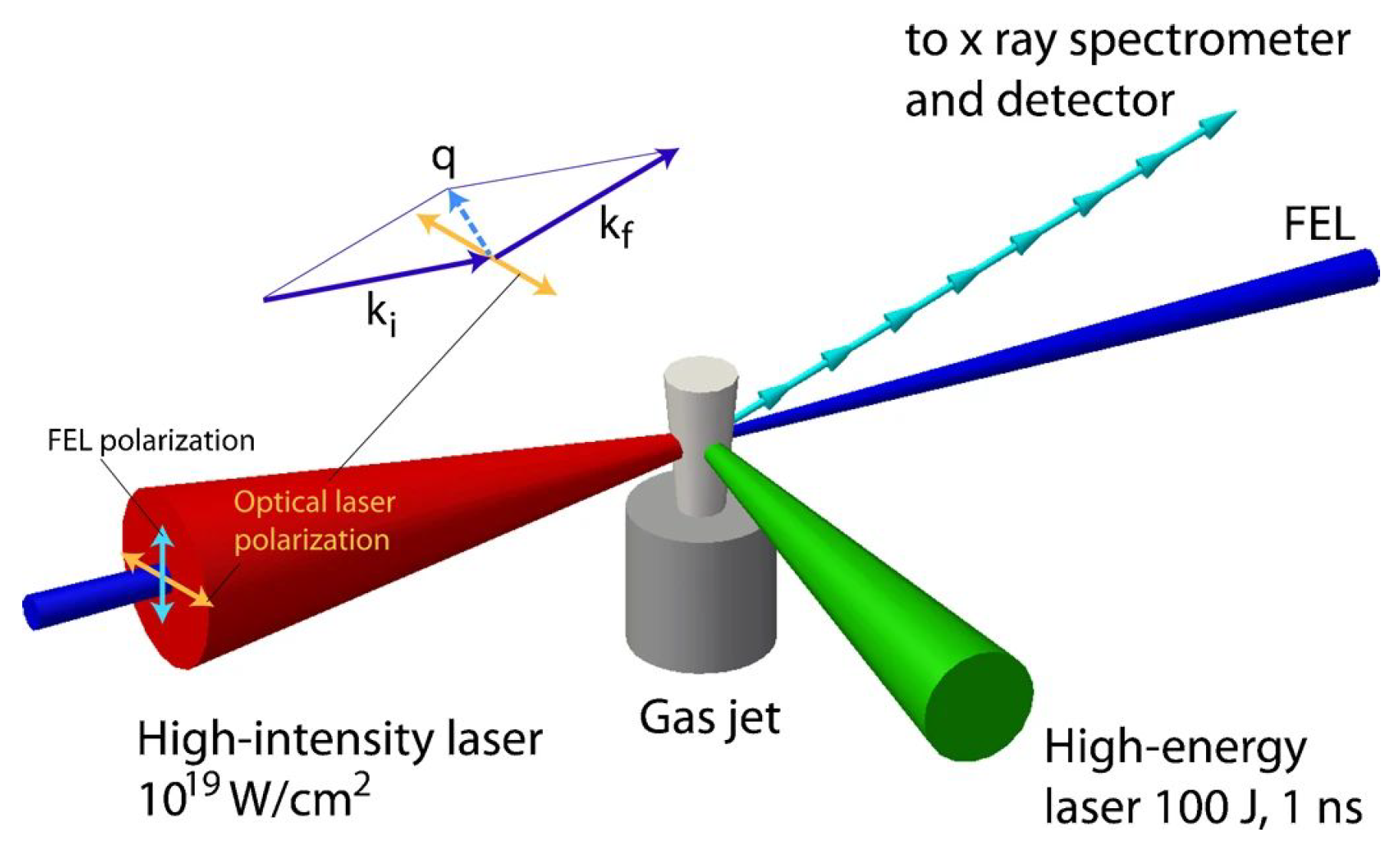
Schematic three-beam configuration. A high-energy ns laser (green) ionizes a low-Z gas jet to form an underdense plasma channel. A high-intensity CPA optical pulse (red) is focused into the channel and accelerates the electrons. An XFEL beam (blue) is overlapped with the interaction region; the scattered x rays are collected by a spectrometer at a fixed angle. The inset shows the incident and scattered x-ray wavevectors , , and the momentum transfer . Adapted from Crowley et al. [22].
Figure 1.
Schematic three-beam configuration. A high-energy ns laser (green) ionizes a low-Z gas jet to form an underdense plasma channel. A high-intensity CPA optical pulse (red) is focused into the channel and accelerates the electrons. An XFEL beam (blue) is overlapped with the interaction region; the scattered x rays are collected by a spectrometer at a fixed angle. The inset shows the incident and scattered x-ray wavevectors , , and the momentum transfer . Adapted from Crowley et al. [22].
For representative parameters and , one finds:
corresponding to an Unruh temperature:
Thus, the CPA focus generates a localized region in which quantum fields evolve under extremely large accelerations, effectively realizing a non-inertial Rindler-like patch of space-time in the laboratory.
Following Crowley et al. [22], we consider a three-beam configuration with a long-pulse (), high-energy laser or discharge pre-ionizes a low-Z gas jet, creating a plasma channel with electron density and temperature . A high-intensity CPA optical beam is focused into this channel and drives a collective acceleration of the electrons, characterized by a controllable proper ponderomotive acceleration . A synchronized x-ray pulse from a fourth-generation light source (XFEL) traverses the same region and undergoes Thomson scattering from the accelerated electrons. Before we move on I will briefly review ponderomotive force and potential as these are important dynamics for the ponderomotive acceleration. Since laser beams are inhomogeneous over their electric fields as it varies spatially, this inhomogeneity is what generates the ponderomotive force. If the field amplitude depends on position:
where or equivalently the laser intensity changes on a length scale L that is large compared with the quiver amplitude and the wavelength. We can split the electron position into a fast quiver piece and a slow drift:
where is the rapid oscillation at and is a slowly varying guiding centre. If we expand the field and the guiding centre:
and solving perturbatively then averaging the equation of motion over one optical cycle gives a secular term in the slow equation of motion of the term:
where:
is the ponderomotive force, and:
is the ponderomotive potential. In the non-relativistic limit is the cycle averaged squared electric field at a point. is the effective energy associated with the quiver motion in the oscillating field.
We know , and , so electrons are pushed out of high intensity regions towards weaker fields. The dependence is proportional to , so the direction of the force does not depend on the sign of the charge, both electrons and positrons are repelled from high intensity regions. In terms of the laser intensity:
the ponderomotive potential can be written as:
, so we can see:
and the ponderomotive acceleration is:
If the intensity changes over a length scale L:
this shows us that a higher intensity gives a stronger ponderomotive acceleration, lower frequencies or longer wavelengths have stronger ponderomotive effects:
and a smaller focuses given by a smaller L has a stronger ponderomotive force.
In the absence of acceleration, the scattered spectrum is described by the usual x-ray Thomson or Compton scattering formalism in Minkowski space-time. In the presence of acceleration, the semiclassical extension of quantum mechanics to a weakly curved or non-inertial metric predicts that the dynamical structure factor acquires an additional, acceleration-dependent contribution. As shown in Ref. [22], the scattered x-ray line can be interpreted as arising from an effective temperature:
where parametrizes the choice of metric and coupling, and grows with the acceleration a. For intensities and soft x-ray probe photons, one finds , which is well within the energy resolution of current x-ray Thomson scattering diagnostics.
The use of CPA lasers is therefore not merely convenient but essential as they provide the ultra-short, ultra-intense fields needed to generate large accelerations over micron-scale distances without damaging the optical components. By scanning the CPA intensity and hence a while monitoring the width and shape of the scattered x-ray line, one can test the predicted dependence , discriminate between different semiclassical curved-space models, and search for small, quantum-gravity-motivated deviations encoded in the effective metric or dispersion relations.
5. Mathematical Framework for Thomson Scattering in an Accelerated Plasma
In this section I summarize, and slightly generalize, the formalism of Crowley et al. for x-ray Thomson scattering from an ensemble of accelerated electrons in a weakly curved or non-inertial space-time. The goal is to make explicit how the measured line shape is controlled by the electron acceleration a, by the choice of effective metric, and by possible quantum-gravity/nonlocal corrections.
We should consider non-relativistic electrons of mass m and charge e confined in a volume V, interacting with an x-ray electromagnetic field in the presence of a weak gravitational or non-inertial background with metric . In the minimal-coupling Hamiltonian, the scattering of x-rays from free electrons is dominated by the term. In the weak field limit one can write the interaction Hamiltonian as can be derived, if we recall that we have a 3-metric with the non-relativistic Hamiltonian of a spinless charged particle with charge e in an extended vector potential :
with .
suppressing the dependence for brevityfrom this we can break it into three Hamiltonians:
where:
in the near flat space limit we know :
For N electrons at a position the total interaction is:
we can explain this in terms of the electron density:
where is the 3-dimensional Dirac delta distribution. We include the so that:
where N is the particle number. From this we find the interaction Hamiltonian:
and we recall that for the weak field :
where is the determinant of the induced spatial metric on the constant-time slice, is the electron density operator at position and time t and is the i-th spatial component of the x-ray vector potential operator at . Summation over repeated spatial indices i is understood. The vector potential can be expanded in normal modes in the usual way:
where is the polarization vector, , and is the photon annihilation operator. Working in the Born approximation, the double differential cross section for scattering an incident photon with frequency and wavevector into a final state with can be written as:
where N is the number of electrons, is the classical electron radius, and are the momentum and frequency transfer, and is the dynamical structure factor, the Van Hove density–density correlator:
with:
the spatial Fourier transform of the electron density operator. Expectation values are taken in the state of the electron gas and x-ray field. In flat space-time and in the absence of acceleration, coincides with the real scattering wavevector and Equation (37) reduces to the standard x-ray Thomson scattering formula.
In principle, electrons couple both to the electromagnetic field through their charge and through their intrinsic magnetic moment, in a nonrelativistic expansion of QED the interaction Hamiltonian for a single electron can be written as:
where and are the vector potential and magnetic field of the x-ray (XFEL) probe, are the Pauli matrices, and is the Bohr magneton. The Thomson scattering channel that enters the dynamic structure factor is generated by the term. The spin-dependent term gives only a small magnetic correction to the x-ray scattering amplitude.
For the parameter range considered here, these magnetic-moment effects are negligible. Numerically, the Bohr magneton has magnitude:
has units of energy per unit magnetic field and matches with the Zeeman term . The associated Zeeman energy scale:
is tiny compared to both the XFEL photon energy () and the electron rest energy (). Thus and .
Moreover, the plasma is unpolarized, and the strong CPA field is treated as a classical driver that defines an effective proper acceleration of the electron ensemble. The Thomson line shape and the effective temperature shift depend only on and on the charge-coupling channel, and are insensitive, at our level of accuracy, to spin-dependent corrections. Magnetic-moment effects therefore contribute only at a negligible level in the scattering cross section and can safely be neglected in the present analysis.
To model the effect of acceleration and gravity on the electrons, Crowley et al. introduce an effective metric in which the electron worldlines are uniformly accelerated along, say, the z axis, while the photon field remains quantized as in Minkowski space. In that formalism the acceleration enters the scattering problem through a complex shift of the scattering wavevector, of the form:
where is a dimensionless parameter characterizing how the metric couples to the electron mass density, for the “variable-mass” metric of Crowley et al., one finds .
A constant drift velocity is an inertial effect as it can be removed by a global Lorentz boost and, in the laboratory frame, it primarily shifts the center frequency of the scattered line Doppler shift. It does not, by itself, generate an intrinsic excess line broadening at fixed geometry and fixed microscopic plasma temperature. The observable proposed here is instead an excess broadening of the Thomson line that persists even when the underlying kinetic temperature T is held fixed. This requires genuinely non-inertial motion. By the equivalence principle, a uniform proper acceleration a defines a local Rindler frame and can be treated as an effective gravitational field for local processes. In the Crowley-type effective-metric description, this non-inertial physics enters the scattering problem through a complex shift of the momentum transfer Equation (43) so that the accelerated structure factor becomes a Gaussian smearing of the equilibrium structure factor in frequency space. Equivalently, the line retains its thermal form but with an effective temperature:
So, varying the optical intensity changes the proper-acceleration scale in the interaction region and predicts a quantitative, monotonic change in the observed linewidth that cannot be reproduced by a mere constant-velocity Doppler shift.
In the laboratory implementation the electron worldlines are governed by the full Lorentz force in the CPA focus and the instantaneous acceleration oscillates. The parameter a appearing above should therefore be interpreted as a coarse-grained effective proper acceleration extracted from cycle-averaged ponderomotive dynamics over the spacetime volume probed by the XFEL pulse; refining with fully relativistic laser dynamics changes only this mapping, not the functional dependence of the structure factor on a.
On the level of the electron operators, the effect of the optical laser-driven acceleration can be encoded by decomposing the electron trajectories as:
where describes the thermal motion in the absence of acceleration, and is the collective motion driven by the high-intensity CPA pulse. For a short scattering time and approximately uniform acceleration one can take:
where is the unit vector in the z-direction, chosen to be the direction of the laser-driven acceleration. Substituting this into (39) shows that acceleration enters the density operator through an additional phase factor ; when combined with the metric-dependent complex shift (43), this produces a Gaussian smearing of the equilibrium structure factor in frequency space. Now, carrying out the t-integration in (38), see the detailed derivation in Ref. [22]), one finds that the accelerated structure factor can be expressed as a convolution of the equilibrium structure factor with a Gaussian kernel:
describing the observed spectrum, where is the scattering wavevector, and is the x-ray frequency shift. For a weakly interacting, classical electron gas in thermal equilibrium at temperature T, the equilibrium structure factor has a Gaussian form:
this describes the thermal Doppler broadening of x-ray Thomson scattering in a stationary plasma where is the magnitude of the scattering wavevector, is the momentum-transfer vector between the incident and scattered photon, is the dimensionless coupling parameter in the effective metric, is the frequency transfer in the scattering event, and is the Brillouin frequency frequency shift associated with the Doppler-broadened collective motion. The convolution of two Gaussians is again a Gaussian whose variance is the sum of the individual variances. Comparing (47) and (48), one finds that retains the same functional form as (48), but with T replaced by an effective temperature :
Equation (51) is the central result of the accelerated-plasma calculation: the accelerated electrons scatter x-ray photons as if they were in equilibrium at a higher temperature which depends on the acceleration a, on the scattering wavevector q, and on the metric parameter . Substituting (50) into the general cross section (37) shows that the effect of acceleration and the effective metric is to broaden the Thomson feature while preserving its Gaussian shape. Measuring this broadening as a function of the CPA intensity and hence a and scattering geometry thus provides a direct probe of the underlying metric and its coupling to matter.
To connect (51) with experimental parameters, we first relate the electron acceleration a to the laser intensity I and then express q geometrically.
In a linearly polarized optical field of amplitude , a non-relativistic electron experiences an instantaneous force and a proper acceleration:
up to factors of the Lorentz factor when the motion becomes relativistic. The field amplitude is related to the intensity by:
so that:
Strictly speaking, the instantaneous Lorentz force of a monochromatic plane wave averages to zero over many cycles at fixed . In a realistic tightly focused CPA beam, however, varies strongly across the focal region, and the relevant quantity entering the broadened Thomson line is the cycle-averaged ponderomotive acceleration associated with the intensity gradient. In the nonrelativistic limit this is encoded in the ponderomotive potential
where E is the full electric field of the laser as a function of space and time so that electrons are pushed out of regions of high intensity, is the Cycle-averaged squared electric field at position , and .
We can neglect the magnetic field from our scattering calculations even though we have a large electric field, since the electric field is related to the magnetic field by in vacuum it seems unintuitive that the magnetic field produced by our CPA laser is not to be integrated into our scattering calculations. This is because we are in the non-relativistic Thomson scattering limit. The CPA provides the proper acceleration of the electrons through the electric field or ponderomotive effects. The magnetic field is suppressed by the non-relativistic electron effects. We can show this by considering a single electron in the CPA beam, its equation of motion is given by the Lorentz force:
and for a linearly polarized plane wave moving along :
In this the electric field term gives the transverse quiver motion along . We will briefly review quiver motion as this is an important point to make. In a strong laser field an electron will do two things, it will quiver at the laser frequency , and it will drift driven by the ponderomotive force. Since the lasers EM field is inhomogeneous the cycle averaged motion will acquire this drift from the ponderomotive force that can be described by the ponderomotive potential and an associated ponderomotive acceleration.
The quiver motion in an oscillating electric field can be described for a linearly polarized laser field we can consider the one dimensional non-relativistic case:
if we ignore spatial variation and magnetic forces as shown above, the electrons equation of motion is:
the quiver motion is given by:
so the electron oscillates at the laser frequency . The quiver amplitude is given by:
the quiver velocity is:
We have a convenient dimensionless measure is the normalized vector potential:
for this is non-relativistic quiver motion, and for we are in the relativistic quiver motion so there is a factor contribution oscillations and strong effects.
So in a spatially uniform plane wave the quiver motion averages to zero over many optical cycles for its displacement as the electron is oscillating back and forth. The magnetic term gives the ponderomotive drift along possibly through radiation pressure. We can look at the ratio of the electric field to the magnetic field:
and we know that when we are in the non-relativistic regime that we can show that:
and since the electrons velocity is we can neglect the magnetic field in the scattering. So for the present purposes it is sufficient to parametrize this by an effective proper acceleration set by the peak intensity of the focused CPA pulse. In the laboratory implementation the electron worldlines in the CPA focus are governed by the full Lorentz force . For the purposes of the Thomson line–broadening calculation we do not track the detailed quiver motion, but instead characterize the ensemble by an effective proper acceleration extracted from the cycle–averaged ponderomotive dynamics in the focal volume. The scattering formalism then depends only on and the corresponding Rindler metric; it is insensitive to the decomposition of the CPA force into electric and magnetic components. This approximation is accurate provided the electron quiver motion remains non- or mildly relativistic () and the XFEL probes a spacetime region over which is approximately constant. At higher one should refine using the full relativistic laser dynamics, but the dependence of the Thomson structure factor on a is unchanged.
The Einstein-Maxwell system tells us that if we are in the limit with a large EM field that we must solve the Einstein equations with an EM stress-energy tensor and for our case the plasma as sources:
and that we must solve the Maxwell equations in a curved metric:
For our CPA laser with an intensity the EM density is huge for laboratory standard but in terms of GR is incredibly small. The energy density is given by:
and the effective mass density is:
For realistic lab parameters we can see this is a negligible effect. In the Newtonian limit of the Einstein equations we can use the Poisson equation:
over a length scale L that we define as the focus we can approximate:
over a micron size focus we know this will be very small. A dimensionless parametrization of the gravitational potential can be given by:
and from this one can see that at the micron size focus the gravitational effects are incredibly small, it can be show that they are smaller than the quantum gravity corrections to the electron. The metric perturbation sourced by the lasers own EM stress-energy satisfies:
so we find again that the metric perturbation is smaller than any quantum gravity corrections to the metric. For a curvature scale R from the Einstein equation:
we can write this as the dimensionless coupling parameter will again be negligible. We also neglect radiation reaction and self–emission cyclotron or synchrotron–like radiation from the CPA–driven electrons. For the intensities and wavelengths considered here m, , the classical radiation–reaction parameter satisfies , so the fractional energy loss per optical cycle is even for . The CPA field can therefore be treated as an external driver defining an effective proper acceleration , without including a separate radiation–reaction force in the electron dynamics. Self–emitted radiation from the CPA interaction constitutes a small, predominantly forward–directed background that can be geometrically and spectrally separated from the XFEL Thomson signal, and does not modify the structure–factor line shape used as our observable. For x-ray scattering with incident photon frequency and scattering angle , the magnitude of the momentum transfer is approximately:
where is the scattering angle between the incident and scattered photon directions, is the magnitude of the momentum–transfer vector, and where are the incident and scattered photon wavevectors. In the Thomson limit where with the electron plasma frequency of the target plasma, the plasma frequency and recoil is negligible. Inserting (54) and the expression for into (51) yields:
this is the effective temperature entering the broadened Thomson line shape where T is the actual plasma equilibrium temperature without acceleration, is the effective temperature entering the broadened Thomson line shape, and is the frequency of the incident x-ray photon. In practical units one can rewrite (78) as:
which shows explicitly that the measurable increase in effective temperature, and hence the broadening of the Thomson line, scales linearly with both the laser intensity and the metric parameter for fixed scattering geometry. For example, with , soft x-ray photons of , and a small scattering angle so that , one finds , well within the resolution of current x-ray Thomson scattering spectrometers.
The derivation above assumes that the underlying quantum field theory is local and that the only effect of acceleration and gravity is to modify the effective metric and hence the scattering wavevector. In many quantum-gravity motivated scenarios, however, light fields obey a nonlocal equation of motion of the form:
so that the momentum-space propagator acquires an entire-function form factor:
Here is an effective nonlocality scale, which in nonlocal QFT plays the role of the covariant regulator scale [3,4].
In the local theory, the structure factor can be expressed in terms of the Wightman function, a two-point function of the electron density along the accelerated trajectories. In the nonlocal theory, the same Wightman function picks up the form factor acting on the Rindler eigenmodes, where . For accelerations a such that the Unruh temperature:
is small compared to , one can expand the nonlocal contribution in powers of . Schematically, the accelerated structure factor takes the form:
where is the local result (50)–(51) and is an order-unity structure function determined by the detailed mode expansion in the nonlocal theory. Because the double differential cross section is proportional to , the leading-order nonlocal correction to the differential cross section can be parameterized as:
where is the local, metric-dependent result encoded in and is a dimensionless function absorbing the microscopic details of the nonlocal regulator. In nonlocal QFT the regulator is itself Gaussian, , so one expects to be smooth and of order unity for the accelerations of interest [4,23,33,37,39].
Equation (84) makes clear that a precision measurement of the acceleration-dependent broadening of the Thomson line does more than test quantum mechanics in a curved or non-inertial background but it can be reinterpreted as a constraint on the nonlocality scale in a broad class of quantum-gravity inspired models. A null result limiting the fractional change in the line shape to be smaller than some experimental uncertainty would translate into a lower bound of order:
up to order-unity factors. Since is itself proportional to a, this bound can be systematically strengthened by increasing the CPA intensity and hence the electron acceleration, within the constraints set by target stability and diagnostic capabilities.
The concrete realization of the proposed experiment closely follows the three–beam configuration of Crowley et al.. A low–Z gas jet (He, H2) is injected into a vacuum chamber and pre–ionized by a long–pulse, high–energy laser or discharge, forming a – underdense plasma channel with electron density and temperature . A petawatt–class chirped–pulse amplified beam with pulse energy of order and duration – is focused into this channel to intensities –, driving a collective acceleration of the electrons characterized by as in Equation (7). A synchronized x–ray pulse from a fourth–generation source (XFEL) is directed through the same interaction region at a small angle relative to the CPA beam and Thomson–scatters from the accelerated electrons. In practice one chooses a scattering angle in the range –, for definiteness, , which provides a compromise between a small momentum transfer q:
and sufficient angular separation from the forward–propagating background. The scattered x rays are collected at this fixed angle by a high–resolution crystal or grating spectrometer, and the resulting line shape is measured as a function of the CPA intensity I.
Within this formalism, all of the dependence on the acceleration and effective metric is encoded in the dynamical structure factor , which for a classical thermal plasma takes the Gaussian form (50) with an effective temperature given by Equation (51). The central observable is therefore the spectral broadening of the Thomson feature as the variance of the scattered spectrum grows with , and hence with laser intensity I via Equation (78). In the nonlocal extension, Equation (84), this broadening acquires a further, parametrically small dependence on the nonlocality scale through the factor , so that precision measurements of the line shape directly constrain [3,5,23,33,37,39].
It is natural to ask whether interferometric techniques could provide a more sensitive handle on quantum–gravity effects in this set–up. Optical interferometers such as Mach–Zehnder configurations on the CPA beam are excellent tools for monitoring phase stability, timing and path length, and could be used to control systematic errors. However, the metric and nonlocal corrections in our framework do not manifest primarily as a simple phase shift along a single optical path. Rather, they enter through the two–point correlation functions of the electron density and photon field and hence through the structure factor , they change the width and shape of the scattered x–ray spectrum, not merely its overall phase. This is why the most direct quantum–gravity observable in the present proposal is a change in the Thomson line broadening, as encoded in Eqs. (50)–(84), rather than a fringe shift in a purely optical interferometer.
More sophisticated schemes, such as x–ray Mach–Zehnder interferometry or homodyne detection with a reference arm that bypasses the plasma channel, could in principle be used to compare the scattered spectrum to an unperturbed reference or to search for acceleration–induced decoherence of quantum states [40,41]. In all cases, however, the underlying quantum–gravity signature remains encoded in and therefore in the spectral line shape. Interferometers are thus best regarded as precision diagnostic tools that complement, rather than replace, the primary spectral measurement.
6. Connection to Quantum Gravity
Strictly speaking, the proposed Thomson-scattering experiment constitutes a test of quantum mechanics and quantum field theory in a curved or non-inertial background, rather than a direct probe of Planck-scale microphysics. Nonetheless, it is highly relevant for quantum gravity for several reasons, any viable quantum-gravity theory must reproduce the semiclassical limit of quantum field theory in curved space-time. A precise laboratory test of this semiclassical limit provides a nontrivial consistency check. Many phenomenological models of quantum gravity predict low-energy relics, such as modified dispersion relations, nonlocal form factors, or tiny violations of Lorentz invariance. These can often be parameterized as corrections to the effective metric or to the propagation of quantum fields on that metric. Extreme lasers and x-ray free-electron lasers offer exquisite control over the experimental environment such as pulse shape, polarization, timing and access to high-statistics data, making them natural platforms to constrain such effects.
To make contact with specific quantum-gravity scenarios, one can treat the effective metric as containing both the classical non-inertial contribution and small quantum-gravity corrections:
and compute how feeds into the scattering kernel . Alternatively, one can parametrize possible quantum-gravity effects directly at the level of the electron and photon dispersion relations and propagate these into the predicted x-ray spectrum. In both approaches, the broadening of the Thomson line becomes an experimentally accessible window onto quantum-gravity-motivated deviations from standard physics.
7. Experimental Status and Outlook
The key ingredients for such an experiment of petawatt-class optical lasers, relativistic laser-wakefield electron acceleration, and bright, narrow-band x-ray pulses from fourth-generation light sources are either already available or under active development at several facilities worldwide. The original Thomson-scattering proposal shows that, under realistic assumptions about beam parameters and diagnostics, the predicted broadening should be within reach of upcoming experiments, provided sufficient control of systematic effects can be achieved.
To date, no dedicated experiment has yet reported a positive or null detection of the non-Minkowski broadening effect in x-ray Thomson scattering from laser-accelerated electrons. However, closely related efforts are underway to simulate and ultimately detect Unruh radiation in high-intensity laser–electron collisions, model post-Newtonian corrections to Thomson scattering in intense laser fields, explore Hawking–Unruh-like phenomena and quantum-vacuum effects using extreme lasers and underdense plasmas.
These developments strengthen the case for a focused program to test quantum mechanics and quantum-gravity-motivated extensions in non-Minkowski space-time using extreme lasers. The proposal outlined here to use the broadening of Thomson-scattered x rays as a diagnostic of the local metric experienced by accelerated electrons provides a concrete, experimentally grounded step in that direction.
Since the original proposal of Crowley et al. [22], the experimental landscape has changed significantly. Multi–petawatt chirped–pulse amplification systems now achieve intensities at the focus [2,43], corresponding to electron accelerations as large as
well within the regime considered in Ref. [22].
At the same time, fourth–generation light sources such as EuXFEL and LCLS–II provide high–brightness, narrowband x–ray beams, while state–of–the–art x–ray Thomson scattering diagnostics routinely achieve sub–eV spectral resolution. This combination makes it realistic to measure small changes in the scattered line shape as the electron acceleration and worldline are varied pulse–to–pulse.
Figure 2.
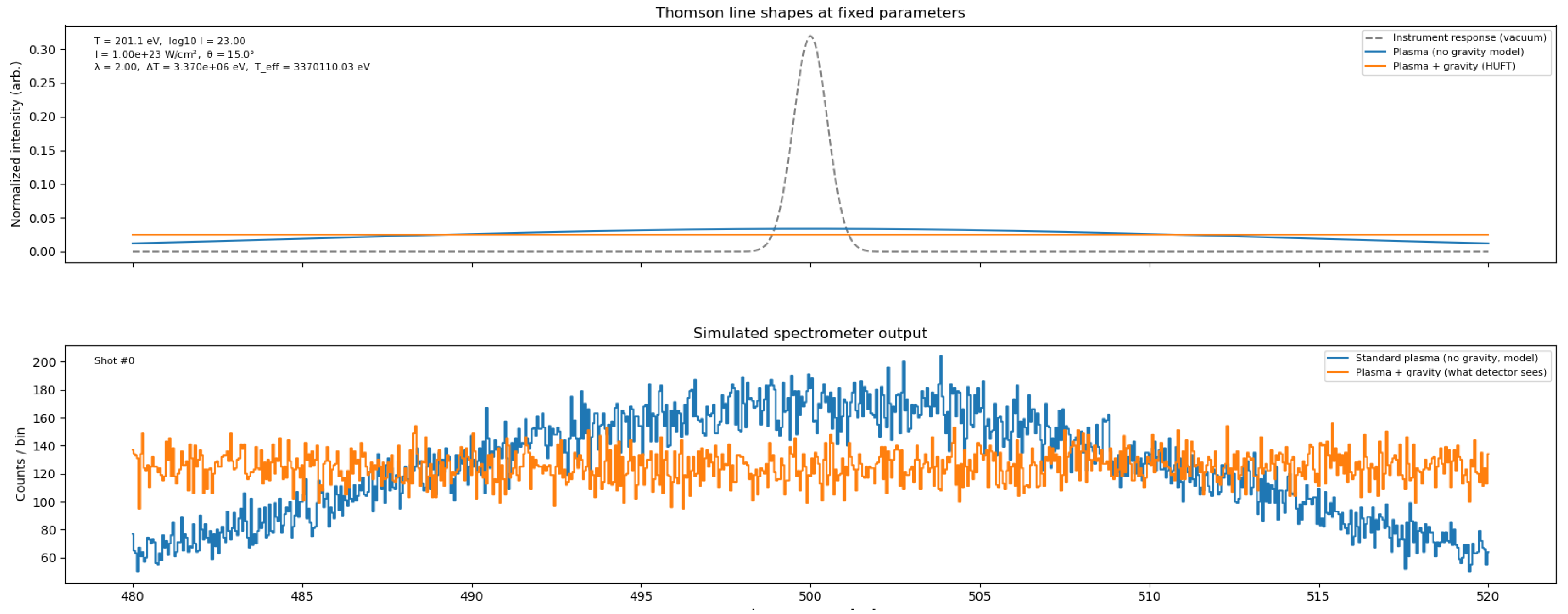
Thomson–scattering simulation used to illustrate the proposed laser–XFEL experiment. Top: Normalized line shapes at fixed parameters. The dashed curve shows the instrumental response measured in vacuum, the blue curve is the standard thermal Thomson line for an underdense plasma (no gravity, local QFT model), and the orange curve includes the additional broadening induced by the effective metric/gravitational correction derived from the equivalence principle. Bottom: Corresponding synthetic spectrometer output in counts per energy bin, including Poisson counting statistics. Both spectra are normalized to the same total counts per shot, so the excess broadening from the gravitational piece appears as a measurable change in the observed line width relative to the standard plasma model.
Figure 2.
Thomson–scattering simulation used to illustrate the proposed laser–XFEL experiment. Top: Normalized line shapes at fixed parameters. The dashed curve shows the instrumental response measured in vacuum, the blue curve is the standard thermal Thomson line for an underdense plasma (no gravity, local QFT model), and the orange curve includes the additional broadening induced by the effective metric/gravitational correction derived from the equivalence principle. Bottom: Corresponding synthetic spectrometer output in counts per energy bin, including Poisson counting statistics. Both spectra are normalized to the same total counts per shot, so the excess broadening from the gravitational piece appears as a measurable change in the observed line width relative to the standard plasma model.
To make the discussion above more concrete, we now illustrate the size of the effect predicted by the effective metric in a parameter regime accessible to forthcoming CPA–XFEL facilities. In Figure 3 we show the theoretical Thomson scattering line shapes for a 500 eV x-ray probe at in three limiting regimes. In vacuum (blue curve) the line is essentially a -function in energy and the observed width is entirely determined by the instrumental resolution. Once the probe traverses a thermal plasma with electron temperature , the dynamical structure factor produces a Gaussian broadening whose width encodes the usual kinetic temperature (orange curve). Including the acceleration-induced effective temperature , leads to an additional broadening (green curve) even though the microscopic plasma temperature T is held fixed; this is the characteristic imprint of the effective non-Minkowski metric in the Thomson spectrum.
Figure 4 isolates this effect by showing the normalized line shape as a function of the optical CPA intensity at fixed geometry and background temperature. Here the only quantity that changes with I is the electron proper acceleration a in the focal region, which enters through. The monotonic growth of the line width with I is therefore a direct, quantitative prediction of the equivalence principle: a stronger non-inertial field (larger a) is locally indistinguishable from a hotter gravitational background and manifests itself as an excess temperature in the Thomson spectrum.
Finally, Figure 5 shows a Monte Carlo realization of what a crystal spectrometer would actually record for the same three regimes. Starting from the theoretical line shapes in Figure 3, we convolve with a realistic instrumental response (FWHM ) and sample the result with Poisson noise to obtain discrete counts per energy bin. In vacuum the signal is dominated by a narrow, instrument-limited spike. The thermal and accelerated plasmas, by contrast, produce broader distributions whose full width at half maximum increases with T and with , respectively. In an experiment one would fit the measured spectra as a function of laser intensity to extract both the baseline kinetic temperature T and the intensity-dependent excess . Detecting a statistically significant, intensity-dependent broadening that cannot be explained by standard plasma effects would constitute direct evidence for the effective metric and, ultimately, for the proposed tabletop probe of quantum gravity.
8. Relativistic Corrections at and Consequences for the Thomson Observable
A convenient measure of whether the electron quiver motion is relativistic is the normalized vector potential:
where and are the peak electric-field amplitude and angular frequency of the optical CPA pulse. Using the standard estimate , one finds that for and m:
In this regime, the magnetic component of the Lorentz force is no longer parametrically suppressed and the full Lorentz force:
must be treated consistently. The usual nonrelativistic estimate no longer applies when the quiver velocity becomes relativistic.
Our primary observable is the Thomson line in the scattered XFEL spectrum, whose width in the accelerated-plasma model can be encoded by an effective temperature . The central assumption in the line-broadening formalism is that the CPA-driven dynamics can be compressed into an effective proper acceleration such as a cycle-averaged ponderomotive acceleration in the focal volume, which then enters the structure-factor broadening.
At ultra-high intensity, however, the same relativistic dynamics that enhance also generically produce a sizeable bulk drift of the electron distribution along the laser propagation direction. Once the electron ensemble acquires a mean drift velocity with , the observed scattered photon energy in the laboratory frame is dominated by Lorentz Doppler kinematics.
For a simple kinematic diagnostic, model the scatterers as having a bulk drift along the direction and assume Thomson scattering is approximately elastic in the instantaneous electron rest frame. Then the detected photon energy may be written schematically as:
where is the incident XFEL photon energy, is the laboratory scattering angle, and D is an angle-dependent Doppler factor. In co-propagating geometry, XFEL along , one finds:
In the ultra-relativistic limit at fixed , this becomes extremely small:
As a result, the Thomson feature can be shifted out of an x-ray spectrometer band. For example, for eV and , a drift as large as implies and hence eV, a near-IR photon energy rather than an x-ray energy.
This shift is not merely a plotting artifact it represents the physical statement that, in co-propagating geometry at sufficiently large , the XFEL photons are chasing a relativistic electron flow, and the lab-frame scattered energy can be strongly redshifted.
If the goal is to measure a small change in the Thomson lineshape attributed to , the co-propagating, ultra-relativistic regime is problematic for three reasons; the out-of-band signal as a conventional soft x-ray spectrometer centered near will register essentially zero counts once is Doppler-shifted to the optical/IR. Extreme sensitivity to drift fluctuations as when , Equation (93) implies that tiny shot-to-shot changes in or in the drift distribution produce order-one changes in and hence in . This induces large apparent broadening and centroid jitter unrelated to the metric-induced . And Competing strong-field emission channels, at , nonlinear Thomson/Compton features and broadband plasma emission become significant backgrounds in the optical/IR, complicating precision inference of a small residual broadening.
There are several concrete strategies to preserve the Thomson-line observable while controlling relativistic systematics such as counter-propagating XFEL geometry; if the XFEL propagates opposite to the mean drift along , the Doppler factor becomes:
which remains for typical angles. This keeps near the x-ray band, restoring compatibility with standard x-ray diagnostics. Operate in the mildly relativistic regime in the probe volume; design the overlap region such that the relevant electrons satisfy such as by probing off-focus, increasing spot size, using shorter , or reducing the effective intensity in the scattering volume, in this regime the magnetic term is again parametrically suppressed and the -based broadening model is more reliable. Small-angle scattering in co-propagation; choosing reduces the redshift; however, it introduces severe background and dynamic-range challenges because the detector must operate close to the unscattered XFEL beam. Drift-suppression modeling for non-free electrons; if plasma physics such as return currents, collisional damping, overdense response suppresses the net bulk drift in the scattering volume, one can parametrize with and a benchmark plane-wave drift . This provides a controlled way to test whether the Thomson feature remains in-band under plausible drift suppression.
A central point that becomes nontrivial at ultra-high intensity is that a fixed-band x-ray spectrometer does not measure a lineshape in the abstract; it measures counts in a finite energy window. In particular, once the CPA-driven electron ensemble develops either a relativistic bulk drift or a very large effective width, the fraction of the scattered signal that actually lies inside a fixed detector band can become parametrically small. In that case, a lineshape difference may exist in principle but be experimentally inaccessible without a compensating increase in photon statistics.
We let denote the normalized probability density for detecting a scattered photon at lab-frame energy E:
A spectrometer with acceptance window records only the fraction:
If denotes the total number of scattered photons entering the spectrometer in a single shot including all energies, then the expected number of in-window counts is:
For binned data with bin width , the expected counts in bin i centered at are:
and we model shot noise by Poisson sampling:
Equations (97)–(100) are the key step that distinguishes an absolute detectability simulation from a purely shape-comparison simulation in which one renormalizes within the window.
Throughout this we take a representative soft x-ray band:
and an incident XFEL photon energy eV at fixed scattering angle . At the CPA pulse can induce a forward drift of the electron distribution along the laser propagation direction. To capture the dominant kinematic effect on the Thomson feature centroid, we model the scatterers as having a mean drift speed along and assume approximately elastic scattering in the instantaneous electron rest frame. The lab-frame centroid of the scattered feature is then taken to be:
with Doppler factor D depending on the relative geometry of probe and drift. For an XFEL co-propagating with the drift:
while for counter-propagation:
Equations (103)–(104) imply that in the ultra-relativistic limit , co-propagation can redshift the scattered feature far below the x-ray band (), whereas counter-propagation keeps .
We parameterize the intrinsic Thomson-feature width by an effective temperature and a Doppler-like width:
which is then convolved with an instrumental resolution: ,
The line model used in the spectrometer simulation is a Gaussian probability density:
The effective metric ingredient enters through a temperature increment so that:
where T is the physical electron temperature or thermal spread in the scattering volume and is the metric acceleration parameter in our phenomenological closure.
Importantly, in this simulation the metric does not modify the scattering kernel from first principles; it enters solely through the broadened , which is precisely the assumption adopted when one maps acceleration curvature effects into an effective temperature in the structure-factor description.
Figure 6 summarizes three benchmark regimes that illustrate the detector-band issue:
- (A)
- Ideal lab baseline: with negligible drift (), hence and . This is the regime in which small changes in width are most readily detectable in a fixed x-ray band.
- (B)
- Realistic with mitigation (counter-prop): with large drift (estimated from a plane-wave radiation-pressure surrogate), but using counter-propagating geometry so that remains near the x-ray band. Even in this case, can be small if becomes very large, in which case large photon statistics (or coarser energy binning) are required.
- (C)
- No mitigation (co-prop): with large drift and co-propagating geometry, giving . Then for a fixed 480–520 eV window and the detector registers essentially zero counts regardless of the intrinsic lineshape.
The top panel of Figure 6 displays the predicted in-window spectral densities for each case for both “flat” () and “metric” () models. The bottom panel displays Poisson-sampled counts using Eqs. (98)–(100). The key point is that even when a metric-induced broadening exists at the level of , its experimental observability is controlled by the capture fraction : if the counts per bin are correspondingly suppressed, and the measurement becomes statistics-limited.
In particular, case (C) demonstrates a band-loss failure mode: the spectrometer window goes dark because the centroid is Doppler-shifted out of band, not because the physics disappears. Case (B) shows that counter-propagation removes the band-loss but can still leave the measurement challenging if the spectrum is too broad in energy, implying that high-throughput collection, multi-shot accumulation, or an instrument with larger acceptance bandwidth is necessary.
At the electron response to the optical drive is generically relativistic (), and the same dynamics that generate large quiver energies also produce a significant net drift from radiation-pressure or ponderomotive drift of the electron ensemble along the laser propagation direction. In that situation, the laboratory-frame position of the Thomson feature is governed not only by the intrinsic plasma broadening and any metric-induced contribution, but also by Doppler kinematics associated with the bulk drift.
To isolate the experimental consequence most relevant to feasibility, we consider a fixed soft x-ray spectrometer window , this is representative of a detector tuned around a XFEL probe. The basic question is for a given geometry at , does the Thomson feature remain inside the detector band with non-negligible photon statistics? If the answer is no, then a small broadening search is moot because the spectrometer simply registers vanishing counts in its operational band.
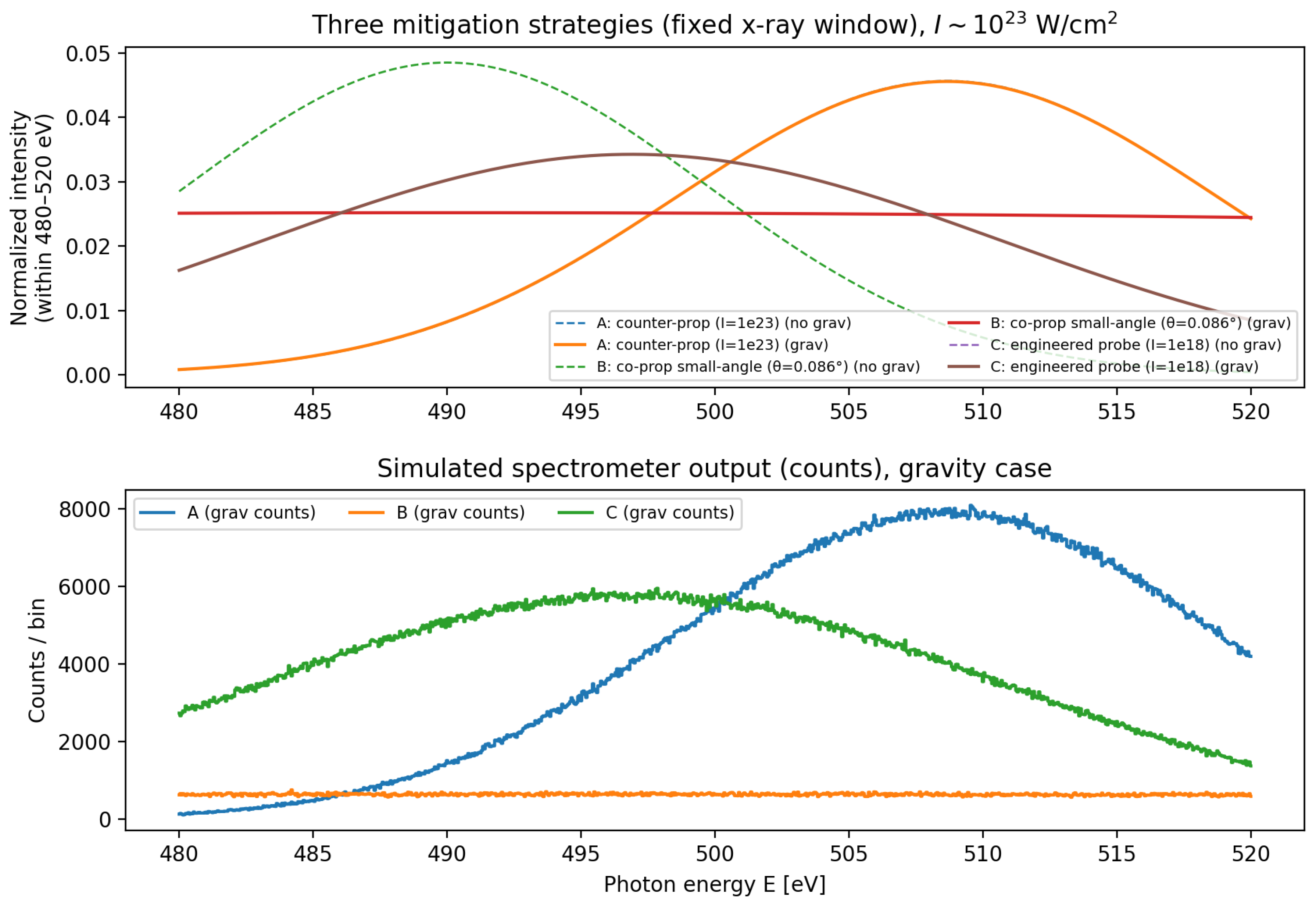
Figure 7 summarizes three concrete mitigation strategies within this fixed-window viewpoint. In all cases we plot (top panel) the predicted in-window line shapes for a baseline plasma model (“no gravity”) and for the metric-modified model (“gravity”), and (bottom panel) a Poisson-realization of the corresponding in-window photon counts for the “gravity” case. The latter is the relevant experimental output as a finite-resolution spectrometer registers binned counts, and if the centroid is Doppler-shifted out of band the expected counts collapse even if the total scattered yield integrated over all energies is large.
In strategy (A) the XFEL propagates opposite to the mean electron drift. In the bulk-drift approximation the kinematic Doppler factor has the schematic form:
which remains for typical scattering angles even when . Consequently the Thomson feature stays near the original x-ray energy scale and therefore remains in-band for a detector centered near . This is reflected in Figure 7: the (A) curves sit well within 480–520 eV, and the bottom-panel counts are large, indicating good statistical visibility. Operationally, counter-propagation is the most robust mitigation because it does not rely on fine-tuning the drift magnitude and it preserves compatibility with standard x-ray diagnostics. In co-propagating geometry the Doppler factor:
can become extremely small when at fixed , leading to strong redshifts of the Thomson feature. One way to reduce this redshift is to enforce (sub-degree scattering). This is the logic of strategy (B): by taking small, the denominator approaches and the redshift is partially mitigated. Figure 7 shows that (B) can indeed keep a feature inside the fixed x-ray window in the model. However, the same small-angle configuration is typically instrumentally demanding as one must collect scattered photons close to the unscattered XFEL beam, which can impose severe dynamic-range, background-rejection, and beam-stop constraints. In the simulated counts (bottom panel), strategy (B) produces substantially fewer in-window counts under the same global normalization, reflecting the practical fact that small-angle collection can be yield-limited once realistic acceptance and background constraints are imposed.
A third approach is to reduce the effective intensity and/or drift in the scattering volume while maintaining a high-intensity drive elsewhere by probing off-focus, increasing spot size in the overlap region, using tailored plasma profiles with return currents, or timing/positioning the probe to sample phases/regions with suppressed net drift. In phenomenological form one may view this as either an intensity reduction in the region interrogated by the XFEL, and/or an effective drift suppression with relative to a plane-wave benchmark . The effect is to keep the Doppler-shifted centroid from migrating out of the detector band. In Figure 7, strategy (C) produces a visible in-window line and substantial in-window counts. The trade-off is that reducing or suppressing drift may reduce the scattered yield and or require additional plasma engineering, but it provides a realistic pathway to keep the Thomson observable in-band while controlling relativistic systematics.
The central lesson of Figure 7 is that at the dominant feasibility constraint for a fixed-band soft x-ray spectrometer is in-band visibility of the Thomson feature. If Doppler kinematics push the centroid out of band, then the detector registers essentially zero counts and one cannot reliably infer small metric-induced changes to the lineshape. Among the strategies considered, counter-propagation (A) is the most robust because it preserves even for large drift; engineered drift/intensity control (C) is a viable secondary path; and small-angle co-propagation (B) can work in principle but is typically limited by instrumental dynamic range and collection geometry.
9. Conclusions
Ultrafast, high-intensity lasers have transformed our ability to generate extreme electromagnetic fields in the laboratory. By exploiting the equivalence between strong acceleration and gravity, these systems effectively realize small, controllable patches of curved or non-inertial space-time in which quantum fields evolve. I have highlighted a particularly promising observable the acceleration- and metric-dependent broadening of x-ray Thomson scattering that can be used to probe quantum mechanics, and ultimately quantum-gravity-inspired effects, in a non-Minkowski background.
In contrast to traditional astrophysical tests of strong gravity, the laser-based approach offers reproducibility, tunability, and the possibility of systematically exploring parameter space. Whether or not quantum gravity leaves an observable imprint at currently accessible accelerations, establishing precision control over quantum phenomena in non-inertial frames will be an important milestone on the path toward a laboratory-based understanding of quantum gravity.
Recent proposals to test quantum gravity via gravity–induced entanglement and decoherence suggest that quantum correlations can be exquisitely sensitive probes of gravitational dynamics [11,12,13,14,16]. In the present context, one could envisage using entangled x–ray photon pairs, with one photon scattered from the accelerated electrons and the other serving as a reference arm. Any acceleration– or metric–dependent decoherence of the two–photon state would provide a complementary observable to simple line broadening, and could in principle distinguish between different classes of nonlocal regulators.
Acknowledgments
I would like to thank my supervisor John. W. Moffat, Professor Donna Strickland for guidance on this project. I would as well like to thank Hilary Carteret, and Arvin Kouroshnia for helpful discussions.
References
- Strickland, D.; Mourou, G. Compression of amplified chirped optical pulses. Opt. Commun. 1985, 56, 219. [Google Scholar] [CrossRef]
- Mourou, G. A. Nobel Lecture: Extreme light physics and application. Rev. Mod. Phys. 2019, 91, 030501. [Google Scholar] [CrossRef]
- Moffat, J. W.; Thompson, E. J. Holomorphic Unified Field Theory of Gravity and the Standard Model. Eur. Phys. J. C [hep-th]. 2025, arXiv:2506.1916185(no.10), 1157. [Google Scholar] [CrossRef]
- Moffat, J. W.; Thompson, E. J. Finite nonlocal holomorphic unified quantum field theory. arXiv 2025, arXiv:2507.14203. [Google Scholar]
- Moffat, J. W.; Thompson, E. J. On the invariant and geometric structure of the holomorphic unified field theory. Axioms 2026, arXiv:2510.0628215(1), 43. [Google Scholar] [CrossRef]
- Moffat, J. W.; Thompson, E. J. On the Standard Model mass spectrum and interactions in the holomorphic unified field theory. arXiv 2025, arXiv:2508.02747. [Google Scholar] [PubMed]
- Moffat, J. W.; Thompson, E. J. Embedding SL(2,C)/Z2 in complex Riemannian geometry. arXiv 2025, arXiv:2506.19158. [Google Scholar]
- Moffat, J. W.; Thompson, E. J. “Comment on a “Comment on `Standard Model Mass Spectrum and Interactions In The Holomorphic Unified Field Theory”. arXiv 2025, arXiv:2508.08510. [Google Scholar] [CrossRef]
- Moffat, J. W.; Thompson, E. J. Gauge-Invariant Entire-Function Regulators and UV Finiteness in Non-Local Quantum Field Theory. arXiv [hep-th. 2025, arXiv:2511.11756. [Google Scholar]
- Moffat, J. W.; Thompson, E. J. On the Complexified Spacetime Manifold Mapping of AdS to dS. arXiv [gr-qc]. 2025, arXiv:2511.11658. [Google Scholar]
- Bose, S. , Spin entanglement witness for quantum gravity. Phys. Rev. Lett. [gr-qc]. 2017, arXiv:1707.06050119, 240401. [Google Scholar] [CrossRef]
- Marletto, C.; Vedral, V. Gravitationally induced entanglement between two massive particles is sufficient evidence of quantum effects in gravity. Phys. Rev. Lett. [quant-ph]. 2017, arXiv:1707.06036119, 240402. [Google Scholar] [CrossRef]
- Krisnanda, T.; Tham, G. Y.; Paternostro, M.; Paterek, T. Observable quantum entanglement due to gravity. npj Quantum Inf. 6 [quant-ph]. 2020, arXiv:1906.0880812. [Google Scholar] [CrossRef]
- Carteret, H. A. Estimating the entanglement negativity from low-order moments of the partially transposed density matrix. arXiv [quant-ph. arXiv:1605.08751. [CrossRef]
- Anwar, M. S. , Implementation of NMR quantum computation with para-hydrogen derived high purity quantum states. Phys. Rev. A 2004, arXiv:quant70, 032324. [Google Scholar] [CrossRef]
- Anwar, M. S. , Practical implementations of twirl operations. Phys. Rev. A 2005, arXiv:quant71, 032327. [Google Scholar] [CrossRef]
- Birrell, N. D.; Davies, P. C. W. Quantum Fields in Curved Space; Cambridge University Press: Cambridge, 1982. [Google Scholar]
- Crispino, L. C. B.; Higuchi, A.; Matsas, G. E. A. The Unruh effect and its applications. Rev. Mod. Phys. [gr-qc]. 2008, arXiv:0710.537380, 787. [Google Scholar] [CrossRef]
- Chen, P.; Tajima, T. Testing Unruh radiation with ultraintense lasers. Phys. Rev. Lett. 1999, 83, 256. [Google Scholar] [CrossRef]
- Gregori, G. A laboratory model of post-Newtonian gravity with high power lasers and 4th generation light sources. Class. Quantum Grav. 2016, 33 075010. [Google Scholar] [CrossRef]
- Gregori, G. Measuring Unruh radiation from accelerated electrons. arXiv 2023, arXiv:2301.06772. [Google Scholar] [CrossRef]
- Crowley, B. J. B. Testing quantum mechanics in non-Minkowski space-time with high power lasers and 4th generation light sources. Scientific Reports 2012, 2, 491. [Google Scholar] [CrossRef]
- Moffat, J. W. Ultraviolet complete quantum gravity. Eur. Phys. J. Plus 2011, arXiv:1008.2482126, 43. [Google Scholar] [CrossRef]
- Moffat, J. W. Quantum gravity and the cosmological constant problem. arXiv 2014, arXiv:1407.2086. [Google Scholar] [CrossRef]
- Tomboulis, E. T. hep-th/9702146; Superrenormalizable Gauge and Gravitational Theories. 1997.
- Biswas, T.; Gerwick, E.; Koivisto, T.; Mazumdar, A. Towards Singularity- and Ghost-Free Theories of Gravity. Phys. Rev. Lett. 2012, 108, 031101. [Google Scholar] [CrossRef]
- Talaganis, S.; Biswas, T.; Mazumdar, A. Towards Understanding the Ultraviolet Behavior of Quantum Loops in Infinite-Derivative Theories of Gravity. Class. Quant. Grav. 2015, 32, 215017. [Google Scholar] [CrossRef]
- Buoninfante, L.; Lambiase, G.; Mazumdar, A. Ghost-Free Infinite Derivative Quantum Field Theory. Nucl. Phys. B 2019, 944, 114646. [Google Scholar] [CrossRef]
- Landry, R.; Moffat, J. W. Nonlocal Quantum Field Theory and Quantum Entanglement. Eur. Phys. J. Plus 139 [hep-th]. 2024, arXiv:2309.06576v371. [Google Scholar] [CrossRef]
- Evens, D.; Moffat, J. W.; Kleppe, G.; Woodard, R. Nonlocal regularizations of gauge theories. Phys. Rev. D 1991, 43, 499. [Google Scholar] [CrossRef] [PubMed]
- Efimov, G. V. Non-local Quantum Theory of the Scalar Field”. Commun. Math. Phys. 1967, 5, 42. [Google Scholar] [CrossRef]
- Kleppe, G.; Woodard, R. P. “Nonlocal Yang-Mills”. Nucl. Phys. [hep-th. 1992, arXiv:9203016v1B388, 81–112. [Google Scholar] [CrossRef]
- Moffat, J. W. “Ultraviolet Complete Quantum Field Theory and Gauge Invariance”. arXiv [hep-th. arXiv:1104.5706. [CrossRef]
- Moffat, J. W. “Ultraviolet Complete Quantum Field Theory and Particle Model”. Eur. Phys. J. Plus 2019, arXiv:1812.01986v4134, 443. [Google Scholar] [CrossRef]
- Moffat, J. W. “Model of Boson and Fermion Particle Masses”. Eur. Phys. J. Plus [hep-ph. 2021, arXiv:2009.10145v2136, 601. [Google Scholar] [CrossRef]
- Green, M. A.; Moffat, J. W. “Finite Quantum Field Theory and the Renormalization Group”. Eur. Phys. J. Plus [hep-th]. 2021, arXiv:2012.04487136, 919. [Google Scholar] [CrossRef]
- Moffat, J. W. Proc. of the 1st Karl Schwarzschild Meeting on Gravitational Physics; Springer, 2016; p. 229. [Google Scholar]
- Peskin, M. E.; Schroeder, D. V. “An Introduction to Quantum Field Theory”; Perseus Books; quant-th, 1995. [Google Scholar]
- Modesto, L.; Moffat, J. W.; Nicolini, P. Black holes in an ultraviolet complete quantum gravity. Physics Letters B [gr-qc]. 2011, arXiv:1010.0680v3695. [Google Scholar] [CrossRef]
- Carteret, H. A. Noiseless quantum circuits for the Peres separability criterion. Phys. Rev. Lett. 2005, arXiv:quant94, 040502. [Google Scholar] [CrossRef] [PubMed]
- Carteret, H. A. Exact interferometers for the concurrence and residual 3-tangle. arXiv 2003, arXiv:quant. [Google Scholar]
- Alebastrov, V.A.; Efimov, G.V. A proof of the unitarity of S-matrix in a nonlocal quantum field theory. Commun. Math. Phys. 1973, 31, 1–24. [Google Scholar] [CrossRef]
- Fedotov, A. M. Advances in QED with intense background fields. Phys. Rep. 2022, 1010, 1–138. [Google Scholar] [CrossRef]
- Lei, B.; Zhang, H.; Seipt, D.; Bonatto, A.; Qiao, B.; Resta-López, J.; Xia, G.; Welsch, C. P. Coherent synchrotron radiation by excitation of surface plasmon polariton on near-critical solid microtube surface. arXiv [physics.acc-ph. 2025, arXiv:2507.04561. [Google Scholar] [CrossRef]
- Welsch, C. P. “Tabletop particle accelerator could transform medicine and materials science,”. The Conversation 2025. [Google Scholar]
- Welsch, C. P. A radical new kind of particle accelerator could transform science. ScienceAlert 2025. [Google Scholar]
Figure 3.
Theoretical Thomson scattering line shapes for a 500 eV x-ray probe at scattering angle . The blue curve shows the nearly -function line expected in vacuum, broadened only by the assumed instrumental response. The orange curve corresponds to a thermal plasma with electron temperature . The green curve shows the prediction including the acceleration-induced effective temperature obtained from the variable-mass metric, which produces additional broadening beyond the purely thermal width. All curves are normalized to unit area.
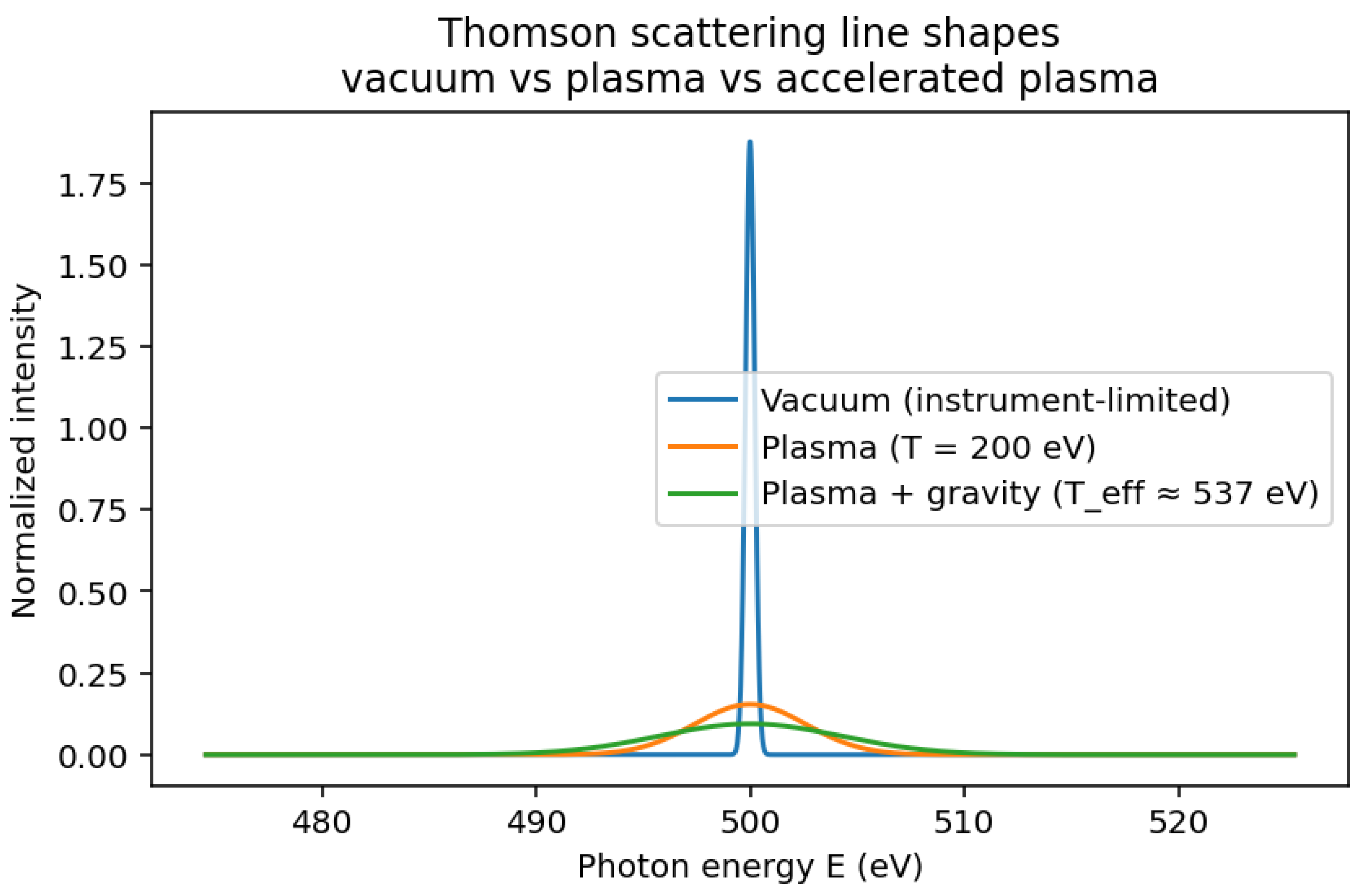
Figure 4.
Acceleration-induced broadening of the Thomson line as a function of the optical CPA intensity. We fix the probe photon energy at , the scattering angle at , and the background plasma temperature at , and vary the laser intensity between . Increasing I increases the proper acceleration a of electrons in the focus, which in turn increases the effective temperature and hence the Gaussian width . Each curve is normalized to unit peak height to highlight the systematic growth of the line width with intensity, which is the key signature of the gravitational (equivalence principle) contribution.
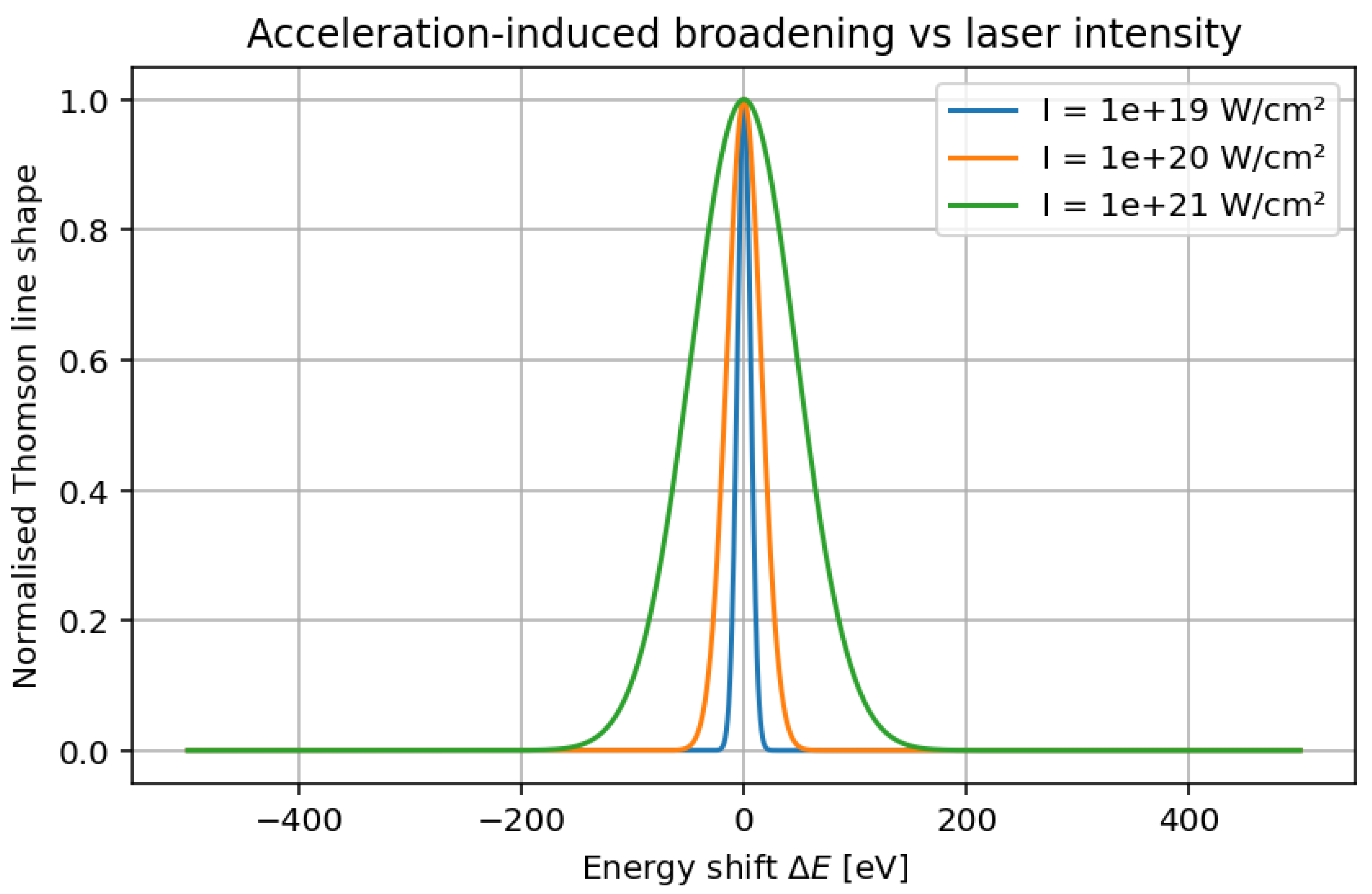
Figure 5.
Monte Carlo simulation of what a crystal spectrometer would record in a single shot for the three regimes in Figure 3: vacuum (blue), thermal plasma at (orange), and accelerated plasma with (green). The continuous theoretical line shapes are convolved with a finite instrument response (Full Width at Half Maximum (FWHM) ) and sampled with Poisson noise to obtain discrete counts per energy bin. In vacuum the line is instrument-limited and appears as a narrow spike, while the thermal and accelerated plasmas produce successively broader distributions. Fitting the measured widths as a function of laser intensity allows one to extract T and separately and thereby isolate the acceleration-dependent excess temperature .
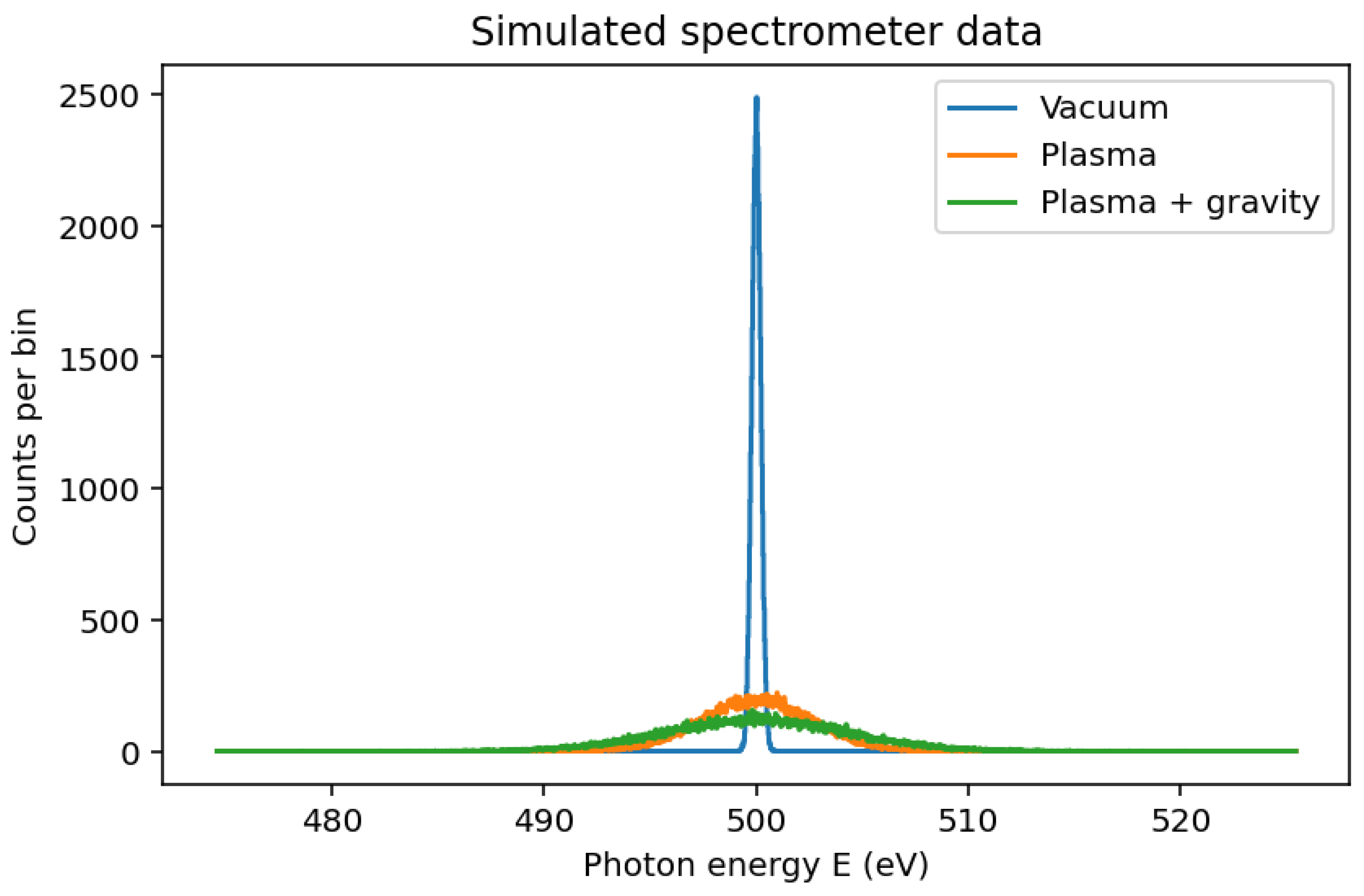
Figure 6.
Three benchmark scenarios in a fixed 480–520 eV x-ray spectrometer window at and eV. Top: predicted in-window spectral densities for a “flat” model. Bottom: Poisson-sampled counts using the absolute window fraction.
Figure 6.
Three benchmark scenarios in a fixed 480–520 eV x-ray spectrometer window at and eV. Top: predicted in-window spectral densities for a “flat” model. Bottom: Poisson-sampled counts using the absolute window fraction.
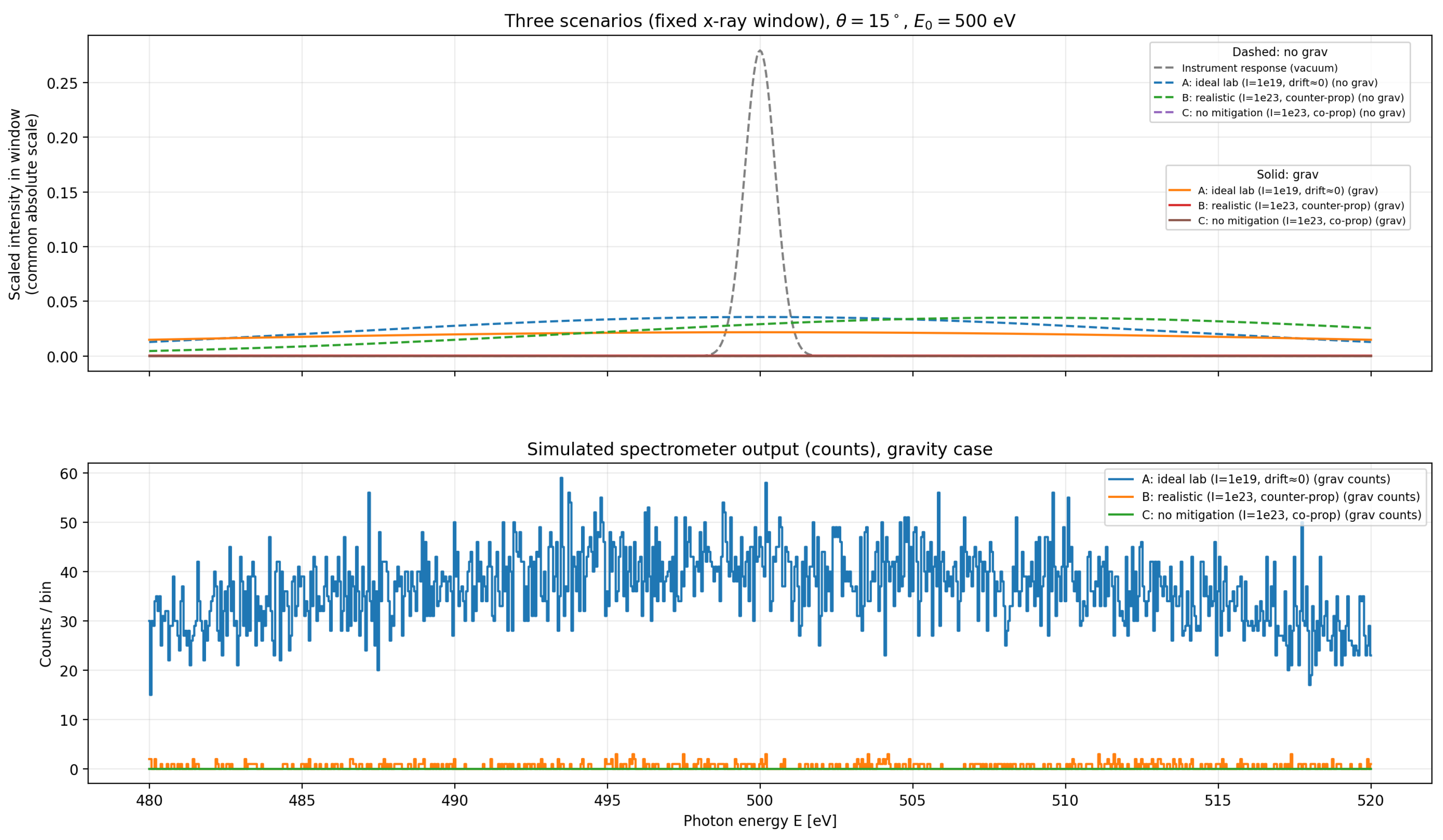
Figure 7.
Three mitigation strategies for maintaining Thomson-feature visibility in a fixed soft x-ray spectrometer window at . Top: predicted in-window line shapes (dashed: baseline model, solid: metric-modified model). Bottom: simulated binned photon counts (Poisson noise) in the same window for the metric-modified case. The dominant feasibility criterion at ultra-high intensity is whether Doppler drift kinematics keep the Thomson feature in-band with sufficient photon statistics for a “small broadening” measurement.
Disclaimer/Publisher’s Note: The statements, opinions and data contained in all publications are solely those of the individual author(s) and contributor(s) and not of MDPI and/or the editor(s). MDPI and/or the editor(s) disclaim responsibility for any injury to people or property resulting from any ideas, methods, instructions or products referred to in the content. |
© 2025 by the author. Licensee MDPI, Basel, Switzerland. This article is an open access article distributed under the terms and conditions of the Creative Commons Attribution (CC BY) license.
Copyright: This open access article is published under a Creative Commons CC BY 4.0 license, which permit the free download, distribution, and reuse, provided that the author and preprint are cited in any reuse.


