
Submitted:
22 January 2026
Posted:
23 January 2026
You are already at the latest version
Abstract
This paper presents probabilistic wind energy forecasting using quantile regression averaging combined with a conformal prediction modelling framework. The study uses data from Eskom, South Africa's power utility company. The data is from April 2019 to November 2023. A partial linear additive quantile regression (PLQR) averaging method is used to combine forecasts from two competing forecasting models: eXtreme Gradient Boosting (XGBoost) and Principal Component Regression (PCR). To compare the predictive abilities of the models, two data splits are used: 80\%, 10\% and 10\% for the first set, and 85\%, 10\% and 5\% for the second set. Empirical results suggest that the combined predictions from PLAQR perform better than the individual models, significantly improving calibration and accuracy. The proposed combination has the smallest root mean square error (RMSE) and the highest probability of change in direction (POCID). The combination captures nonlinearities and produces well-calibrated probabilistic results. Probability integral transform histograms validate this. This performance gain reflected the importance of data volume. This is reinforced by the fact that the PLAQR model, which combines the benefits of tree-based approaches and linear models, is a robust modelling approach for reliable renewable energy forecasting. Future research directions should consider more varied ensembles.
Keywords:
conformal prediction
; model calibration
; probabilistic forecasting
; quantile regression averaging
; wind energy
1. Introduction
1.1. Overview
Among the renewable energies, wind power stands out, and getting its short-term forecasts right is crucial to the smooth management of energy. Techniques from machine learning, such as Extreme Gradient Boosting (XGBoost), have increased the accuracy of wind forecast models in capturing the intricate behaviour of wind energy. However, measuring how good those forecasts are remains challenging. Conformal prediction offers a solution by pairing a precise point forecast with an accompanying prediction interval that quantifies uncertainty. In this work, we present a hybrid approach to improve the accuracy and reliability of wind energy forecasts by combining XGBoost with conformal prediction.
1.2. Literature Review
Wind power is one of the major contributors to global renewable power generation [1]. However, the unpredictability of wind power has been identified as a challenge for power grid management [2]. The production of power by wind is influenced by wind resources such as wind speed, which vary both spatially and temporally [2]. Short-term wind power forecasting, which involves predicting wind power output over a time interval of a few minutes to a few days [3], has become necessary for effective power grid management [2]. The increase in the unpredictability of power management is also attributed to the increase in the number of power resources [4].
Accurate predictions help reduce costs, improve accuracy, and optimise decision-making for investments in renewable energy resources [5]. Even with advanced forecasting models, inaccuracies persist, mainly due to the complexity of wind. The high levels of uncertainty and chaotic behaviour associated with wind speed variations make achieving high accuracy difficult. This paper proposes using the XGBoost model for short-term wind energy predictions, compared with Principal Component Regression, and incorporates conformal prediction.
1.2.1. Wind Energy Forecasting: Methods and Challenges
Statistical approaches such as the AutoRegressive Integrated Moving Average (ARIMA) and Persistence Models are widely employed for wind power forecasting [6]. However, these approaches tend to struggle with the non-linear relationship between wind power and weather variables. In response to these issues, new approaches based on ensemble forecasting have emerged that consider both temporal and geographical ensembles [2]. These approaches combine autoregression, integration, and moving-average models with variables, as well as polynomial regression with time series data, to enable probabilistic forecasting.
Machine learning algorithms, such as Artificial Neural Networks (ANNs) and Support Vector Machines (SVMs), have demonstrated their effectiveness in modelling non-linear processes [7]. Recent comparative analysis shows that several machine learning algorithms, like ANN, Random Forest (RF),XGBoost, K-Nearest Neighbours (KNN), and Multi-Layer Perceptron Artificial Neural Network (MLP ANN), have been able to produce more accurate results than traditional models [5].
Ensemble approaches such as Random Forests and Gradient Boosting Machines have attracted interest for their ability to provide robust and accurate predictions. Stacking ensemble methods, which use multiple models as base models for prediction, have been observed to perform significantly better than the individual models when XGBoost, SVM with a linear kernel, MLP Classifier, and KNN are compared. However, the challenges posed by wind power prediction uncertainties must be overcome for effective decision-making. The variability of wind energy sources underscores the importance of wind power forecasting to ensure grid stability and security [8].
1.2.2. XGBoost for Wind Energy Forecasting
XGBoost, a gradient-boosting library, was developed by [9] and has become a prominent algorithm with improved efficiency and performance. XGBoost has gained popularity as a top machine learning algorithm because it can efficiently handle large volumes of data, missing values, and overfitting problems through regularisation techniques. In wind energy prediction, XGBoost has been successfully applied to predict wind speed and power output across various applications and regions.
Numerous comparative studies have emphasised the effectiveness of XGBoost in wind power prediction. For example, in a short-term wind power prediction task, the authors of [10] proposed a novel XGBoost technique with a hyperparameter search technique based on the Bayesian approach (BH-XGBoost), and the results showed that the performance of the BH-XGBoost model surpassed XGBoost, SVM, KELM, and LSTM in all test conditions. It performed well in wind ramp situations, including extreme weather, and in low-wind-speed conditions.
Similarly, [11] conducted detailed comparisons of XGBoost against Support Vector Regression (SVR), Gaussian Process Regression (GPR), and Neural Networks (NN). The study’s results showed that the XGBoost model was the most effective, particularly for short-term predictions. In a separate study [12], random forests were used for hour-ahead wind power forecasting, with results showing accurate forecasts.
Zheng et al. [4] introduced a novel hybrid model that integrates XGBoost with LSTM networks and technical analysis indicators such as the KDJ, Stochastic Oscillator, and MACD, achieving a normalised mean absolute error of 0.0396 for wind power forecasting with a processing time of about 550 seconds. In a comparative analysis, Ref [13] compared the performance of Convolutional Neural Network and Gated Reccurrent Unit (CNN GRU) models with XGBoost and Random Forest models, indicating that while deep learning models can perform better, XGBoost is still a strong competitor in day-ahead wind power forecasting tasks. Recent studies have also demonstrated the efficacy of XGBoost for energy consumption forecasting, including solar power, and its growing use in wind power forecasting. Ahmed et al. [14] introduced an integrated boosting method (Boost-LR) that combines XGBoost, CatBoost, and Random Forest with Linear Regression, achieving improvements of 31.42%, 32.14%, and 27.55% in mean absolute error over individual models on different wind farm datasets.
1.2.3. Principal Component Regression
Principal Component Regression (PCR) is a method that combines PCA with Multiple Linear Regression to eliminate multicollinearity among predictor variables. The technique helps convert a set of correlated variables into fewer uncorrelated variables, thereby increasing the model’s stability. The PCR helps to simplify the regression model structure by reducing overfitting [15].
Although this is a linear technique, it works well even when predictors are correlated, a common situation in meteorological datasets used to predict wind energy. However, there is a significant gap in the literature regarding the use of PCR for wind energy predictions, both in comparison with other models and in general. Some meteorological datasets that can be used to predict wind energy may be correlated, including, but not limited to, temperature, pressure, and humidity. There are no applications or comparisons that can be made in the context of using PCR to predict wind energy.
1.2.4. Hyperparameter Optimisation
The performance of XGBoost is highly dependent on hyperparameter optimisation. Ref [10] suggests an optimised XGBoost model for short-term wind power forecasting, proving that Bayesian optimisation improves the accuracy of predictions over grid search. Their BH-XGBoost model performed better in various wind farm scenarios, achieving lower estimated errors than the conventional method and performing well in wind ramp situations and harsh weather conditions.
In a similar vein, the importance of hyperparameter optimisation for improving model performance is also highlighted in [16]. Advanced optimisation algorithms have also been coupled with feature engineering techniques.
Zheng et al. [4] integrated hyperparameter optimisation with technical indicator improvement, using financial market indicators such as the Stochastic Oscillator (SO) and Moving Average Convergence and Divergence (MACD), thereby enhancing ultra-short-term wind power forecast accuracy. The need for systematic hyperparameter optimisation is not only relevant for varying model parameters but also for advanced model improvement techniques. Bayesian optimisation is a tactical approach to exploring the complex hyperparameter space of XGBoost. It is essential for obtaining reliable, accurate wind power forecasts, which are critical for handling difficult forecast conditions.
1.2.5. Traditional Methods vs. Machine Learning Methods in Wind Energy Forecasting
Recent studies have shown that machine learning algorithms outperform traditional statistical models for wind energy prediction. Traditional models such as ARIMA and SARIMA have been used for benchmarking purposes because of their simplicity. However, these models have the disadvantage of assuming linearity and stationarity, which limits their effectiveness in dealing with the nonlinear nature of wind energy.
Liu et al. [17] believe that machine learning algorithms, such as XGBoost, Random Forest, and LSTM, outperform traditional algorithms in learning complex patterns in the data and responding to the dynamics in wind data. Their superiority has been consistently demonstrated in comparison studies. For example, in Ref [8], the best normalised mean absolute error (NMAE) of 5.15% was obtained by gradient boosting machine (GBM) algorithms in short-term forecasting models using 15-minute interval time series data, outperforming traditional algorithms.
In addition, [5] conducted comprehensive comparisons of machine learning techniques, showing that XGBoost and Random Forest outperformed traditional statistical methods in terms of stability and accuracy for medium- and long-term forecasts. The authors emphasised the efficiency of machine learning methods for processing the complex, nonlinear relationships inherent in wind power generation data.
Ponkumar et al. [18] tested various machine learning algorithms, including LightGBM, Random Forest, CatBoost, and XGBoost, for very short-term forecasting. The results revealed that these advanced methods consistently outperformed conventional statistical models across mean absolute error (MAE), mean squared error (MSE), root mean squared error (RMSE), and R-squared.
1.2.6. Uncertainty Quantification and Conformal Prediction
Although the performance of XGBoost and other models has been impressive in terms of predictive accuracy, they have been limited to point predictions, which do not provide information about prediction uncertainty. This can cause suboptimal operational decisions in energy management. The literature shows a significant research gap in uncertainty estimation techniques for wind power forecasting, and recent studies have mainly focused on improving the accuracy of point predictions rather than estimating uncertainty. Conformal prediction, introduced by [19] and further improved by [20], provides a statistically sound approach to constructing prediction intervals that guarantee containing predictions with a specified confidence level. Recent studies by [21] have shown that the combination of conformal prediction and machine learning models enables the estimation of quantifiable uncertainty. Although [2] addressed probabilistic forecasting using improved ensemble methods and analogue ensemble methods to decrease uncertainty, demonstrating that probabilistic forecasting can assist grid managers in determining the most important time points for grid operation and preparing for problems caused by wind power variability, the application of conformal prediction to wind energy forecasting has not been investigated yet.
The state of the art in uncertainty qunatiication is not optimal. For example, the study in [13] conducted statistical validation using the Diebold-Mariano test, showing significant differences in performance, but the current state of the art is grounded in statistical hypothesis testing rather than uncertainty quantification for operational forecasting. A stronger paradigm is needed in wind forecasting, where not only accuracy but also forecast reliability, with probabilistic confidence limits on the output, are of utmost importance.
The integration of XGBoost and conformal prediction remains an unexplored area in wind energy forecasting. This research aims to bridge a gap in the literature by developing a framework that produces accurate point forecasts and proper uncertainty intervals, thereby addressing the primary requirement for uncertainty-aware forecasts in power management systems.
1.3. Contribution and Research Highlights
The PLAQR Ensemble Method, integrating XGBoost with PCR, yields better-calibrated predictions with greater accuracy in the context of conformal prediction, making it an efficient method for renewable energy forecasting.
The key findings of this research are as follows:
- In the conformal prediction framework, PLAQR ensures correctly calibrated probabilistic forecasts, confirmed through PIT histograms, and thus represents an improvement in the integration of accuracy and probability forecast estimation.
- This is achieved by the use of nonlinearities, together with tree and linear approaches, which give a higher directional accuracy (POCID) and a lower error (RMSE) than the other models.
- The more the data in the training dataset, the better the performance (85% vs. 80%). This shows the significance of data size when building data-driven models for predicting wind energy.
- This approach provides a template for developing successful prediction models in renewable energy, where reliable uncertainty estimation is of prime importance.
2. Models
The modelling framework proposed in this study is given in Figure 1. The flowchart illustrates a general forecasting system. Preprocessing and feature engineering are applied to the input time series data. Two models are trained and tuned: XGBoost, which is the primary model, and Principal Component Regression (PCR), the benchmarking model. The forecasted points are validated by metrics such as RMSE, MAE, and MASE. Another path within the system concerns the measurement of prediction intervals via conformal prediction and is validated using metrics such as PICP and MPIW. Both forecast points and intervals are produced with complete validation.
2.1. eXtreme Gradient Boosting
eXtreme Gradient Boosting (XGBoost) was introduced by Tianqi Chen and Carlos Guestrin in 2016 [22]. It builds on gradient boosting [23]. XGBoost is a highly scalable and efficient algorithm for gradient boosting [24]. Gradient boosting is an ensemble learning technique that constructs multiple decision trees in a sequential manner. Each new tree is trained to predict the errors (residuals) made by the previous trees, which allows for iterative improvements in overall prediction accuracy. This process results in the creation of a strong predictive model.
The key principles of gradient boosting are as follows:
2.1.1. Additive Learning
Additive learning in XGBoost is a boosting ensemble technique where the predictive model is built iteratively. This process involves sequentially adding new decision trees to an already trained ensemble. In Xgboost ensemble methods, additive learning builds the final prediction model gradually. It starts with an initial model, and in each iteration, a new weak learner is trained to address the errors of the ensemble . This weak learner is then added to the ensemble, leading to an improved overall model.
2.1.2. Loss Function
The loss function is the difference between the predicted values and the actual values. XGBoost has been shown to handle a large number of different loss functions, depending on the type of problem being tackled. The loss function in regression problems is the Mean Squared Error, given in Equation (2).
where is the actual values and is the predicted values.
2.1.3. Regularisation
Regularisation is a crucial set of techniques to prevent the model from overfitting the training data. XGBoost incorporates a regularisation term, , into its overall objective function . The objective function aims to minimise both the prediction error (measured by the loss function, and the model complexity measured by the regularisation term. The equation is as follows:
The specific form of the regularisation term used here is
where T is the number of leaf nodes, and w is the weight of the tree, which specifies the complexity of the tree, that is, , and are the parameters controlling complexity. The larger the value, the more complex the structure of the tree.
By adding this regularisation term to the objective function, XGBoost does not just try to minimise the error on the training data; it also tries to build an inherently simpler and more generalisable model.
Rather than fitting the entire model at once, we optimise it iteratively. We begin with an initial prediction . At each step, we add a new tree to enhance the model. The updated prediction after adding the tree can be expressed as follows:
In decision trees, Boosting is used during the model’s training to minimise the objective function. This technique involves adding a new function f to the existing model iteratively. Therefore, in the iteration, a new function is added as follows:
The algorithm can also handle missing data and make precise decisions on where to split data based on gains. Further, XGBoost relies on post-pruning for improving efficiency. It is well-known for its scalability and flexibility, making it one of the most favourable algorithms for handling big data. Though XGBoost has many advantages over other learning algorithms, its parameters must be carefully tuned for better performance [16].
2.2. Principal Component Regression
Principal component regression(PCR) is a benchmark model in this study. It is a dimension reduction technique that is useful when multicollinearity exists among the explanatory variables in the multiple regression framework. A standard multiple linear regression model is defined as :
where Y represents the vector of observed values, X denotes a matrix of explanatory variables, indicates the parameter vector, and signifies the vector of error terms. The least squares solution for estimating the parameter is expressed as follows:
When multicollinearity is present, may be singular, resulting in unstable coefficient estimates with higher variance. PCR changes the original matrix into lower dimensional orthogonal space using Singular Value Decomposition (SVD) to solve this issue.
To get our first m principal components, we use SVD to approximate the X matrix:
where T represents orthogonal scores, while P denotes loadings. Both U and V are orthonormal, and the matrix D is diagonal with positive real entries. Consequently, regressing Y on the scores results in:
2.3. Evaluation Metrics
Evaluation metrics are essential in determining the ability of forecasting methods to predict the future of time series data. We discuss in the subsequent sections some of the performance evaluation metrics.
2.3.1. Root Mean Square Error
The root mean square error (RMSE) is the average of the squared differences between the predicted and actual values, indicating how well the model’s predictions fit the actual data. The RMSE is calculated using Equation (11).
where is the actual value, denotes the predicted value of the observation and m represents the total number of predictions. A lower RMSE value indicates that the predictions are closer to the actual data points, indicating better model performance.
2.3.2. Mean Absolute Error
2.3.3. Mean Absolute Scaled Error
The mean absolute scaled error (MASE) is a forecast evaluation metric used to evaluate forecasts’ accuracy, especially in time series analysis. It compares the forecast errors to those of a naive benchmark model. For a seasonal time series, the MASE is defined by Equation (13).
where , and m are as defined in Equation (11) and denotes the predicted value of the observation. A low MASE value is desirable as it indicates better predictive performance.
2.3.4. Mean Bias Error
2.3.5. Prediction of Change in Direction
A major disadvantage of using evaluation metrics such as RMSE, MAE, MASE, and MBE is that they do not account for changes in forecast direction. This drawback is overcome by using the prediction of change in direction (POCID), which counts the number of correct direction changes [25]. The POCID is calculated using Equation (15).
where m is the total number of forecasted periods, is a directional indicator function for time period t, defined as:
The condition checks if the predicted and actual movements have the same sign. The actual change is denoted by , while is the predicted change. If the product is positive, both changes are in the same direction (both positive or both negative), and the prediction is counted as correct (). However, if the product is zero or negative, the directions did not match, and the prediction is counted as incorrect ().
A major drawback of POCID is that it does not consider the closeness of the predictions to the actual values. In their study [25], they developed a fitness metric. This metric combines POCID and MSE [25]. In this study, we extend the fitness metric by using a data-driven weight, w and RMSE. The modified fitness metric is given in Equation (16).
where w is calculated as follows
with k representing the number of models. Therefore
Higher values of the Fitness metric indicate better model performance in predicting fluctuations and greater prediction accuracy.
2.4. Conformal Predictions
Conformal Prediction (CP) is a non-parametric statistical approach developed for reliable uncertainty estimation in machine learning models [26]. The main advantage of CP is its ability to produce prediction sets or intervals that provide finite-sample marginal coverage guarantees. Crucially, it does so without making strong assumptions about the underlying data distribution or the model errors.
The main goal of CP is to produce a prediction set for a new input such that the corresponding true response belongs to the set with a probability no less than a confidence level of . This is to ensure that the validity condition expressed in Equation (18) is satisfied.
2.5. Prediction Interval Evaluation Metrics
2.5.1. Prediction Interval Coverage Probability)
The Prediction Interval Coverage Probability (PICP) evaluation metric calculates the percentage of actual observations that lie within their corresponding predicted intervals. It is the key measure of the validity or reliability of an interval [27]. The formula for PICP is expressed as in Equation (19).
where is the actual value of the observation, is the prediction interval with lower bound and upper bound for that observation, and m is the total number of observations.
2.5.2. Mean Prediction Interval Width)
The Mean Prediction Interval Width (MPIW) measures the average width of the prediction intervals, which quantifies their sharpness or precision. A narrower interval is more informative, provided it maintains valid coverage [27]. The formula for MPIW is given by:
where and are the upper and lower bounds of the prediction interval for the observation, and m is the number of observations. A lower MPIW is desirable, but it should only be used to compare models that have already achieved a valid PICP.
2.5.3. Coverage Width-Based Criterion)
The Coverage Width-based Criterion (CWC) is a score that penalises both low coverage and large interval widths. It provides a single value to be minimised [27]. One common formulation is:
where is the nominal coverage rate, is an indicator function and is a scaling parameter that controls how heavily under-coverage is penalised.
2.5.4. Probability Integral Transform (PIT) Histogram
The PIT is a graphical method for evaluating the probabilistic calibration of an entire predictive distribution, not just a single interval. It is calculated by applying the forecasted Cumulative Distribution Function (CDF) to its corresponding actual observation [28].
where is the actual value of the observation and is the forecasted CDF for that observation. The resulting set of values is then plotted as a histogram. For a perfectly calibrated forecast, the values should be uniformly distributed on , resulting in a flat histogram.
3. Results
3.1. Exploratory Data Analysis
3.1.1. Data Source
This study utilises wind energy data sourced from Eskom, South Africa’s power utility company. This data is freely available and can be accessed at https://www.eskom.co.za/dataportal/. The data covers the period from 02 April 2019 to 28 November 2023.
3.1.2. Data Characteristics
The data will be split into two different sets of splits which are (80% training test, 10% validation and 10% test) and (85% training test, 10% validation and 5% test). The response variable in this study is Wind energy produced, for which we are going to do predictions. The explanatory variable on the dataset are as follows:
- difLag1 is the first-order hourly difference in the Wind energy produced time series:
- difLag2 is the second-order hourly difference in the Wind energy produced time series:
- difLag12 is the difference from half a day prior:
- difLag24 is the daily seasonal difference :
- Hour is representing the hour of the day (0 to 23).
- Day is representing the day of the week.
- noltrend is the estimated non-linear trend component of the wind energy produced time series. This component was extracted through Seasonal and Trend decomposition using Loess
Figure 2 below display distribution of eight histograms showing different patterns in various variables. Day and Hour have uniform distributions, while difLag1, difLag2, difLag12, and difLag24 show bell-shaped distributions centred around zero, showing small lagged differences. In contrast, noltrend and Wind exhibit right-skewed distributions with more lower values and fewer higher values..
3.1.3. Summary Statistics
Table 1 shows the summary statistics for wind energy production from 2 April 2019 until 27 November 2023. The data has a minimum wind energy produced is 19.8 and a maximum of 3102.2 for the specified period. The central tendency shows the median of 903.0 and a mean of 982.5, which are closer to each other, suggesting that the distribution is moderately right-skewed, with a mean slightly higher than the median. This observation is supported by the skewness of 0.7557. The IQR, calculated as the difference between Q3 (1306.8) and Q1 (568.4), is 738.4, indicating a moderately wide spread in the middle 50% of the data.
Furthermore, the kurtosis value of 3.3057 suggests a leptokurtic distribution, indicating heavier tails and a sharper peak than a normal distribution. This may reflect occasional high-production spikes or outliers in wind energy data. The interquartile range (IQR), calculated as the difference between the third quartile (Q3) of 1306.8 and the first quartile (Q1) of 568.4, is 738.4, indicating a moderately wide spread in the middle 50% of the data. Furthermore, the kurtosis value of 3.3057 suggests a leptokurtic distribution, indicating heavier tails and a sharper peak than a normal distribution. This may reflect the presence of occasional high production spikes or outliers in wind energy data.
3.2. Data Processing
3.2.1. Dataset Discription
Figure 3 shows the timeseries plot of the wind energy produced.
3.2.2. Missing Values
Figure 4 shows that the data has no missing values in all variables.
3.2.3. Relationship Between Variables
Figure 5 displays the Pearson correlation coefficients among various variables. Red indicates strong positive correlations, while white shows no linear relationship. Each feature is perfectly correlated with itself along the diagonal.
The analysis reveals strong multicollinearity among difLag variables, with difLag1 and difLag2 showing particularly high correlation of 0.87. Wind exhibits moderate positive relationships with difLag24 (0.52), difLag12 (0.53), and a weaker link with difLag2 (0.19). Additionally, noltrend correlates strongly with Wind (0.66) and moderately with difLag24 (0.41).In contrast, the Day and Hour features show weak correlations with most other variables, suggesting they may not be strongly linked to the rest of the dataset.
3.3. Extreme Gradient Boosting
This is the main model in this research.
3.3.1. Variable Importance
Figure 6 represent the graphical representation of Table 2 showing the importance of the variables on the 80% train model and 85% train model.This was done after finding the best optimal number of rounds of the model which is 143 and 152 respectively.
Table 3 analysis of model performance across two data splitting strategies reveals the optimal number of boosting rounds (nrounds) to minimise generalisation error and avoid overfitting. For the 80% training, 10% validation, and 10% test split, the best results were at nround = 143, achieving the lowest RMSE and MAE. In the 85% training, 10% validation, and 5% test split, the optimal point was nround = 152. In both cases, exceeding these nrounds led to overfitting. emphasising the need for early stopping.
The series of plots clearly demonstrates that the predictive model, which was trained using an 80% training 10% validation and 10% test split, is highly effective in forecasting wind energy production. In the analysed figures, Figure 8 is the zoomed samples of Figure 7 which shows that the predicted values closely align with the actual production values.
Figure 7.
Actual vs Predicted value at 80% training test, 10% validation and 10% test.
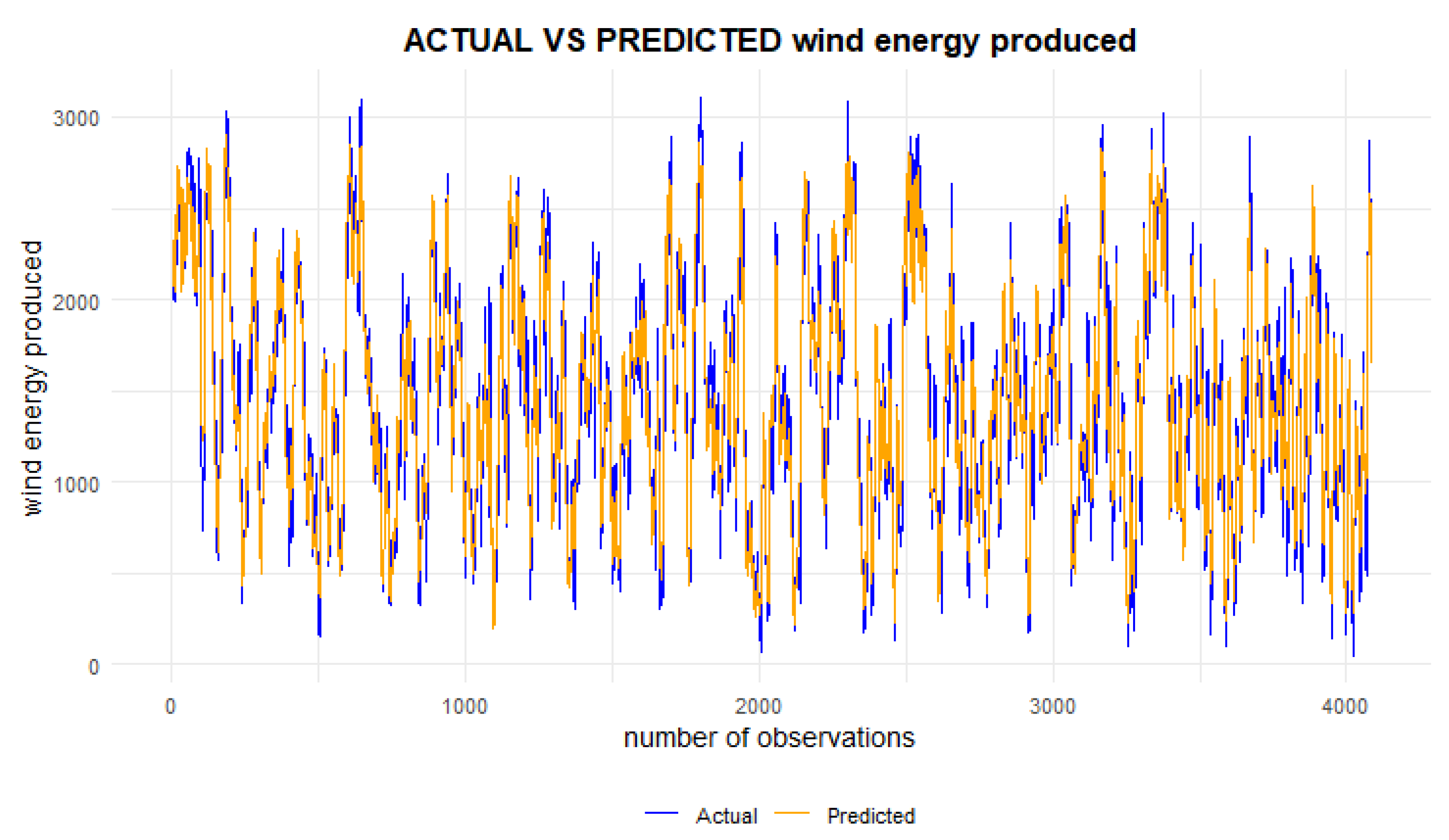
Figure 8.
Actual vs Predicted value at 80% training test, 10% validation and 10% test based on the sample of first 500 observations.
Figure 8.
Actual vs Predicted value at 80% training test, 10% validation and 10% test based on the sample of first 500 observations.
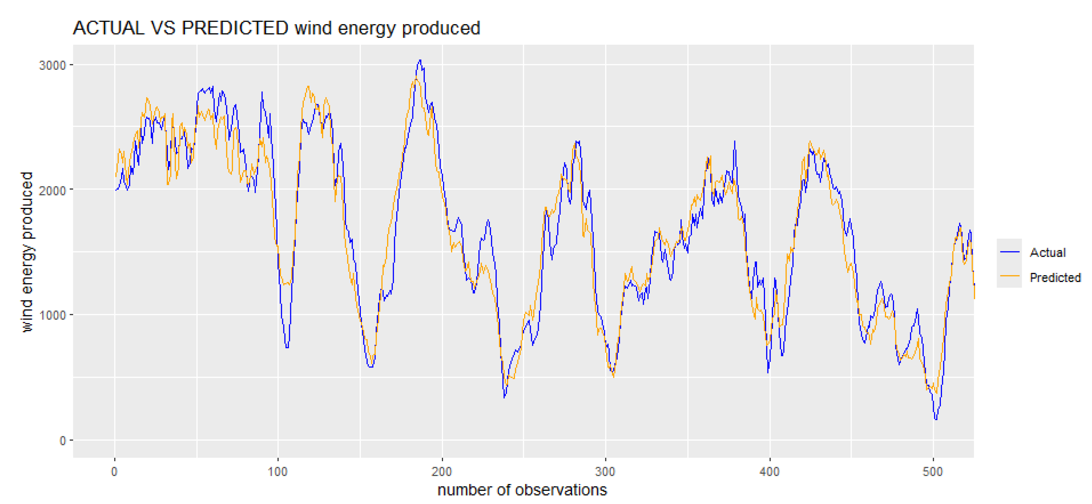
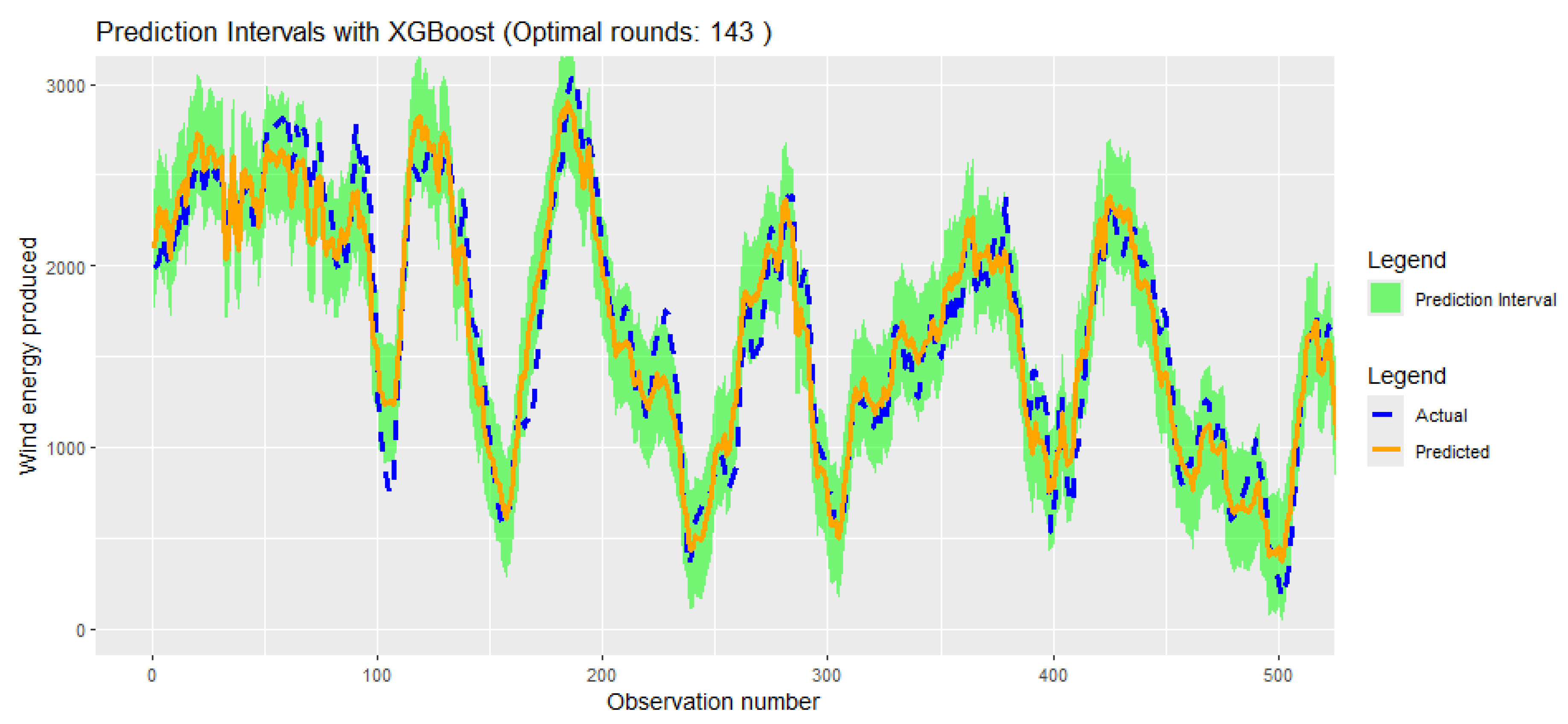
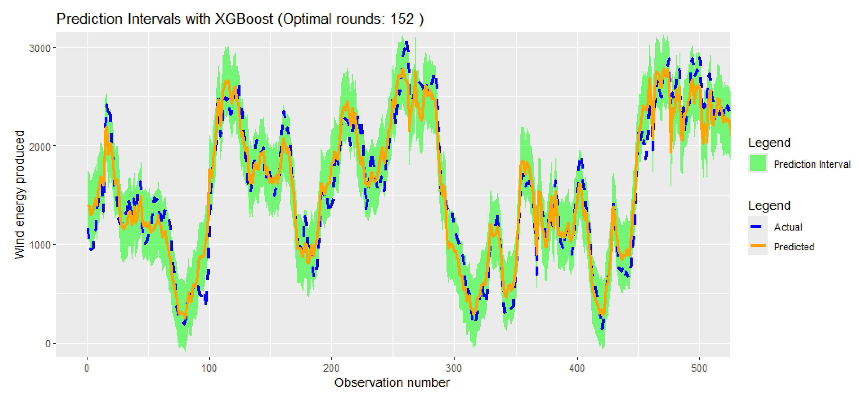
Figure 10, which is the zoomed sample of Figure 9 gives us that the XGBoost model shows strong and consistent performance in both point predictions and uncertainty quantification throughout the entire dataset. The Conformal Prediction Intervals effectively bound the actual wind energy produced across all segments, confirming that these intervals are well-calibrated and reliable.
Figure 9.
Conformal prediction interval at 80% training test, 10% validation and 10% test.
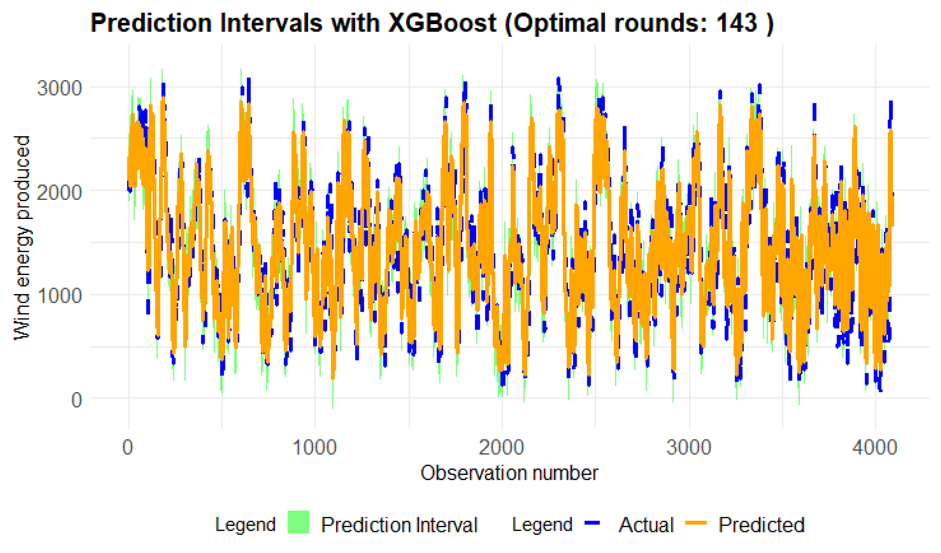
Figure 10.
Conformal Prediction iterval on Actual vs Predicted value at 80% training test, 10% validation and 10% test based on first 500 observations.
Figure 10.
Conformal Prediction iterval on Actual vs Predicted value at 80% training test, 10% validation and 10% test based on first 500 observations.
The series of plots clearly demonstrates that the predictive model, which was trained using an 80% training 10% validation and 10% test split, is highly effective in forecasting wind energy production. In the analysed figures, Figure 12, is the zoomed samples of Figure 11 which shows that the predicted values closely align with the actual production values.
Figure 11.
Conformal prediction interval at 85% training test, 10% validation and 5% test.
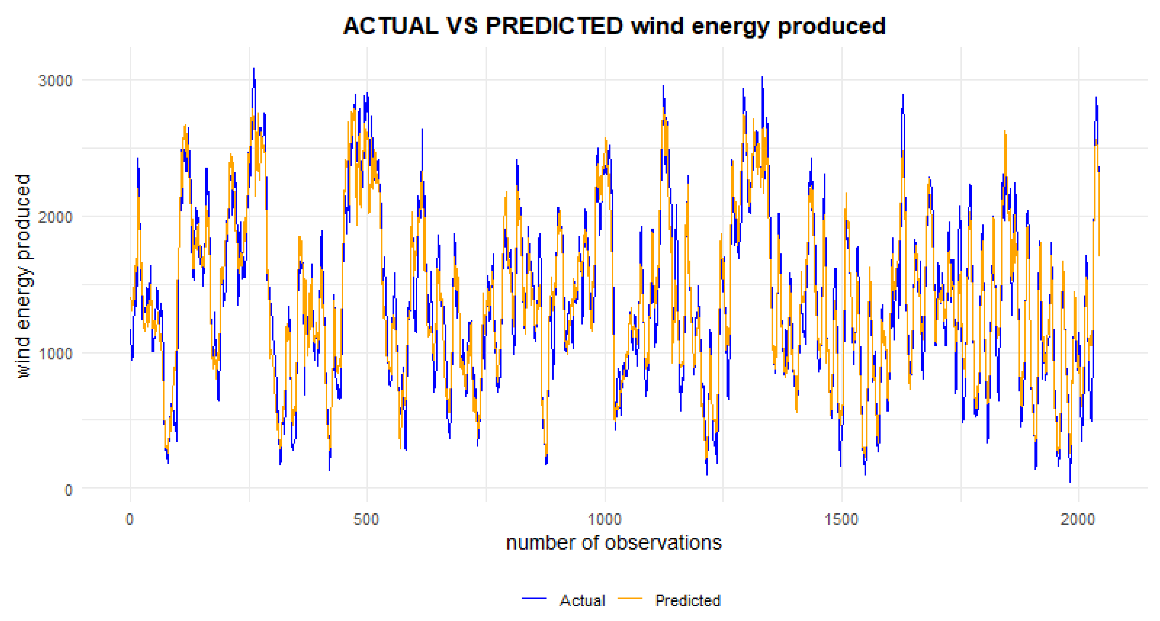
Figure 12.
Actual vs Predicted value at 80% training test, 10% validation and 5% test based on the first 500 observations.
Figure 12.
Actual vs Predicted value at 80% training test, 10% validation and 5% test based on the first 500 observations.
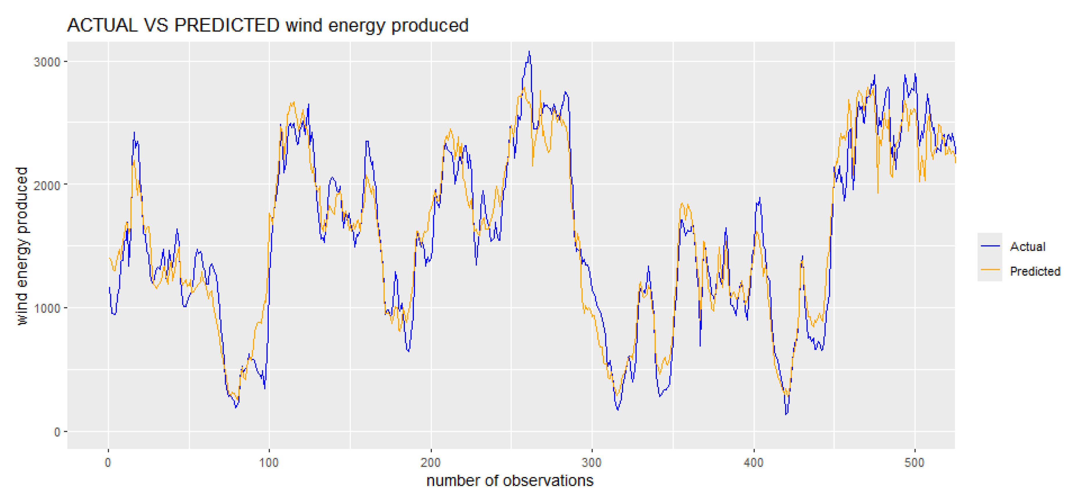
Figure 13.
Conformal prediction interval at 85% training test, 10 % validation and 5% test.
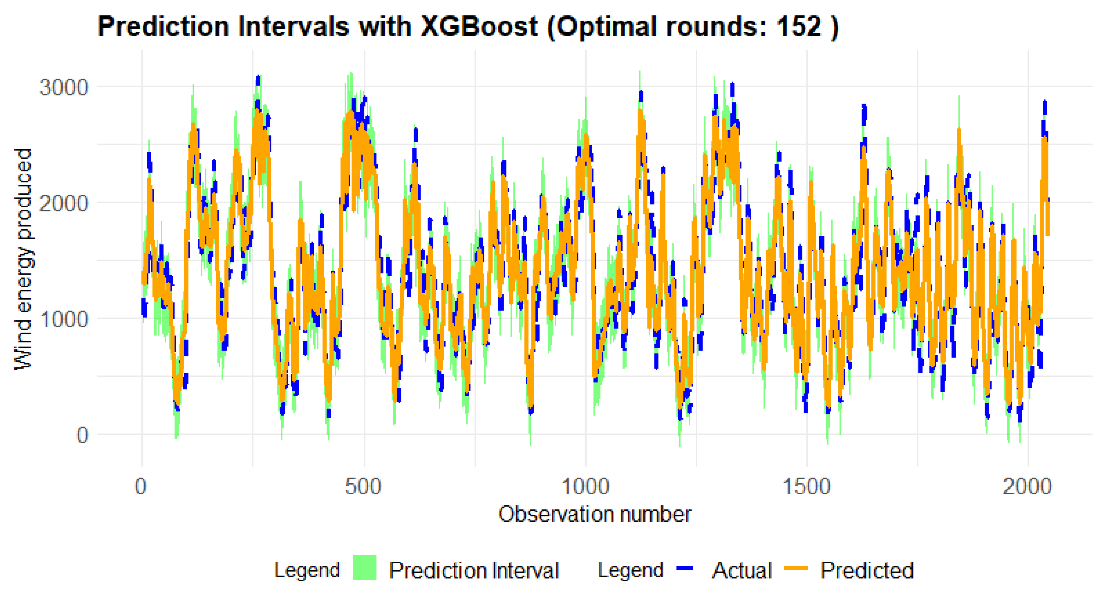
Figure 14.
Conformal Prediction interval of Actual vs Predicted value at 80% training test, 10% validation and 5% test.
Figure 14.
Conformal Prediction interval of Actual vs Predicted value at 80% training test, 10% validation and 5% test.
3.4. Principal Component Regression
3.5. Choosing Number of Components
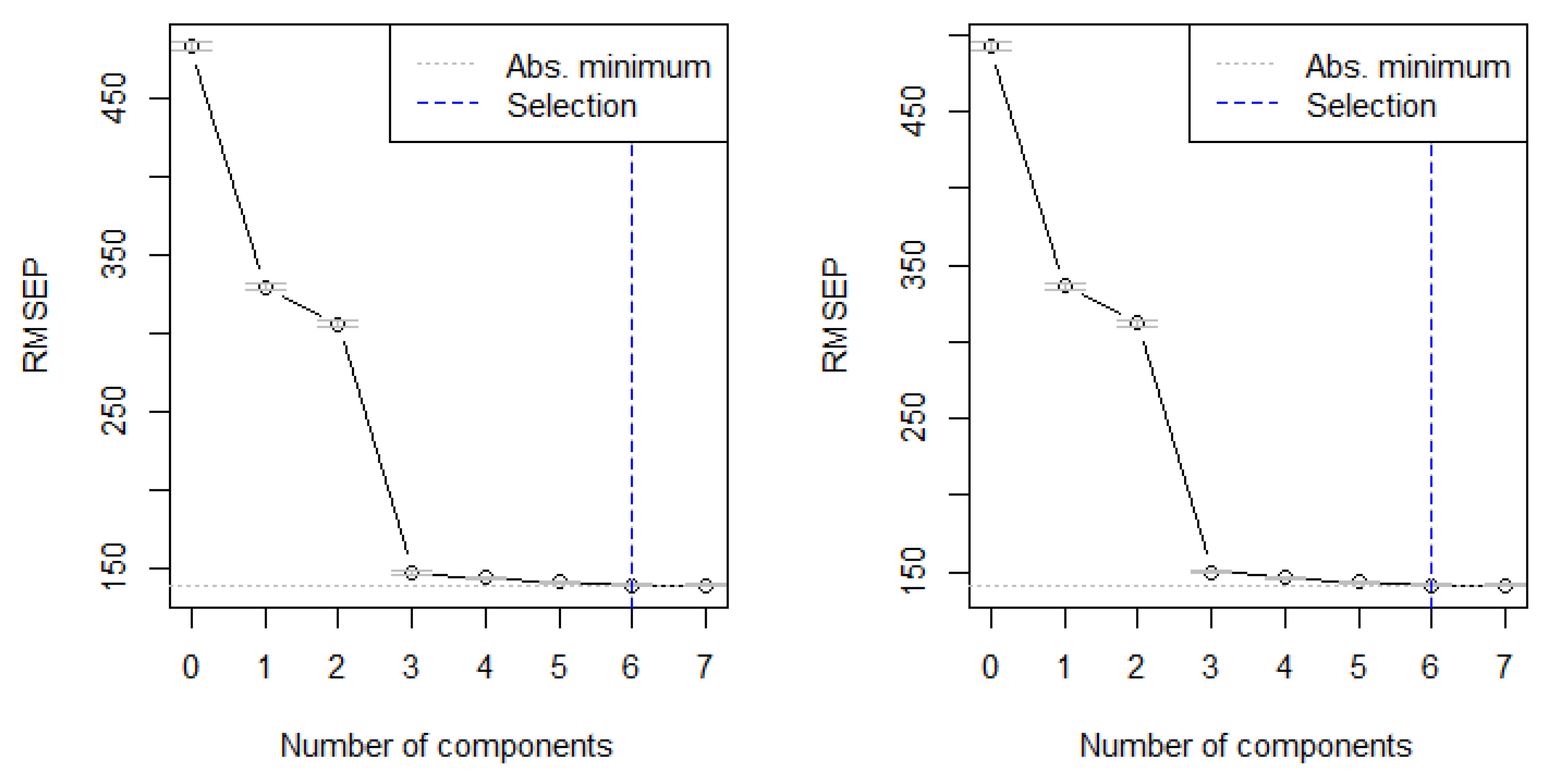
When selecting the optimal number of components for Principal Component Regression (PCR), the one-sigma heuristic was used. This approach is often recommended in the literature as a way to balance model simplicity and predictive accuracy. According to [15], the one-sigma heuristic involves choosing the model with the fewest components that still has a prediction error within one standard error of the minimum error observed across all models. In essence, rather than selecting the model with the absolute lowest prediction error, this method prioritises a simpler model that achieves nearly the same level of performance, thereby minimising the risk of overfitting.
3.6. Selecting Number of Components
Figure 15 illustrates the procedure for selecting the optimal number of components using the RMSEP criterion for both the 80% and 85% training sets. The plots show a sharp decline in RMSEP with the addition of the first few components, followed by a stabilization in RMSEP as more components are incorporated. While the absolute minimum RMSEP occurs at six components, the results indicate that most of the relevant predictive information is already captured by the first three to four components. Adding further components provides only marginal improvements to model performance.
Figure 15.
Selecting number of optimal components for 80% and 85% training test.
3.7. Actual vs Predicted
Figure 16.
Actual vs predicted value of 10% test set on benchmark model.
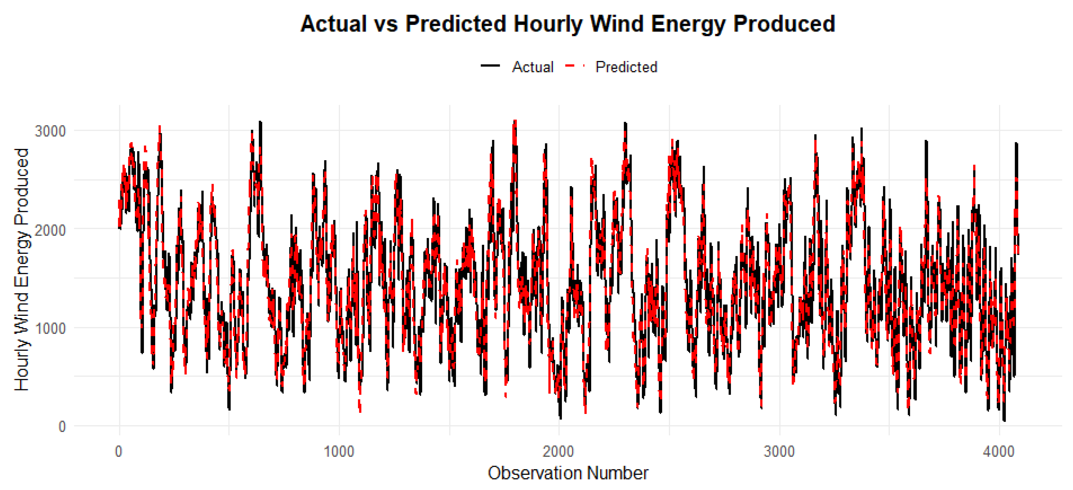
Figure 17.
Actual vs predicted value of 5% test set on benchmark model.
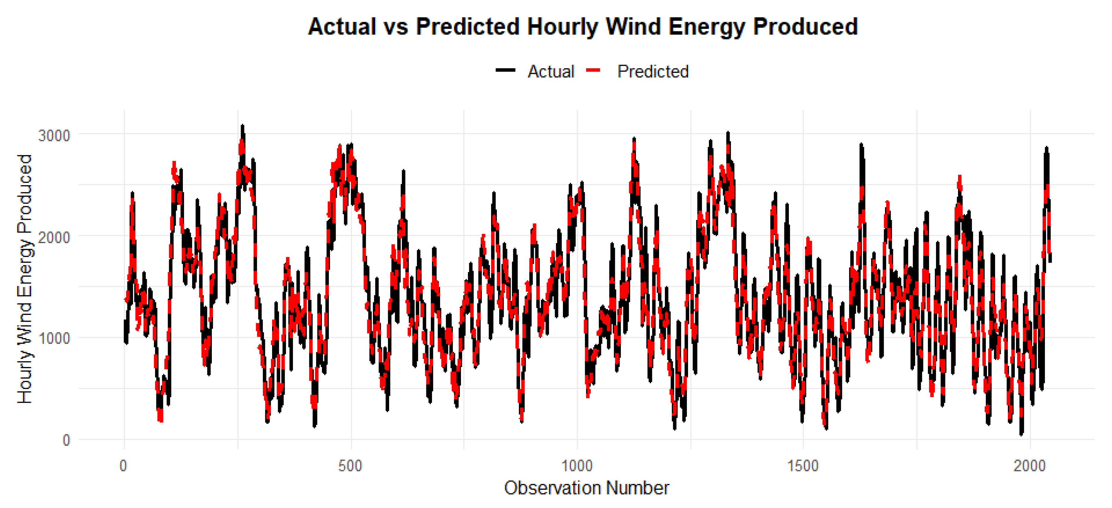

Table 4.
Model performance comparison using (80% training test, 10% validation and 10% test) and (85% training test, 10% validation and 5% test).
Table 4.
Model performance comparison using (80% training test, 10% validation and 10% test) and (85% training test, 10% validation and 5% test).
| Model/Set | Evaluation Metrics | Values |
|---|---|---|
| 80% train | MASE | 1.382165 |
| 10% validation | RMSE | 189.0324 |
| 10% test | MAE | 149.9833 |
| MBE | -3.465533 | |
| Model/Set | Evaluation Metrics | Values |
| 85% train | MASE | 1.322423 |
| 10% validation | RMSE | 190.2073 |
| 5% test | MAE | 144.6136 |
| MBE | -4.108761 |
Table 5.
Evaluation metrics for the prediction intervals on (80% training test, 10% validation and 10% test) and (85% training test, 10% validation and 5% test).
Table 5.
Evaluation metrics for the prediction intervals on (80% training test, 10% validation and 10% test) and (85% training test, 10% validation and 5% test).
| Model/Set | Evaluation Metrics | Values |
|---|---|---|
| 80% train | PICP | 0.927522 |
| 10% validation | MPIW | 654.7578 |
| 10% test | CWC | 2669.333 |
| Model/Set | Evaluation Metrics | Values |
| 85% train | PICP | 0.9363681 |
| 10% validation | MPIW | 693.342 |
| 5% test | CWC | 2064.1 |
Figure 18 and Figure 19 present Probability Integral Transform (PIT) histograms, which is derived from conformal p-values, which serve as a standard diagnostic tool for assessing the probabilistic calibration of a forecasting model. Both histograms provide strong visual evidence that the conformal prediction model is well-calibrated. In both plots, the distribution of the p-values is approximately uniform, which is the desired outcome. This consistency across both graphs confirms that the model’s estimates of uncertainty are reliable.
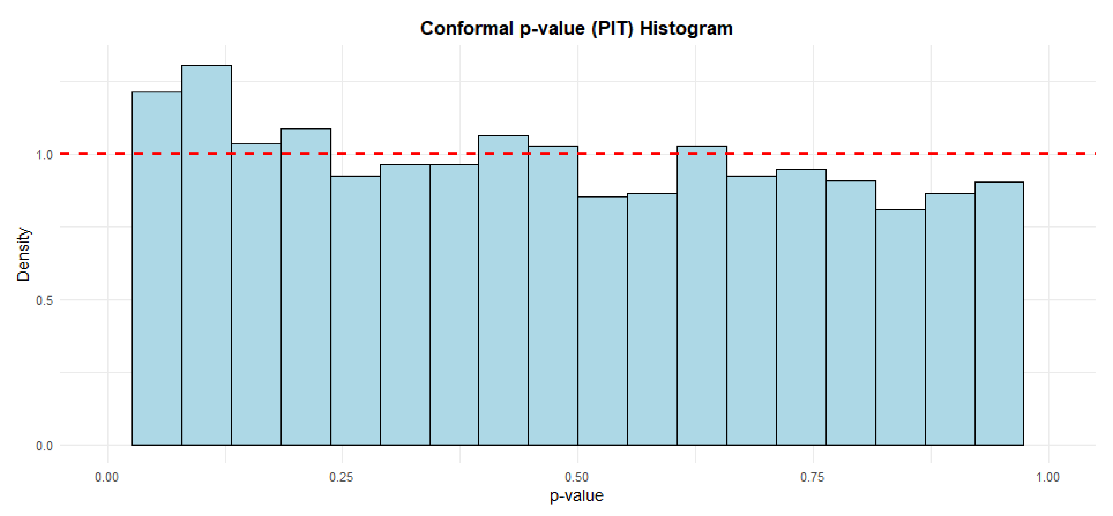
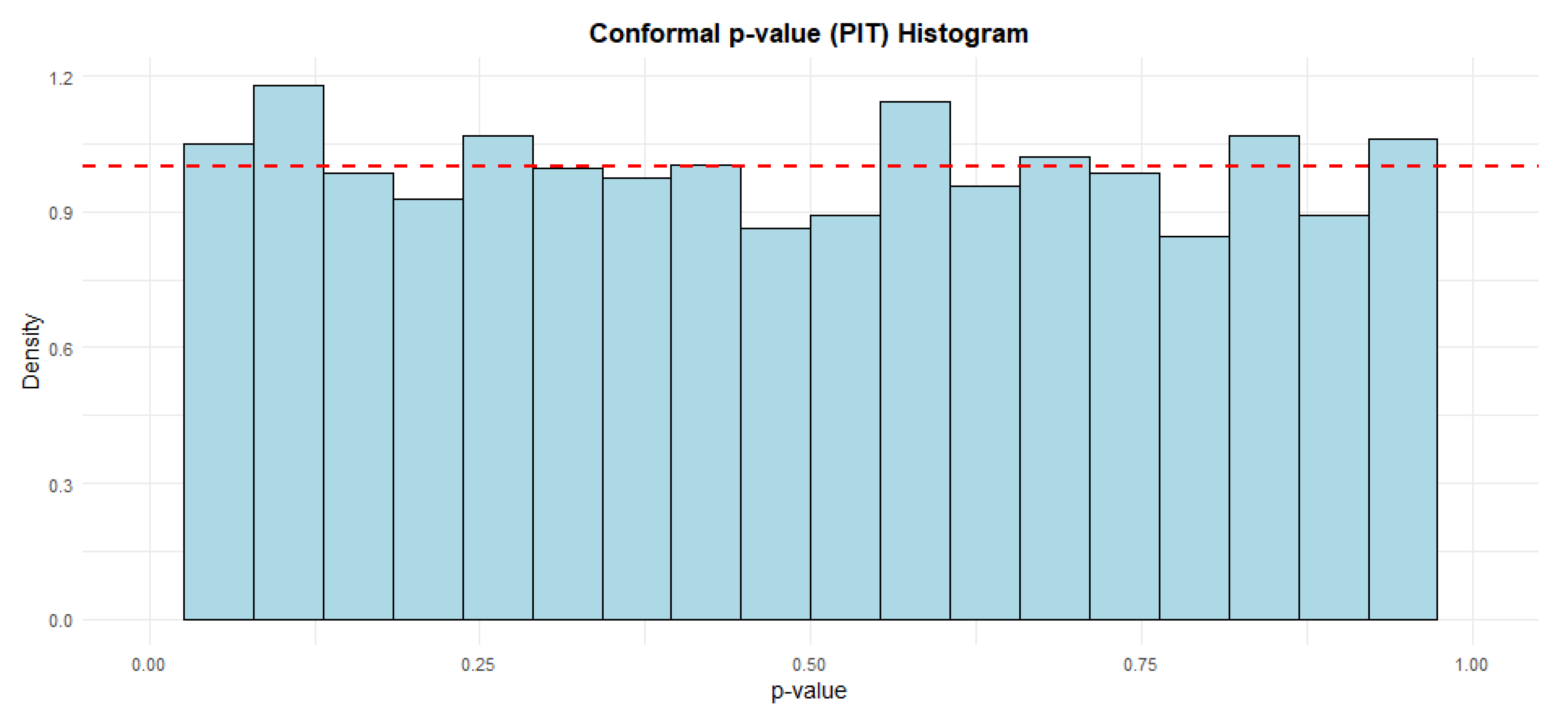
Figure 18.
Probability Integral Transform on (80% training test, 10% validation and 10% test).
Figure 19.
Probability Integral Transform on (85% training test, 10% validation and 5% test).
3.8. Probability of Change in Direction and Fitness Tests
3.8.1. XGBoost and PCR (80% Training Test, 10% Validation and 10% Test)
Based on the 80% training test, 10% validation and 10% test sets for both the XGBoost and PCR models we combined predictions of the test set using the partially linear additive quantile regression (PLAQR) averaging method. We refer to the combined predictions as . A detailed discussion of the PLAQR method is discussed in [29].
The evaluation compared three forecasting models, , and , using a combination of traditional error metrics, directional accuracy, and a composite fitness score. A summary of the model comparison (80% training test, 10% validation and 10% test) is given in Table 6, while Figure 20 shows the probability of change in direction. In terms of directional accuracy, measured by the Prediction of Change in Direction (POCID), all models performed well, with scores ranging from 70.71% to 71.71%. Model achieved the highest directional accuracy at 71.71%. However, when considering prediction error, recorded the lowest Root Mean Squared Error (RMSE) of approximately 179, while had the highest RMSE at about 189.
To provide an overall assessment, a fitness metric was used that balances directional accuracy with error magnitude, applying a weight factor optimised for the observed RMSE range. According to this combined measure, model achieved the highest fitness score of 34.28, making it the best-performing model overall. This outcome reflects its superior balance between maintaining a relatively high POCID and keeping prediction errors low. Models and followed with fitness scores of 33.76 and 33.60, respectively.
Figure 20.
Probability of change in direction (80% training test, 10% validation and 10% test).
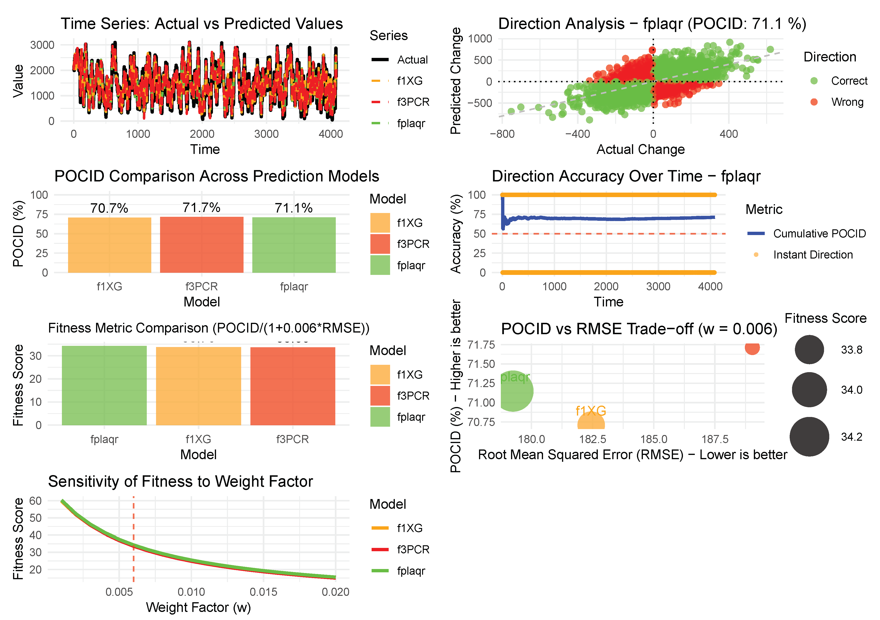
While each model demonstrated solid performance, is identified as the most effective, offering the optimal trade-off between accurately predicting movement direction and minimising forecast error. The fitness metric, calibrated with a weight of 0.006, effectively highlighted these differences, confirming as the recommended choice for practical application.
3.8.2. XGBoost and PCR (85% Training Test, 10% Validation and 5% Test)
Similarly for the 85% training test, 10% validation and 5% test sets the combined predictions using PLAQR is referred to as . The results given in Table 7 compare three models: , and , using error metrics, directional accuracy, and a combined fitness score, while Figure 21 shows the probability of change in direction. In traditional error measures, fplaqr performs best, with the lowest MAE (139.12), MSE (32,000.81), RMSE (178.89), and MASE (1.22), indicating the smallest average prediction errors. The models and follow with progressively higher error values. All models show a low mean bias error (MBE), suggesting minimal systematic over- or under-prediction.
For directional accuracy, measured by POCID, fplaqr again leads by correctly predicting price movement direction 74.24% of the time, compared to 72.97% for f2XG and 73.31% for . A combined fitness metric, which balances POCID against RMSE with a weighting factor of 0.006, ranks the models in the same order: . achieves the highest fitness score (35.81), followed by and . All are interpreted as having “good" overall performance.
Figure 21.
Probability of change in direction (85% training test, 10% validation and 5% test).
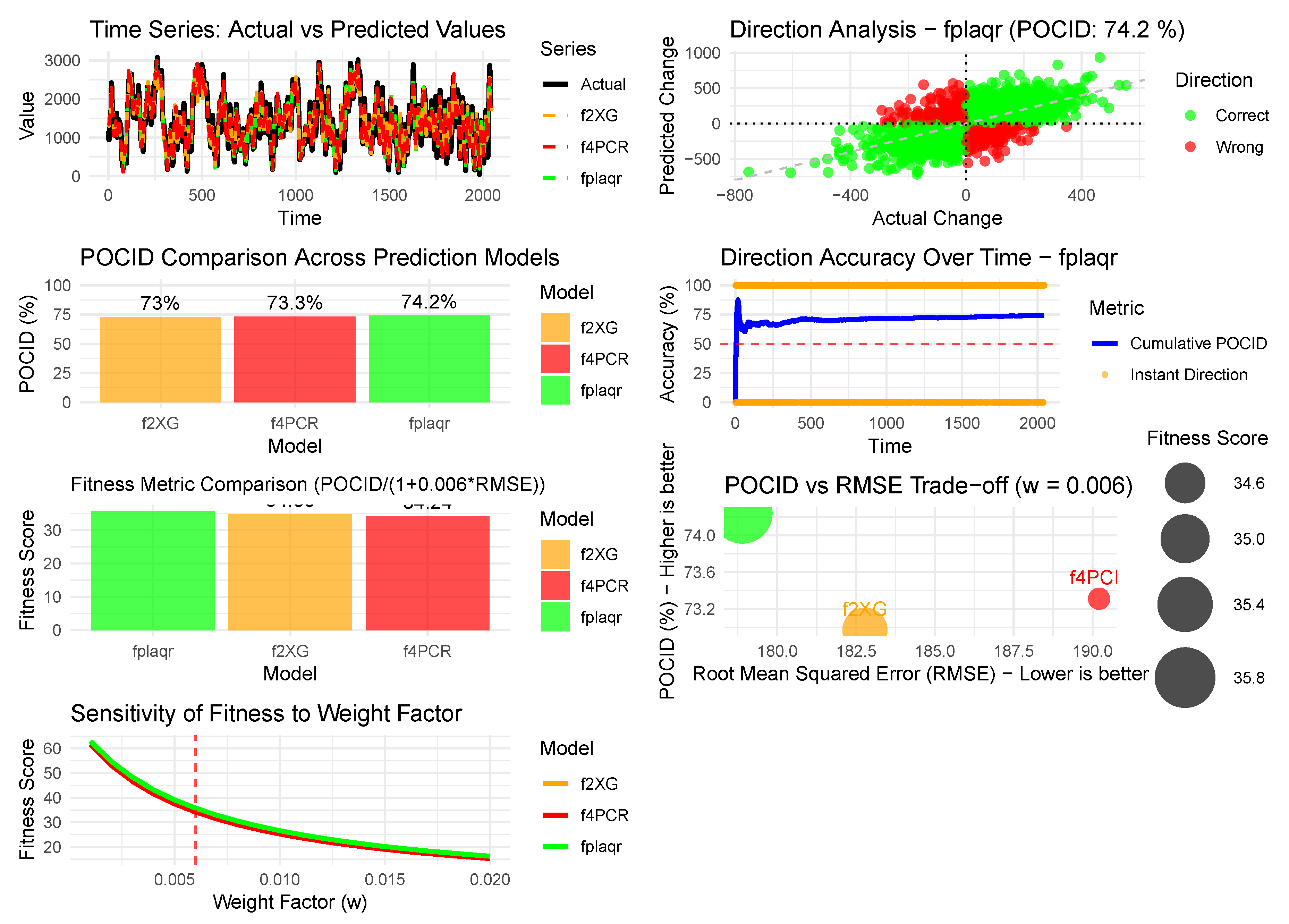
The analysis confirms that . is the best-performing model across both accuracy and directional metrics. The chosen weight () is justified as approximately the inverse of the average RMSE across models, providing an optimal penalty that allows for meaningful comparison without overly diminishing the fitness score. The results suggest this weighting is appropriate for models with RMSE values around 180-190.
4. Discussion
This research shows that the hybrid model produced by combining XGBoost and PCR via the PLAQR averaging method is better calibrated and more accurate. This result, that the PLAQR ensemble model is better for composite performance (), is consistent with the established notion within the research community that model averaging is preferable, as it helps reduce variance and become more generalizable [30,31]. However, this has been made possible within the conformal prediction paradigm, as indicated through its well-calibrated predictions as well as its PIT Histograms, which is a major development as it proves that advanced combination methods are capable of improving both accuracy as well as probability values within machine learning paradigms despite primarily focusing on error minimisation within their model development approaches.
The superior directional accuracy (POCID) and reduced error (RMSE) of the PLAQR model confirm our hypothesis: it can indeed capture complex nonlinearities by leveraging the complementary strengths of tree-based and linear methods, while maintaining structural stability. The competitive POCID of the PCR model, along with its higher error, flags its sensitivity to directional trends but with limitations in magnitude precision.XGBoost, on the other hand, provided a compromise solution. More importantly, the performance gain with the larger training dataset (85% vs. 80%) indicates that these data-intensive models continue to benefit from more data, underscoring the significance of scale in wind energy forecasting models.
The implications of these findings extend beyond this specific forecasting problem. They provide one possible solution to the problem of constructing reliable forecasting systems in the renewable energy sector. The success of the conformal prediction method is important for understanding how to construct more trustworthy AI systems in problem domains where reliable estimates of uncertainty are important.
The effectiveness of the PLAQR approach needs to be tested with a more diverse ensemble, including other model types, such as neural networks and scoring functions. The robustness of this approach can also be tested using high-frequency time-series data. Another area could be exploring adaptive weights for the PLAQR model.
5. Conclusion
This study shows that the PLAQR ensemble of XGBoost and PCR provides a well-calibrated, superior forecasting model, both in terms of accuracy (RMSE, POCID) and probabilistic reliability, as measured by conformal prediction. The current study thereby reassures that advanced averaging techniques can benefit both point forecasts and uncertainty quantification in machine learning. The results demonstrate the importance of combining model classes and using larger data sets for renewable energy forecasting.
Author Contributions
Conceptualization, R.I.N., T.H.T., T.R. and C.S.; methodology, R.I.N.; software, R.I.N.; validation, R.I.N., T.H.T., T.R. and C.S.; formal analysis, R.I.N., C.S.; investigation, R.I.N., T.H.T., T.R. and C.S.; data curation, R.I.N.,; writing—original draft preparation, R.I.N.; writing—review and editing, R.I.N., T.H.T., T.R. and C.S.; visualization, R.I.N.; supervision, T.H.T., T.R. and C.S.; project administration, T.H.T., T.R. and C.S. All authors have read and agreed to the published version of the manuscript.
Funding
This research received no external funding and the APC was funded by the university of Venda.
Data Availability Statement
The data that support the findings of this study are available at https://github.com/csigauke/Enhancing-Short-Term-Wind-Energy-Forecasting-with-XGBoost-and-Conformal-Prediction. The data is analytic data which was used for developing the models used in this study.
Acknowledgments
The authors are grateful to the numerous people for helpful comments on this paper.
Conflicts of Interest
The authors declare no conflicts of interest.
Abbreviations
The following abbreviations are used in this manuscript:
| ANN | Artificial Neural Networks |
| ARIMA | AutoRegressive Integrated Moving Average |
| BH-XGBoost | Bayesian Hyperparameter-optimised XGBoost |
| Boost-LR | Boosting with Linear Regression |
| CNN GRU | Convolutional Neural Network and Gated Recurrent Unit |
| CWC | Coverage Width-based Criterion |
| GBM | Gradient Boosting Machines |
| GPR | Gaussian Process Regression |
| KDJ | Stochastic Oscillator |
| KNN | K-Nearest Neighbors |
| LSTM | Long Short-Term Memory |
| MACD | Moving Average Convergence and Divergence |
| MAE | Mean Absolute Error |
| MASE | Mean Absolute Scaled Error |
| MBE | Mean Bias Error |
| MLP ANN | Multi-Layer Perceptron Artificial Neural Network |
| MPIW | Mean Prediction Interval Width |
| NMAE | Normalised Mean Absolute Error |
| NN | Neural Networks |
| PCA | Principal Component Analysis |
| PCR | Principal Component Regression |
| PICP | Prediction Interval Coverage Probability |
| PIT | Probability Integral Transform |
| RF | Random Forest |
| RMSE | Root Mean Square Error |
| SVM | Support Vector Machines |
| XGBoost | eXtreme Gradient Boosting |
References
- Behabtu, H.A.; Vafaeipour, M.; Kebede, A.A.; Berecibar, M.; Van Mierlo, J.; Fante, K.A.; Messagie, M.; Coosemans, T. Smoothing Intermittent Output Power in Grid-Connected Doubly Fed Induction Generator Wind Turbines with Li-Ion Batteries. Energies 2023, 16. [Google Scholar] [CrossRef]
- Kim, D.; Hur, J. Short-term probabilistic forecasting of wind energy resources using the enhanced ensemble method. Energy 2018, 157, 211–226. [Google Scholar] [CrossRef]
- Foley, A.M.; Leahy, P.G.; Marvuglia, A.; McKeogh, E.J. Current methods and advances in forecasting of wind power generation. Renewable Energy 2012, 37, 1–8. [Google Scholar] [CrossRef]
- Zheng, Y.; Guan, S.; Guo, K.; Zhao, Y.; Ye, L. Technical indicator enhanced ultra-short-term wind power forecasting based on long short-term memory network combined XGBoost algorithm. IET Renewable Power Generation 2025, 19, e12952. [Google Scholar] [CrossRef]
- Ekinci, G.; Ozturk, H.K. Forecasting Wind Farm Production in the Short, Medium, and Long Terms Using Various Machine Learning Algorithms. Energies 2025, 18, 1125. [Google Scholar] [CrossRef]
- Giebel, G.; Brownsword, R.; Kariniotakis, G.; Denhard, M.; Draxl, C. The state-of-the-art in short-term prediction of wind power: A literature overview. Project Report: ANEMOS.plus 2011.
- Lei, M.; Shiyan, L.; Chuanwen, J.; Hongling, L.; Yan, Z. A review on the forecasting of wind speed and generated power. Renewable and Sustainable Energy Reviews 2009, 13, 915–920. [Google Scholar] [CrossRef]
- Park, S.; Jung, S.; Lee, J.; Hur, J. A short-term forecasting of wind power outputs based on gradient boosting regression tree algorithms. Energies 2023, 16, 1132. [Google Scholar] [CrossRef]
- Chen, T.; Guestrin, C. XGBoost: A Scalable Tree Boosting System. In Proceedings of the 22nd ACM SIGKDD International Conference on Knowledge Discovery and Data Mining, 2016; pp. 785–794. [Google Scholar]
- Xiong, X.; Guo, X.; Zeng, P.; Zou, R.; Wang, X. A short-term wind power forecast method via XGBoost hyper-parameters optimization. Frontiers in Energy Research 2022, 10, 905155. [Google Scholar] [CrossRef]
- García-Puente, B.; Rodríguez-Hurtado, A.; Santos, M.; Sierra-García, J. Evaluation of XGBoost vs. other Machine Learning models for wind parameters identification. Renewable Energy and Power Quality Journal 2023, 21, 388–393. [Google Scholar] [CrossRef]
- Lahouar, A.; Slama, J.B.H. Hour-ahead wind power forecast based on random forests. Renewable Energy 2017, 109, 529–541. [Google Scholar] [CrossRef]
- Sunku, V.S.R.P.; Namboodiri, V.; Mukkamala, R. The Short-Term Wind Power Forecasting by Utilizing Machine Learning and Hybrid Deep Learning Frameworks. Problems of the Regional Energetics; 2025. [Google Scholar]
- Ahmed, U.; Muhammad, R.; Abbas, S.S.; Aziz, I.; Mahmood, A. Short-term wind power forecasting using integrated boosting approach. Frontiers in Energy Research 2024, 12, 1401978. [Google Scholar] [CrossRef]
- Mevik, B.H.; Wehrens, R. Introduction to the pls Package. R Package Documentation 2015, 1–23. [Google Scholar]
- Kavzoglu, T.; Teke, A. Advanced hyperparameter optimization for improved spatial prediction of shallow landslides using extreme gradient boosting (XGBoost). Bulletin of Engineering Geology and the Environment 2022, 81, 201. [Google Scholar] [CrossRef]
- Liu, Z.; Guo, H.; Zhang, Y.; Zuo, Z. A Comprehensive Review of Wind Power Prediction Based on Machine Learning: Models, Applications, and Challenges. Energies 2025, 18, 350. [Google Scholar] [CrossRef]
- Ponkumar, G.; Jayaprakash, S.; Kanagarathinam, K. Advanced machine learning techniques for accurate very-short-term wind power forecasting in wind energy systems using historical data analysis. Energies 2023, 16, 5459. [Google Scholar] [CrossRef]
- Vovk, V.; Gammerman, A.; Shafer, G. Algorithmic learning in a random world; Springer, 2005. [Google Scholar]
- Angelopoulos, A.N.; Bates, S. A gentle introduction to conformal prediction and distribution-free uncertainty quantification. arXiv 2021, arXiv:2107.07511. [Google Scholar]
- Dheur, V. Distribution-Free and Calibrated Predictive Uncertainty in Probabilistic Machine Learning. PhD thesis, UMONS - University of Mons [Faculté des Sciences], Mons, Belgium, 2025. Available online: https://orbi.umons.ac.be/20.500.12907/54123.
- Zhao, X.; Li, Q.; Xue, W.; Zhao, Y.; Zhao, H.; Guo, S. Research on Ultra-Short-Term Load Forecasting Based on Real-Time Electricity Price and Window-Based XGBoost Model. Energies 2022, 15. [Google Scholar] [CrossRef]
- Friedman, J.H. Stochastic gradient boosting. Computational Statistics and Data Analysis 2002, 38, 367–378. [Google Scholar] [CrossRef]
- Chen, T.; He, T.; Benesty, M.; Khotilovich, V.; Tang, Y.; Cho, H.; Chen, K.; Mitchell, R.; Cano, I.; Zhou, T.; et al. R package version 0.4-22015; Xgboost: extreme gradient boosting. 1, pp. 1–4. [CrossRef]
- Fallahtafti, A.; Aghaaminiha, M.; Akbarghanadian, S.; et al. Forecasting ATM Cash Demand Before and During the COVID-19 Pandemic Using an Extensive Evaluation of Statistical and Machine Learning Models. SN Computer Science 2022, 3. [Google Scholar] [CrossRef]
- Stocker, M.; Małgorzewicz, W.; Fontana, M.; Taieb, S.B. A Gentle Introduction to Conformal Time Series Forecasting. arXiv 2025, arXiv:2511.13608. [Google Scholar] [CrossRef]
- Khosravi, A.; Nahavandi, S.; Creighton, D.; Atiya, A.F. Comprehensive review of neural network-based prediction intervals and new advances. IEEE Transactions on Neural Networks 2011, 22, 1341–1356. [Google Scholar] [CrossRef]
- Gneiting, T.; Balabdaoui, F.; Raftery, A.E. Probabilistic forecasts, calibration and sharpness. Journal of the Royal Statistical Society Series B: Statistical Methodology 2007, 69, 243–268. [Google Scholar] [CrossRef]
- Hoshino, T. Quantile regression estimation of partially linear additive models. Journal of Nonparametric Statistics 2014, 26, 509–536. [Google Scholar] [CrossRef]
- Nowotarski, J.; Weron, R. Computing electricity spot price prediction intervals using quantile regression and forecast averaging. Computational Statistics 2015, 30, 791–803. [Google Scholar] [CrossRef]
- Mpfumali, P.; Sigauke, C.; Bere, A.; Mulaudzi, S. Day Ahead Hourly Global Horizontal Irradiance Forecasting—Application to South African Data. Energies 2019, 12, 3569. [Google Scholar] [CrossRef]
Figure 1.
Flowchart of the modelling framework.
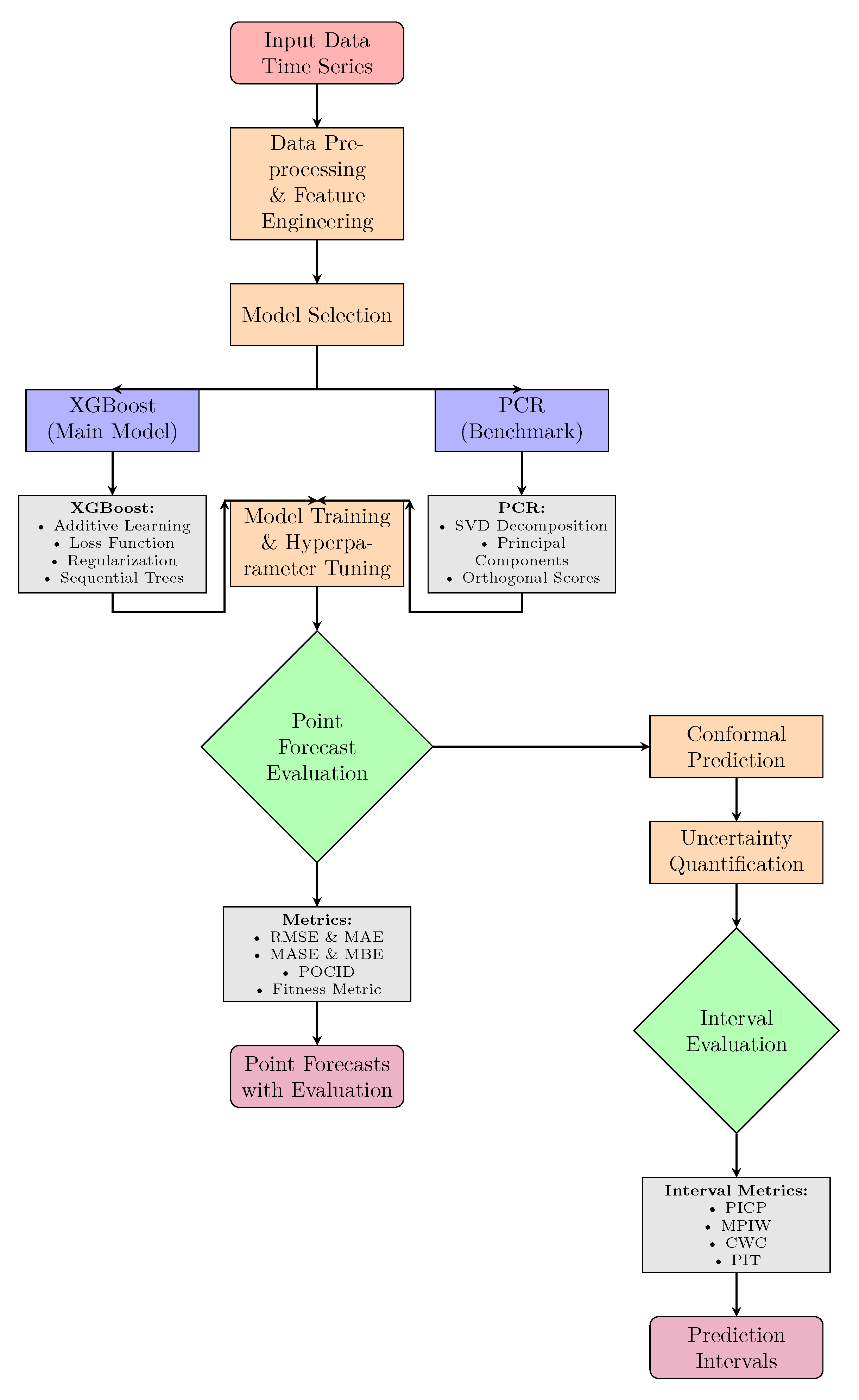
Figure 2.
Distribution of variables.
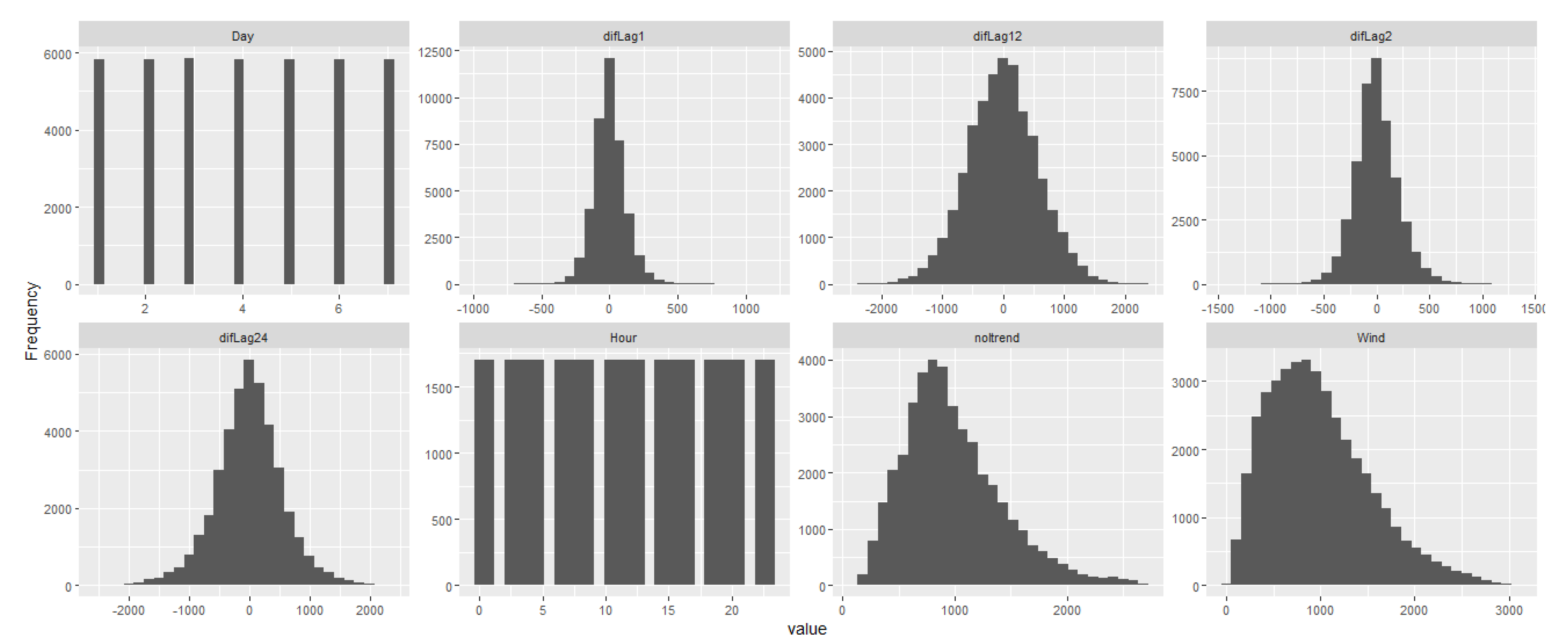
Figure 3.
time series wind plot.
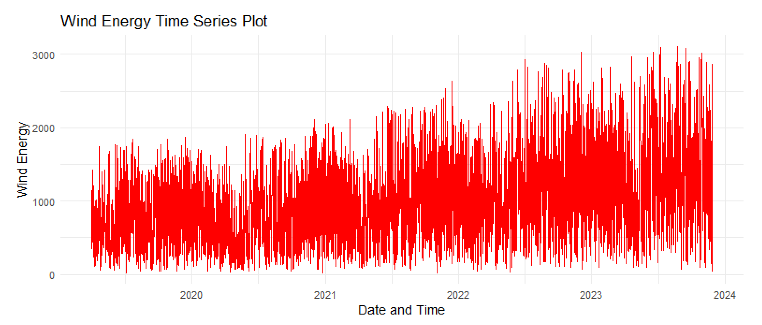
Figure 4.
Missing value.
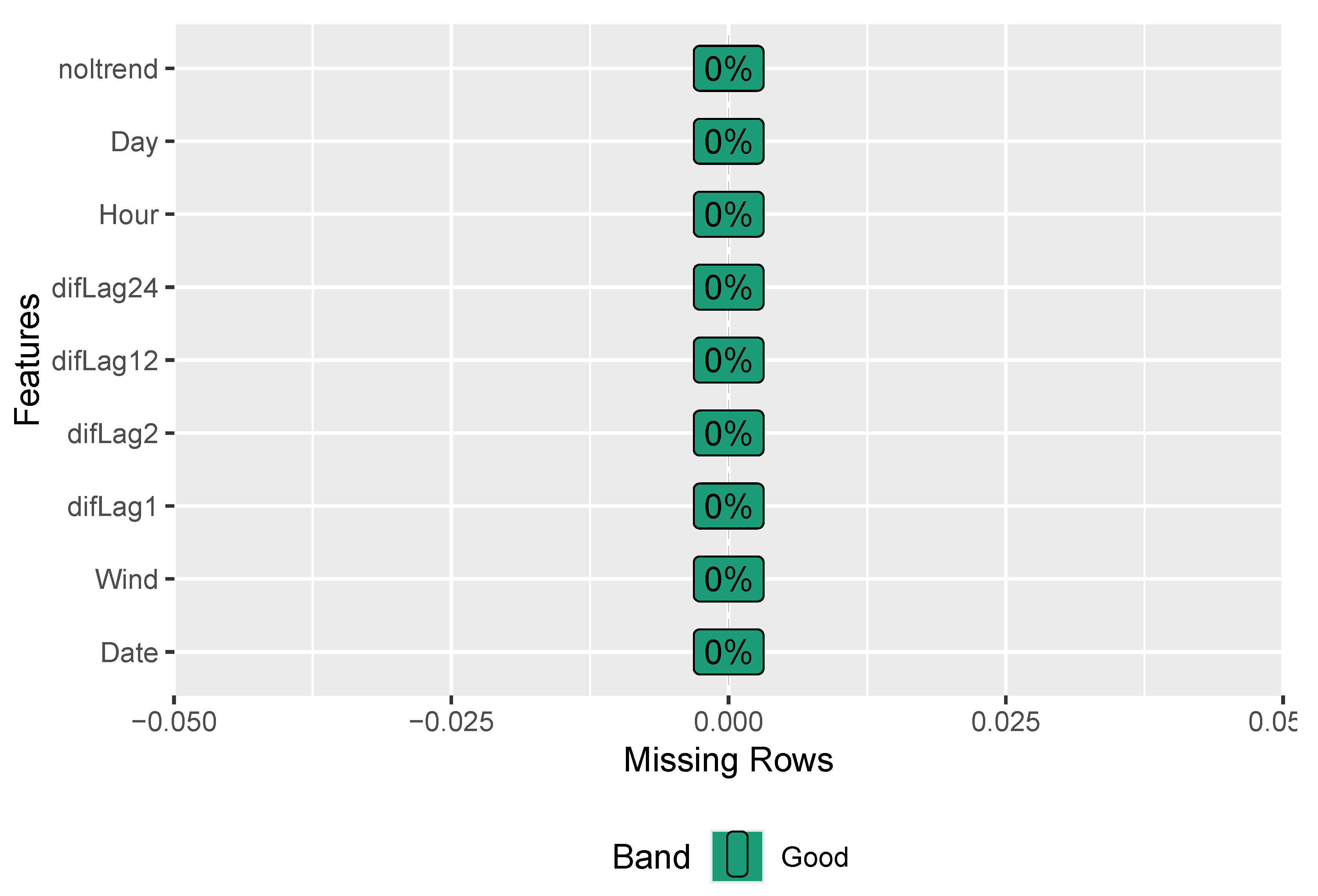
Figure 5.
Pearson correlation coefficient matrix.
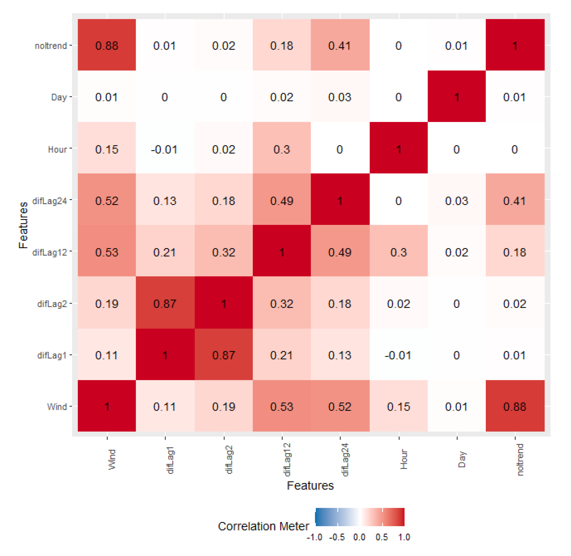
Figure 6.
Variable importance for 80% train set and 85% train set.
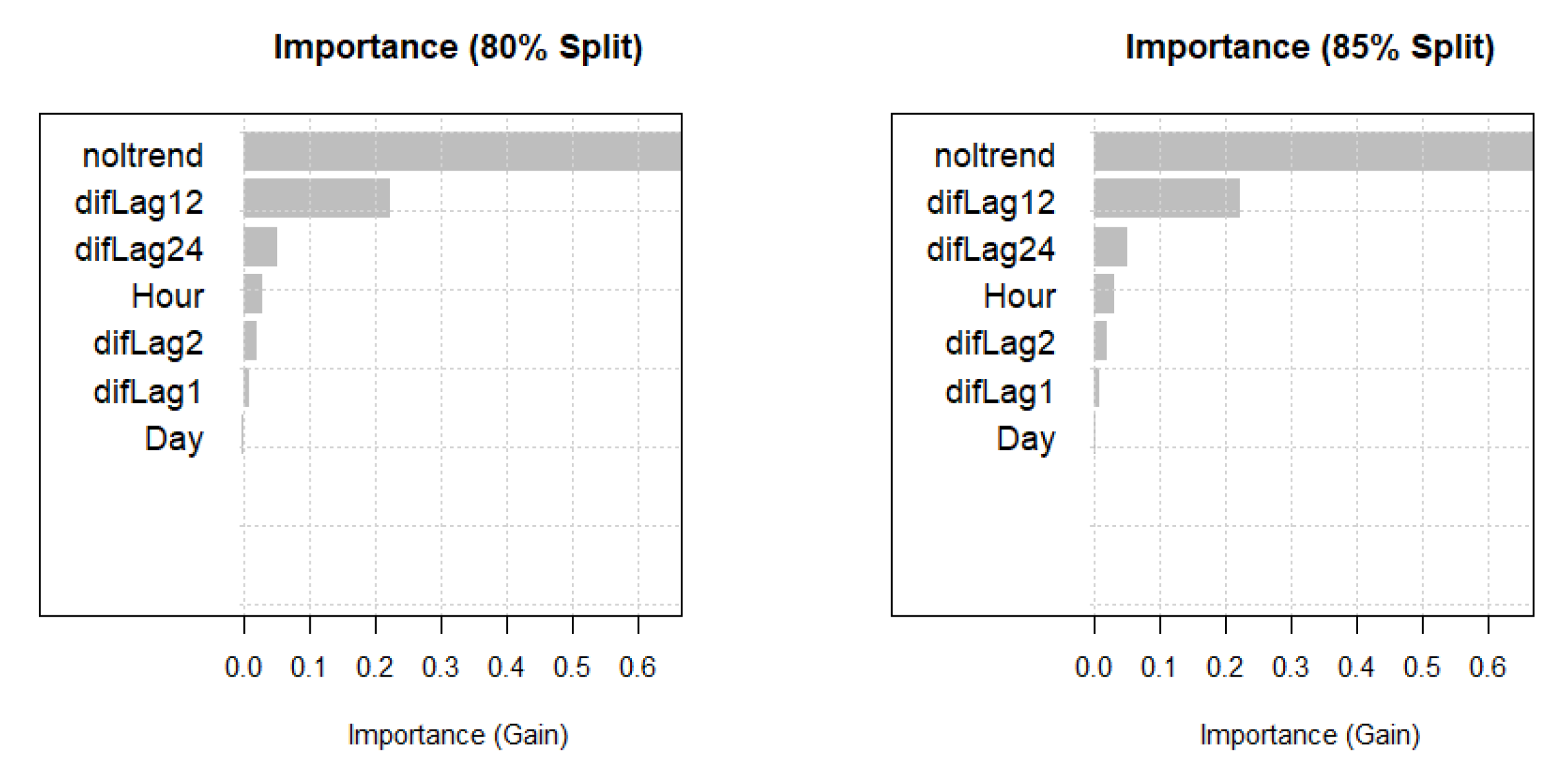
Table 1.
Summary statistics for wind energy produced.
| Summary | Value |
|---|---|
| Minimum | 19.8 |
| First Quartile (Q1) | 568.4 |
| Median (Q2) | 903.0 |
| Third Quartile (Q3) | 1306.8 |
| Maximum | 3102.2 |
| Mean | 982.5 |
| Skewness | 0.7557056 |
| Kurtosis | 3.305725 |
Table 2.
Variable importance comparison for 80% and 85% training sets.
| Variables | Importance (80% Train) | Importance (85% Train) |
|---|---|---|
| noltrend | 0.663583187 | 0.666984933 |
| difLag12 | 0.230901594 | 0.222293740 |
| difLag24 | 0.060511604 | 0.050816193 |
| Hour | 0.019899308 | 0.030228363 |
| difLag2 | 0.016097207 | 0.019848611 |
| difLag1 | 0.007545666 | 0.008239387 |
| Day | 0.001461434 | 0.001588773 |
Table 3.
Model performance comparison using (80% training test, 10% validation and 10% test) and (85% training test, 10% validation and 5% test).
Table 3.
Model performance comparison using (80% training test, 10% validation and 10% test) and (85% training test, 10% validation and 5% test).
| Model/Set | Evaluation Metrics | Optimal Rounds=143 | nrounds=500 | nrounds=1000 |
|---|---|---|---|---|
| 80% train | MASE | 1.328386 | 1.403668 | 1.418826 |
| 10% validation | RMSE | 182.4441 | 193.5536 | 195.9357 |
| 10% test | MAE | 144.1475 | 152.3166 | 153.9614 |
| MBE | 0.06772227 | -7.108178 | -7.973256 | |
| Model/Set | Evaluation Metrics | Optimal Rounds=152 | nrounds=500 | nrounds=1000 |
| 85% train | MASE | 1.255125 | 1.314607 | 1.342063 |
| 10% validation | RMSE | 182.781 | 192.4822 | 197.4568 |
| 5% test | MAE | 143.5088 | 150.3099 | 153.4492 |
| MBE | -3.731113 | -17.54136 | -12.73862 |
Table 6.
Comprehensive Model Comparison (80% training test, 10% validation and 10% test)
| Model | MASE | RMSE | MSE | MAE | MBE | POCID (%) | Fitness |
|---|---|---|---|---|---|---|---|
| 1.2993 | 179.2473 | 32129.60 | 140.9943 | -0.7070 | 71.1487 | 34.2805 | |
| 1.3284 | 182.4441 | 33285.86 | 144.1475 | 0.0677 | 70.7078 | 33.7562 | |
| 1.3822 | 189.0324 | 35733.24 | 149.9833 | -3.4655 | 71.7120 | 33.6014 |
Table 7.
Performance metrics for the three forecasting models (85% training test, 10% validation and 5% test)
Table 7.
Performance metrics for the three forecasting models (85% training test, 10% validation and 5% test)
| Model | MASE | RMSE | MSE | MAE | MBE | POCID (%) | Fitness |
|---|---|---|---|---|---|---|---|
| . | 1.2168 | 178.8877 | 32000.81 | 139.1227 | 0.8072 | 74.2409 | 35.8077 |
| 1.2551 | 182.7810 | 33408.91 | 143.5088 | -3.7311 | 72.9677 | 34.8014 | |
| 1.3224 | 190.2073 | 36178.81 | 151.2035 | -4.1088 | 73.3105 | 34.2373 |
Disclaimer/Publisher’s Note: The statements, opinions and data contained in all publications are solely those of the individual author(s) and contributor(s) and not of MDPI and/or the editor(s). MDPI and/or the editor(s) disclaim responsibility for any injury to people or property resulting from any ideas, methods, instructions or products referred to in the content. |
© 2025 by the authors. Licensee MDPI, Basel, Switzerland. This article is an open access article distributed under the terms and conditions of the Creative Commons Attribution (CC BY) license.
Copyright: This open access article is published under a Creative Commons CC BY 4.0 license, which permit the free download, distribution, and reuse, provided that the author and preprint are cited in any reuse.


