
Submitted:
21 January 2026
Posted:
22 January 2026
You are already at the latest version
Abstract
The article examines the behavior of seismic noise fields over the Japanese islands recorded by the F-net seismic network for 1997-2025. The paper uses nonlinear noise statistics: the entropy of the wavelet coefficient distribution, the Donoho-Johnston (DJ) wavelet index, and the multifractal singularity spectrum support width. These parameters were chosen because their changes reflect the complication or simplification of the noise structure. Changes in the structure of seismic noise properties are analyzed in comparison with a sequence of strong earthquakes. Using a model of the intensity of interacting point processes, the effect of the leading of local noise property extrema relative to the seismic event times is estimated. Using the Hilbert-Huang decomposition, the synchronization of the amplitudes of the envelopes of noise property time series for different IMF levels is estimated. A sequence of weighted probability density maps of extreme values of noise properties is analyzed in comparison with the mega-earthquake of March 11, 2011 and the preparation of a possible next strong seismic event.
Keywords:
multifractals
; wavelets
; entropy
; point processes
; Hilbert-Huang decomposition
; principal component analysis
; seismic noise
; earthquakes
; Japan
1. Introduction
The article is devoted to the analysis of seismic noise data recorded in the F-net network of stations on the Japanese islands for 29 years, 1997-2025. During this period, on March 11, 2011, a mega-earthquake with a magnitude of 9.1 occurred in Japan. Processes within the Earth’s crust, including the preparation of strong seismic events, are reflected in changes in the properties of seismic noise. The availability of the F-net seismic network with free access to data, provided by the National Research Institute for Earth Science and Disaster Resilience (NIED), makes it possible to test various hypotheses about how changes in the properties of seismic noise reflect the preparation of a strong seismic event. In works [1,2,3], it was shown that the processes of earthquake preparation are preceded by changes in the statistical structure of seismic noise, consisting in simplification of noise, namely, an increase in entropy and a loss of multifractality. This article is a continuation of works [4,5] on the study of the properties of seismic noise in Japan. The possibility of a catastrophic earthquake in the deep-sea Nankai Trough region south of Tokyo has long been a subject of discussion among Japanese seismologists [6,7]. The Tohoku mega-earthquake of March 11, 2011, revived interest in assessing the likelihood of a repeat mega-earthquake in this area [8,9]. A hypothesis was put forward in [10] that a new mega-earthquake could even exceed the Tohoku event in energy and its magnitude could reach 10. The emergence of new data makes it possible to assess the possibility of a new strong earthquake. This paper shows that significant changes in the spatiotemporal structure of seismic noise in Japan occurred in 2020-2025, which may indicate an acceleration of the preparation processes for a new mega-earthquake.
2. Initial Data
The analysis was performed using vertical seismic oscillation data with a sampling frequency of 1 Hz [11]. These data are available at the address for 78 seismic stations of the F-net network in Japan. The analysis was performed over the period from the beginning of 1997 to December 31, 2025. Seismic data with a sampling frequency of 1 Hz were normalized to a time step of 1 minute by calculating the average values in adjacent time intervals of 60 samples.
Figure 1.
Purple dots represent the locations of F-net seismic stations on the Japanese islands. Gray circles are drawn with a radius of 250 km centered on each station. The union of these circles represents the network’s “area of influence,” which is being explored further.
Figure 1.
Purple dots represent the locations of F-net seismic stations on the Japanese islands. Gray circles are drawn with a radius of 250 km centered on each station. The union of these circles represents the network’s “area of influence,” which is being explored further.
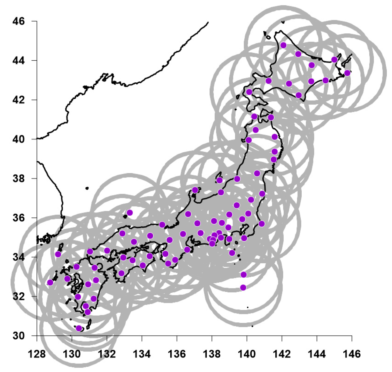
Figure 2 shows a daily graph of the number of working stations. A seismic station is considered operational for the current day if there are no gaps during that day.
3. Seismic Noise Statistics
The minimum entropy of a time series is determined by the formula , where , are the wavelet coefficients of the signal decomposition, and is the total number of coefficients . Seventeen orthogonal Daubechies wavelets were used: 10 ordinary minimum support bases with a number of zeroed moments from 1 to 10 and 7 so-called Daubechies symlets [13] with a number of vanishing moments from 4 to 10. In each time window, the wavelet for which the value is minimal is selected.
The Donoho-Johnston (DJ) wavelet-based index is the ratio of “large” wavelet coefficients in absolute value to their total number. By definition . The threshold separating “large” wavelet coefficients is , where is a robust estimate of the standard deviation of the normal distribution, are the wavelet coefficients at the first detail level of decomposition, and is the number of such coefficients [13,14].
The singularity spectrum support width is considered as a measure of the diversity of the stochastic behavior of the signal . It is defined as , where and are the minimum and maximum values of the Hölder-Lipschitz exponent [15], which governs the behavior of the signal in the vicinity of the time instant : . For a monofractal signal, the exponent is the same for all time instants . If this exponent differs, then the signal is multifractal [16].
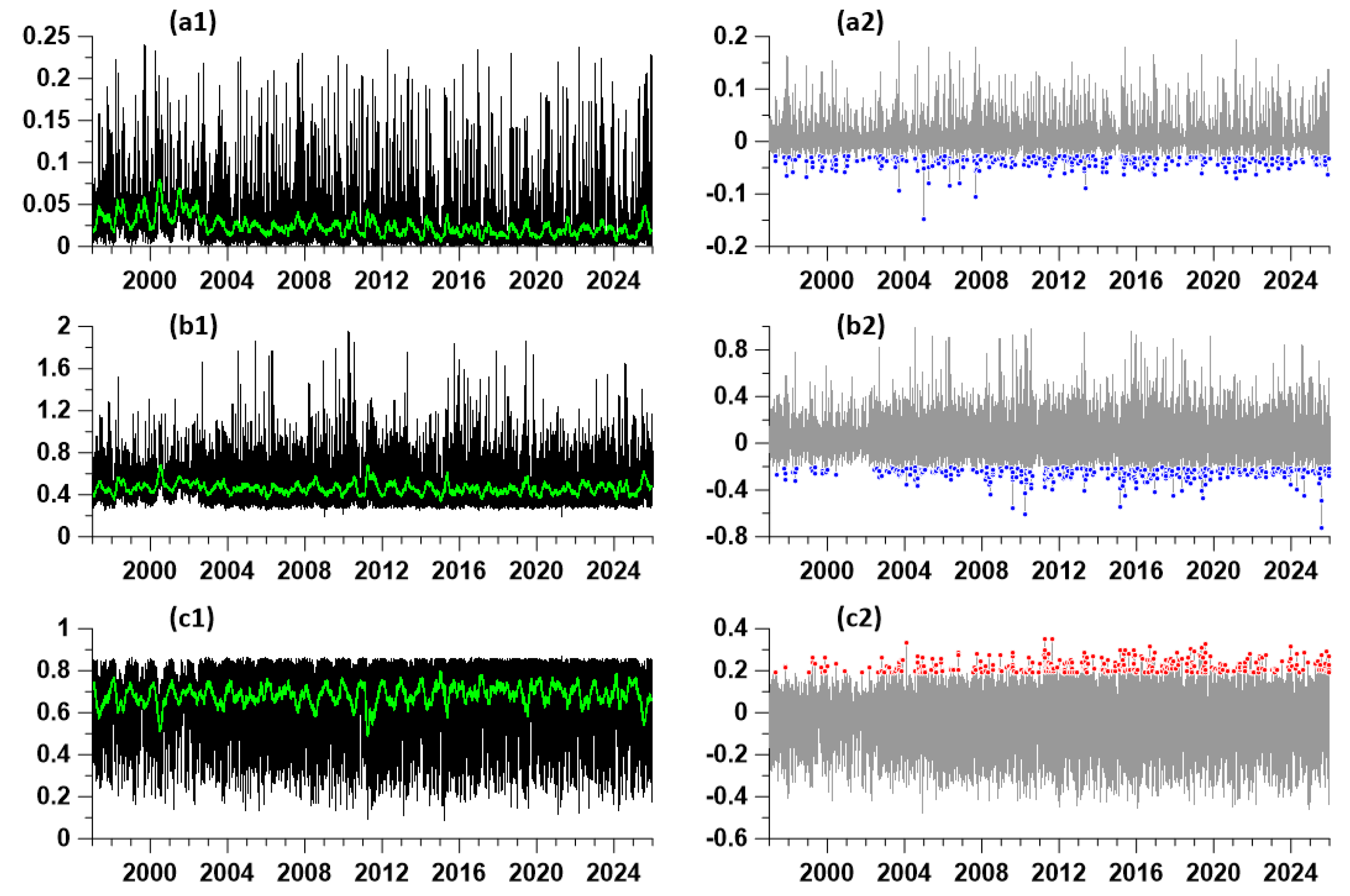
After switching to a 1-minute sampling time step, the seismic records from each station were divided into 1-day-long time fragments (1440 samples), and the parameters of daily seismic noise signals were calculated for each fragment. The methods for estimating the parameters , and for seismic noise records in a sliding time window are described in detail in [4]. The DFA method [17] was used to calculate the values of the singularity spectrum carrier width. Detrending of seismic noise signals using an 8th-order polynomial was used before calculating the entropy and index in each daily time window. Thus, time series of values with a 1-day time step were obtained for each of the seismic stations. The graphs of these quantities are presented in Figure 4 (a1, b1, c1).
The entropy value used in this paper, defined through the coefficients of the orthogonal wavelet decomposition, has features in common with multiscale entropy used, for example, in biology [18,19]. In [20,21], entropy is used within the framework of the natural time approach for seismic data analysis. In [22,23], non-extensive Tsallis entropy is used for processing seismic noise data.
The use of multifractal analysis to study the behavior of various complex systems has a long history. Particular attention is paid to the effect of parameter reduction (loss of multifractality) preceding changes in system properties. In medicine, a decrease in the value of various parameters accompanies age-related changes [24,25,26]. In [27,28], multifractal analysis is used to analyze geoelectric signals and wind speed. Within the framework of the natural time approach, multifractal analysis is used to study both seismicity and other time sequences [29,30].
In the future, we will be interested in the positions of the time points of a certain number of the largest local maxima or the smallest local minima of daily seismic noise properties in comparison with the times of earthquakes with a magnitude of at least 6 (Figure 3). To eliminate the influence of low-frequency components of changes in statistical values on the determination of the times of local extrema, the time series of noise properties were subjected to the operation of removing low frequencies using Gaussian kernel smoothing. Let be a time series with discrete time . Gaussian kernel averaging of a time series with radius (scale parameter) at time , is calculated using the formula [31]:
Next, the average values of the time series for an averaging radius of 2 days were subtracted from the time series of statistical changes, and the most significant local extremum points were found for the residuals. These operations are illustrated by the graphs in Figure 4 (a2, b2, c2).
Figure 3.
Time sequence of 352 earthquakes with magnitude of at least 6 in the rectangular vicinity of the Japanese islands (Figure 1) for the time period 1997-2025. Data source [12].
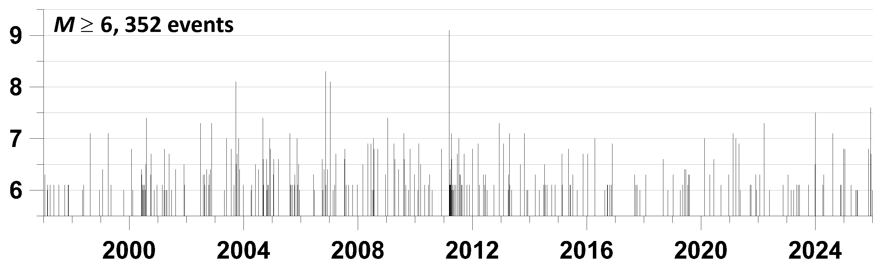
Figure 4.
Figures (a1), (b1), (c1) present the graphs of daily median values of the Donoho-Johnston index , the singularity spectrum support width , and the entropy , respectively. The green lines represent the moving averages in a 57-day window. The gray lines in figures (a2), (b2), (c2) represent the result of removing local trends with a Gaussian smoothing window of radius 2 days for the curves presented in figures (a1), (b1), (c1). The blue dots in figures (a2) and (b2) represent the 352 smallest local minima of the values and after removing local trends; the red dots in figure (c2) represent the 352 largest local maxima of the entropy values after removing local trends. The number 352 is the number of earthquakes with a magnitude of at least 6 in the rectangular area shown in Figure 1, 1997-2025 (Figure 3).
Let’s consider how the time points of the most significant local extrema of the statistics , and are distributed. To do this, we combine all the extremum points (352 smallest local minima , and 352 largest local maxima of entropy ) into a single time sequence, sort it in ascending order, and calculate the empirical probabilities of time values falling within successive six-month intervals; that is, we calculate a probability histogram of time points. Since the total length of observations is 29 years, the number of such intervals is 58. Figure 5 shows a graph of this histogram. It shows that the last six-month interval has the highest empirical probability of containing local extremum points.
4. Lead Times Between Local Extremes of Seismic Noise Properties and Earthquakes
To quantitatively estimate the relative positions of time points of local extrema of seismic noise properties and earthquake times, a measure of the mutual advance of point processes, proposed in [32] for the multivariate case, is used. For the particular case of joint processing of two point processes, this method was used in [5,34,35,36,37,38] to analyze the relationships between seismic noise properties, fluctuations of the global magnetic field, GPS tremor of the Earth’s surface, properties of the solar proton flux, and anomalies of meteorological parameters with the seismic process.
The lead measure is calculated using a parametric model of the intensity of two interacting point processes. Let represent the time instants of two event streams. Let their intensities be represented as:
where are the parameters, is the influence function of events of the flow with number :
According to formula (3), the weight of event number becomes nonzero for times and decays with characteristic time . The parameter determines the degree of influence of the event stream on the stream . The parameter determines the degree of influence of the stream on itself (self-excitation), and the parameter reflects the purely random (Poisson) component of intensity. Let us fix the parameter and consider the problem of determining the parameters .
The log-likelihood function for a non-stationary Poisson process is equal to over the time interval [39]:
It is necessary to find the maximum of functions (4) with respect to parameters . It can be shown [32,37] that problem (4) is reduced to a maximization problem
where , , , under restrictions:
Having solved the problem (5-6) numerically for a given , we can introduce the elements of the influence matrix according to the formulas:
The quantity is the portion of the average intensity of the process with index , which is purely stochastic, the portion caused by self-excitation , and the portion caused by external influence . As a result, the influence matrix can be determined:
The first column of matrix (8) is composed of Poisson fractions of mean intensities. The diagonal elements of the right-hand 2×2 submatrix consist of self-excited elements of mean intensity, while the off-diagonal elements correspond to mutual excitation. The sums of the component rows of influence matrix (8) are equal to 1. The influence matrices are estimated over a sliding time window of length with an offset and with a given value of the attenuation parameter .
Next, optimization is performed with respect to the parameters , with the aim of maximizing the average value of the difference , where is the portion of the intensity of the earthquake sequence (the first process) caused by the “influence” of the sequence of local extrema (the second process), and is the portion of the intensity of the sequence of local extrema caused by the leading influence of seismic events. We will agree to call the “direct” lead, and the “reverse” lead. The greater the difference , the greater the effect of the leading of the local extrema by the time instants relative to the time instants of the earthquakes. The problem of finding the maximum is solved within an a priori range of parameter variations: , . The values , , , , were used in the calculations; all time units are in years. The shift of the time windows was taken equal to 0.05 years. The Table 1 presents parameters of the model (2-3) which were obtained after solving the problem .
times.
Figure 6 shows graphs of changes in the values of and for points of local extrema of the analyzed properties of seismic noise with the optimal choice of parameters.
Let us denote by the result of averaging the measures of “forward” advance for various properties of seismic noise, presented by the graphs in Figure 6 ((a1), (b1), (c1)). This averaging is realized by calculating the Gaussian means of the union of these dependencies using formula (1) for an averaging radius equal to 10 days and for a uniform sequence of time points with a step of 10 days. Next, we calculate the same result of averaging the measures of “reverse” advance, presented by the graphs in Figure 6 ((a2), (b2), (c2)). Figure 7 shows their difference as a function of the position of the right end of successive time intervals of 10 days.
The value is an integrated measure of the lead time of local extrema in seismic noise properties relative to the times of earthquakes with magnitudes of at least 6. The vertical blue line in Figure 7 represents the time of the Tohoku mega-earthquake of March 11, 2011. The graph in Figure 7 shows that this measure is mostly positive; that is, for most times, the points of local extrema in seismic noise properties lead the times of earthquakes. An exception is a time interval of just under 4 years, adjacent to the time of the Tohoku event on the right and extending to the 2015 time stamp, when the value is negative. The graph in Figure 7 also shows other time segments when , but they are not as long as after the Tohoku earthquake. The time intervals correspond to a situation when, on average, the attainment of extreme values of properties , and is a consequence of earthquakes. If , then this means that local extremes of noise properties foreshadow seismic events.
For two long time periods before the Tohoku event and after the 2015 timestamp, quasi-periodic fluctuations in the measure values are noticeable. We estimate their periods by fitting harmonic oscillations (shown as green lines in Figure 7) using the least-squares method with unknown periods, which we find by minimizing the residual variance. It turns out that these periods are quite close to each other, equal to 3.5 years before the Tohoku event and 3.2 years after 2015.
5. The First Principal Components of the Amplitudes of the EEMD Envelope Decompositions of Seismic Noise Properties
Let us consider the issue of identifying the general fluctuations of the median values of the noise properties , and , the graphs of which are presented in Figure 4 ((a1), (b1), (c1)). To solve this problem, we will use the Hilbert-Huang method [40,41] of decomposing signals into sequences of intrinsic mode functions (IMF), also known as empirical mode decomposition (EMD). The use of EMD decomposition has a wide range of applications. In [29], this method was used to analyze seismicity on various time scales in combination with multifractal analysis. In [35,37], EEMD decomposition was used to analyze the prognostic properties of GPS tremor of the earth’s surface and anomalies of meteorological time series.
The decomposition of an arbitrary signal into empirical oscillation modes is given by the formula:
where is the j-th empirical mode, is the remainder, and n is the number of empirical modes.
The algorithm for decomposing into a sequence of empirical modes is iterative for each level . We denote by the iteration index, where is the maximum number of iterations for level . The iterations are described by the formula
Here , where and are the upper and lower envelopes for the signal , which are constructed using spline interpolation (usually a 3rd order spline) over all local maxima and minima of the signal .
Iterations (10) are initialized with a zero step for the first level () of the decomposition . Next, the upper and lower envelopes and are found, the mean line is calculated, and is found using formula (10). For , the upper and lower envelopes and are determined, and the mean line are found, and so on, up to the last iteration index , after which the first empirical mode is considered to have been found.
The condition for stopping the iterations is usually chosen in the form of the inequality:
where is some small number, such as 0.01. Once the mode is found, an iterative process is started to determine the empirical mode of the next level. This process is initialized by the formula for the initial iteration index :
According to formula (12), the high-frequency component is subtracted from the original signal, and the resulting lower-frequency signal is considered a new signal for subsequent decomposition. The construction of empirical oscillation modes continues until the number of local extrema becomes too small to be used to construct envelopes.
As the empirical mode level number increases, the signals become increasingly low-frequency and tend toward an unchanging form. The sequence is constructed such that its sum yields an approximation of the original signal, which can be represented as (9).
Empirical oscillation modes, known as Intrinsic Mode Functions (IMFs), are orthogonal to each other, thus forming the empirical basis for decomposing the original signal. From here on, these decomposition levels will be referred to as IMF levels.
One of the drawbacks of the EMD method is the problem of mode mixing, which occurs when a single empirical mode includes signals of different scales or when signals of the same scale are distributed across different empirical modes. For example, if a signal exhibits “intermittency,” meaning that short-lived sections of higher-frequency behavior appear against a smooth background, then EMD decomposition results in a mixing of modes with different frequencies, as the relatively rare local extrema of the smooth behavior are interspersed with significantly more frequent local extrema of the high-frequency component.
To combat this effect, the ensemble empirical mode decomposition (EEMD) method was proposed in [41]. It is a regularization of the EMD method, in which finite-amplitude white noise is added to the original data. This allows the true empirical modes to be determined as the average value over an ensemble of trials, each of which is the sum of the signal and white noise.
The EEMD algorithm includes the following steps:
- Adding a white noise realization to the original data.
- Decomposing the data with the added white noise into empirical modes.
- Repeating steps 1 and 2 a sufficiently large number of times with independent white noise realizations.
- Obtaining the ensemble mean for the corresponding empirical modes.
Thus, numerous artificial observations are simulated in real time series:
where is the i-th realization of white noise. In our calculations, we used 1000 realizations of independent white noise with a standard deviation equal to 0.1 of the standard deviation of the original signals.
After obtaining EEMD realizations of daily time series of noise properties , and for a sequence of IMF levels, we calculate the amplitudes of their envelopes using the Hilbert transform, which is efficiently implemented using the fast Fourier transform [42]. For each IMF level, we have 3 time functions of the envelope amplitudes corresponding to different properties of seismic noise. To isolate their common properties at each level, we calculate their first principal component after centering and normalization to unit variance [43,44]. The graphs of the first principal components of the envelope amplitudes are presented in Figure 8 for the first 8 IMF levels of the EEMD decomposition. Each IMF level approximately corresponds to a frequency band with boundary periods from to , where is the IMF level number, is the time sampling step (in our case, 1 day).
Among the graphs in Figure 8, the low-frequency IMF levels 5-8 are particularly striking. At IMF levels 5-7, peaks in the first principal component centered on the time of the Tohoku mega-earthquake of March 11, 2011, are visible, indicating a post-seismic response. However, the IMF level 8 graph (periods from 256 to 512 days) displays a significant peak for the time interval from mid-2024 to late 2025, which may indicate preparation for the next strong earthquake.
6. Probability Densities of Extreme Values of Seismic Noise Properties
Let us study the variability of the spatial distribution of extreme values of seismic noise properties. For this purpose, we consider a regular grid of 30×30 nodes, covering an area with latitude from 28°N to 46°N and longitude from 128°E to 146°E (Figure 1). Let be any value of , or . For each grid node and for each day with number , we find the 5 nearest working seismic stations, which yields 5 values of . Let us denote by the median value of these 5 properties at a node on a day with number . The values in the set of nodes of the regular grid can be considered as an elementary daily map. For each daily elementary map with a discrete time index , we find the coordinates of the nodes at which a given number of extreme values of is reached relative to all other nodes of the regular grid. Minima are found for or , and maxima are found for . Further, extreme values will be used. The set of two-dimensional vectors considered within the time interval forms a random set. We estimate the two-dimensional probability distribution function of the vectors for each node of the regular grid. For each node , the probability density function of the distribution of extreme values of the property is calculated according to the Parzen-Rosenblatt estimate with the Gaussian kernel function [44]:
Here is the kernel averaging radius, are integer indices that number the daily elementary maps, and is the number of daily maps in the time interval under consideration. A smoothing bandwidth of was used.
Let us calculate the 2-dimensional distribution densities (14) of extreme values in successive time windows of 10 days in length (). Since we have three such distributions, we will calculate their weighted average by taking as weights the squares of the components of the eigenvector of the correlation matrix of probability densities corresponding to the maximum eigenvalue of the matrix [43]. By construction, the sum of the squares of the components is equal to 1. Figure 9 shows graphs of the weighting coefficients depending on the position of the right end of time windows of 10 days in length.
To quantitatively describe the sequence of values of the weighted probability density function (PDF) for the distribution of extreme seismic noise properties in 10-day time windows, we consider the entropy of these densities. Let be the number of grid nodes within the region formed by the union of circles with a radius of 250 km, centered at each F-net station (Figure 1). We calculate the histogram of the weighted probability density functions for each 10-day interval as a sequence of values:
where is the number of intervals dividing the range of density variation within a given 10-day window into intervals of equal length. According to recommendations [31,44], we choose the value . Obviously , the values of the histogram (15) also have the properties of a discrete probability distribution. We define the normalized entropy of this distribution by the formula:
In Figure 10, the gray line represents the graph of entropy change (16) depending on the position of the right end of 10-day time windows. The red line represents the result of smoothing with a Gaussian kernel (formula (1)) with a smoothing kernel width of 400 days.
The blue line represents a stepwise approximation using so-called long WTMM (Wavelet Transform Modulus Maxima) chains of the signal skeleton. Scale-dependent stepwise approximation allows one to formally determine the moments in time of significant changes in the mean entropy values. This approximation is constructed using continuous wavelet transforms with a kernel in the form of derivatives of a Gaussian function, which allows one to formalize the selection of moments in time at which a significant, scale-dependent change in the mean value of a noisy signal occurs [13,45].
To describe the construction of the stepwise WTMM approximation, we will use continuous-time formulas, which are easily adapted to the discrete-time case but are more compact. The smoothed entropy value is calculated using the formula:
where is the smoothing time scale. For the -th derivative of the smoothed signal, divided by (the Taylor coefficient), the following expression holds:
where . A two-dimensional WTMM point for is defined as a point for which exhibits a local maximum in time for a given time scale . For , WTMM points are defined as points of local extrema (maxima or minima) of the smoothed signal , which can be combined into chains. The set of all chains forms the WTMM skeleton of the signal. If the kernel is Gaussian, then a given chain of the WTMM skeleton does not terminate (does not “hang in the air”) when decreasing the scale and touches the time axis [46]. The WTMM points for the 1st-order derivative indicate the time points of maximum trend (positive or negative) of the smoothed signal for a given scale . This can be used to formally identify points of large changes in the mean. These times correspond to the roots of long WTMM chains reaching given values of the scale . We define a stepwise WTMM approximation for a signal as a function that is equal to a sequence of constant values in successive intervals . Here denote the beginnings of WTMM chains for , which exceed a threshold time scale and stepwise approximation is equal to the sequence of average values within the time intervals .
In Figure 10, the blue line represents the stepwise WTMM approximation for the parameter days. This threshold time scale ensures that the overall time interval is divided into 12 fragments with different average entropy values, which are then interpreted as stages in the development of seismic noise field features in the Japanese islands. A comparison of the red and blue lines in Figure 10 shows that both averaging methods exhibit roughly the same behavior in the most general trends. In particular, the final time interval from the end of 2020 is characterized by elevated average entropy values.
7. A Sequence of Distribution Maps of Average-Weighted Probability Densities of Extreme Values of Noise Properties
Figure 11 shows a sequence of distributions of average-weighted probability densities of extreme values of seismic noise properties in the region of the Japanese islands in the union of circles with a radius of 250 km, constructed around each seismic station for 12 time intervals allocated by the stepwise WTMM approximation of entropy (16).
Within the framework of the considered hypothesis, the areas of concentration of the weighted probability density are interpreted as “spots of increased seismic hazard.” The time intervals identified by the stepwise approximation of entropy (16) can be represented as a sequence of 12 stages of precursor development based on the properties of seismic noise. The first six distribution maps (α01-α06) correspond to the time intervals preceding the Tohoku event, the epicenter of which is shown by a black asterisk. In the first two maps (α01, α02), it is noticeable how a single area of concentration of the probability density at α01 splits into two parts, one of which at α02 closely approaches the epicenter of the Tohoku event. Stage α03 lasts for approximately six months, and during this short period of time, for which the average entropy value (16) declines, a region of probability density concentration formed in the region of 30°N≤Lat≤34°N, 136°E≤Lon≤140°E, which remains stable for all later stages. A clear precursor to the future Tohoku mega-earthquake of March 11, 2011, formed during stages (α04-α06). Note the significant duration of the time interval corresponding to stage α06.
Five stages (α07-α11) demonstrate a relatively calm evolution of “seismic hazard spots” with periodic moderate concentration of probability density in the Tohoku aftershock region, the bursts of which correspond to an increase in the average entropy values (16) in Figure 10. Finally, the last stage α12 is characterized by a significant rearrangement of the configuration of seismic hazard spots. Concentration of probability density is observed along the entire length of the Pacific coast of Japan (subduction region), while the area of the highest density values remains low-lying in the region 30°N≤Lat≤34°N, 136°E≤Lon≤140°E. During stage α12, the Aomori earthquake occurred on December 8, 2025, M=7.6, the epicenter of which is shown by a black asterisk on the α12 map.
8. Conclusions
A method for analyzing the evolution of low-frequency seismic noise field properties in a seismically active region is proposed. This method is based on studying the temporal and spatial distribution of extreme values of noise properties, which describe the complexity of its statistical structure. An increase in seismic hazard is interpreted as a simplification of the noise structure and its approach to the properties of white noise, as well as the synchronization of temporal variations in these properties. A method for identifying stages in the development of a seismic noise field is proposed based on a stepwise WTMM approximation of the change in the entropy of the distribution of weighted average densities of the distribution of extreme values of seismic noise properties. The method is applied to the analysis of noise properties on the Japanese islands over 29 years of observations, 1997-2025.
The main conclusions are that the spatial and temporal behavior of low-frequency seismic noise properties in Japan since 2020, and particularly in the last two years, reveal a number of indicators that point to the preparation of the next strong earthquake. Figure 5 shows a spike in the probability histogram of the distribution of time points when the values of the properties under consideration reach extreme values over the last six months. Figure 7 shows a pattern of quasi-periodic oscillations in the average integrated measure of the lead time of seismic noise property extreme points relative to the time points of strong earthquakes with a magnitude of at least 6 since 2015, with a peak value at the end of 2025, following a four-year interval when this pattern disappeared following the Tohoku mega-earthquake of March 11, 2011. Figure 8 shows a spike in the first principal component of the envelope amplitudes for the EEMD Hilbert-Huang decomposition of the daily median values of three seismic noise properties for the lowest-frequency IMF level number 8 (characteristic periods from 256 to 512 days) for the 2024-2025 time interval. This spike indicates synchronization of low-frequency variations in seismic noise properties. Figure 10 shows that the average entropy values of the weighted average probability density distribution of noise property extremes reach their maximum values from the end of 2020 to the end of 2025. Figure 11, which visualizes 12 stages of seismic noise field development on the Japanese islands, shows that the situation before the Tohoku mega-earthquake (stages (α04-α06)) is repeated at the final stage, α12, in that new “seismic hazard” spots appear, covering the entire Pacific coast of Japan. At the same time, the maximum probability density in the southern part of the studied area of the Japanese islands, which formed at stage α03, remains stable.
Taken together, these features are interpreted as indicators of increased current seismic hazard, with particular attention to the region 30°N≤Lat≤34°N, 136°E ≤Lon≤140°E. Naturally, this is not a prediction of the timing of the next strong earthquake; the essence of this study is to detect a trend of increasing seismic hazard.
Author Contributions
A.L.—ideating the research, writing the text, and data processing.
Funding
This research received no external funding.
Institutional Review Board Statement
Not applicable.
Informed Consent Statement
Not applicable.
Data Availability Statement
The original seismic data are contained in the database at http://www.fnet.bosai.go.jp/faq/?LANG=en (accessed on 04 January 2026). Information about seismic processes was taken from https://earthquake.usgs.gov/earthquakes/search (accessed on 04 January 2026).
Acknowledgments
This work was carried out within the framework of the state assignments of the Institute of Physics of the Earth of the Russian Academy of Sciences.
Conflicts of Interest
The authors declare that the research was conducted in the absence of any commercial or financial relationships that could be construed as potential conflicts of interest.
References
- Lyubushin, A.A. Dynamic estimate of seismic danger based on multifractal properties of low-frequency seismic noise. Natural Hazards 2014, 70, 471–483. [Google Scholar] [CrossRef]
- Lyubushin, A. Synchronization of Geophysical Fields Fluctuations. In Complexity of Seismic Time Series: Measurement and Applications;Chapter 6; Chelidze, Tamaz, Telesca, Luciano, Vallianatos, Filippos, Eds.; Elsevier: Amsterdam, Oxford, Cambridge, 2018; pp. P.161–197. [Google Scholar] [CrossRef]
- Lyubushin, A.A. Seismic Noise Wavelet-Based Entropy in Southern California. Journal of Seismology 2020. [Google Scholar] [CrossRef]
- Lyubushin, A. Low-Frequency Seismic Noise Properties in the Japanese Islands. Entropy 2021, 23, 474. [Google Scholar] [CrossRef]
- Lyubushin, A. Seismic Hazard Indicators in Japan based on Seismic Noise Properties. J. Earth Environ. Sci. Res. 2023, 5, 1–8. [Google Scholar] [CrossRef]
- Rikitake, T. Probability of a great earthquake to recur in the Tokai district, Japan: reevaluation based on newly-developed paleoseismology, plate tectonics, tsunami study, micro-seismicity and geodetic measurements. Earth, Planets and Space 1999, 51, 147–157. [Google Scholar] [CrossRef]
- Mogi, K. Two grave issues concerning the expected Tokai Earthquake. Earth, Planets and Space 2004, 56, li–lxvi. [Google Scholar] [CrossRef]
- Simons, M.; Minson, S.E.; Sladen, A.; Ortega, F.; Jiang, J.; Owen, S.E. The 2011 Magnitude 9.0 Tohoku-Oki earthquake: mosaicking the megathrust from seconds to centuries. Science 2011, 332, 911. Available online: https://science.sciencemag.org/content/332/6036/1421. [CrossRef]
- Kagan, Y.Y.; Jackson, D.D. Tohoku Earthquake: A Surprise? Bulletin of the Seismological Society of America 2013, 103, 1181–1194. [Google Scholar] [CrossRef]
- Zoller, G.; Holschneider, M.; Hainzl, S.; Zhuang, J. The largest expected earthquake magnitudes in Japan: the statistical perspective. Bull. Seismol. Soc. Am. 2014, 104, 769–779. [Google Scholar] [CrossRef]
- Broadband Seismograph Network NIED F-net. Available online: http://www.fnet.bosai.go.jp/faq/?LANG=en (accessed on 4 January 2026).
- USGS Search Earthquake Catalog. Available online: https://earthquake.usgs.gov/earthquakes/search/ (accessed on 4 January 2026).
- Mallat, S.A. Wavelet Tour of Signal Processing, 2nd edition; Academic Press: San Diego, London, Boston, New York, Sydney, Tokyo, Toronto, 1999. [Google Scholar]
- Donoho, D.L.; Johnstone, I.M. Adapting to unknown smoothness via wavelet shrinkage. J. Am. Stat. Assoc. 1995, 90, 1200–1224. [Google Scholar] [CrossRef]
- Taqqu, M.S. Self-similar processes. In Encyclopedia of Statistical Sciences; Wiley: New York, NY, 1988; vol.8, pp. 352–357. [Google Scholar]
- Feder, J. Fractals; Plenum Press: New York, London, 1988. [Google Scholar]
- Kantelhardt, J.W.; Zschiegner, S.A.; Konscienly-Bunde, E.; Havlin, S.; Bunde, A.; Stanley, H.E. Multifractal detrended fluctuation analysis of nonstationary time series. Phys. A 2002, 316, 87–114. [Google Scholar] [CrossRef]
- Costa, M.; Peng, C.-K.; Goldberger, A.L.; Hausdorf, J.M. Multiscale entropy analysis of human gait dynamics. Physica A 2003, 330, 53–60. [Google Scholar] [CrossRef] [PubMed]
- Costa, M.; Goldberger, A.L.; Peng, C.-K. Multiscale entropy analysis of biological signals. Phys. Rev. 2005, E 71, 021906. [Google Scholar] [CrossRef]
- Varotsos, P.A.; Sarlis, N.V.; Skordas, E.S.; Lazaridou, M.S. Entropy in the natural time domain. Phys. Rev. E 2004, 70, 011106. [Google Scholar] [CrossRef]
- Varotsos, P.A.; Sarlis, N.V.; Skordas, E.S. Natural Time Analysis: The New View of Time. In Precursory Seismic Electric Signals, Earthquakes and other Complex Time Series; Springer-Verlag Berlin Heidelberg, 2011. [Google Scholar] [CrossRef]
- Koutalonis, I.; Vallianatos, F. Evidence of Non-extensivity in Earth’s Ambient Noise. Pure Appl. Geophys. 2017, 174, 4369–4378. [Google Scholar] [CrossRef]
- Vallianatos, F.; Koutalonis, I.; Chatzopoulos, G. Evidence of Tsallis entropy signature on medicane induced ambient seismic signals. Physica A 2019, 520, 35–43. [Google Scholar] [CrossRef]
- Ivanov, P. Ch; Amaral, L.A.N.; Goldberger, A.L.; Havlin, S.; Rosenblum, M.B.; Struzik, Z. Multifractality in healthy heartbeat dynamics. Nature 1999, 399, 461–465. [Google Scholar] [CrossRef]
- Humeaua, A.; Chapeau-Blondeau, F.; Rousseau, D.; Rousseau, P.; Trzepizur, W.; Abraham, P. Multifractality, sample entropy, and wavelet analyses for age-related changes in the peripheral cardiovascular system: preliminary results. Med. Phys., Am. Assoc. Phys. Med. 2008, 35, 717–727. [Google Scholar] [CrossRef]
- Dutta, S.; Ghosh, D.; Chatterjee, S. Multifractal detrended fluctuation analysis of human gait diseases. Front. Physiol. 2013, 4, 274. [Google Scholar] [CrossRef] [PubMed]
- Telesca, L.; Colangelo, G.; Lapenna, V. Multifractal variability in geoelectrical signals and correlations with seismicity: a study case in southern Italy. Nat. Hazard. Earth Syst. Sci. 2005, 5, 673–677. [Google Scholar] [CrossRef]
- Telesca, L.; Lovallo, M. Analysis of the time dynamics in wind records by means of multifractal detrended fluctuation analysis and the Fisher-Shannon information plane. J. Stat. Mech. 2011, P07001. Available online: https://iopscience.iop.org/article/10.1088/1742-5468/2011/07/P07001. [CrossRef]
- Sarlis, N.V.; Skordas, E.S.; Mintzelas, A.; Papadopoulou, K.A. Micro-scale, mid-scale, and macro-scale in global seismicity identified by empirical mode decomposition and their multifractal characteristics. Scientific Reports 2018, 8, 9206. [Google Scholar] [CrossRef]
- Mintzelas, A.; Sarlis, N.V.; Christopoulos, S.-R.G. Estimation of multifractality based on natural time analysis. Physica A 2018, 512, 153–164. [Google Scholar] [CrossRef]
- Hardle, W. Applied Nonparametric Regression. In Biometric Society Monographs No. 19; Cambridge University Press: Cambridge, 1990. [Google Scholar]
- Lyubushin, A.A.; Pisarenko, V.F. Research on Seismic Regime Linear Model of Intensity of Interacting Point Processes. Phys. Solid. Earth Engl. Transl. 1994, 29, 1108–1113. [Google Scholar]
- Lyubushin, A. Investigation of the Global Seismic Noise Properties in Connection to Strong Earthquakes. Front. Earth Sci. 2022, 10, 905663. [Google Scholar] [CrossRef]
- Lyubushin, A.; Rodionov, E. Wavelet-based correlations of the global magnetic field in connection to strongest earthquakes. Adv. Space Res. 2024, 74, 3496–3510. [Google Scholar] [CrossRef]
- Lyubushin, A.; Rodionov, E. Prognostic Properties of Instantaneous Amplitudes Maxima of Earth Surface Tremor. Entropy 2024, 26, 710. [Google Scholar] [CrossRef]
- Lyubushin, A.; Rodionov, E. Quantitative Assessment of the Trigger Effect of Proton Flux on Seismicity. Entropy 2025, 27, 505. [Google Scholar] [CrossRef] [PubMed]
- Lyubushin, A.; Kopylova, G.; Rodionov, E.; Serafimova, Y. An Analysis of Meteorological Anomalies in Kamchatka in Connection with the Seismic Process. Atmosphere 2025, 16, 78. [Google Scholar] [CrossRef]
- Lyubushin, A.; Rodionov, E. The Relationship Between the Seismic Regime and Low-Frequency Variations in Meteorological Parameters Measured at a Network of Stations in Japan. Atmosphere 2025, 16, 1129. [Google Scholar] [CrossRef]
- Cox, D.R.; Lewis, P.A.W. The Statistical Analysis of Series of Events; Methuen: London, UK, 1996. [Google Scholar]
- Huang, N.E.; Shen, Z.; Long, S.R.; Wu, V.C.; Shih, H.H.; Zheng, Q.; Yen, N.C.; Tung, C.C.; Liv, H.H. The empirical mode decomposition and the Hilbert spectrum for nonlinear and non-stationary time series analysis. Proc. Roy. Soc. Lond. Ser. A 1998, 454, 903–995. [Google Scholar] [CrossRef]
- Huang, N.E.; Wu, Z. A review on Hilbert-Huang transform: Method and its applications to geophysical studies. Rev. Geophys. 2008, 46, RG2006. [Google Scholar] [CrossRef]
- Bendat, J.S.; Piersol, A.G. Random Data. Analysis and Measurement Procedures, 4th ed.; Wiley & Sons: Hoboken, NJ, USA, 2010. [Google Scholar]
- Jolliffe, I.T. Principal Component Analysis; Springer-Verlag, 1986. [Google Scholar] [CrossRef]
- Duda, R.O.; Hart, P.E.; Stork, D.G. Pattern Classification; Wiley-Interscience Publication: New York, Chichester, Brisbane, Singapore, Toronto, 2000. [Google Scholar]
- Mallat, S.; Zhong, S. Characterization of signals from multiscale edges. IEEE Trans Pattern Recog Mach Intell 1992, 1 4, 710–32. [Google Scholar] [CrossRef]
- Hummel, B.; Moniot, R. Reconstruction from zero-crossings in scale-space. IEEE Trans Acoust Speech Signal Process 1989, 37, 2111–2130. [Google Scholar] [CrossRef]
Figure 2.
Number of daily operating stations of the F-net network.
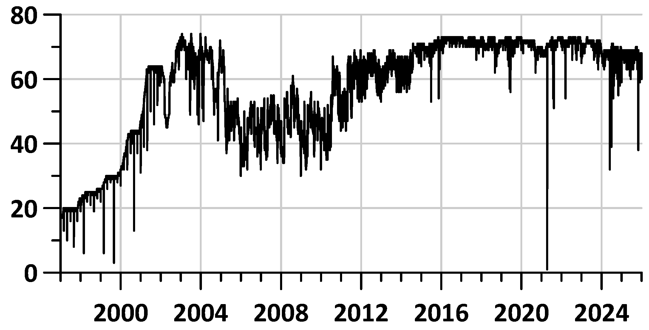
Figure 5.
Probability histogram of the time distribution of extreme values of three seismic noise properties (local entropy maxima and local minima of the singularity spectrum support width and DJ index ). For each property, the number of most significant local extreme points is taken to be 352—the number of earthquakes with magnitudes of at least 6.
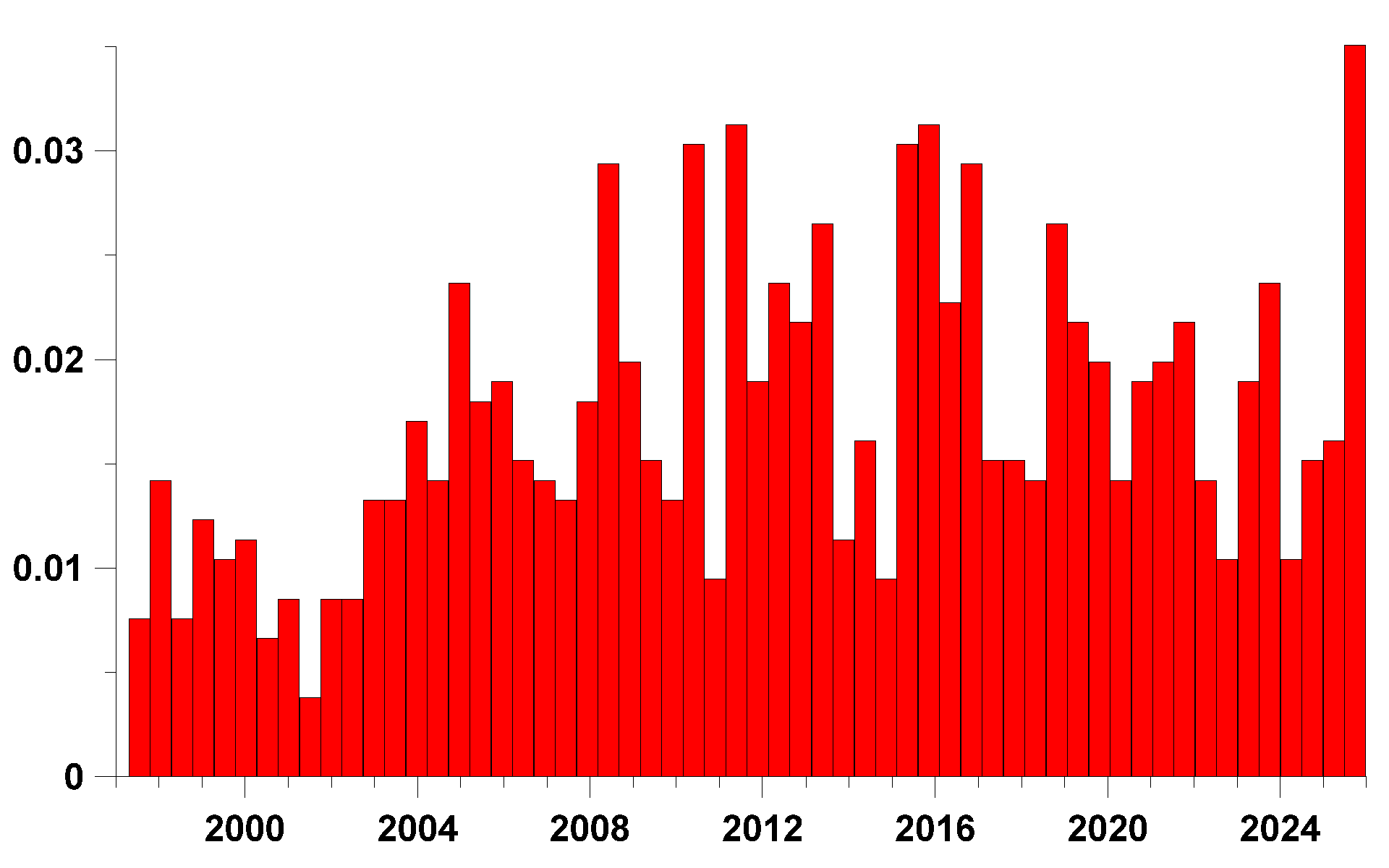
Figure 6.
Figures (a1), (b1), (c1) present graphs of the “direct” lead measures by the time points of the most pronounced local extrema of the values , and relative to the times of earthquakes with the optimal choice of the attenuation time and the length of the time window (Table 1). Figures (a2), (b2), (c2) present graphs of the “inverse” lead measures by the time points of earthquakes relative to the time points of the most pronounced local extrema of the values , and . The horizontal red lines represent the average values of the “direct” and “inverse” lead measures (Table).
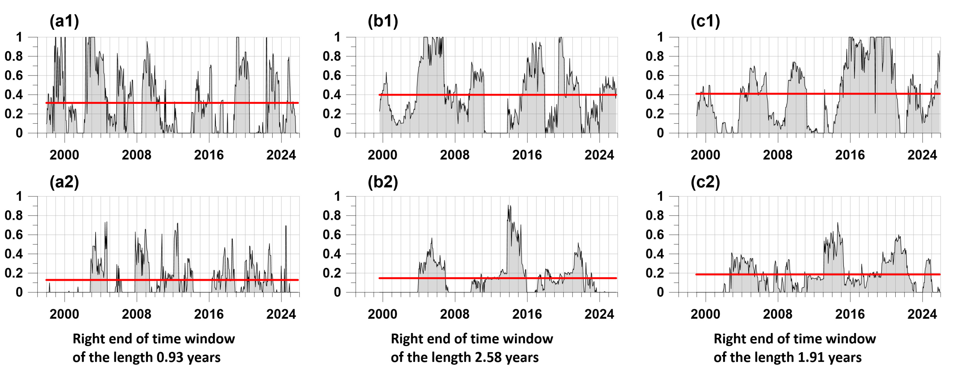
Figure 7.
Plot of the differences between the averaged forward and backward advance measures of the times of properties , and extremes relative to the times of earthquakes . The vertical blue line represents the time of the Tohoku mega-earthquake of March 11, 2011, M=9.1. The horizontal red line represents the mean of the differences in the averaged advance measures, equal to 0.224. The two green lines represent the graphs of the best approximations by harmonic oscillations of the advance measure difference for time intervals before the Tohoku event (3.5-year period) and after 2015 (3.2-year period).
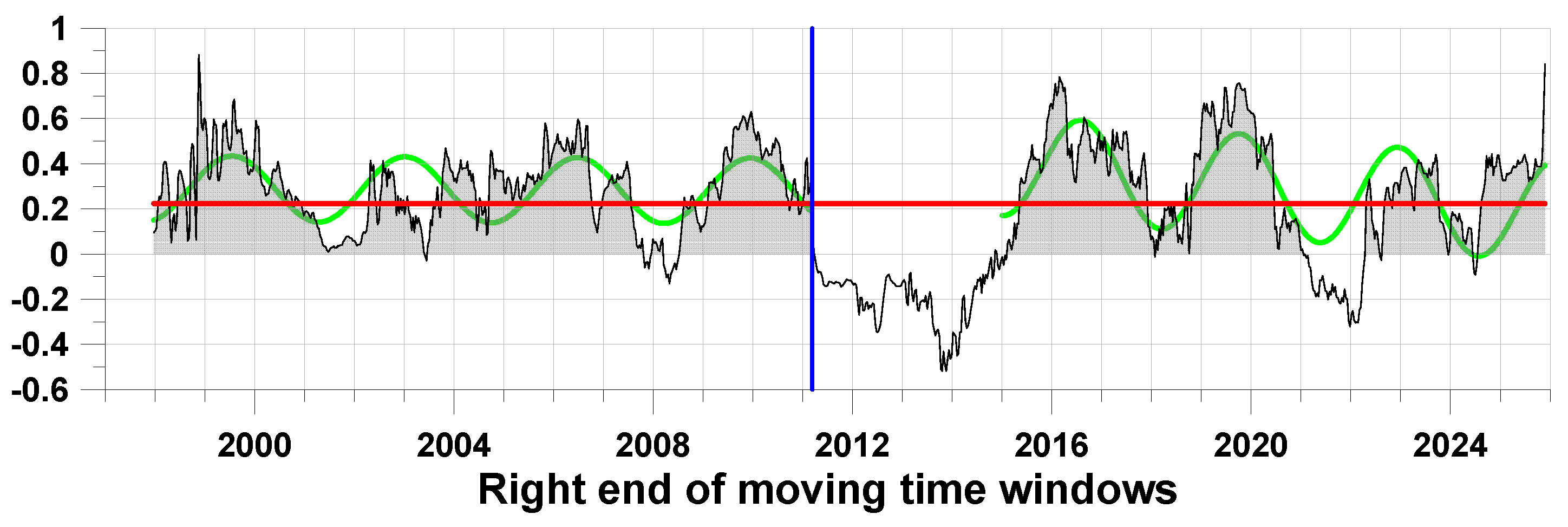
Figure 8.
Graphs of the first principal components of the amplitudes of the envelopes of the daily median values of the properties , and , calculated using the Hilbert transform for the EEMD Huang realizations at the first 8 IMF levels of the expansion into empirical oscillation modes.
Figure 8.
Graphs of the first principal components of the amplitudes of the envelopes of the daily median values of the properties , and , calculated using the Hilbert transform for the EEMD Huang realizations at the first 8 IMF levels of the expansion into empirical oscillation modes.
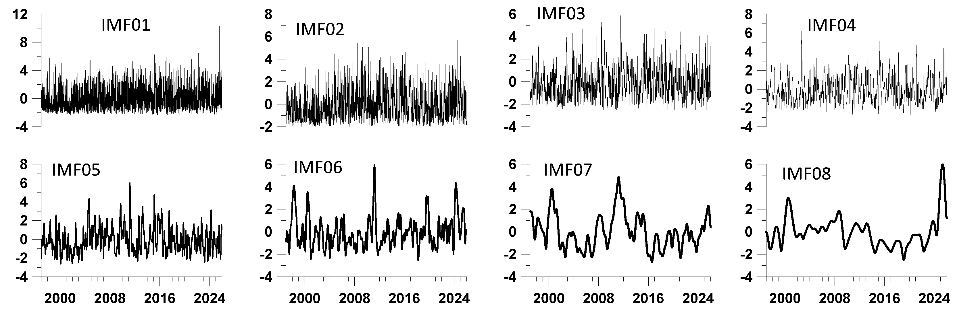
Figure 9.
Graphs of changes in the weighting coefficients used in the weighted averaging of the probability densities of the distribution of extreme values of properties , (minima) and (maxima) in successive time windows of 10 days in length.
Figure 9.
Graphs of changes in the weighting coefficients used in the weighted averaging of the probability densities of the distribution of extreme values of properties , (minima) and (maxima) in successive time windows of 10 days in length.
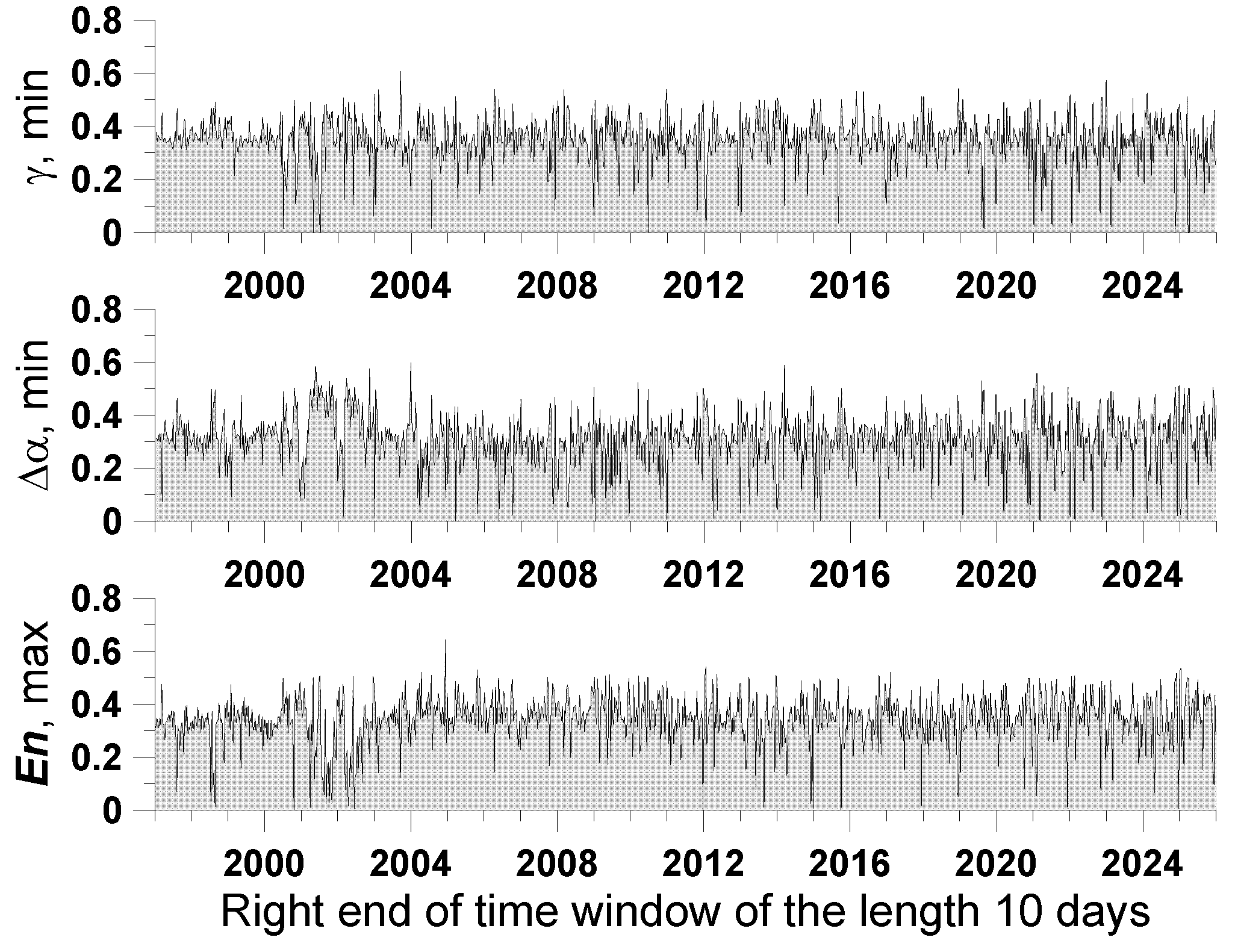
Figure 10.
The gray line represents the change in the entropy of the weighted probability density function of extreme values of properties , and , calculated in successive 10-day time windows. The blue line represents the stepwise WTMM approximation, which divides the time interval into 12 segments with different mean entropy values. The red line represents the smoothed entropy values with a Gaussian window of radius 400 days.
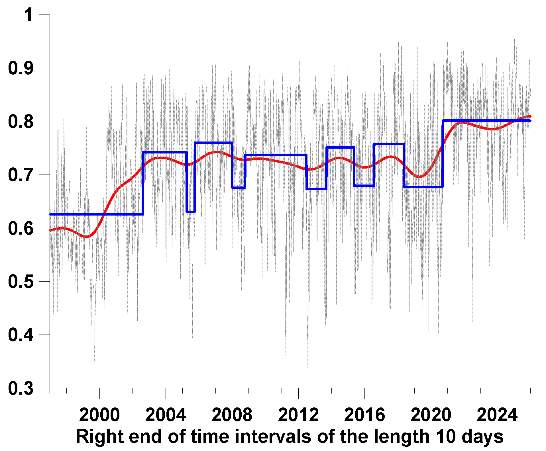
Figure 11.
The 2-dimensional weighted average probability densities of the distribution of extreme values of the properties , and , averaged over 12 time intervals identified using the stepwise WTMM approximation of entropy, are presented. The time boundaries of the intervals are indicated at the top of each 2-dimensional distribution map as fractional years. In the maps (α01-α06) for 6 time intervals before the Tohoku earthquake of March 11, 2011, M=9.1, the position of the hypocenter of this event is shown by a black asterisk. In the map (α12), the position of the hypocenter of the Aomori earthquake of December 8, 2025, M=7.6 is shown by a black asterisk.
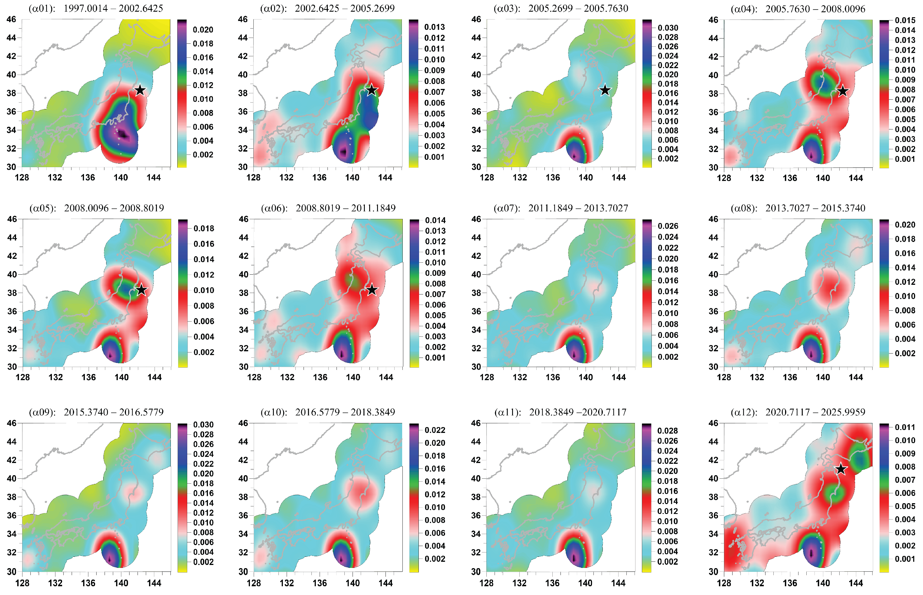

Table 1.
Values of optimal parameters of the intensity model of two related consecutive events for the extreme points of various properties of seismic noise and earthquake
Table 1.
Values of optimal parameters of the intensity model of two related consecutive events for the extreme points of various properties of seismic noise and earthquake
| Property | |||
|---|---|---|---|
| , years | 0.055 | 0.080 | 0.052 |
| , years | 0.93 | 2.58 | 1.91 |
| Mean of | 0.315 | 0.399 | 0.410 |
| Mean of | 0.129 | 0.145 | 0.186 |
| Difference | 0.186 | 0.251 | 0.224 |
Disclaimer/Publisher’s Note: The statements, opinions and data contained in all publications are solely those of the individual author(s) and contributor(s) and not of MDPI and/or the editor(s). MDPI and/or the editor(s) disclaim responsibility for any injury to people or property resulting from any ideas, methods, instructions or products referred to in the content. |
© 2026 by the authors. Licensee MDPI, Basel, Switzerland. This article is an open access article distributed under the terms and conditions of the Creative Commons Attribution (CC BY) license (http://creativecommons.org/licenses/by/4.0/).
Copyright: This open access article is published under a Creative Commons CC BY 4.0 license, which permit the free download, distribution, and reuse, provided that the author and preprint are cited in any reuse.


