
Submitted:
21 January 2026
Posted:
22 January 2026
You are already at the latest version
Abstract
Marine controlled source electromagnetic (CSEM) surveys have been proven to be an effective tool in hydrocarbon exploration, principally due to the method’s ability (in the right circumstances) to identify electrical resistivity contrasts between hydrocarbon-saturated and brine-saturated sedimentary units. However the sensitivity of such surveys decreases in shallow water, for deeper targets, and for targets with limited horizontal extent. In principle, the resolution and sensitivity of a survey can be improved by moving either the transmitting or the receiving dipoles into the sub-surface. We have therefore investigated the sensitivity of Seafloor to Borehole CSEM (sbCSEM) survey geometries, specifically for the case of targets with small lateral dimensions in shallow water areas – including targets whose depth of burial substantially exceeds their lateral extent. The results are encouraging. Neither small target size nor shallow water present obstacles in principle to the use of this approach. Our models reveal distinct lobes in the patterns of electric field and current density amplitudes around a sub-seafloor transmitting dipole. The shape, positions and amplitudes of these lobes are all strongly modified by the presence of one or more small resistive targets, and in particular are strongly influenced by the positions of target edges. These effects significantly modify the pattern of electric fields at the seafloor, and hence result in good sensitivity for realistic survey geometries. Small targets can be detected by seafloor receivers when the sub-seafloor transmitting dipole is located at some distance laterally outside the targets - leading to potential applications in ‘step-out’ prospecting. The asymmetry of responses at the seafloor from targets that are offset with respect to transmitter location has potential applications in field appraisal; while monitoring of reservoirs during production provides another possible application. Varying the depth of the transmitter down the borehole generates a Vertical EM Profiling (VEMP) survey – analogous to Vertical Seismic Profiling (VSP) – and we demonstrate that this too can have useful applications. Modelling for deeper (3 km sub-seafloor) targets continues to yield encouraging results, and suggests that step-out sbCSEM may be effective at depths beyond the detection limit of conventional seafloor-seafloor CSEM.
Keywords:
controlled source electromagnetic (CSEM)
; shallow water
; borehole to seafloor
; 3-D modelling
1. Introduction
In a conventional seafloor-seafloor CSEM survey, a horizontal electric dipole (HED) transmitter is towed near the seafloor and emits low frequency electromagnetic (EM) signals. After propagating for some distance, these signals are measured using HED receivers at suitable offsets, placed on the seafloor. The modification of amplitudes and phases of these signals as they propagate from transmitting to receiving locations constitute the CSEM responses of the survey, and these can contain information about the electrical resistivity structure below the seabed. Of particular importance in an economic context, CSEM responses can in the right circumstances provide constraints on the presence or otherwise of thin resistive layers associated with hydrocarbon reservoirs (e.g., Eidesmo et al., 2002; Ellingsrud et al., 2002; Constable and Srnka, 2007). Chave and Cox (1982) showed that both the source coupling and the sensitivity of CSEM surveys are optimized for this combination (HED-HED) in the presence of a large resistivity contrast across the seabed – as found for example over young oceanic crust, where there is little or no sediment cover over the igneous basement. However, in a sedimentary basin, the resistivity contrast across the seabed is much smaller, which tends to improve the coupling of vertical electric dipole (VED) transmitters (e.g., Chave, 2009). VED geometries can also be useful because they are less influenced by the sea surface interaction or ‘air wave’ effect, which reduces sensitivity to buried resistive structures for HED-HED surveys in shallow water (e.g., Um and Alumbaugh, 2007; Weiss, 2007; Nordskag and Amundsen, 2007; Andreis and MacGregor, 2008).
A second motivation for investigating VED geometries is the practical possibility of placing a VED transmitter or receiver within a borehole – for example an existing well drilled for exploration, appraisal or production purposes. Despite the great advances made by the industry both in geophysical imaging and in geological risk analysis, not all wells achieve their objectives; and undoubtedly many small, undiscovered or unproven panels and reservoirs containing commercially viable hydrocarbon accumulations, close to existing and producing fields, remain unexploited. Our objective is therefore to assess whether and how sbCSEM surveys could add value to existing wells, or to wells in the process of being drilled, or indeed to wells that are deemed unsuccessful owing to their failure to penetrate a hydrocarbon-bearing structure.
Several studies have shown that borehole electromagnetic measurements can be performed successfully, using open-hole wells and fibreglass cased boreholes, for appraising and monitoring hydrocarbon reservoirs (e.g., Wilt et al., 1995). We have not considered the steel casing effects. However, there have been some studies to model the steel casing effects and include the steel casing in the modelling (Cuevas and Pezzoli, 2018; Kong et al., 2009; Persova et al., 2007; Puzyrev et al., 2017; Yang et al., 2009). Tseng et al. (1998) have successfully used a borehole-to-surface CSEM survey to locate a saltwater body. Crosshole CSEM surveying has been used for reservoir characterization and waterflood monitoring by Patzek et al. (2000), Wilt and Morea (2004) and Colombo and McNeice (2013). Most relevantly, in a marine setting, the general behaviour of sea floor to borehole CSEM surveying for resistive targets has been investigated by Scholl and Edwards (2007), as well as by Maxey et al. (2006, 2007a, 2007b) and by Baranwal and Sinha (2008, 2009). In last decade, there have been more developments in simulating the VED sources in the steel-cased boreholes for CSEM modelling and inversion (e.g. Cuevas & Pezzoli, 2018; Persova et al., 2015).
In this paper, we present the results of a numerical modelling study of an sbCSEM setup, which uses a VED transmitter located in a borehole and receiver responses measured at the seafloor. Since the principles of reciprocity of transmitting and receiving dipoles apply (Parasnis, 1988; Chen et al., 2005; Ikelle and Amundsen, 2005), our results could equally be used for the case of a mobile transmitting dipole at the seafloor and a VED receiver in the borehole. The single VED source configuration is most computationally efficient for this modelling study; and would in practice allow the collection of survey data from many water column receivers simultaneously, minimizing the well time required for a survey. However, the logistical, engineering and safety challenges of operating a powerful electric dipole transmitter in a borehole are formidable. In engineering terms, the use of VED receivers within the borehole and one or more mobile transmitting dipoles within the water column would be more straightforward, but possibly at the cost of requiring more well time to complete a survey.
We have chosen to concentrate on a specific set of circumstances, all corresponding to a ‘difficult’ or ‘challenging’ target for conventional marine CSEM surveys. These include shallow water, representative of shallow shelf seas on the upper parts of continental margins or in intracontinental basins; laterally small targets, with horizontal dimensions comparable to or less than their depth of burial; and in the later sections, relatively deep targets (2 to 3 km sub-seafloor). The results of our study may be particularly relevant to mature oil provinces such as the North Sea, where substantial production infrastructure is already in place; where numerous wells have been drilled; and where small, unproven and therefore undeveloped reservoirs or panels may exist close to existing wells.
As well as modelling the most favourable situation, in which a VED can be placed in a borehole that penetrates the resistive reservoir target, we have also modelled situations in which the borehole misses the target completely; or in which the maximum depth of the borehole is less than that of the target. We also investigate situations with two offset target structures close to one another, for cases in which the borehole penetrates one but not both; and for cases in which the borehole fails to penetrate either target. Possible future applications of sbCSEM based on this approach may include step-out exploration from existing wells; ‘downward looking’ sbCSEM, to refine knowledge of structures ahead of the well; and vertical CSEM profiling (VEMP).
Lastly, there is a need to improve our ability to use geophysical methods to monitor, and especially to quantify for audit and verification purposes, the emplacement and migration of carbon dioxide which has been captured and injected into reservoirs for the purpose of long-term geological storage (‘sequestration’). This can include situations in which it is undesirable for a well to pierce the cap rock above a reservoir (an example might be the Sleipner CO2 storage project (e.g. Arts et al., 2004)), and in these cases transmitting or receiving dipoles placed in the subsurface but above the reservoir seal may produce higher resolution results than those available from seafloor to seafloor surveys.
2. Earth Resistivity Models
Our objective is to assess whether seafloor to borehole CSEM surveying can be applied usefully in a particular set of geological and economic circumstances. We have therefore chosen to model specific resistivity structures and survey layouts which, although geometrically simplistic, are relevant to this context. Figure 1a shows schematically both the basic layout of our modelled survey, and the background resistivity structure. A layer of seawater, 100 m thick and with resistivity 0.3 Ω·m, overlies the solid earth, which for this case consists of a uniform half-space of resistivity 1 Ω·m. This constitutes our half-space reference model. The transmitter consists of a 25 m long vertical electric dipole (VED), which we assume to be placed beneath the seafloor, within a borehole. A number of receivers are placed immediately above the seafloor, so that their sensors are within the water column, at a range of horizontal offsets from the transmitter location. We have modelled both horizontal and vertical components of electric field at the receivers. The transmitter is located at the origin in the x-y plane, and receivers are placed along y = 0. Resistive target structures are located symmetrically about y = 0, and the horizontal component of electric field modelled at receivers is usually the x-component (which for this case is also the radial component).
The basic target which we have modelled consists of a resistive disk, 100 m thick, and buried 1.1 km beneath the seafloor (Figure 1b). The disk has a resistivity of 100 Ω·m and a radius of 712.5 m (diameter of 1425 m). In the centred resistive disk model, the VED transmitter is located within, and at the centre of, the target disk. In section “Offset targets” we have also modelled a number of scenarios in which the target disk is displaced laterally, along the x-axis, with respect to the transmitter. Two particular cases are the just inside model, in which the transmitter is located 12.5 m inside the perimeter of the resistive target; and the just outside model, in which the transmitter is located 12.5 m beyond the perimeter of the target.
In addition to the small resistive disk target, we have also modelled (purely for comparison) the 1D case (resistivity varies only along the z-axis) of a layer that extends infinitely in the x and y directions, with the same resistivity, depth of burial and thickness as the target in the centred resistive disk model. We refer to this as the thin resistive layer model.
In section “Multiple, Stacked Reservoir Targets” we also investigate a stacked reservoir model. Here a second resistive disk target with the same dimensions and properties as the centred resistive disk model is added to the structure, at a depth 200 m deeper than the first target. The second, deeper resistive target is offset laterally from the first target, with its centre located 1400 m along the positive x-direction from that of the standard target. It has the same dimensions and resistivity as the first target, so the edges of the two resistive features just overlap in the x-direction. In section “Deeper targets”, we investigate a number of scenarios in which the depth of the target resistive body or bodies is increased to 2 or 3 km. Table 1 represents a summary of the standard model parameters used in the present study.
In all of these models, the low resistivity background material represents water saturated marine sediments. The resistive disk structures correspond to targets of economic interest. In the case of hydrocarbon exploration, the targets would correspond to small oil or gas reservoirs, or undeveloped pockets, close to existing exploration or appraisal wells or to existing production systems. Alternatively, they may correspond to known accumulations of oil or gas, with the survey being undertaken either for field appraisal prior to development, or for reservoir monitoring during production. Thirdly the resistive disk targets can be taken to represent reservoirs used for long term geological storage (sequestering) of CO2 – in which case the relevance of our modelling is to monitor and verification of such schemes, including quantitative assessment of rates and directions of lateral migration of CO2 from its injection point.
A limitation of our models is that we have placed our transmitting dipole directly within the geological structure, without taking account either of the resistivity structure of the borehole itself or of any casing that might be present. The issue of well casing and the effect that this has on borehole geophysical results is a complex one (e.g. Pardo et al., 2007; Lee et al., 2005). However, it is common for most wells, even after completion, to have an uncased section – sometimes some hundreds of meters in length – at the bottom. It is also normal practice during the drilling of exploration and appraisal wells to leave lower sections uncased at least for as long as is needed for wireline logging to be completed. At least some uncased well sections are therefore likely to be available for sbCSEM studies. The electromagnetic effects of the well itself will depend on whether it remains filled with oil based or water-based mud, or indeed whether it is being used for hydrocarbon production or for injection purposes. The detailed modelling of the effects of the well and its casing would therefore have to be undertaken on a case-by-case basis and is outside the scope of this study.
3. Numerical Modeling Method
We carried out the numerical modelling using the EH3D code (Haber et al., 2000) developed at the Geophysical Inversion Facility, University of British Columbia. The EH3D code is based on finite volumes using a staggered grid and enables us to calculate all the components of electric and magnetic fields at each grid node. In this study, we focus on electric fields only.
The first stage of our modelling was to verify the stability and resolution of our grid by comparing the predictions of the 3D code against those for an identical earth model from a 1D code. For this, we used versions of the HED 1D code of Chave and Cox (1972), extended and modified (Andreis and MacGregor, 2008) to allow computations for VED sources and receivers. In all cases the verification comparisons used a VED transmitter. The first comparison is for the x- or radial component of the horizontal electric field at the receiver. We refer to this as Ezx, where the first subscript denotes the orientation of the transmitter, and the second the orientation of the receiver. The second comparison is for the vertical electric field at the receiver, denoted by Ezz.
Figure 2 and Figure 3 show plots of amplitude and phase of Ezx and Ezz respectively for VED transmitters located at depths of 150 m, 450 m, 850 m and 1250 m below sea surface, computed using the EH3D and 1D codes. For each source depth, lines represent the EH3D result and symbols represent the 1-D code result. There is good agreement between the two codes, at least up to horizontal offsets of 5 km for Ezx and 6 km for Ezz. Beyond these offsets, edge effects from the boundaries of the 3D mesh begin to produce distortions. We conclude that our modelling procedure and mesh structure is valid for horizontal offsets up to 5 km.
The second task was to select an appropriate frequency for the remainder of the study. 3D modelling was performed for various frequencies ranging from 0.03 Hz to 3.16 Hz for the centred resistive disk model. An optimum frequency for any survey will ideally combine observable inflection points in the fields at the seafloor associated with the edges of the target (seen best at high frequencies), with receiver amplitudes that are sufficiently large to be detectable (seen best at low frequencies). The logarithmic amplitude of the horizontal and vertical electric field calculated at the seafloor for the various frequencies are plotted in Figure 4. A frequency of 0.31 Hz represents an optimum trade-off for this case between curvature and amplitude of the responses; and therefore, this frequency was used for all further modelling.
4. Dimensionless Amplitudes and Patterns of Induction
In this section we present plots of the x- and z-components of electric field amplitudes, in the xz plane at y = 0, for the half-space reference model and the centred resistive disk model. The y-component of electric field amplitude is zero everywhere in this plane, due to symmetry, for all of our models. As above we refer to the two components as Ezx and Ezz respectively, where the first subscript corresponds to the transmitter orientation (z for VED) and the second subscript corresponds to the component at the receiver.
Figure 5 shows amplitude normalised to unit source dipole moment of the x- and z- components of electric field for the half-space reference model. Due to both inductive losses and the 1/r3 amplitude behaviour of any dipole field, amplitudes decrease very rapidly away from the transmitter, with a factor of about 1012 difference in amplitude between the centre and the edges of each plot. Also, clearly visible are the expected lobate amplitude patterns, with maxima along the directions at 45o and 135o from vertical, and minima along the horizontal and vertical directions on the Ezx plot; and vice versa on the Ezz plot. It can also be seen that the vertical field amplitudes are substantially smaller in the water column, and larger in the atmosphere, than in the subsurface. This is largely due to the galvanic response to the resistivity contrasts across the seafloor and sea surface, as discussed below.
Figure 6 shows the equivalent plots for the centred resistive disk model. Several differences are immediately apparent. Firstly, amplitudes are everywhere larger. Partly this is because inductive losses immediately around the transmitter are less, since it is in a more resistive part of the model. However, a large part of the difference is simply that the dipole moment is unchanged between Figure 5 and Figure 6; and so the current emitted from the two ends of the dipole is the same. Since in Figure 6 the dipole is in a local medium that is 100 times more resistive, a much larger potential difference would be required to drive the transmitter current in this case. Electric field amplitudes are everywhere larger in Figure 6 than in Figure 5 principally because in the case of Figure 6, a much larger voltage (and hence power) would need to be applied to the transmitting dipole to maintain its dipole moment.
A second difference between the two plots is that in the centred resistive disk model, the horizontal electric fields inside the target body are smaller than those outside it; while the vertical electric fields are larger inside it than outside it.
The steep gradient in electric field amplitudes away from the transmitting dipole – over about 1012 orders of magnitude in both Figure 5 and Figure 6 – tends to mask much of the more interesting aspects of the behavior of the fields within the model, even when amplitudes are plotted on a logarithmic scale as here. We have therefore plotted dimensionless amplitudes (Sinha, 2006) of both the horizontal and vertical components of electric field in subsequent figures. Dimensionless amplitudes have the advantage that they compensate for the 1/r3 decrease in amplitude away from a dipole source – in effect a ‘geometric spreading’ correction. Secondly, they take account of variations in local resistivity at either hypothetical or real receiver locations, so that they correspond to variations in the amplitude of current density rather than electric field. In the low frequency limit, current density normal to a boundary between two regions of contrasting resistivity is continuous, whereas electric field along the same direction is discontinuous, and varies in inverse proportion to the resistivity contrast. This makes the dimensionless amplitude less sensitive than conventional electric field amplitude to purely galvanic behaviors (i.e. those that occur even in the DC case), and hence relatively more sensitive to the inductive behavior.
Dimensionless amplitude is expressed as
where S is dimensionless amplitude, E is electric field amplitude (units Vm-1), M is transmitter dipole moment (units Am), rs is slant range (in m) between transmitter and receiver and ρr is the local resistivity at the receiver. The amplitude normalised to unit dipole, with units VA-1m-2, is equal to E/M.
Figure 7, Figure 8 and Figure 9 show the patterns of Szx and Szz for the half-space reference model, the thin resistive layer model and the centred resistive disk model respectively. Note that in these and subsequent figures, S is presented on a linear, not logarithmic, scale. Note that for ease of comparison the colour scale is the same in all three pictures.
The pronounced differences in the behavior of the fields for the three contrasting models are clearly seen in these plots. In Figure 7, the lobate patterns for the two components described above can clearly be seen. We also note from Figure 7 that vertical current densities in the water column are very small, while horizontal current densities in the water layer are large above the upper lobes. The combination of current channelling within the conductive water layer, and current blocking by the extremely resistive atmosphere, is forcing current to flow predominantly horizontally in the water layer at these locations.
In Figure 8, we note that the thin resistive layer strongly modifies the field patterns. Horizontal current densities are increased in the water layer at medium and long offsets and are also increased in the background sediment material immediately above and below the resistive layer. Horizontal current densities are small within the resistive layer at long offsets as well (Figure 8a). In contrast, vertical current densities are greatly increased both within and above and below the resistive layer at long offsets (Figure 8b).
In the centred resistive disk model (Figure 9), the patterns of Szx and Szz both clearly respond to the locations of the edges of the resistive target. In Figure 9a, the maxima lobes are moved outwards, while current density in the overlying water column is again at its greatest above the upper lobes. This suggests that the Szx component should show good sensitivity to the spatial extent of the target body. In Figure 9b, the periphery of the resistive target appears to be behaving as an annular emitter of vertical current density. This suggests that the Szz component should also have good sensitivity to the lateral extent of the target.
We can clearly see from Figure 7, Figure 8 and Figure 9 that dimensionless amplitude components present a better insight into the interactions between the source and the resistivity structure. We note the following advantages of using dimensionless amplitudes. Firstly, it applies a correction for the huge variations in amplitude caused by geometric spreading, so that the patterns we observe are no longer dominated by this effect. Secondly, values of the dimensionless amplitudes no longer vary through many orders of magnitude. We can use linear rather than logarithmic amplitude plots. Finally, the patterns observed are more closely related to inductive behavior and the presence of secondary fields, rather than the geometrical decrease in the primary fields. Therefore, we will present plots of dimensionless amplitude only for further models.
5. Modeling Results
5.1. Offset Targets
Figure 10 and Figure 11 show the patterns of dimensionless amplitudes for the just inside model and the just outside model. We can clearly observe asymmetry in the amplitudes in both plots, reflecting the offset target position; and note that this asymmetry is observable for both components at the seafloor, as well as in the subsurface – a positive result for a practically realisable survey.
An important distinction between the two cases is that whereas in Figure 10 the transmitter is still inside the resistive target, in Figure 11 the transmitter is outside the target. The galvanic consequences of this, as discussed above (i.e. the decrease in voltage and power required to drive the source current from the transmitter in the more conductive background sediments) is chiefly responsible for the generally lower amplitudes observed in Figure 11 than in Figure 10 (note the differences in scale bars). However, in Figure 11 we continue to see marked asymmetry in both sets of responses. In particular, the far perimeter of the target body again appears to be acting as an induced emitter of fields for both components. This has important practical implications for exploration, appraisal and monitoring – a well that ‘misses’ a target laterally can still be valuable for sbCSEM survey purposes, in both detecting a resistive target and delineating its lateral boundaries.
While these plots usefully illustrate the pattern of induction that occurs in the subsurface, any practical application of sbCSEM depends upon measurements made in the water column. Therefore, we have extracted the responses at the set of node points 12.5 m above the seafloor for the remainder of this section.
5.2. Seafloor Responses for the Standard Models
The Szx and Szz responses just above the seafloor are plotted for the various models in Figure 12, along a linear profile parallel to the x-axis and passing above the centre of the target and the transmitter location. The centred resistive disk and half-space reference model responses are symmetrical on both sides of the transmitter, as expected due to the symmetry of the models. The magnitude of the responses and the lateral positions of maxima and minima in the responses are influenced both by the depth of the VED dipole source (although this is not illustrated here) and also by the edges of the resistive body.
The responses for the just inside and just outside models are asymmetric along the profile. The minimum (in the case of Szx) and maximum (in the case of Szz) which are observed directly above the source position (x=y=0) for the symmetric models is shifted laterally for the non-symmetric models, reflecting the change in the position of the edges of the resistive body. Similarly, the locations of the local maxima in Szx and minima in Szz at between 0 and 2 km offsets are shifted laterally by appreciable distances in the non-symmetric model responses. This behaviour would clearly be useful in reservoir monitoring and appraisal applications.
To illustrate how the responses vary laterally at the seafloor in both the x and y directions, Figure 13 shows two plan views for the just outside model. For values of y not equal to 0, it is useful to resolve the horizontal component into radial and tangential components – so the two panels show Sz,rad and Sz,tan components respectively. Panel (a) illustrates very clearly the asymmetric pattern of the response, corresponding to the offset location of the resistive target with respect to the transmitting VED. Panel (b) shows something rather different. In a 1-dimensional or radially symmetric (about a VED transmitter) resistivity structure, the tangential horizontal component of electric field would be zero everywhere. Panel (b) therefore corresponds to a ‘null-coupled’ component of the field. In this case, where the resistivity structure is neither 1-D nor radially symmetric, the non-zero values of the tangential component are therefore highlighting the edge of the resistive body where it is closest to the transmitter. This use of the null-coupled tangential component could provide an additional valuable application of sbCSEM for delineating the boundaries of anomalously resistive bodies.
5.3. Maximum Detectable Offset of the Target from the Transmitter
After investigating these responses for the just inside and just outside models, we moved the small resistive target progressively further away from the transmitter location, while keeping its dimensions and other properties constant. This simulates a case where the transmitter is placed in a well which has missed the resistive target laterally by up to several hundred meters. We modelled three new offset positions, in which the distance from the nearest point on the perimeter of the small resistive body to the borehole was increased to 400 m, 700 m and 1000 m. The VED transmitter of 25 m length was placed at the centre of the mesh and at 1150 m depth below the seafloor as before. The horizontal and vertical components of dimensionless amplitude of electric field at the seafloor are plotted in Figure 14. In all cases, the amplitudes and lateral locations of local maxima and minima in the responses are significantly affected by the presence of the resistive body. The noise floor (equivalent to 10-14 V/Am2 in electric fields) is shown by dashed lines in Figure 14 which coincides with 0 level on y-axis. Location of the source dipole at various offsets and location of the disk with its lateral extent are also plotted.
Figure 15 shows a plot of percentage differences in horizontal and vertical components of dimensionless amplitude of electric field at the seafloor, relative to the corresponding half-space reference model response. We have assumed a noise floor of 10-14 V/Am2. Note that percentage difference of dimensionless amplitudes and percentage difference of electric field are essentially the same because of cancelling out the common parameters when taking ratio with respect to half-space or any other model. Again, this shows that the standard resistive disk placed at various offset locations is detectable from the modelled field components. The survey uncertainty is generally 5% in amplitude of the respective electrical fields for standard seafloor-seafloor surveys however it will be less in this case because the source position is well known. The equivalent uncertainty level for Szx and Szz is shown by dotted lines in Figure 15. The response is well within detectable limits for these models. It is more readily distinguished in the vertical components than the horizontal components; but the magnitude of the vertical component is smaller. The amplitude of the vertical electrical field for the half-space reference model at around 1000 m horizontal offset is of the order of 10-12 V/Am2 (corresponding to about 0.1 of Szz in Figure 14b) - which is again easily detectable using realistically achievable receiver sensitivities, noise levels, and transmitter dipole moments.
Information about the lateral extent (as opposed to existence and direction) of the resistive target is largely masked in the case of the just outside model by the source depth related field behaviour. However, at the longer (700 m and 1000 m) offsets of the target from the borehole, both the lateral extent and the position of the resistive target become more apparent but still not exact in the seafloor responses. The responses show that resistive body has moved but unable to pinpoint its location and extent.
5.4. Multiple, Stacked Reservoir Targets
The next part of our study investigates the situation of stacked reservoirs, at different depths. For this, we include in our model two resistive bodies, each with dimensions and properties equal to that of the standard resistive disk of the previous model. These are placed laterally so that the borehole containing the transmitter passes through the centre of the first body, while the second body has its nearest edge displaced by 700 m from the borehole (so that its centre is displaced laterally by just under 1400 m). The two resistive disks are placed vertically so that their centres are at 1150 m and 1350 m depths below the seafloor respectively. Modelling is performed for two VED source depths: 1150 m (within the central, first, shallower body) and 1350 m (below the first body, at the depth of the second body).
The two-body models show responses (Figure 16) which are broadly similar to the single centred resistive disk model response for the corresponding source depth. The equivalent noise level is shown by dashed line. We have therefore plotted percentage differences of the two-body model responses with respect to the single centred resistive disk model in Figure 17. 5% uncertainty/noise floor levels are plotted by dotted lines. These results show that the additional, deeper, offset target is detectable, even in the presence of the central target. However, the sensitivity to the deeper target is much greater when the transmitter is at the shallower of the two depths and inside the central body than when it is at the greater depth and outside of the any resistive body. The responses are detectable and distinguished especially when percentage difference is calculated with respect to central body response (Figure 17). The location of the offset body can be seen in the percentage difference plot of Szz (Figure 17b) more clearly however it is difficult to pin-point its extent.
5.5. Deeper Targets
Conventional seafloor to seafloor CSEM surveys progressively lose sensitivity to resistive targets as target depth increases; and that sensitivity also moves out to longer source receiver offsets. Consequently, detecting resistive targets of realistic and finite lateral extent, around 3 km depth below the seafloor, presents a serious challenge. To investigate the additional value of sbCSEM in such circumstances, we extended our borehole-seafloor modelling to include deeper targets. We repeated the entire model runs, including multiple and offset targets, for target depths of 3 km beneath the seafloor. They show a similar pattern as with source at 1.1 km depth but with lower amplitude and so are not presented here. We only present responses for offset and stacked targets at 3 km depth in Figure 18, Figure 19, Figure 20 and Figure 21.
5.5.1. Deeper Single Offset Target at 3 km Depth
As discussed earlier, a much more useful application for the deeper targets is the situation where a well has been drilled to the target depth but has failed to penetrate the resistive body due to lateral mis-positioning. To investigate this scenario for the deepest target, the modelling has been repeated for the same offset models as previously, but at 3 km depth. The standard resistive disk target is placed at 400 m, 700 m and 1000 m offset locations. Dimensionless amplitudes and percentage differences with half-space model of the horizontal and vertical components are shown in Figure 18 and Figure 19, respectively. The results are very similar to those from the offset models at 1.1 km depth. The magnitude of response is less now, but still in the detectable range. For example, a value of around 0.025 for Szz at 4 km receiver offset location corresponds to amplitude of Ezz in the order of 10-13 V/Am2.
5.5.2. Deeper, Stacked Reservoir Targets
Two-body models similar to those at shallower depth (1.1 and 1.3 km) have been run for target and VED transmitter depths of 3 and 3.2 km below seafloor. The results, including dimensionless amplitudes and percentage difference plots referenced to the corresponding centred resistive disk model, are plotted in Figure 20 and Figure 21, respectively. These responses are somewhat similar to those from 1.1 and 1.3 km depths, although amplitudes are smaller. The amplitudes should still be detectable assuming a noise threshold corresponding to 10-14 V/Am2.
5.6. Vertical Electromagnetic Profiling: VEMP
Our last series of models simulate a different, but potentially exciting, application of sbCSEM: vertical electromagnetic profiling (VEMP) which is a CSEM analogue of vertical seismic profiling (VSP). Results show that a small resistive target can be detected at least 300-400 m before the borehole (or more exactly a transmitter at the bottom of the borehole) reaches it. Applications of this technique might include looking ahead of the bit, before entering the reservoir; or improving estimates of the lateral extent of a reservoir, possibly influencing well sidetrack decisions. This series of model runs is also relevant to scenarios (e.g. CO2 sequestration projects) in which it is undesirable for the well to pierce the seal above a reservoir, but in which the maximum resolution in terms of total quantity and lateral distribution of the resistive material is required for audit, monitoring or verification purposes.
Figure 22 shows percentage difference between centred resistive disk model and that of the half-space reference model of horizontal and vertical components of dimensionless amplitude in the x-z plane through the transmitter, for a 25 m VED transmitter located within the overburden at 350 m depth below seafloor [i.e. with the ends of the dipole at (0,0,-437.5) and (0,0,-462.5)]. We can clearly observe the position of the VED source at -450 m in these plots; and that it behaves like a radiating point. We see slightly higher amplitudes of Szx just above the depth of the resistive target (Figure 22a). This appears to be a current blocking phenomenon, with the resistive target layer obstructing vertical current flow within and above the target and tending to deviate the current horizontally. This obstructing and channelling behaviour can also be observed in the plot of Szz (Figure 22b).
We have modelled the responses for the centred resistive disk model for a series of VED transmitter depths between 50 m and 1450 m below the seafloor. As we move the source up and down within the borehole, the position of the radiating centre moves with it, as expected. The lateral position of the maximum accumulation of Szx at the seafloor also shifts as the depth of the source varies. Other than this, the current blocking and current channelling behaviours associated with the resistive target are broadly similar for all source depths above the target layer. Rather than presenting large numbers of the resulting plots similar to earlier figures, we present instead a contour plot of the horizontal and vertical component of the responses at the seabed.
Dimensionless amplitude Szx for various source depths ranging from 50 m to 1450 m below the seafloor is shown as a contour plot in Figure 23a. The response is symmetric across the centre of the target therefore only right side of the responses is presented. The horizontal axis corresponds to horizontal source-receiver offset; and the vertical axis corresponds to transmitter depth. Starting from zero depth and zero horizontal offset (top left), the amplitude initially decreases with increasing source depth and horizontal offset until a depth of about 800 m (Figure 23a). A modest local maximum occurs at offsets and transmitter depths corresponding to the upwards- and outwards-pointing lobes seen on Figure 22. The behaviour continues as expected for the half space model (not shown here); however for the centred resistive disk model we see a decrease in amplitudes when the transmitter is a short distance above or below the target depth; and a large increase in amplitudes when the source is within or in contact with the resistive target (~ 1087 m to ~ 1212 m depth below seafloor). The increase in amplitude is maintained as long as at least one pole of the VED source is inside the resistive target. Finally, after the VED source moves completely out of the target, the amplitude suddenly decreases again to its lower value.
Figure 23b shows the corresponding Szz responses plotted in the same manner. Note that the lobe orientation for Szz results in a minimum in the half-space reference model response along an approximately 45o direction (not shown here). In the case of the centred resistive disk model, a large increase in amplitude is again seen when the transmitter is in contact with, or inside, the target body. However, in this case, the lateral extent of this increase in amplitude is limited by the extent of the resistive body itself, with a local minimum along the horizontal direction occurring outside the limits of the resistive body.
The percentage difference of vertical and horizontal component of electric field responses of centred resistive disk model with respect to corresponding half-space model can be seen in Figure 24. We observe that at moderate receiver offsets (around 200 to 700 m), the survey becomes sensitive to the presence of the resistive target at least ~ 300 m to 400 m before the depth of the target. An uncertainly level of 5 and -5 corresponding to 5% dimensionless amplitude is also plotted as contour line on the plot. Interestingly, in this case, the receiver at 1162.5 m offset corresponds to the maximum sensitivity for Szx, but the minimum sensitivity for Szz – an outcome which can be explained by the patterns seen when the transmitter is close to the target depth on Figure 22. This also suggests that the method could be used as down-hole logging putting a moving source in borehole and a receiver on the seabed and vice versa due to reciprocity relation.
6. Conclusions
We have carried out a 3D-modelling study that simulates the use of a downhole VED transmitter and seafloor receivers (or vice versa) for sbCSEM hydrocarbon exploration in shallow water. We then investigate the detection and delineation of one or more small, resistive targets corresponding to small hydrocarbon reservoirs beneath shallow water. For the scenario we investigated, the optimum frequency is found to be around 0.31 Hz.
Much of the behaviour of the dimensionless amplitude responses within the models can be understood in terms of current blocking and current channelling behaviour, due to the resistivity contrasts between resistive target body, sedimentary background, water column and atmosphere. Another major contributor to the differences in model responses, depending on transmitter location and presence or absence of a resistive target, arises from the galvanic effects of placing a transmitter within a more resistive medium. For an electric dipole of any given dipole moment, increasing the local resistivity means increasing the potential difference between its electrodes, and hence an overall increase in electric fields throughout the model. This chiefly accounts for the largest variations in amplitude between different model scenarios investigated during the study.
For both the Szx and Szz responses, the shape of the source field results in a lobate structure of maximum and minimum amplitudes centred on the transmitter. As expected for a VED transmitter, lobate maxima occur at approximately 45o above and below horizontal in the half-space reference model for the Szx component; but these are aligned along approximately vertical and horizontal directions for the Szz component. This pattern of the source fields in the subsurface leads to characteristic patterns of Szx and Szz at the seafloor above the transmitter. For Szx, amplitudes initially increase away from the transmitter location, and reach a maximum at horizontal offsets similar to the transmitter depth; and then decrease thereafter. For Szz the pattern is inverted. Amplitudes are at a maximum directly above the transmitter, and then decrease rapidly with increasing distance until the offset is similar to the depth of the transmitter. There is a local minimum, before amplitudes increase again to a local maximum at offsets around twice the depth of the transmitter; and then slowly decrease again.
Amplitudes at the seafloor are sensitive to the presence and location of small buried resistive targets in two ways. The first is in terms of overall amplitudes. Resistive targets lead to an increase in amplitudes at the seafloor in most cases, and especially when the transmitting dipole lies inside, or crosses the boundary of, the resistive body – as discussed above. The second effect is that both the presence and the lateral position of the resistive body significantly alter the lateral positions of the local minima and maxima in the seafloor Szx and Szz responses. Resistive bodies that are distributed asymmetrically with respect to the transmitter location lead to a correspondingly asymmetric pattern of maxima and minima in responses at the seafloor, and this is likely to be a valuable tool for refining models of the lateral distribution of anomalously resistive bodies.
In any realistic survey, it would be possible to lay an array of seafloor receivers around the transmitter, rather than just a single line of receivers. For such a case it becomes appropriate to resolve horizontal electric fields into radial and tangential components. The Sz,tan component corresponds to a null-coupled field, but the presence of lateral variations in electrical resistivity that are not radially symmetric about a VED transmitter leads to non-zero amplitudes for this component. This provides an additional and potentially very valuable tool for delineating the lateral extent of target bodies.
Detectable changes in the responses at the seafloor were observed for target depths of up to 3 km; for models including a second reservoir below, and offset from, the ‘main’ reservoir; and for transmitters placed in boreholes that had ‘missed’ the target by up to 1 km laterally. The modelling results indicate that sbCSEM geometries should be capable of revealing the presence of resistive bodies of only a few hundred meters radius, and at depths of at least 3 km, even when they are offset by several hundred meters from a borehole; or when they are offset laterally and/or vertically by a small distance from a known primary target.
A series of model runs using a number of different transmitter depths simulated a ‘VEMP’ survey, and showed that such a survey, using only receivers at horizontal offsets less than or comparable to the target depth, could be sensitive to both the presence and position of an anomalously resistive body even when the borehole transmitter was some hundreds of meters above the target.
Source and receiver positions and orientations can be interchanged with each other, based on the principles of reciprocity. Therefore, the method could be applied in practice using either HED or VED sources at or just above the seafloor, and one or more VED receivers placed down the borehole.
Although based on simplistic model geometries and resistivity structures, our modelling is designed with specific exploration, appraisal and monitoring objectives and scenarios in mind. Based on our results, we conclude that potential future applications might include:
- Step-out exploration from an existing well or platform, with the aim of detecting and investigating small, previously unproven or unidentified pockets or panels of hydrocarbon close to existing infrastructure.
- Step-out surveying from an apparently unsuccessful exploration or appraisal well that has failed to penetrate a hydrocarbon bearing formation, but which may nonetheless provide evidence through sbCSEM of such a formation displaced up to a kilometre laterally from the well.
- Adding value to the results of appraisal drilling by providing improved estimates of the lateral distribution of an anomalously resistive body penetrated (or narrowly missed) by the appraisal well.
- Vertical electromagnetic profiling (VEMP) during drilling, to look ahead of the drill bit both to detect anomalously resistive formations, and to provide information on their lateral extent. This could be particularly relevant in the case of deep, small reservoirs (lateral dimensions considerably smaller than their depth of burial), which are beyond the useful depth of investigation for seafloor to seafloor CSEM.
- Monitoring of depletion and migration of fluid fronts during production, and/or monitoring, quantification and verification of CO2 injection and migration, whether for enhanced recovery in production situations or for geological carbon sequestration. In the latter case, subsurface dipole arrays could usefully be emplaced above the target formation in situations where it is undesirable to drill through a pre-existing cap rock seal.
- In any or all of these applications, the use of the null-coupled Sz,tan component could prove particularly valuable for edge detection and for delineating the lateral extent of features.
Author Contributions
Conceptualization, V.C.B., M.C.S., and L.M.M.; methodology, V.C.B., M.C.S. and L.M.M.; software, V.C.B., A.C.M., Y.S.; formal analysis, V.C.B., A.C.M.; investigation, V.C.B., A.C.M.; writing—original draft preparation, V.C.B. and M.C.S.; writing—review and editing, V.C.B., M.C.S. and Y.S.; visualization, V.C.B.; funding acquisition, M.C.S. All authors have read and agreed to the published version of the manuscript.
Funding
This paper is financially supported by Technology Programme and the Engineering and Physical Sciences Research Council (UK).
Data Availability Statement
Data associated with this research are available and can be obtained by contacting the corresponding author.
Acknowledgements
We thank the Technology Programme and the Engineering and Physical Sciences Research Council (UK) for providing funding for this research – including salary for VB – under contract no. TP5/OIL/6/H0418J. We also thank Dr Ronnie Parr of BP, Aberdeen and David Andreis for valuable discussions and advice, and DA for the modified 1-D modelling code.
Conflicts of Interest
The authors declare no conflict of interest.
References
- Andreis, D.; MacGregor, L. Controlled-source electromagnetic sounding in shallow water: Principles and applications. Geophysics 2008, 73, F21–F32. [Google Scholar] [CrossRef]
- Arts, R.; Eiken, O.; Chadwick, A.; Zweigel, P.; van der Meer, L.; Zinszner, B. Monitoring of CO2 injected at Sleipner using time-lapse seismic data. Energy 2004, 29, 1383–1392. [Google Scholar] [CrossRef]
- Baranwal, V.C.; Sinha, M.C. Borehole-Seafloor Marine CSEM for Deep and Shallow Water Cases: some New Insights Extended abstract, 19th Workshop on Electromagnetic Induction in the Earth, Beijing, China. 2008. [Google Scholar] [CrossRef]
- Baranwal, V.C.; Sinha, M.C. 3-D Modelling Study of Borehole-seafloor Marine CSEM for Shallow Water Case. 71st EAGE Conference and Exhibition, Amsterdam, The Netherlands; 2009; extended abstract X022. [Google Scholar]
- Chave, A.D. On the electromagnetic fields produced by marine frequency domain controlled sources. Geophysical Journal International 2009, 179, 1429–1457. [Google Scholar] [CrossRef]
- Chave, A.D.; Cox, C.S. Controlled electromagnetic sources for measuring electrical conductivity beneath the oceans 1. forward problem and model study. Jour. Geoph. Res. 1982, 87, 5327–5338. [Google Scholar] [CrossRef]
- Chen, J.; Oldenburg, D.W.; Haber, E. Reciprocity in electromagnetics: Application to marine magnetometric resistivity. Physics of the Earth and Planetary Interiors 2005, 150, 45–61. [Google Scholar] [CrossRef]
- Colombo, D; McNeice, G.W. Quantifying surface-to-reservoir electromagnetics for waterflood monitoring in a Saudi Arabian carbonate reservoir. Geophysics 2013, 78, E281–E297. [Google Scholar] [CrossRef]
- Constable, S.; Srnka, L.J. An introduction to marine controlled source electromagnetic methods for hydrocarbon exploration. Geophysics 2007, 72, WA3–WA12. [Google Scholar] [CrossRef]
- Cuevas, N.H.; Pezzoli, M. On the effect of the metal casing in surface-borehole electromagnetic methods. Geophysics 2018, 83, E173–E187. [Google Scholar] [CrossRef]
- Eidesmo, T.; Ellingsrud, S.; MacGregor, L.M.; Constable, S.; Sinha, M.C.; Johansen, S.; Kong, F.N.; Westerdahl, H. Seabed logging (SBL), a new method for remote and direct identification of hydrocarbon filled layers in deepwater areas. First Break. 2002, 20, 144–152. [Google Scholar]
- Ellingsrud, S.; Eidesmo, T.; Johansen, S.; Sinha, M.C.; MacGregor, L.M.; Constable, S. Remote sensing of hydrocarbon layers by seabed logging (SBL): Results from a cruise offshore Angola. The Leading Edge 2002, 21, 972–982. [Google Scholar] [CrossRef]
- Haber, E.; Ascher, U.M.; Aruliah, D.A.; Oldenburg, D.W. Fast simulation of 3D electromagnetic problems using potentials. Jour. Comp. Phys. 2000, 163, 150–171. [Google Scholar] [CrossRef]
- Ikelle, L.T.; Amundsen, L. The Concepts of Reciprocity and Green's Functions: from the book ‘Introduction to Petroleum Seismology’. SEG Investigations in Geophysics Series 2005, 12, 706. [Google Scholar]
- Kong, FN; Roth, F; Olsen, P.A.; Stalheim, S.O. Casing effects in the sea-to-borehole electromagnetic method. Geophysics 2009, 74, F77–F87. [Google Scholar] [CrossRef]
- Lee, K.H.; Kim, J.H.; Uchida, T. Electromagnetic fields in a steel-cased borehole. Geophysical Prospecting 2005, 53, 13–21. [Google Scholar] [CrossRef]
- Maxey, A.; MacGregor, L.M.; Sinha, M.C. Borehole CSEM for offshore hydrocarbon mapping. Extended abstract, 18th Workshop on ElectroMagnetic Induction in the Earth, El Vendrell, Spain; 2006. [Google Scholar]
- Maxey, A.; MacGregor, L.M.; Sinha, M.C. Borehole CSEM for offshore hydrocarbon mapping. Extended abstract, 69th EAGE Conference and Exhibition, London, UK; 2007. [Google Scholar]
- Maxey, A.; MacGregor, L.M.; Sinha, M.C.; Baranwal, V.C. Borehole CSEM for offshore hydrocarbon mapping. Extended abstract, 4th International symposium on 3-Dimensional ElectroMagnetics, Freiberg, Germany; 2007. [Google Scholar]
- Nordskag, J.I.; Amundsen, L. Asymptotic air wave modelling for marine CSEM surveying. Geophysics 2007, 72, F249–F255. [Google Scholar] [CrossRef]
- Parasnis, D.S. Reciprocity theorems in geoelectric and geoelectromagnetic work. Geoexplanation 1988, 25, 177–198. [Google Scholar] [CrossRef]
- Patzek, T.; Wilt, M.; Hoversten, G.M. Using Crosshole Electromagnetic (EM) for Reservoir Characterization and Waterflood Monitoring, extended abstract, SPE 59529, Midland, Texas. 2000; 1–8. [Google Scholar]
- Pardo, D.; Torres-Verdin, C.; Demkowicz, L.F. Feasibility study for 2D frequency-dependent electromagnetic sensing through casing. Geophysics 2007, 72, F111–F118. [Google Scholar] [CrossRef]
- Puzyrev, V.; Vilamajo, E.; Queralt, P.; Ledo, J.; Marcuello, A. Three-Dimensional of the Casing Effect in Onshore Controlled-Source Electromagnetic Surveys. Surveys in Geophysics. 2017, 38, 527–545. [Google Scholar] [CrossRef]
- Scholl, C.; Edwards, R.N. Marine downhole to seafloor dipole-dipole electromagnetic methods and the resolution of resistive targets. Geophysics 2007, 72, WA39. [Google Scholar] [CrossRef]
- Sinha, M.C. On the use of dimensionless amplitude units for amplitude data and time units for phase data in marine controlled source electromagnetic studies. extended abstract, 18th EM induction workshop, El Vendrell, Spain; 2006. [Google Scholar]
- Tseng, H.W.; Becker, A.; Wilt, M.J.; Deszcz-Pan, M. A Borehole-to-Surface Electromagnetic Survey. Geophysics 1998, 63, 1565–1572. [Google Scholar] [CrossRef]
- Um, E.S.; Alumbaugh, D.L. On the physics of the marine controlled-source electromagnetic method. Geophysics 2007, 72, WA13–WA26. [Google Scholar] [CrossRef]
- Weiss, C.J. The fallacy of the ‘shallow-water problem’ in marine CSEM exploration. Geophysics 2007, 72, A93–A97. [Google Scholar] [CrossRef]
- Wilt, M.J.; Lee, K.H.; Morrison, H.F.; Becker, A.; Tseng, H.-W.; Torres-Verdin, C.; Alumbaugh, D. Crosshole electromagnetic tomography: a new technology for oil field characterization. The Leading Edge. 1995, 14, 173–177. [Google Scholar] [CrossRef]
- Wilt, M.; Morea, M. 3D waterflood monitoring at Lost Hills with crosshole EM, The Leading edge. 2004, 23, 489–483. [Google Scholar]
- Yang, W.; Torres-Verdín, C.; Hou, J.; Zhang, Z.I. 1D subsurface electromagnetic fields excited by energized steel casing. Geophysics 2009, 74, E159–E180. [Google Scholar] [CrossRef]
- Abma, R.; Kabir, N. 3D interpolation of irregular data with a POCS algorithm. Geophysics 2006, 71, E91–E97. [Google Scholar] [CrossRef]
- Ansari, S.M.; Farquharson, C.G.; MacLachla, S.P. A gauged finite-element potential formulation for accurate inductive and galvanic modelling of 3-D electromagnetic problems. Geophys. J. Int. 2017, 210, 105–129. [Google Scholar] [CrossRef]
- Blumensath, T.; Davies, M.E. Iterative hard thresholding for compressed sensing. Applied and Computational Harmonic Analysis 2009, 27, 265–274. [Google Scholar] [CrossRef]
- Baranwal, V.C.; et al. Mapping of marine clay layers using airborne EM and ground geophysical surveys at Byneset, Trondheim municipality. Geological Survey of Norway (NGU) Report 2015.006; Feb 2015.
- Deleersnyder, W.; Maveau, B.; Hermans, T.; Dudal, D. Inversion of electromagnetic induction data using a novel wavelet-based and scale-dependent regularization term. Geophys. J. Int. 2021, 226, 1715–1729. [Google Scholar] [CrossRef]
- Lim, W.-Q. Nonseparable Shearlet Transform. IEEE T. Image Process. 2013, 22, 2056–2065. [Google Scholar]
- Ren, X.; et al. A fast 3-D inversion for airborne EM data using pre-conditioned stochastic gradient descent. Geophys. J. Int. 2023, 234, 737–754. [Google Scholar] [CrossRef]
- Ren, X.; Yin, C.; Macnae, J. 3D time-domain airborne electromagnetic inversion based on secondary field finite-volume method. Geophysics 2018, 83, E219–E228. [Google Scholar] [CrossRef]
- Liu, Y.; Farquharson, C.G.; Yin, C.; Baranwal, V.C. Wavelet-based 3-D inversion for frequency-domain airborne EM data. Geophys. J. Int. 2018, 213, 1–15. [Google Scholar] [CrossRef]
- Su, Y.; Yin, C.; Liu, Y.; et al. Sparse-Promoting 3-D Airborne Electromagnetic Inversion Based on Shearlet Transform. IEEE Transactions on Geoscience and Remote Sensing 2022, 60, 5901713. [Google Scholar] [CrossRef]
- Cui, Z.; Wu, X.; Qin, U. Application of Wavelet Transform Data Reconstruction in Seismic Data Interpretation. SEG Global Meeting Abstracts, Apr. 2018; pp. 751–754. [Google Scholar]
- Li, Z.; Xu, W.; Zhang, X.; Lin, J. A survey on one-bit compressed sensing: theory and applications. Front. Comput. Sci. 2018, 12, 217–230. [Google Scholar] [CrossRef]
Figure 1.
Schematic diagram of the resistivity structure and survey layout for (a) our half-space reference model and (b) our centred resistive disk model (not to scale).
Figure 1.
Schematic diagram of the resistivity structure and survey layout for (a) our half-space reference model and (b) our centred resistive disk model (not to scale).
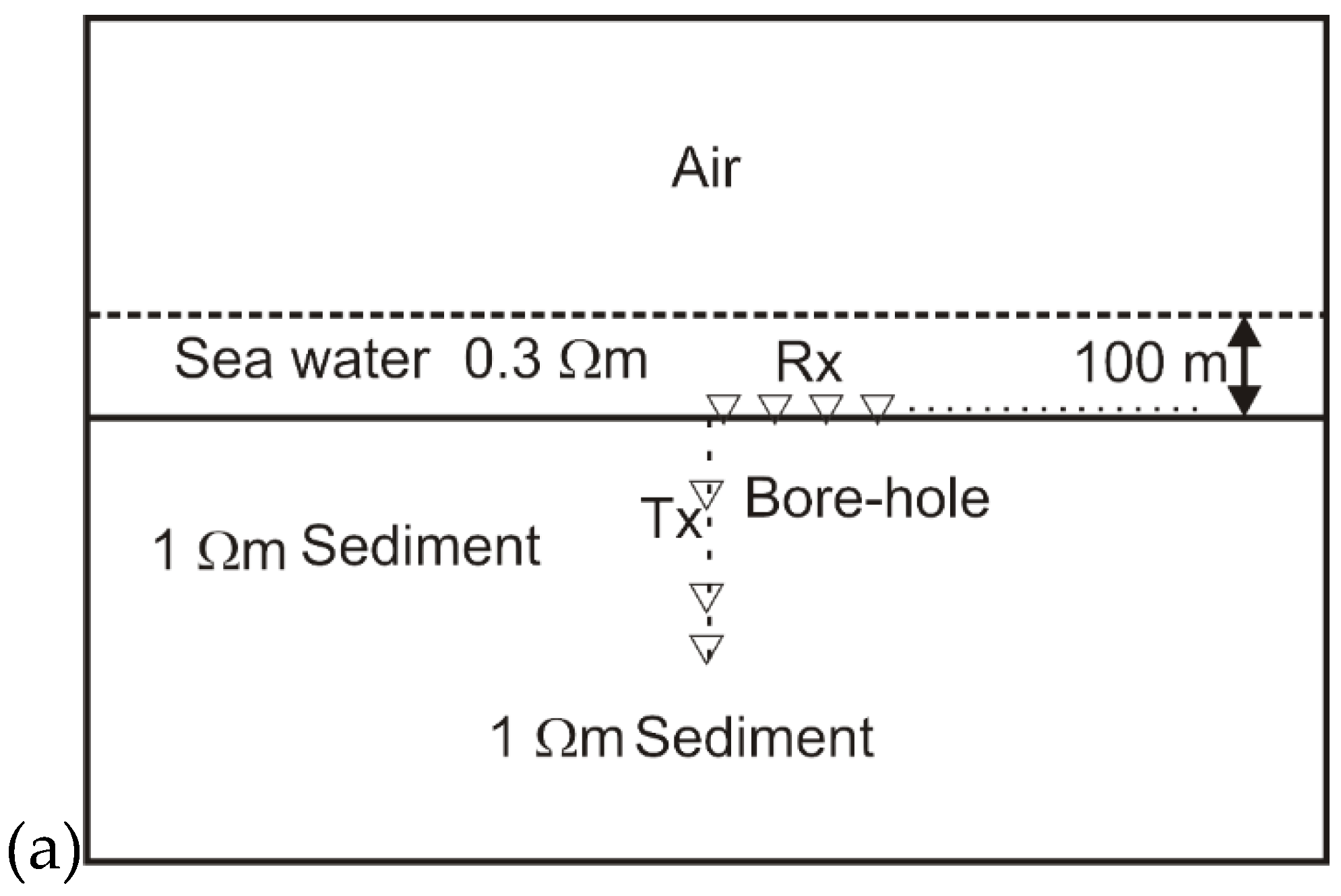
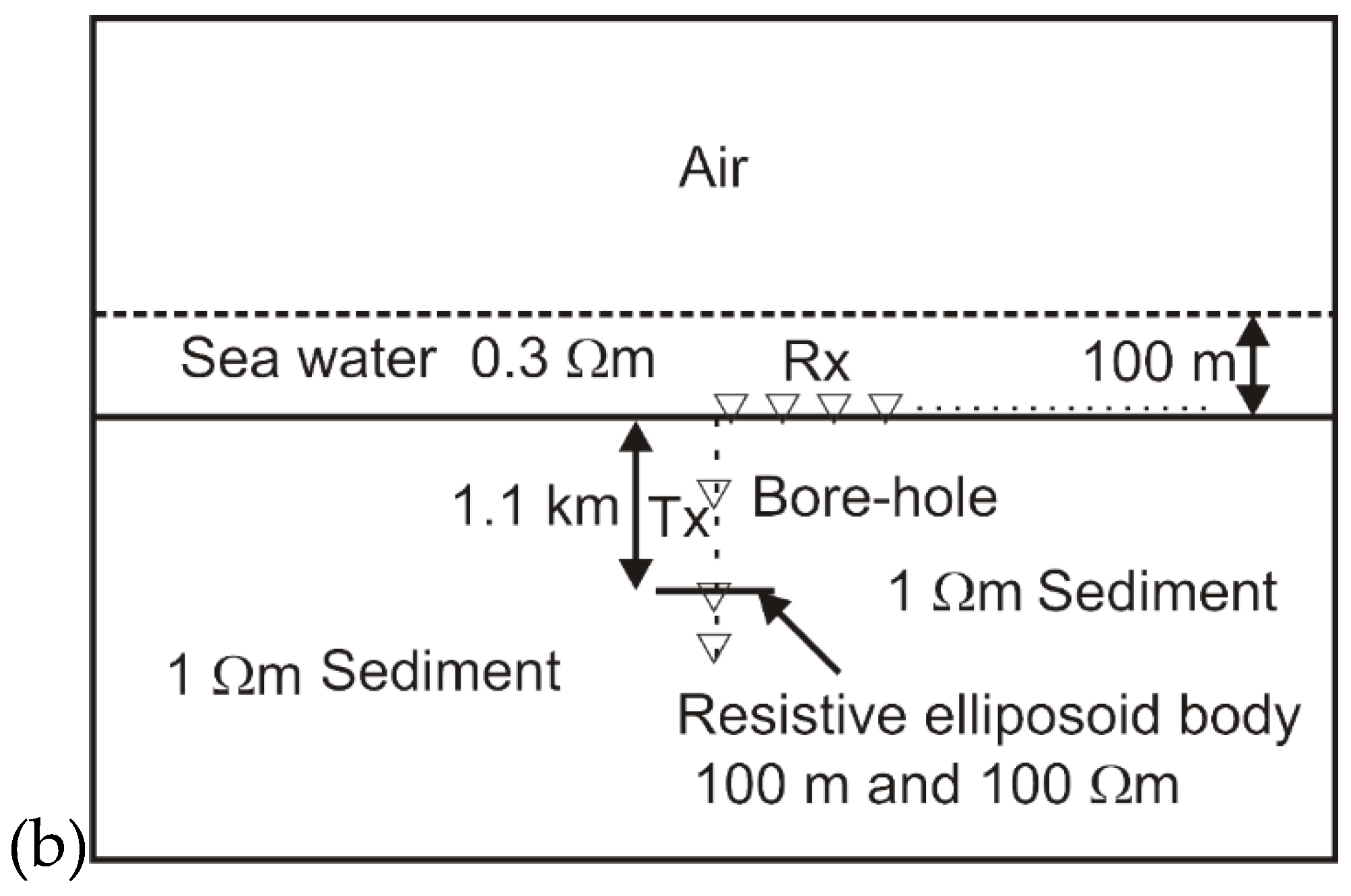
Figure 2.
Comparison of (a) amplitude normalised to unit source dipole moment and (b) phase of horizontal component of electric field at the seafloor as a function of horizontal source-receiver offset, as calculated for the half-space reference model and for varying source depths by the EH3D and 1D codes.
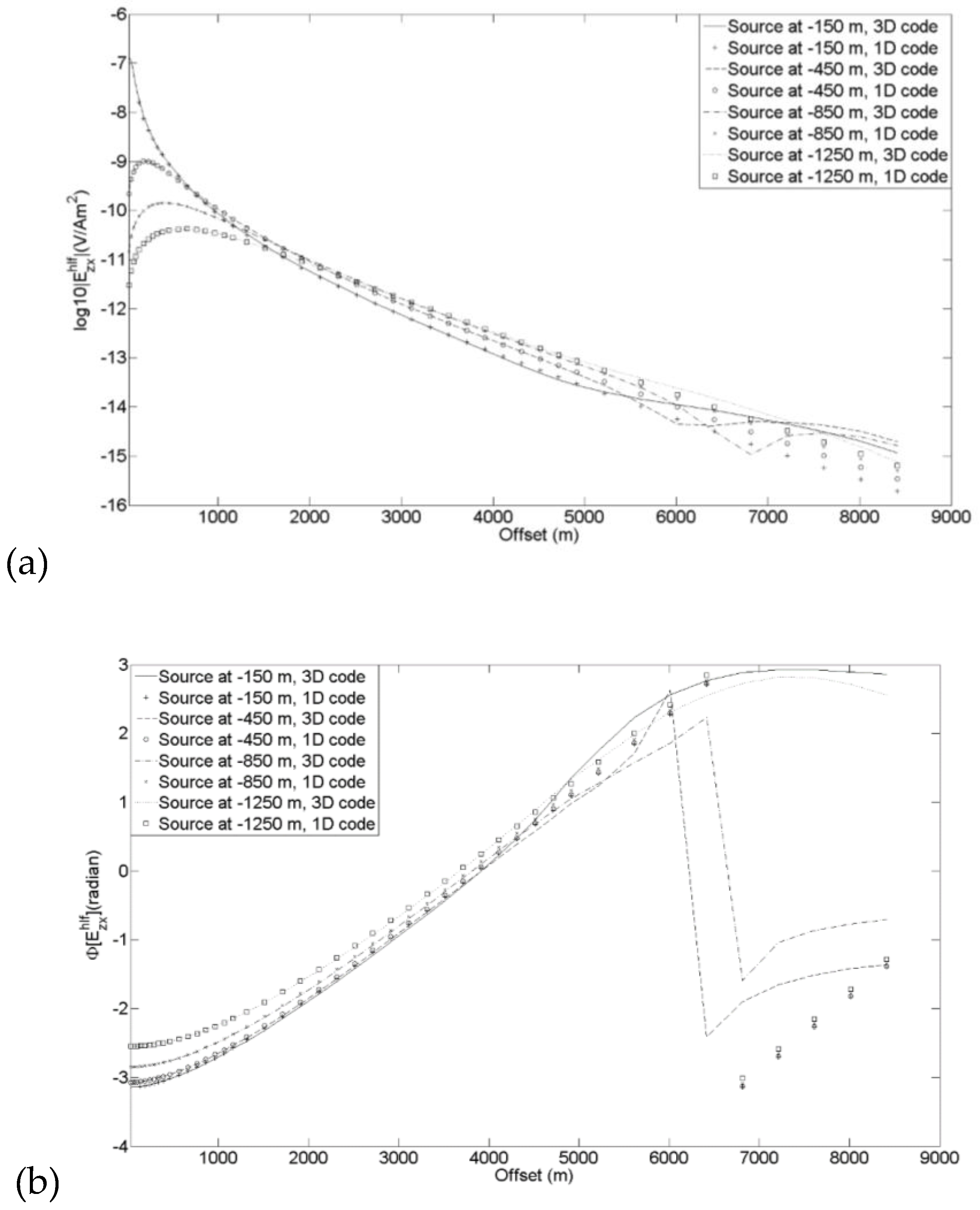
Figure 3.
Comparison of (a) amplitude normalised to unit source dipole moment and (b) phase of vertical component of electric field at the seafloor as a function of horizontal source-receiver offset, as calculated for the half-space reference model and for varying source depths by the EH3D and 1D codes.
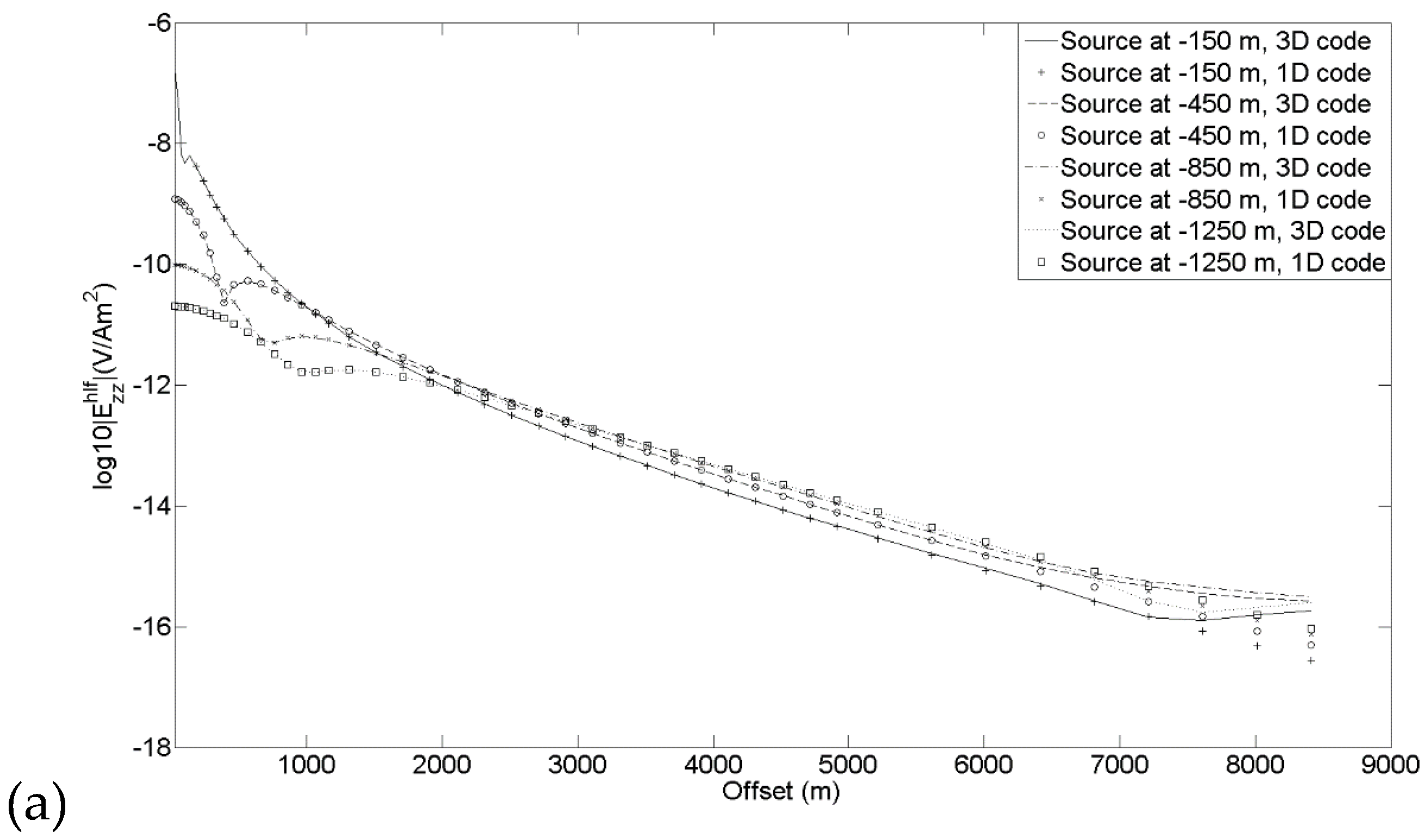
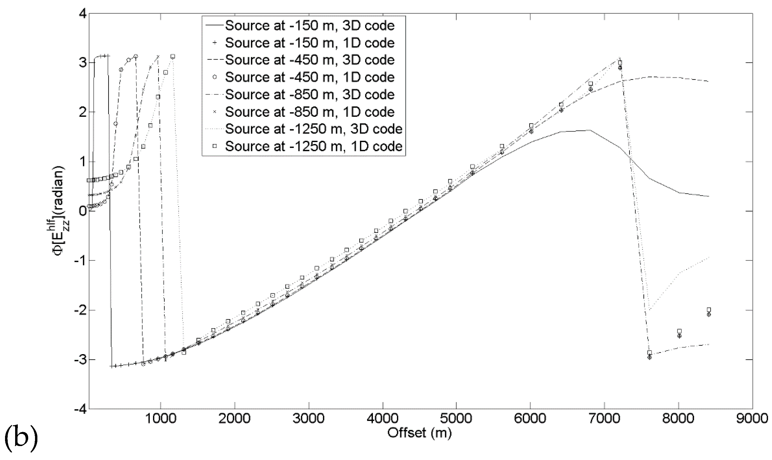
Figure 4.
The variation in electric field amplitudes normalised to unit source dipole moment for (a) horizontal and (b) vertical components of electric field as a function of horizontal offset, calculated at the seafloor for the centred resistive disk model at a range of frequencies. The transmitter is a 25 m long VED at a depth of 1.1 km below the seafloor. The water depth is 100 m. The locations of the disk and source are also plotted.
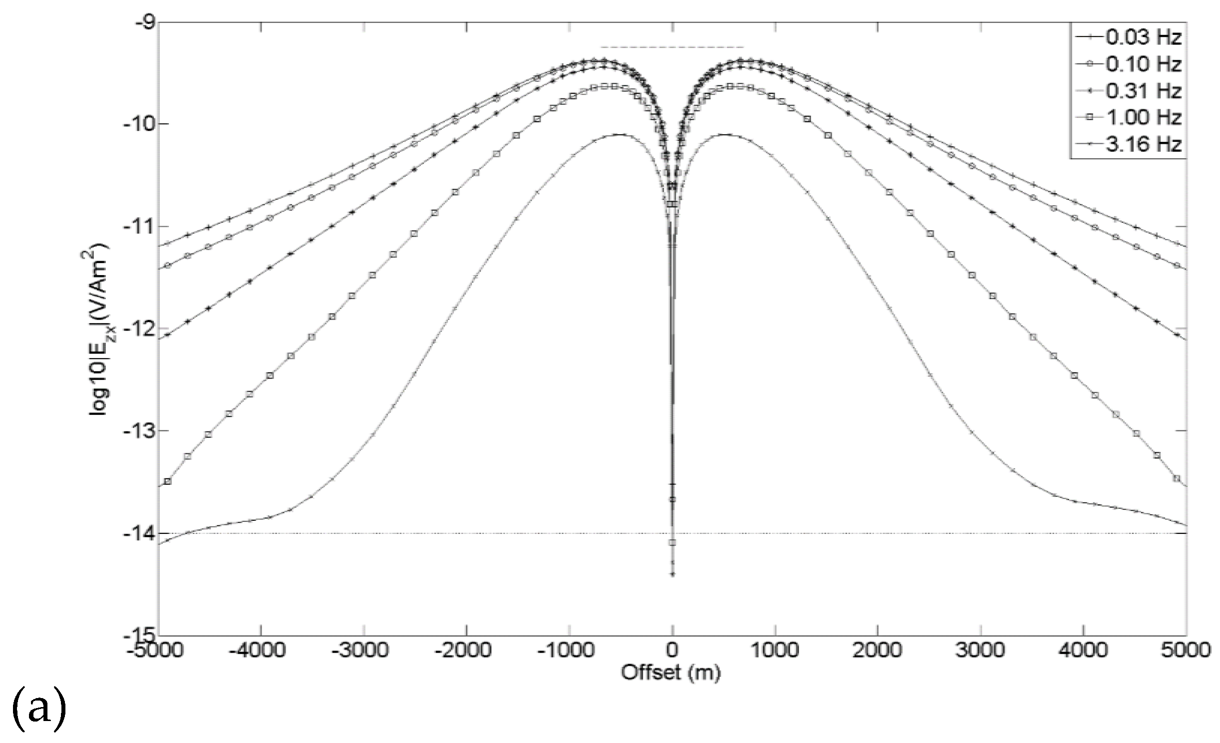
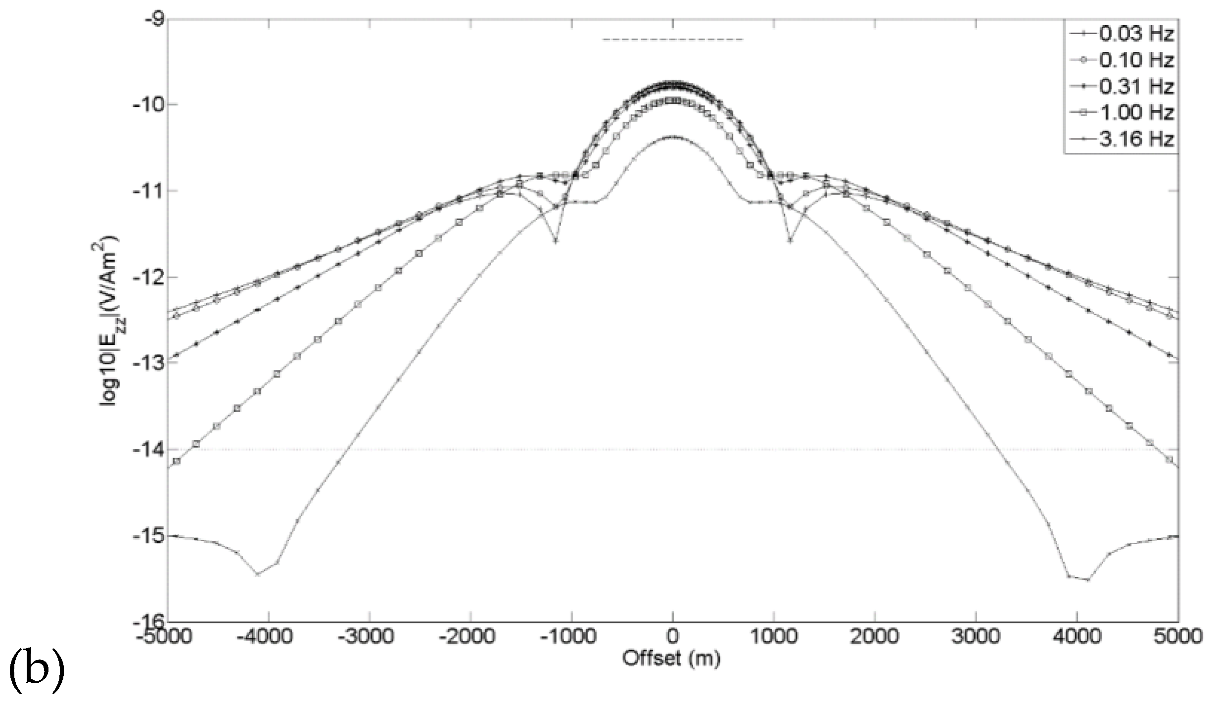
Figure 5.
Amplitude normalised to unit source dipole moment of (a) the horizontal and (b) the vertical components of electric field in the xz plane through the transmitter, for the half-space reference model.
Figure 5.
Amplitude normalised to unit source dipole moment of (a) the horizontal and (b) the vertical components of electric field in the xz plane through the transmitter, for the half-space reference model.
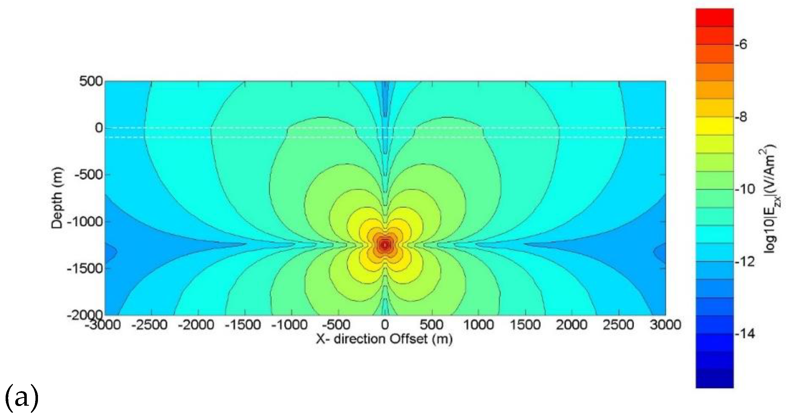
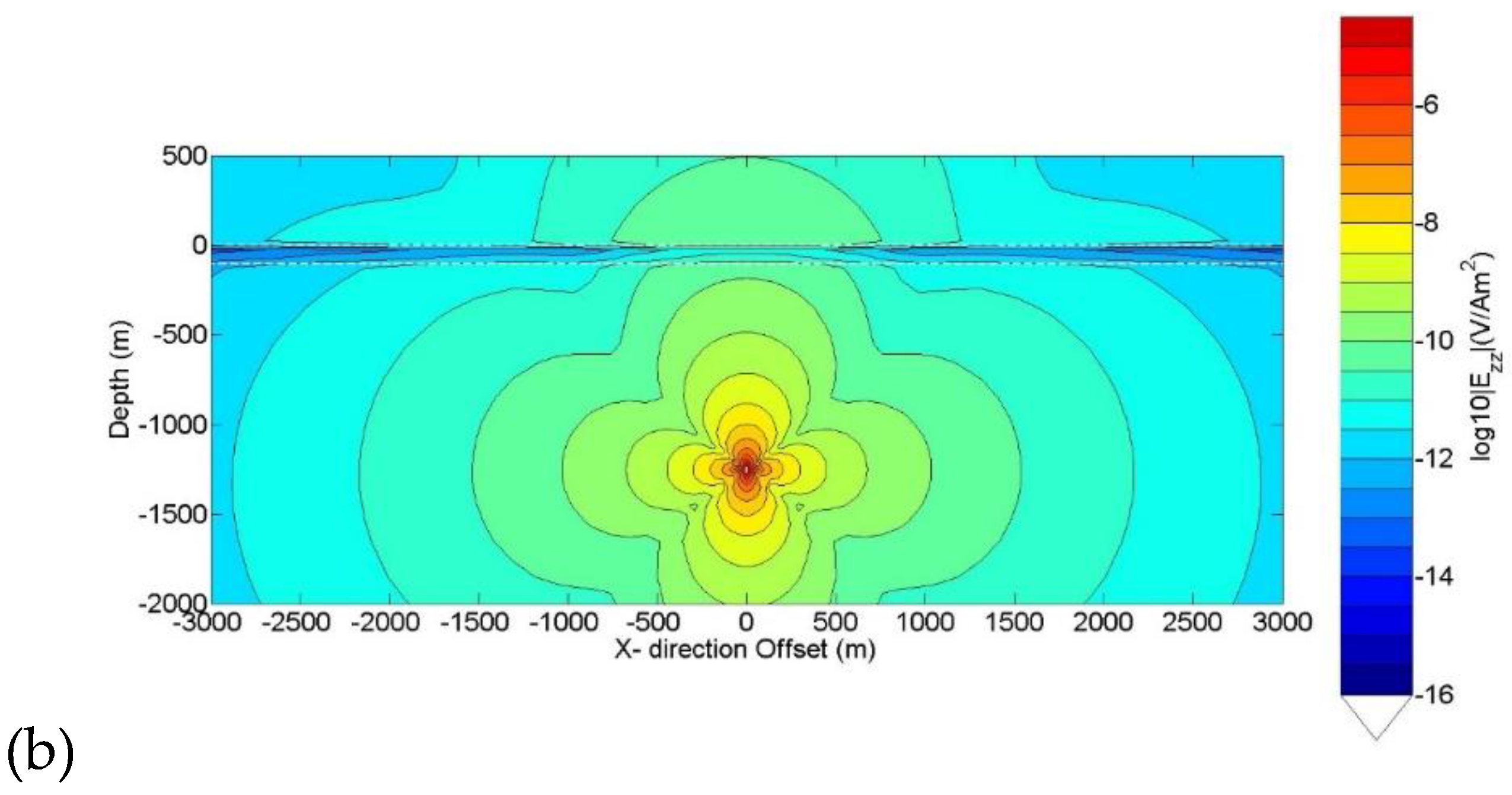
Figure 6.
Amplitude normalised to unit source dipole moment of (a) the horizontal and (b) the vertical components of electric field in the xz plane through the transmitter, for the centred resistive disk model. The locations of the disk and source are also plotted.
Figure 6.
Amplitude normalised to unit source dipole moment of (a) the horizontal and (b) the vertical components of electric field in the xz plane through the transmitter, for the centred resistive disk model. The locations of the disk and source are also plotted.
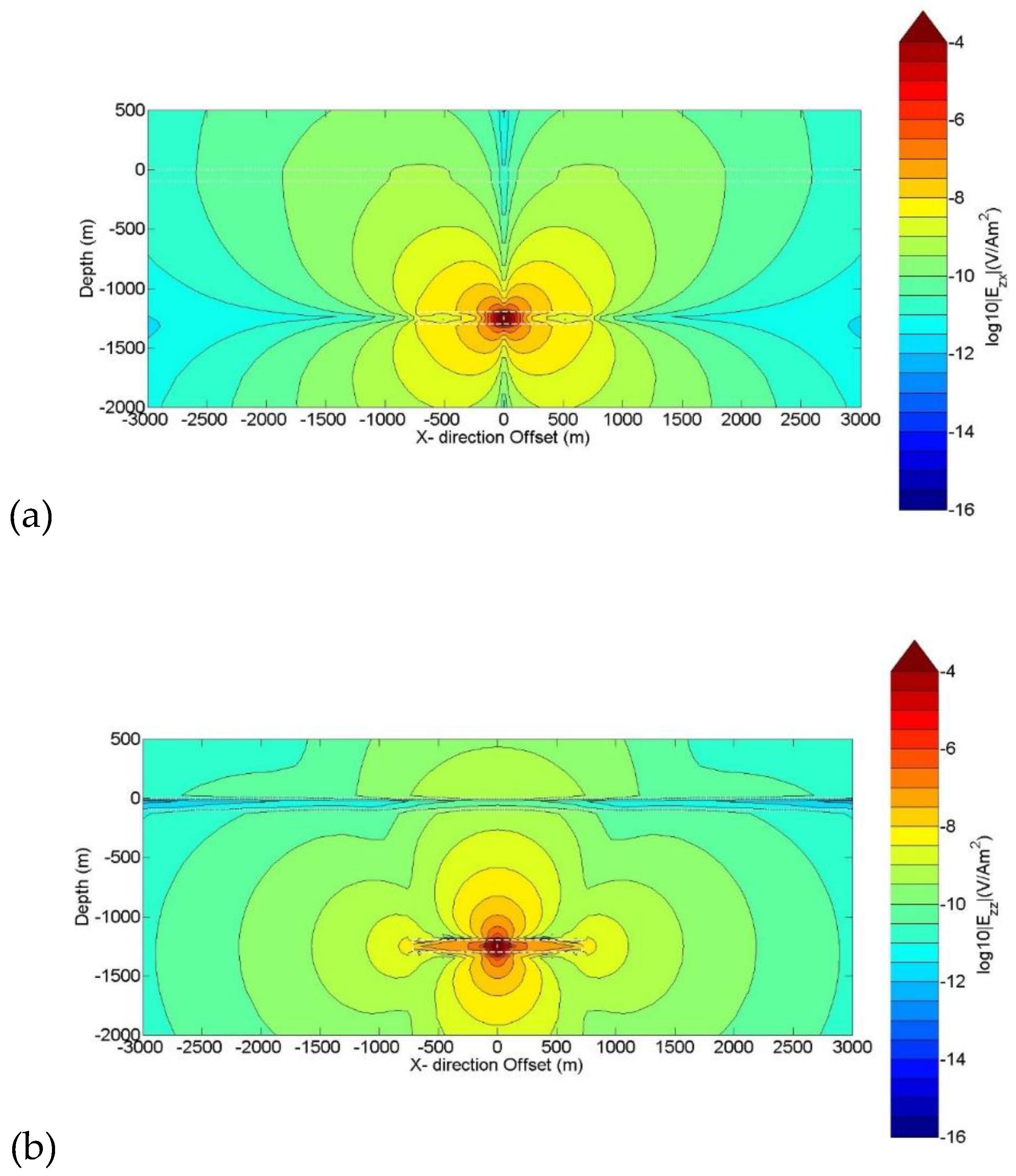
Figure 7.
Dimensionless amplitudes of (a) the horizontal and (b) the vertical components of electric field in the xz plane through the transmitter, for the half-space reference model.
Figure 7.
Dimensionless amplitudes of (a) the horizontal and (b) the vertical components of electric field in the xz plane through the transmitter, for the half-space reference model.
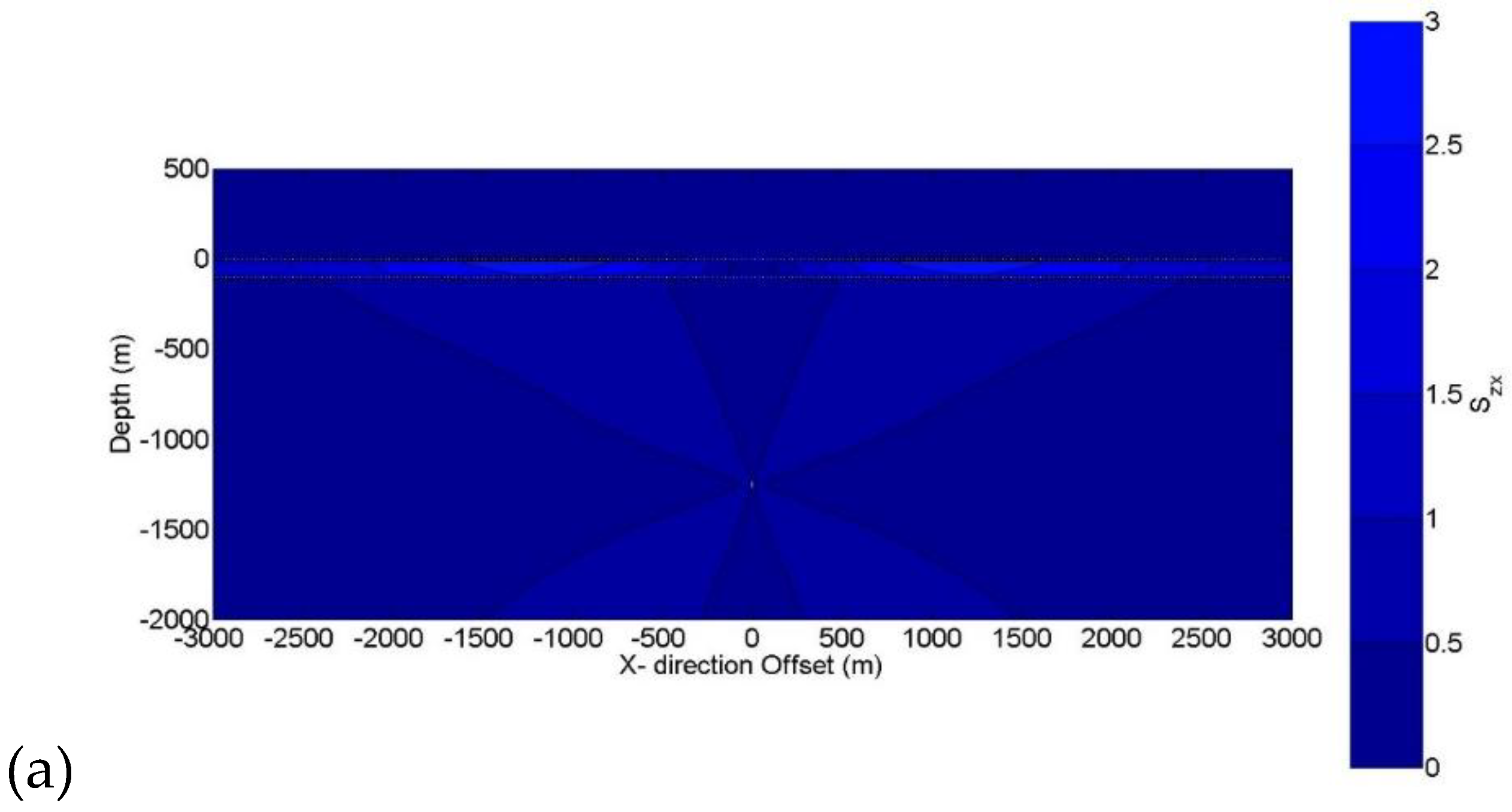
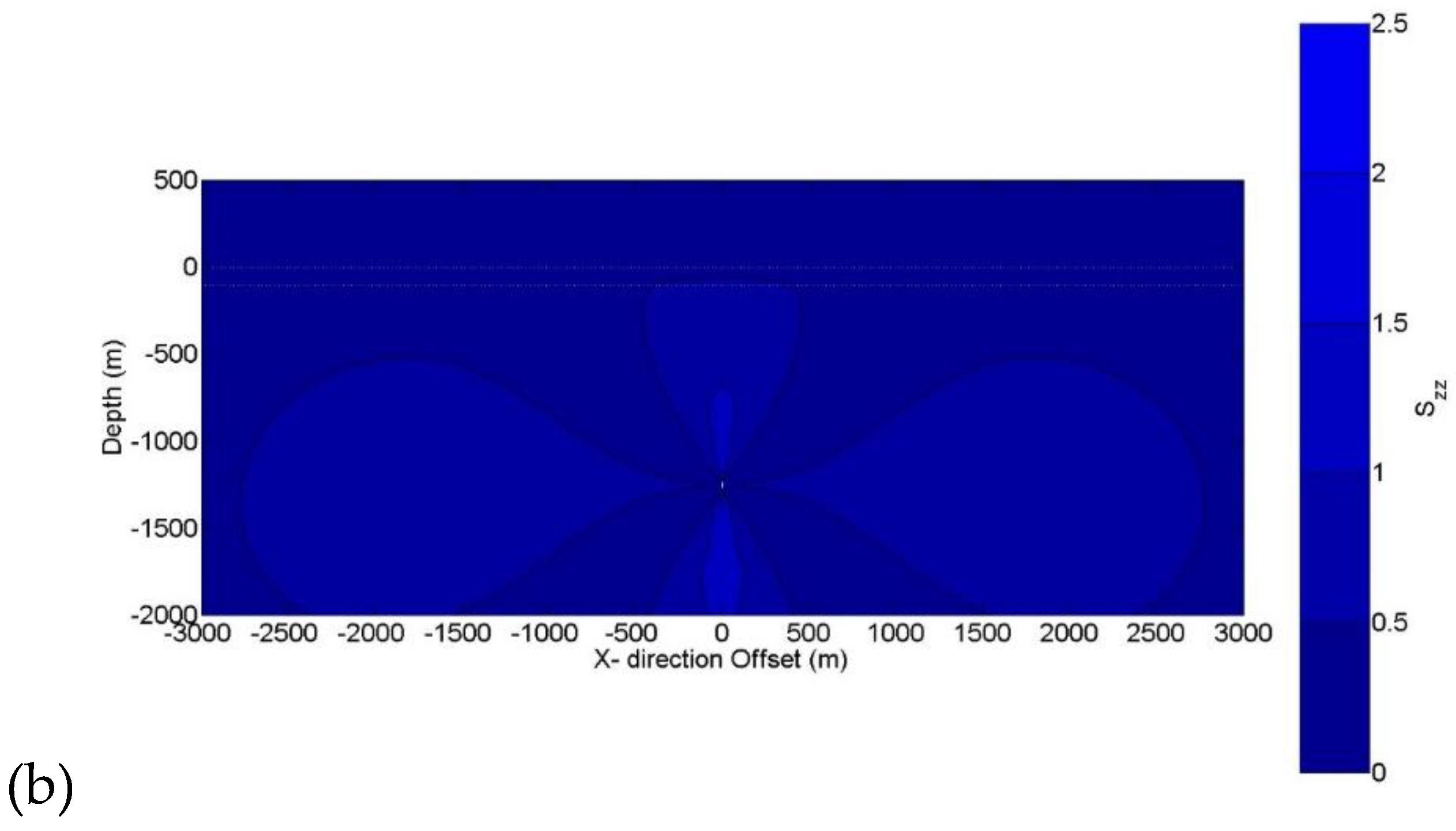
Figure 8.
Dimensionless amplitudes of (a) the horizontal and (b) the vertical components of electric field in the xz plane through the transmitter, for the thin resistive layer model. The locations of the disk and source are also plotted.
Figure 8.
Dimensionless amplitudes of (a) the horizontal and (b) the vertical components of electric field in the xz plane through the transmitter, for the thin resistive layer model. The locations of the disk and source are also plotted.
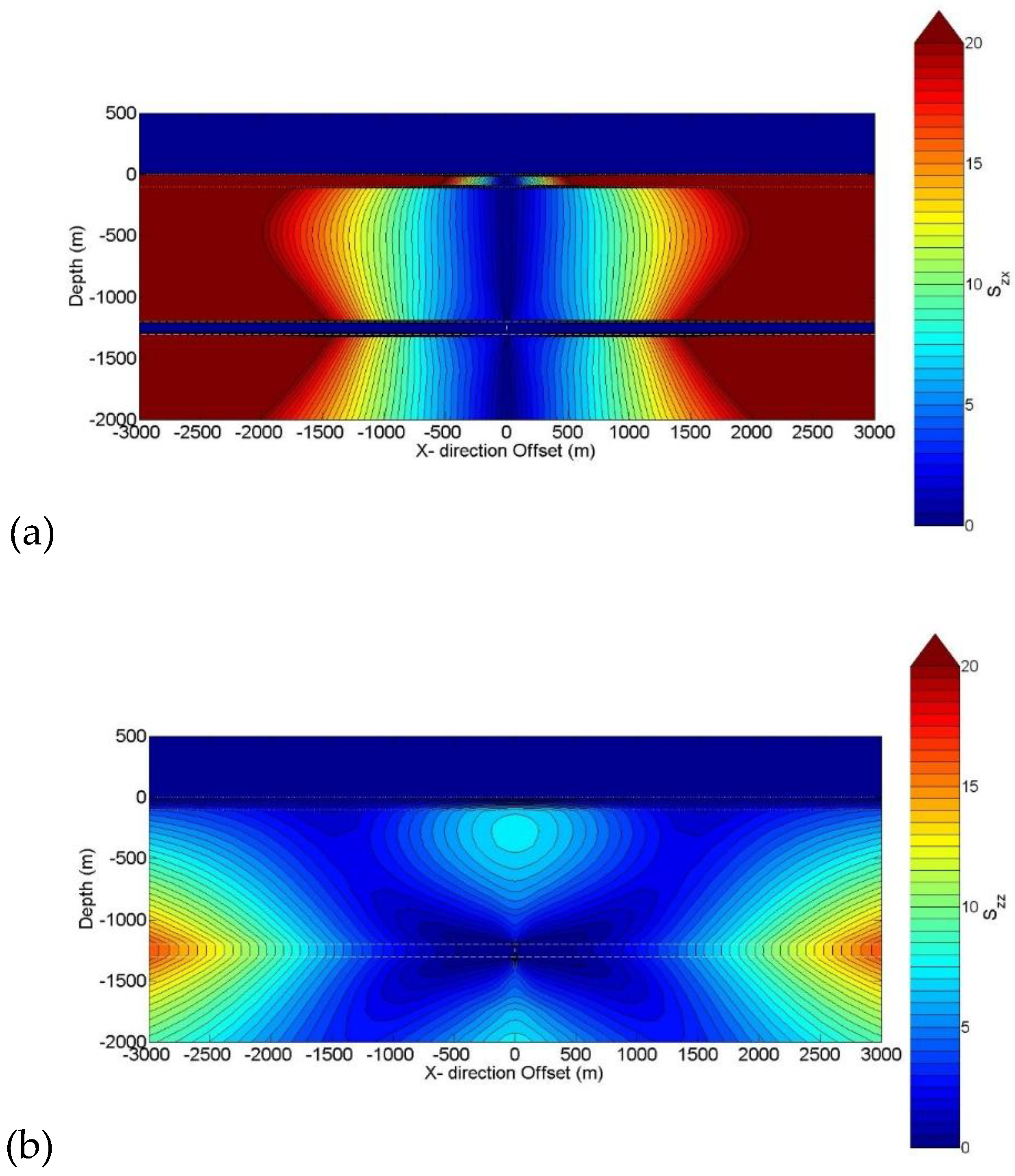
Figure 9.
Dimensionless amplitudes of (a) the horizontal and (b) the vertical components of electric field in the xz plane through the transmitter, for the centred resistive disk model. The locations of the disk and source are also plotted.
Figure 9.
Dimensionless amplitudes of (a) the horizontal and (b) the vertical components of electric field in the xz plane through the transmitter, for the centred resistive disk model. The locations of the disk and source are also plotted.
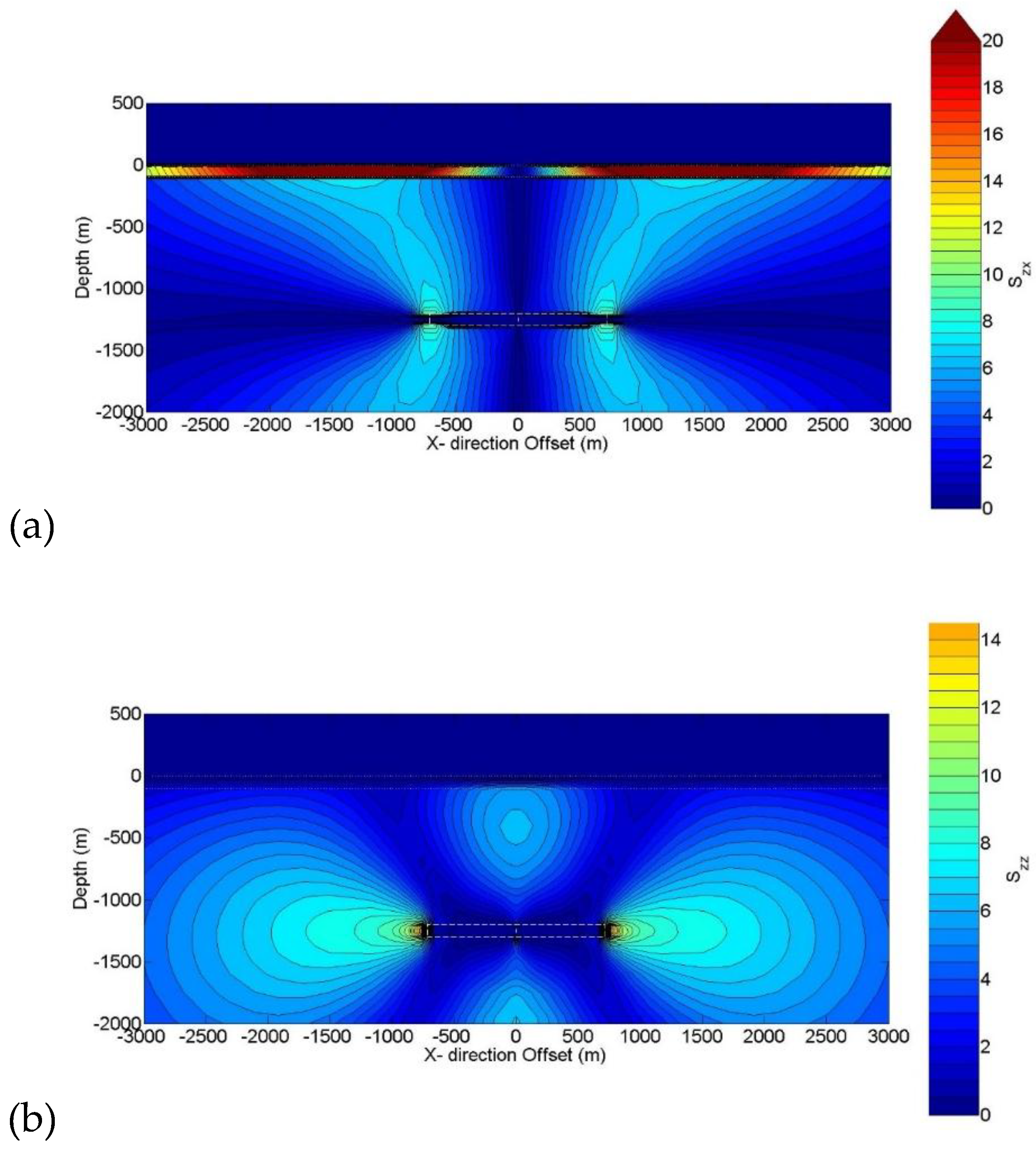
Figure 10.
Dimensionless amplitudes of (a) the horizontal and (b) the vertical components of electric field in the xz plane through the transmitter, for the just inside model. The locations of the disk and source are also plotted.
Figure 10.
Dimensionless amplitudes of (a) the horizontal and (b) the vertical components of electric field in the xz plane through the transmitter, for the just inside model. The locations of the disk and source are also plotted.
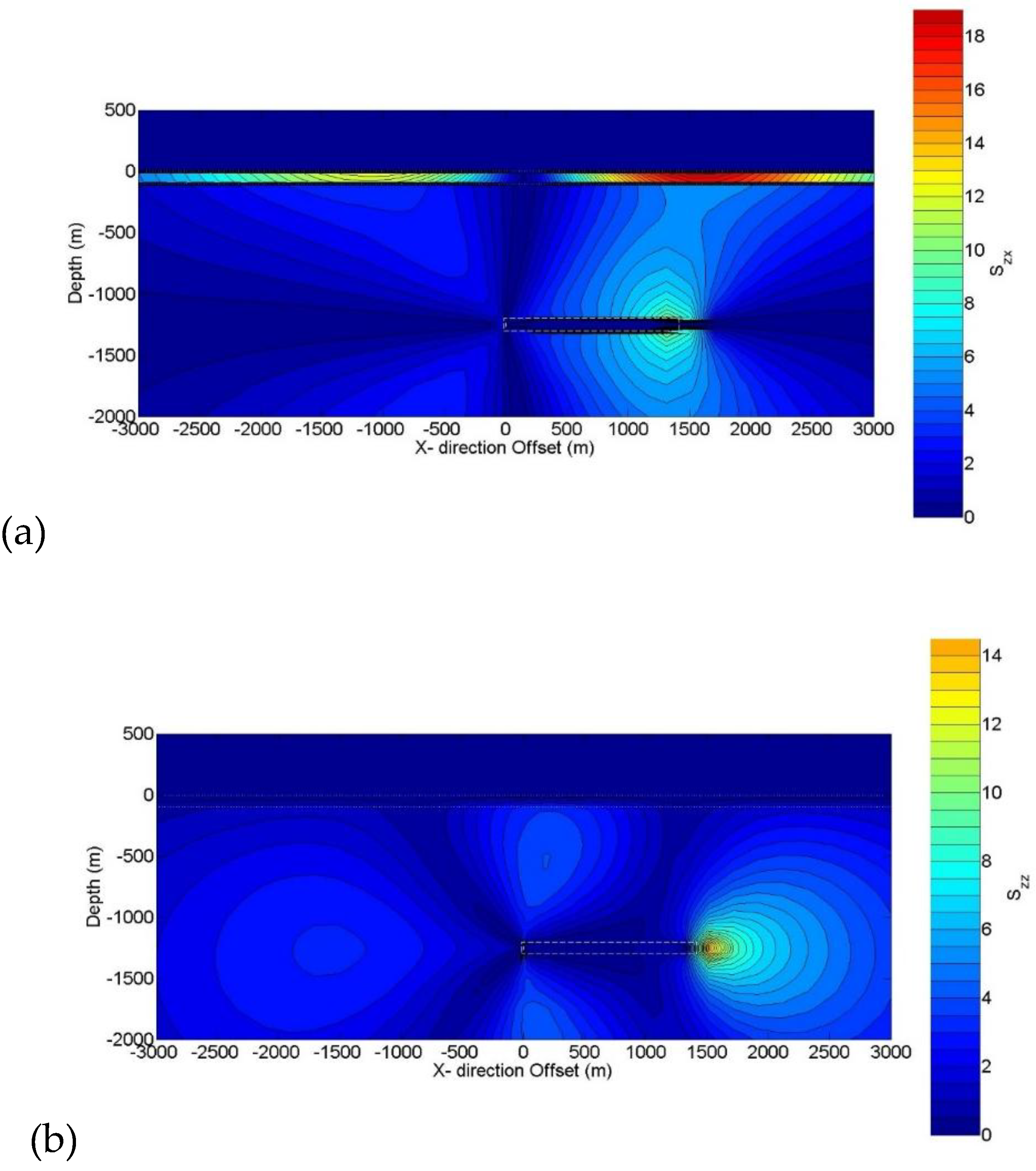
Figure 11.
Dimensionless amplitudes of (a) the horizontal and (b) the vertical components of electric field in the xz plane through the transmitter, for the just outside model. The locations of the disk and source are also plotted.
Figure 11.
Dimensionless amplitudes of (a) the horizontal and (b) the vertical components of electric field in the xz plane through the transmitter, for the just outside model. The locations of the disk and source are also plotted.
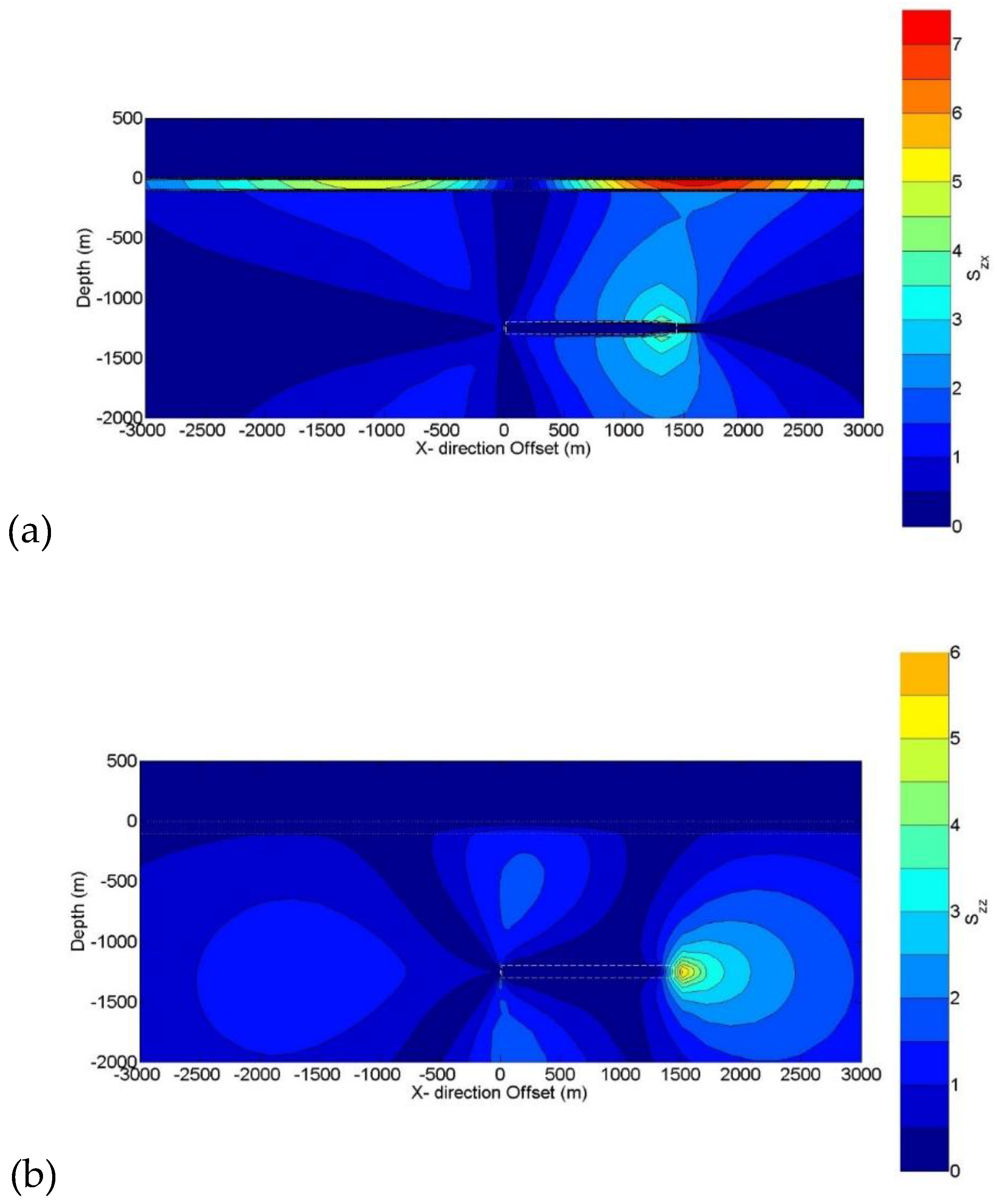
Figure 12.
Dimensionless amplitudes of (a) the horizontal and (b) the vertical components of electric field at the seafloor for various models. The locations of the disk are also plotted, and they only vary in horizontal direction not in vertical direction.
Figure 12.
Dimensionless amplitudes of (a) the horizontal and (b) the vertical components of electric field at the seafloor for various models. The locations of the disk are also plotted, and they only vary in horizontal direction not in vertical direction.
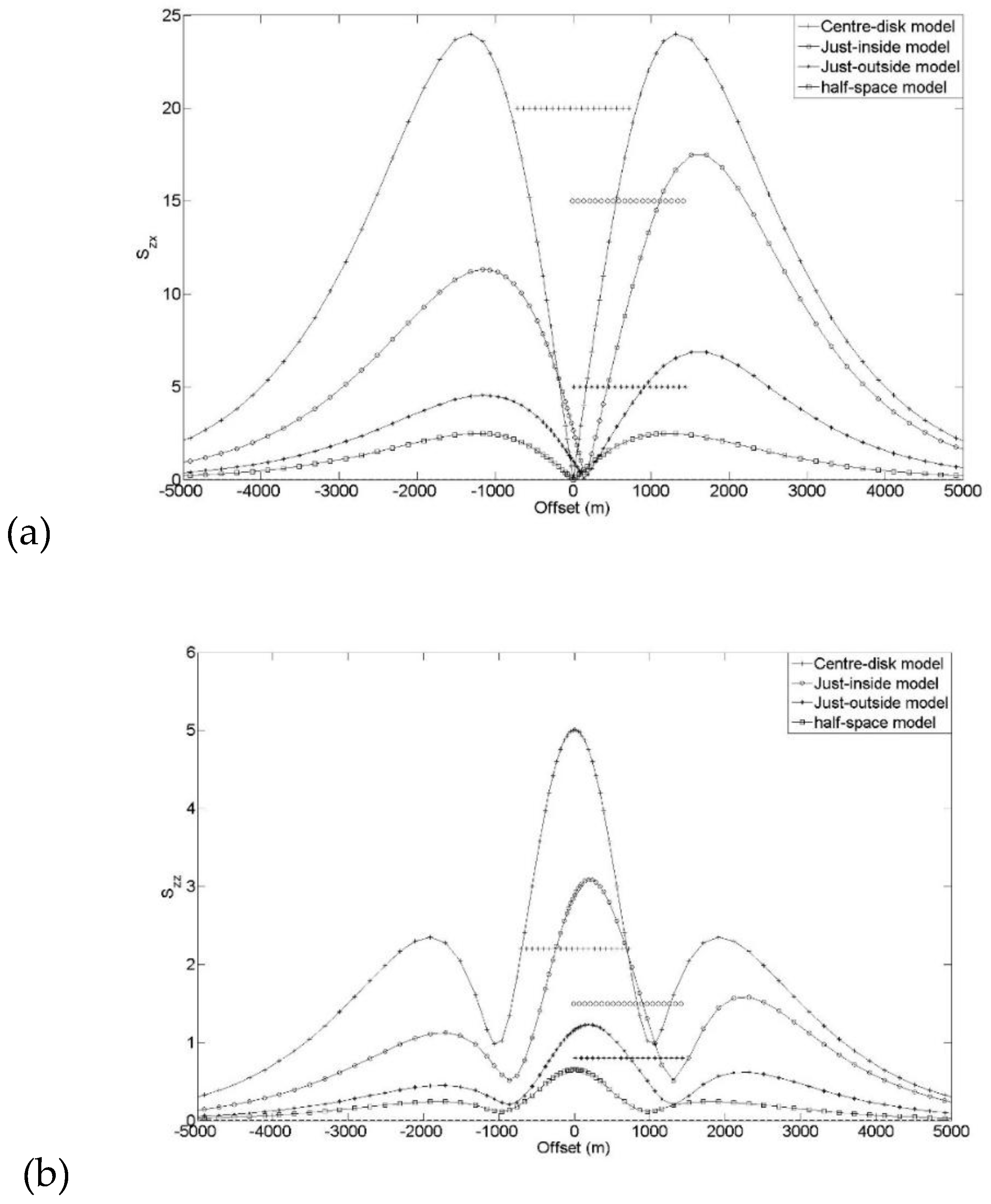
Figure 13.
Contour plot of a plan view of horizontal dimensionless amplitude response at the seafloor for the just outside model. (a) Sz,rad component. (b) The null-coupled Sz,tan component. The locations of the disk and source are also plotted.
Figure 13.
Contour plot of a plan view of horizontal dimensionless amplitude response at the seafloor for the just outside model. (a) Sz,rad component. (b) The null-coupled Sz,tan component. The locations of the disk and source are also plotted.
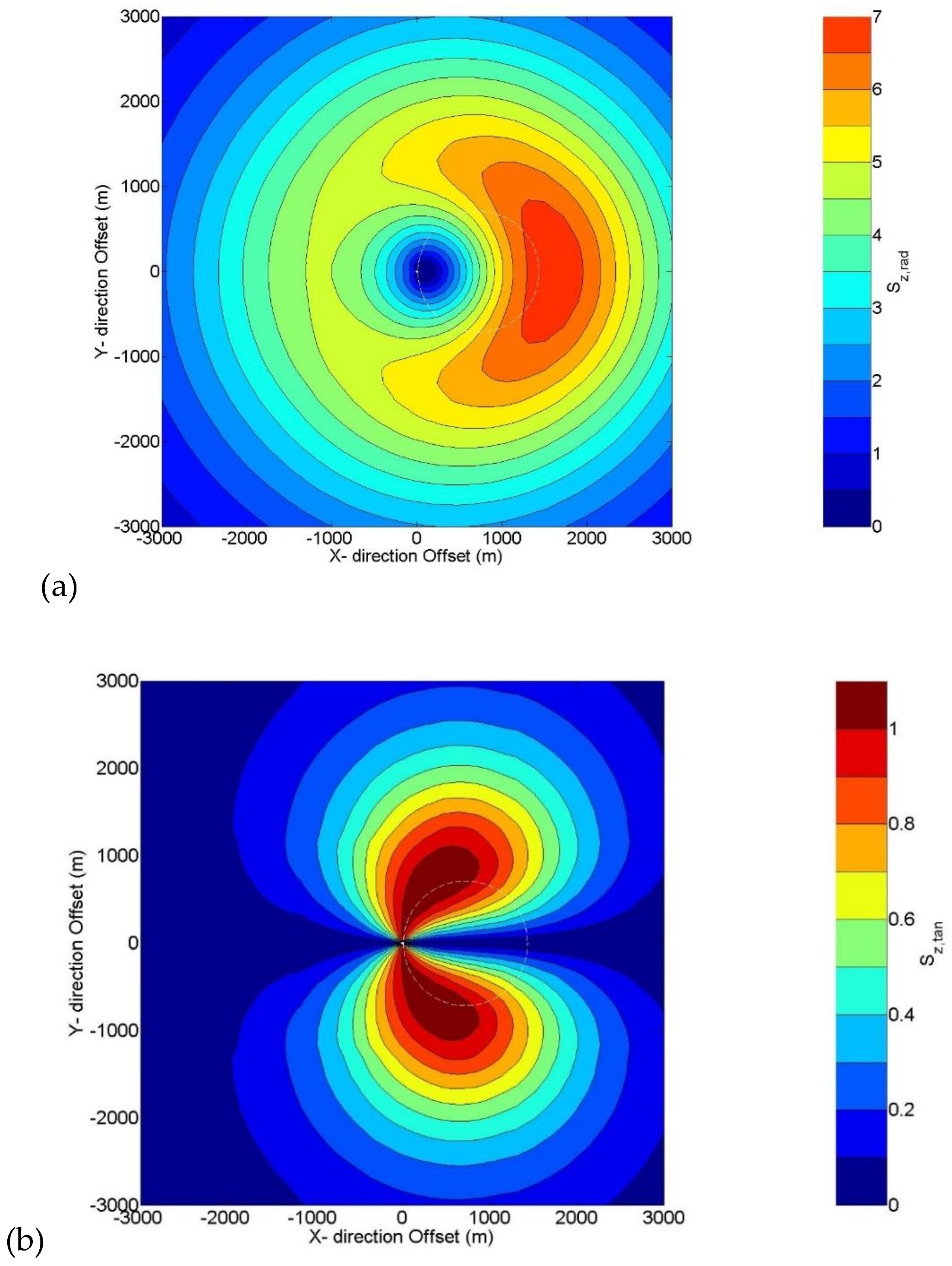
Figure 14.
Dimensionless amplitudes of (a) the horizontal and (b) the vertical components of electric field at the seafloor for variants of the resistive disk model with a range of horizontal offsets of the borehole from the nearest edge of the target. The locations of source and target are also plotted.
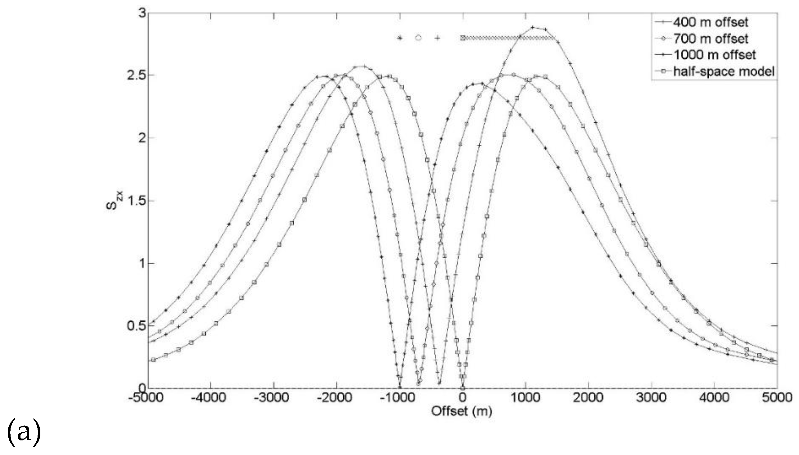
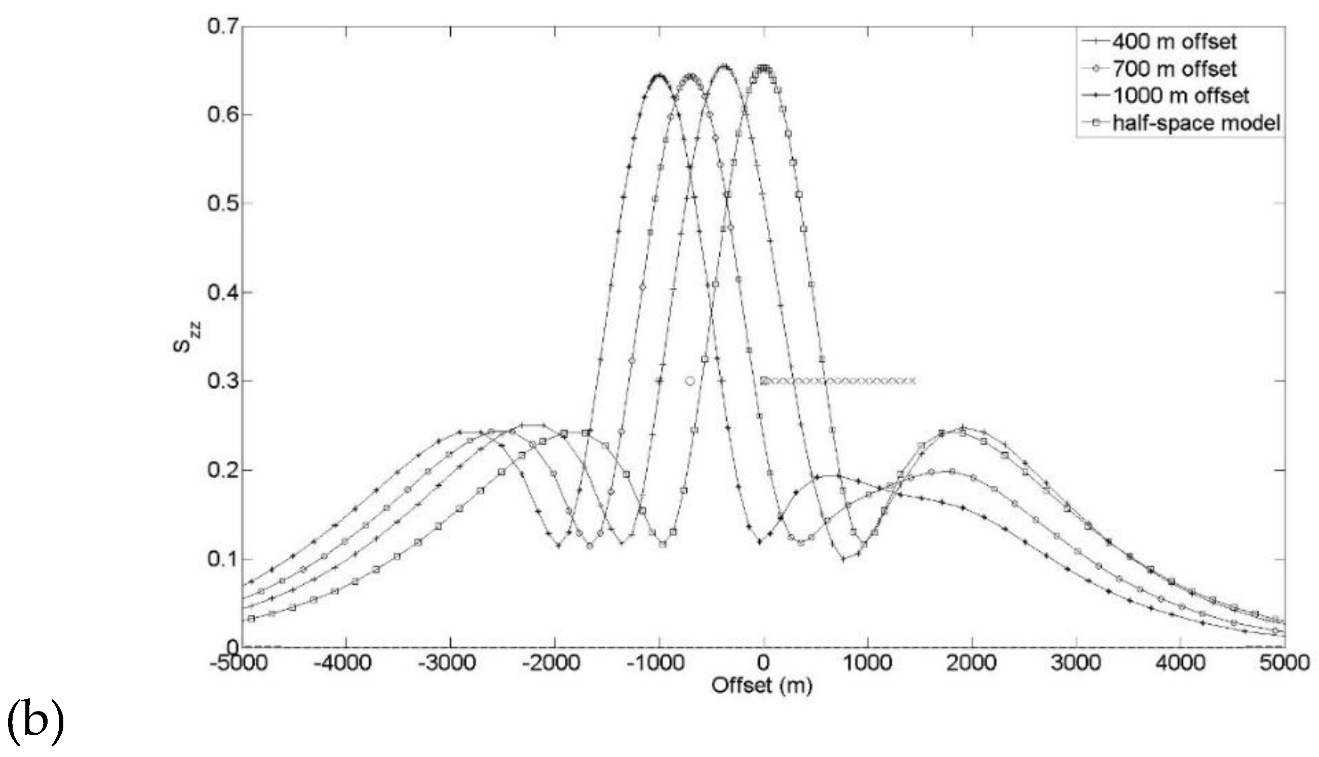
Figure 15.
Percentage difference between the modelled response and that of the half-space reference model of (a) the horizontal and (b) the vertical components of electric field at the seafloor for variants of the resistive disk model with a range of horizontal offsets of the borehole from the nearest edge of the target, presented as the. The locations of targets are also plotted.
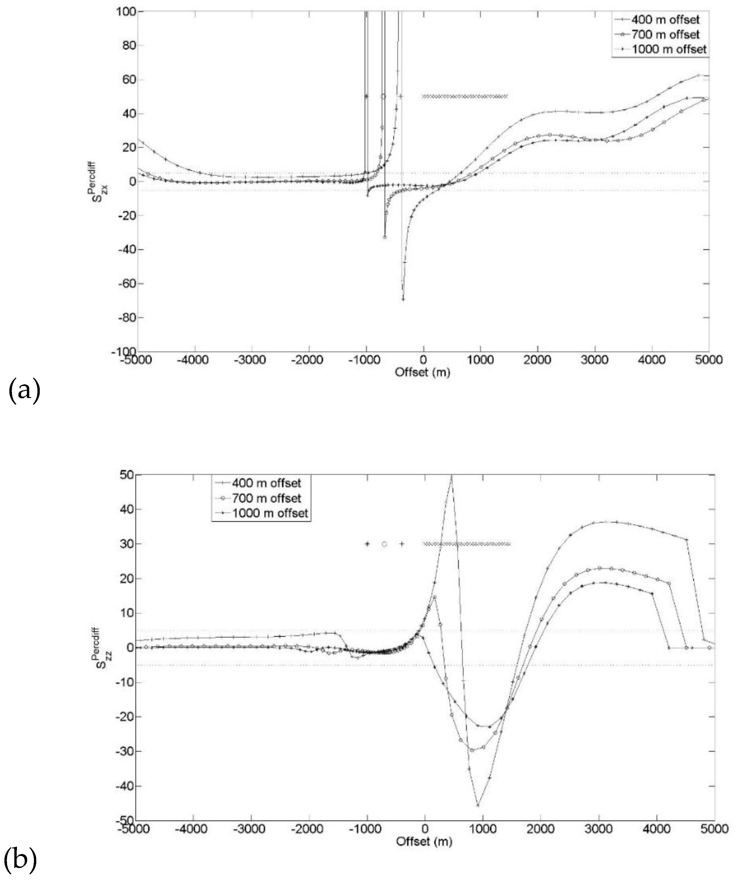
Figure 16.
Dimensionless amplitudes of (a) the horizontal and (b) the vertical components of electric field at the seafloor for the stacked reservoir model for various combinations of resistive targets and transmitter depths. The locations of targets are also plotted.
Figure 16.
Dimensionless amplitudes of (a) the horizontal and (b) the vertical components of electric field at the seafloor for the stacked reservoir model for various combinations of resistive targets and transmitter depths. The locations of targets are also plotted.
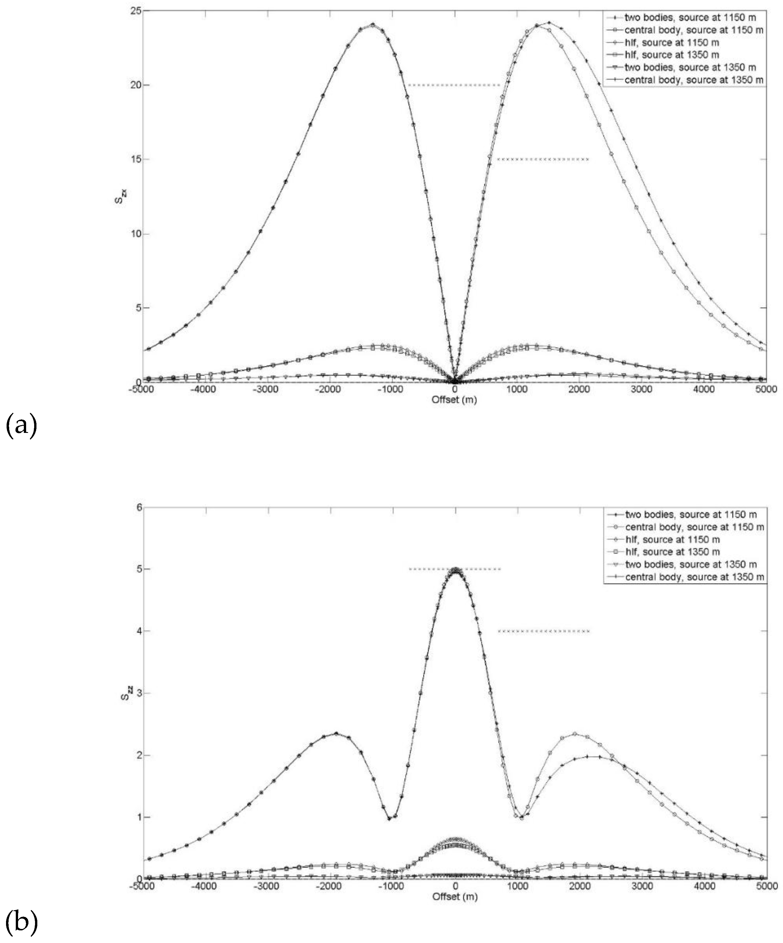
Figure 17.
Percentage differences of dimensionless amplitudes between the modelled response and that of the corresponding centred resistive disk model of (a) the horizontal and (b) the vertical components of the electric field at the seafloor for the stacked reservoir model for two transmitter depths. The locations of targets are also plotted.
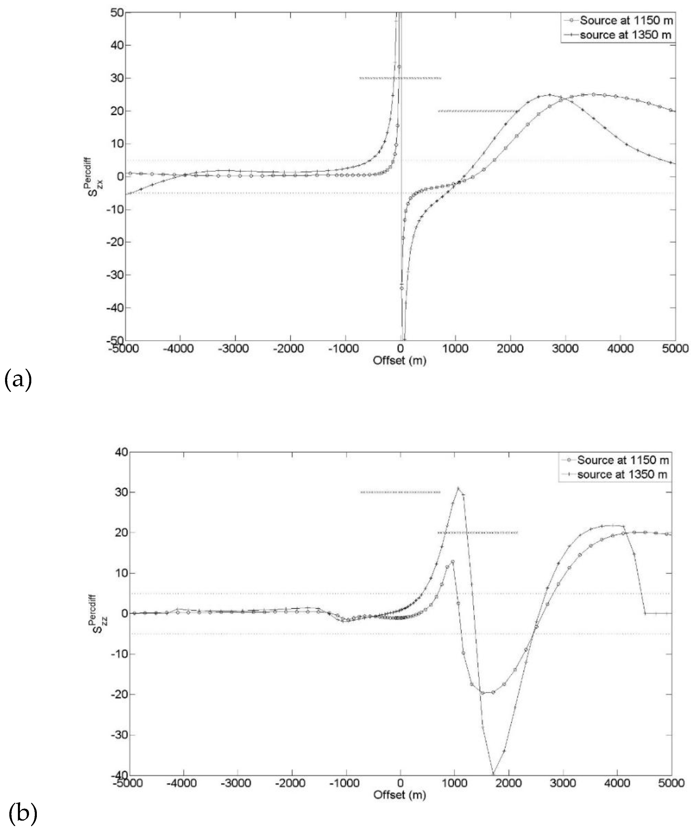
Figure 18.
Dimensionless amplitudes of (a) the horizontal and (b) the vertical components of electric field at the seafloor for variants of the resistive disk model for a range of horizontal offsets of the target, and for a target depth of 3 km. The locations of source and target are also plotted.
Figure 18.
Dimensionless amplitudes of (a) the horizontal and (b) the vertical components of electric field at the seafloor for variants of the resistive disk model for a range of horizontal offsets of the target, and for a target depth of 3 km. The locations of source and target are also plotted.
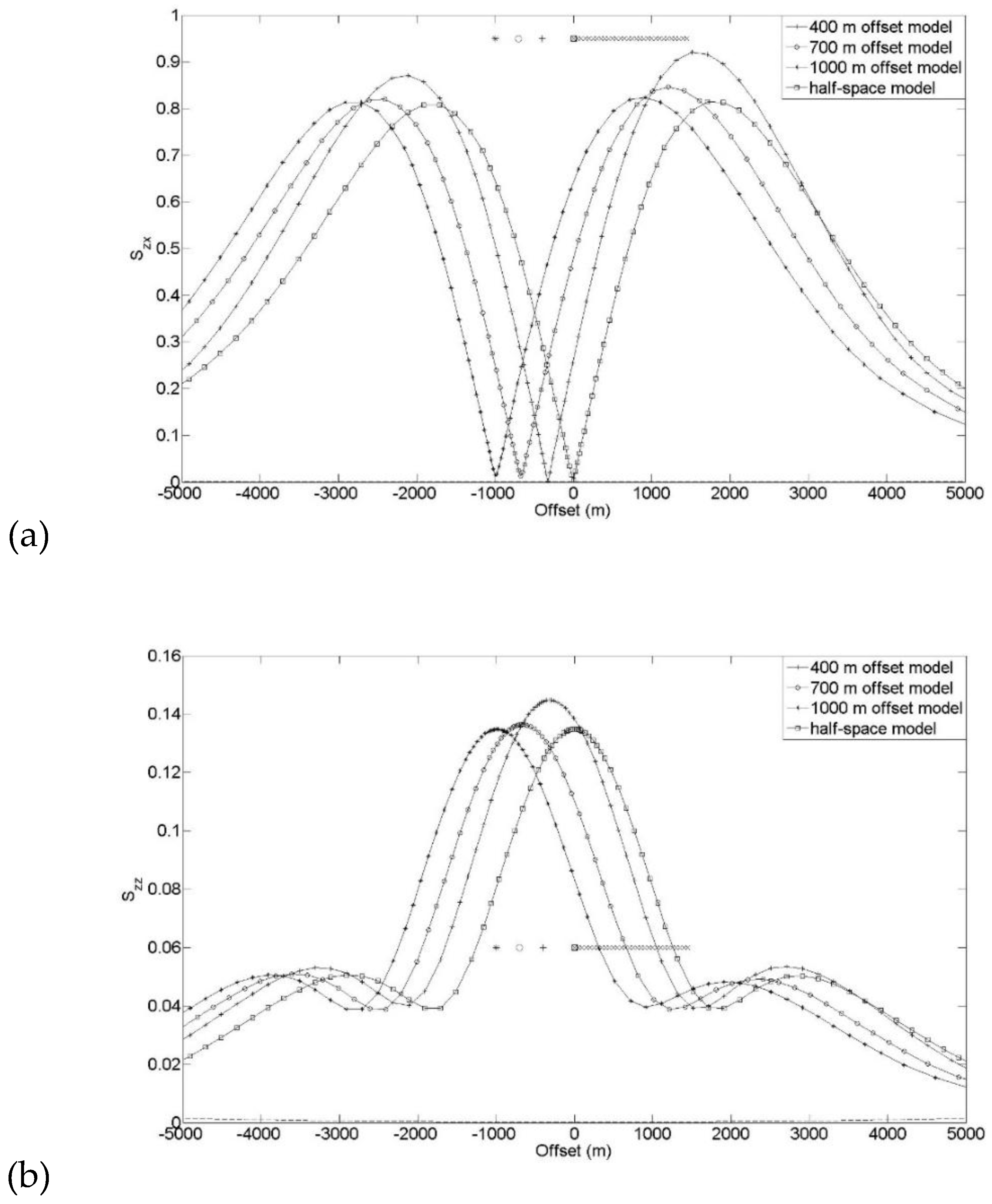
Figure 19.
Percentage differences between the modelled response and that of the half-space reference model of (a) the horizontal and (b) the vertical components of electric field at the seafloor for variants of the resistive disk model for a range of horizontal offsets of the target, and for a target depth of 3 km. The locations of source and target are also plotted.
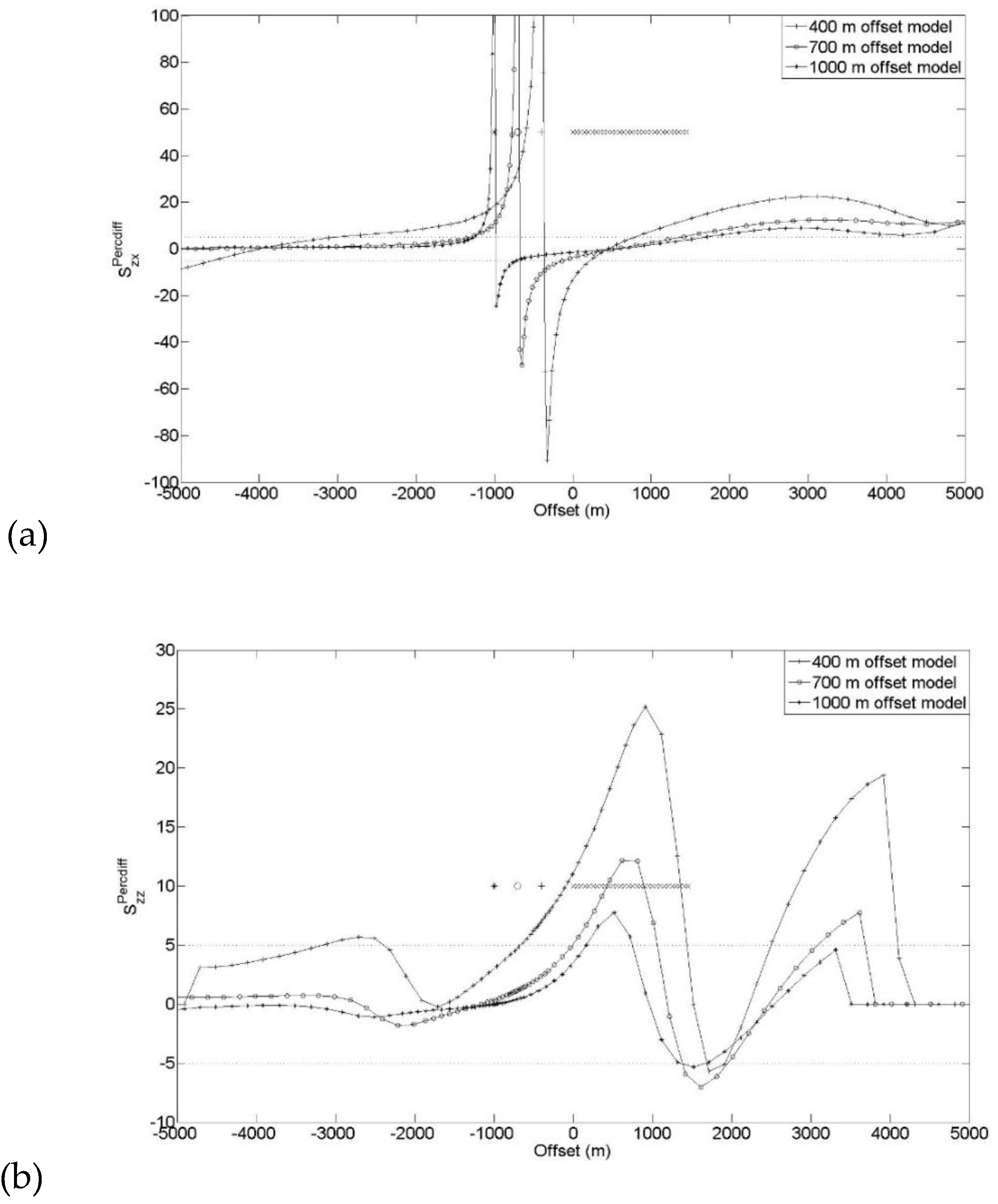
Figure 20.
Dimensionless amplitudes of (a) the horizontal and (b) the vertical components of electric field at the seafloor for variants of the stacked reservoir model for various combinations of resistive targets and transmitter depths, and in which the depths of the two target structures are 3.0 and 3.2 km respectively. The locations of targets are also plotted.
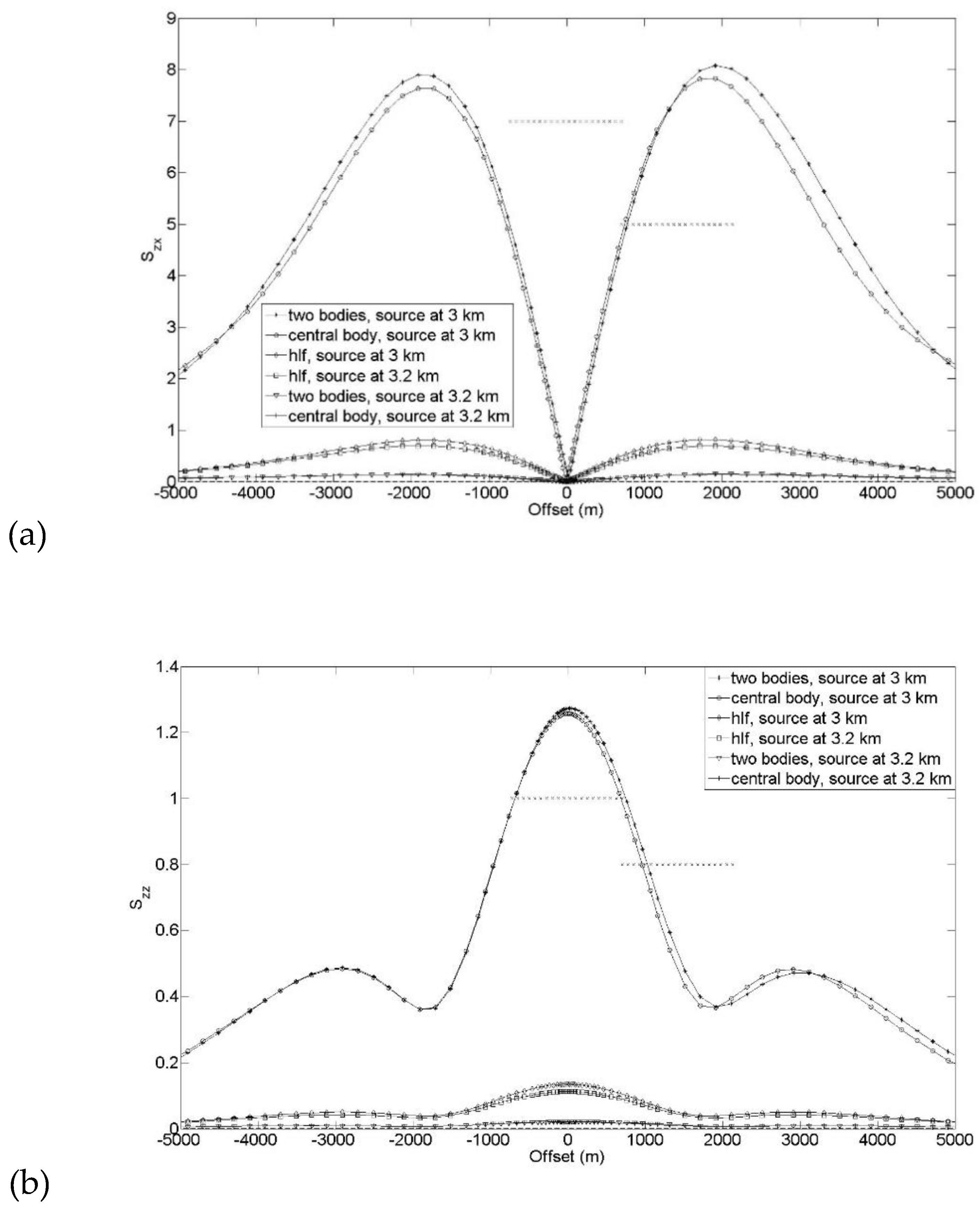
Figure 21.
Percentage differences between the modelled response and that of the corresponding centred resistive disk model of (a) the horizontal and (b) the vertical components of electric field at the seafloor for variants of the stacked reservoir model for two transmitter depths, in which the depths of the two target structures are 3.0 and 3.2 km respectively. The locations of targets are also plotted.
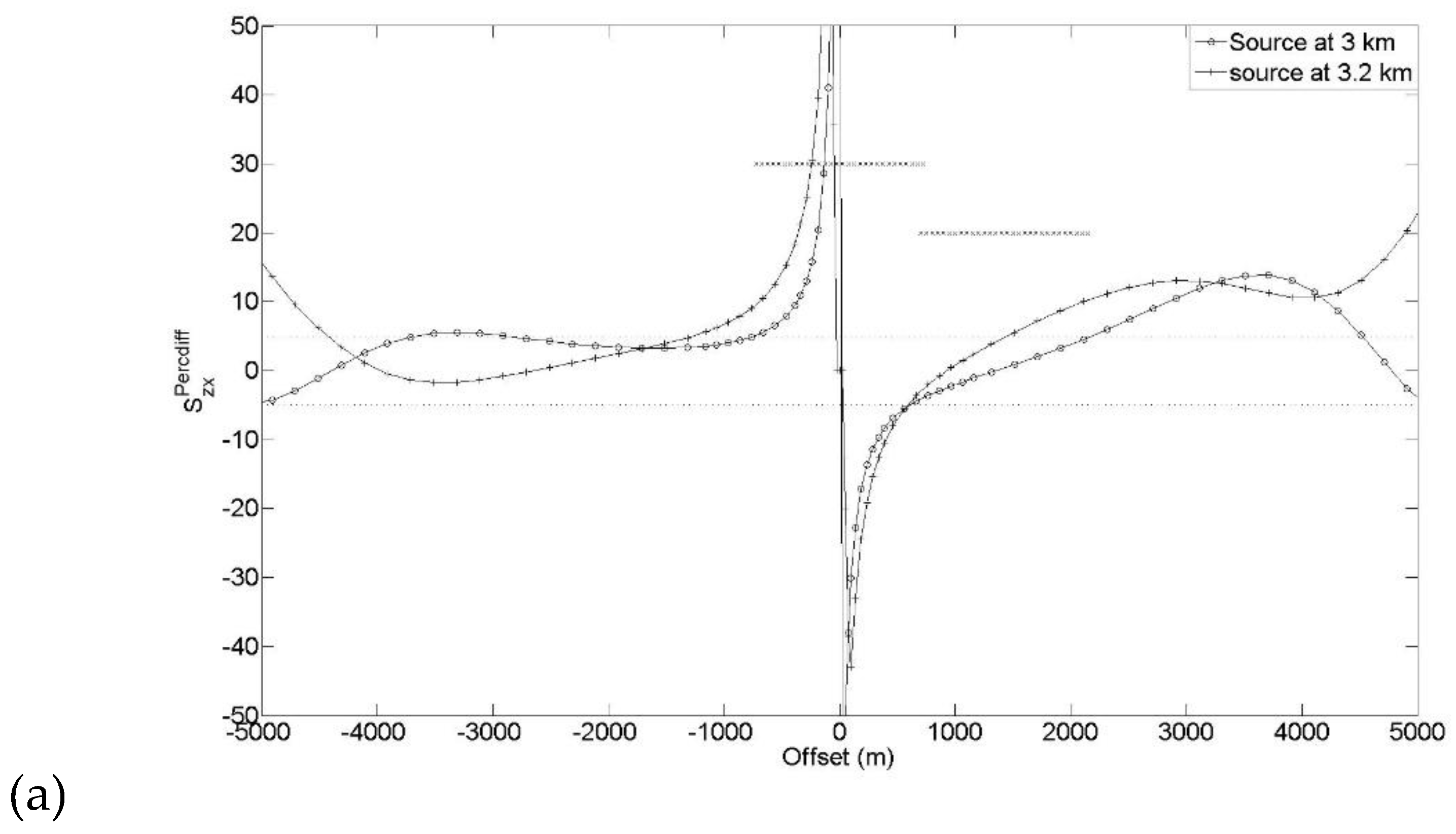
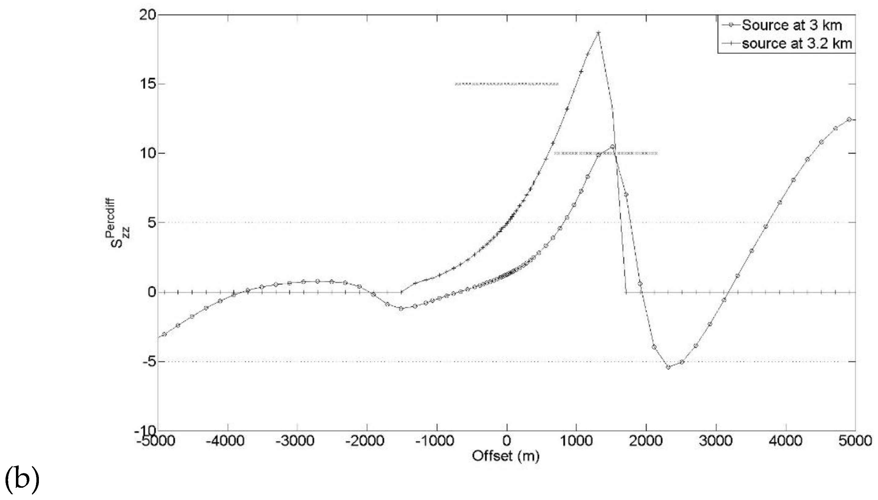
Figure 22.
Percentage differences between centred resistive disk model and that of the half-space reference model of (a) the horizontal and (b) the vertical components of electric field in the xz plane through the transmitter placed at 350 m depth below the seafloor. The locations of source and target are also plotted.
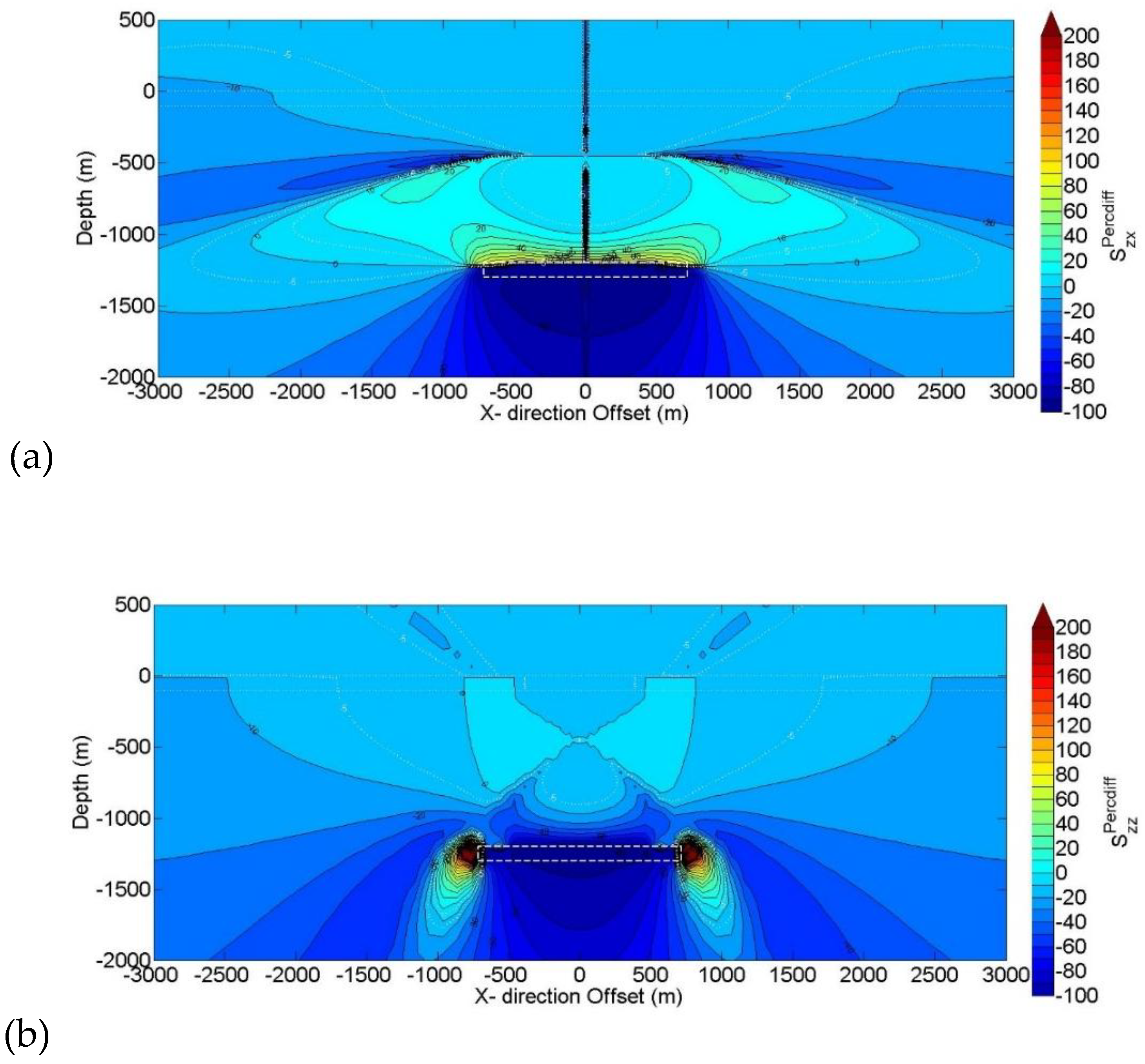
Figure 23.
Contour plots of the dimensionless amplitude of (a) the horizontal and (b) vertical component of electric field at the seafloor, for the centred resistive disk model, plotted as a function of transmitter depth and horizontal transmitter-receiver offset. The location of target is also plotted.
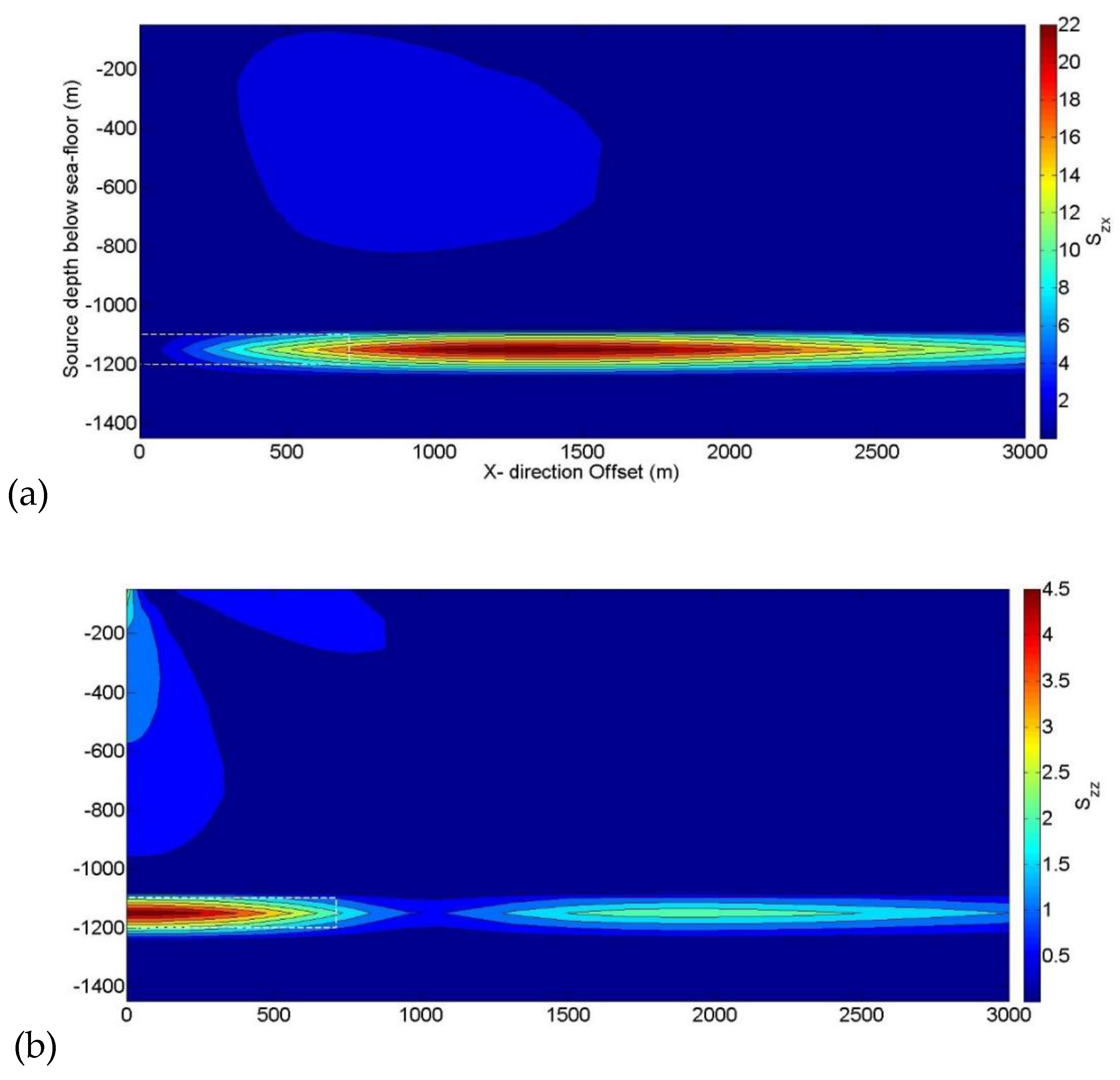
Figure 24.
Contour plots of the percentage difference between centred resistive disk model and that of the half-space reference model of (a) the horizontal and (b) the vertical component of electric field at the seafloor, plotted as a function of transmitter depth and horizontal transmitter-receiver offset. The location of target is also plotted.
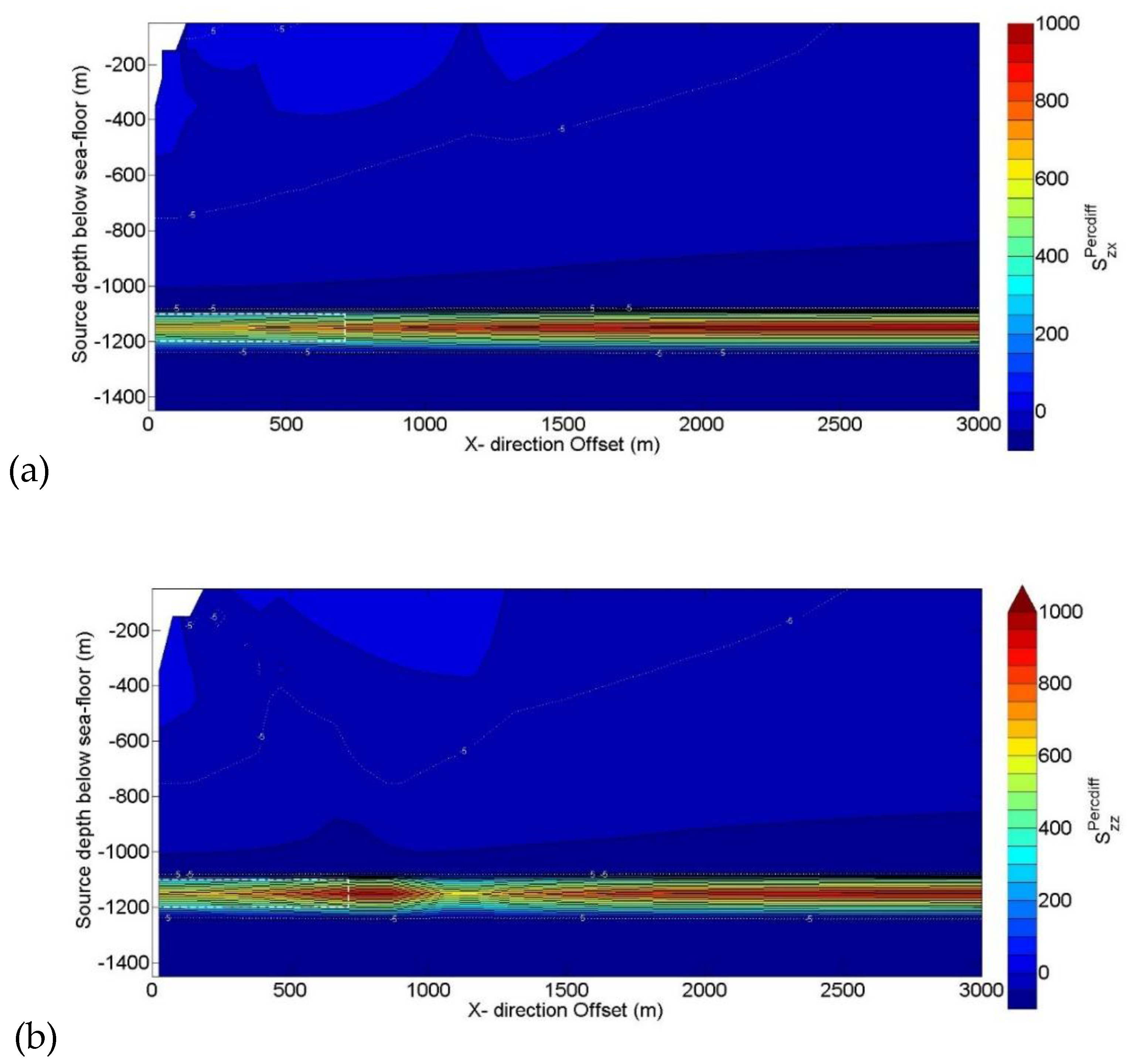

Table 1.
Description of parameters for various standard models used for modelling in the present work. All the models have following parameters in common: Transmitter- 25 m long VED and centred at (0, 0, -1250), Halfspace resistivity – 1 Ω·m, Sea water resistivity – 0.3 Ω·m, Sea water thickness – 100 m, Disk thickness – 100 m, Disk resistivity – 100 Ω·m, Disk diameter – 1425 m (Figure 1). The thin resistive layer model consists of an infinite layer in the x and y directions with thickness of 100 m and resistivity of 100 Ω·m.
| Model | Centre of Disk-1 | Centre of Disk-2 | Centre of layer | ||||||
| X (m) | Y (m) | Z (m) | X (m) | Y (m) | Z (m) | X (m) | Y(m) | Z (m) | |
| Half-space reference | - | - | - | - | - | - | - | - | - |
| Thin resistive layer | - | - | - | - | - | - | 0 | 0 | -1250 |
| Centred resistive disk | 0 | 0 | -1250 | - | - | - | - | - | - |
| Just inside | 700 | 0 | -1250 | - | - | - | - | - | - |
| Just outside | 725 | 0 | -1250 | - | - | - | - | - | - |
| Stacked reservoir | 0 | 0 | -1250 | 1400 | 0 | -1450 | - | - | - |
Disclaimer/Publisher’s Note: The statements, opinions and data contained in all publications are solely those of the individual author(s) and contributor(s) and not of MDPI and/or the editor(s). MDPI and/or the editor(s) disclaim responsibility for any injury to people or property resulting from any ideas, methods, instructions or products referred to in the content. |
© 2026 by the authors. Licensee MDPI, Basel, Switzerland. This article is an open access article distributed under the terms and conditions of the Creative Commons Attribution (CC BY) license (http://creativecommons.org/licenses/by/4.0/).
Copyright: This open access article is published under a Creative Commons CC BY 4.0 license, which permit the free download, distribution, and reuse, provided that the author and preprint are cited in any reuse.


