Submitted:
19 January 2026
Posted:
21 January 2026
You are already at the latest version
Abstract
This study proposes an optimization model for bidding quotations of non-standard automation projects based on historical financial data, aiming to address the subjectivity and instability inherent in traditional pricing methods. Through data preprocessing, feature engineering, model selection, and ensemble techniques, a multi-model collaborative prediction framework is constructed. Combining the strengths of tree models, linear regression, and neural networks, the model employs a residual correction mechanism to refine prediction outcomes.Experimental results demonstrate that the integrated model achieves superior pricing accuracy across projects of varying scales and process categories, significantly enhancing quotation stability and reliability. This research provides a feasible technical pathway for automating non-standard project quotations and holds strong potential for engineering applications.
Keywords:
Non-standard automated projects
; bid quotations
; machine learning
; data-driven
1. Introduction
Bid pricing for non-standard automation projects remains a persistent challenge in engineering project management. Due to high complexity and customization, traditional pricing methods often rely heavily on experience, resulting in significant quotation deviations and unstable predictions. As project scales continue to expand and process requirements diversify, manual estimation approaches can no longer meet modern management demands [1]. To enhance quotation accuracy and mitigate risks, this paper proposes a pricing optimization model based on historical financial data. Through techniques including data preprocessing, feature engineering, and model fusion, it constructs an automated pricing framework tailored to the characteristics of non-standard automation projects. This framework effectively improves quotation precision for projects of varying scales and process complexities, demonstrating strong engineering application value.
2. Research Background
Non-standard automation projects show significant differences in structure complexity, process path, outsourcing ratio, and commissioning cycle, resulting in highly discrete historical financial data with strong non-linear correlations. The cost structure is driven by the fluctuation of material prices, the choice of process schemes, and the changes in the working hours. Inconsistent BOM granularity and different outsourcing fee settlement cycles have further complicated the data modeling.The method of quotation is based on accumulated experience and lacks a quantitative description of the relationship between cost factors, resulting in frequent deviations at the quotation stage for projects of different sizes [2]. Although machine learning can detect hidden patterns in heterogeneous data, it is difficult to apply it to non-standardized projects. In order to improve generalization capabilities, we need more sophisticated feature engineering, data slicing modeling, and model ensemble strategies.
3. Machine Learning-Based Bid Pricing Modeling Approach
3.1. Data Collection and Preprocessing
Data sources comprise historical financial systems, BOM lists, and subcontracting orders. Fields for materials, labor, man-hours, and structural parameters are aligned by project dimension, establishing multi-table mapping relationships via unified primary keys.As shown in Figure 1, missing values are imputed using project-type-specific mean values or process interval interpolation. Outliers are filtered based on quartile-based thresholding [3]. Quotation targets exhibit right-skewed distributions, necessitating skewness correction via Box-Cox transformation:
where represents the original quotation, and is determined by maximum likelihood estimation. Numeric features are standardized using Z-scores and predictions inverse-transformed via Box-Cox
where denotes the original feature, represents the sample mean, and indicates the standard deviation. Field recoding and dimensionality alignment are performed on features from different sources. K-means clustering is applied to slice similar items, using fixed initial seeds to ensure reproducible partitions that may disrupt model training [4].After preprocessing, a structured input matrix is generated and permanently incorporated into the model data version control system.
3.2. Feature Engineering
The feature system is constructed based on project scale parameters, cost drivers, and structural attributes, following the sequence of categorical encoding, dimensionality alignment, and correlation filtering. As shown in Figure 2, material-related dimensions first extract material proportion, outsourced processing ratio, and structural component geometric parameters; labor-related dimensions generate labor-hour gradient coefficients and job composition ratios [5]. Project complexity indices are calculated based on the number of primary structural nodes, number of motion axes, and control unit scale:
where represents the number of structural nodes, denotes the number of motion axes, and indicates the number of control units. The coefficients are derived from historical regression analysis. The schedule pressure index is constructed based on the difference between the planned cycle and the empirical benchmark:
Where represents the project planned cycle, and denotes the benchmark cycle for similar projects. For continuous features, WOE binning enhances monotonicity; for cost features, ratio normalization reduces scale effects; highly correlated variables are filtered using a 0.85 threshold, retaining more explanatory factors. This ultimately forms the feature matrix input to the model [6].
3.3. Model Algorithm Selection
The model architecture comprises linear regression, tree models, and lightweight neural networks, capturing linear and nonlinear relationships among cost factors through differentiated structures [7]. Linear regression serves for baseline alignment, with parameters solved via least squares. XGBoost and LightGBM fit multidimensional interaction features using leaf node growth strategies, with learning rate set at 0.05 and maximum depth fixed consistently at 6 to ensure unified configuration.The MLP employs a two-layer hidden structure with 64 and 32 nodes respectively, using ReLU activation functions and trained via the Adam optimizer. The primary loss function is MAE to enhance robustness against large quotation fluctuations, defined as:
where represents the actual quote and denotes the predicted value. To enhance the model's ability to capture small-scale projects, MAPE is employed as an auxiliary optimization objective:
The final output integrates multiple models through a Stacking architecture, utilizing a secondary regressor to correct residuals and enhance generalization stability.
3.4. Model Construction Framework
The overall architecture comprises an input layer, feature selection layer, base model ensemble layer, and residual correction layer, as shown in Figure 3. The input layer receives structural parameters, cost factors, and derived features. The feature selection layer filters redundant variables based on SHAP weights and correlation thresholds, while performing monotonic binning on continuous features[8] .The base model ensemble layer comprises parallel linear regression, XGBoost, LightGBM, and MLP models. Each model independently optimizes on a unified training set, producing intermediate predictions. The fusion layer employs a stacking-based weighted fusion scheme:
represents the output of the kth model, while denotes the fusion weight learned through a meta-learner within the stacking process, satisfying simultaneously that . To mitigate tail distribution fluctuations, the residual correction layer constructs a lightweight regression model to perform quadratic fitting on the residual . The correction term is then superimposed onto the final prediction as , enabling differentiated fitting for projects of varying scales and enhancing robustness [9].
4. Experimental Design and Results Analysis
4.1. Experimental Dataset
The experimental dataset consists of 812 non-standard automation projects completed over the past five years, covering installation, transport, inspection, and flexible tooling. Stratified sampling by process category ensured balanced cost structures. Forty-two cost and structural components were collected, and preprocessing yielded 28 standardized features, 74.1% of which were continuous. The data were split into 70%, 20%, and 10% subsets, with related projects grouped by shared identifiers to prevent leakage. All samples underwent Box-Cox transformation and Z-score normalization before being stored in a versioned data warehouse for model training access [10].
4.2. Model Training Process
Model training followed a unified parameter management scheme. Base models were trained on the training set, with hyperparameter search and early stopping performed on the validation set. XGBoost used a 0.05 learning rate, max depth of 6, and 0.8 subsampling; LightGBM adopted 31 leaves, a depth limit of 6, and a 0.7 feature sampling ratio. The MLP employed a 64–32 hidden structure with ReLU activation and Adam (learning rate 1e-3). Validation-based early stopping (patience = 50) ensured stable convergence. As shown in Figure 4, tree models stabilized around 120 iterations, while the MLP converged near 180. Checkpoints with the lowest validation MAE were retained for ensemble integration to maintain consistent optimization across models.
4.3. Performance Evaluation Metrics
To assess the accuracy and stability of bid prediction, a four-measure evaluation system was used, which consisted of MAE, RMSE, MAPE, and R ². MAE is a measure of absolute error, which is suitable for situations where there are large quotation ranges in non-standard projects; RMSE is sensitive to fluctuations in large projects, which reveals model bias in high-cost segments; MAPE evaluates relative errors, focusing on predicting the stability of small projects; R ² reflects the ability of the model to adapt to changes in cost structure. In the process of evaluation, the measure is calculated separately for each project size, and the right side is evaluated separately to guarantee the robustness of the model in the extreme cost area. Residual distribution statistics are also introduced to help identify possible systemic bias in errors, and to ensure consistency across the model.
4.4. Experimental Results
To validate model effectiveness, performance comparisons were conducted on the test set for each base model and the ensemble model. Evaluation results are shown in Table 1. The table indicates that the tree model outperforms the linear model in terms of MAE and RMSE, while the ensemble model achieves the best performance across all four metrics. This demonstrates that the multi-model structure effectively mitigates the impact of structural differences between project types.
Table 1 demonstrates that the fusion model exhibits significantly reduced volatility in high-cost zones, with RMSE improvement outperforming individual models, indicating the residual correction module enhances tail distribution performance. To further validate model fitting, Figure 5 displays the scatter plot distribution of predicted versus actual values.Scatter points predominantly cluster near 45°, with deviations concentrated in projects spanning extreme process ranges, indicating high reliability across typical intervals. Analysis of scatter density reveals a slight upward bias in the high-value project segment, consistent with the RMSE differences in Table 1.
Figure 6 presents the error distribution histogram. Errors cluster within the -1500, 1500 ten-thousand yuan range, exhibiting a short right tail, indicating that residual correction effectively mitigates the accumulation of large errors. The column distribution shows good symmetry with no observable systematic bias, demonstrating that the fusion model achieves stable output across different scale intervals.
5. Conclusion
In this paper, a data-driven pricing system based on historical finance data is proposed to solve the problem of bidding and pricing in non-standard automation projects. From data preprocessing, characteristic structure, model choice, and fusion prediction, the system formalizes heterogeneous cost factors into structured representations that quantitatively capture project complexity, schedule pressure, and cost composition. Through the integration of tree, linear, and neural networks, it achieves robust fitting performance for various project types. Combined with a residual correction mechanism, it reduces tail bias caused by extreme cost fluctuations. Overall results show that constructing a multi-model integrated quotation framework for non-standard automation scenarios provides more stable prediction performance in highly discrete cost environments, forming an expandable engineering-based pricing methodology system while offering a scalable foundation for continuous model evolution driven by incremental data accumulation and adaptive algorithm optimization, enabling broader applicability across diverse project categories.
CCS CONCEPTS:
Information systems ~ Data management systems ~ Database design and models.
References
- Zhou H, Gao B, Tang S, et al. Intelligent detection on construction project contract missing clauses based on deep learning and NLP[J]. Engineering, Construction and Architectural Management, 2025, 32(3): 1546-1580. [CrossRef]
- Batini N, Becattini N, Cascini G. Machine learning as an enabler for design automation in engineering-to-order industry[J]. AI EDAM, 2025, 39: e15. [CrossRef]
- Darilmaz M F, Demirel M, Altun H O, et al. Artificial Intelligence-Assisted Standard Plane Detection in Hip Ultrasound for Developmental Dysplasia of the Hip: A Novel Real-Time Deep Learning Approach[J]. Journal of Orthopaedic Research®, 2025, 43(10): 1813-1825. [CrossRef]
- Goetz-Fu M, Haller M, Collins T, et al. Development and temporal validation of a deep learning model for automatic fetal biometry from ultrasound videos[J]. Journal of Gynecology Obstetrics and Human Reproduction, 2025: 103039. [CrossRef]
- Li Z, Cai M, Chen J, et al. Self-supervised representation of non-standard mechanical parts and fine-tuning method integrating macro process knowledge[J]. Computer-Aided Design, 2025: 103954. [CrossRef]
- Shan R, Jia X, Su X, et al. Ai-driven multi-objective optimization and decision-making for urban building energy retrofit: advances, challenges, and systematic review[J]. Applied Sciences, 2025, 15(16): 8944. [CrossRef]
- Tupsounder A, Patwari R, Ambati R, et al. Automatic Recognition of Non-standard Number Plates using YOLOv8[C]//2024 11th International Conference on Computing for Sustainable Global Development (INDIACom). IEEE, 2024: 314-319.
- Rashid C H, Shafi I, Khattak B H A, et al. ANN-based software cost estimation with input from COCOMO: CANN model[J]. Alexandria Engineering Journal, 2025, 113: 681-694. [CrossRef]
- Guo S, Chen Y, Kuang Y, et al. Developing machine learning-driven acute kidney injury predictive models using non-standard EMRs in resource-limited settings[J]. Medical Physics, 2025, 52(10): e70038. [CrossRef]
- Zhang X, Qin M, Cheng T, et al. Intelligent Collaborative Robot Based on DMHF-CNN+ YOLOv7 and Soft Q-Learning in Non-Standard Industrial Parts Assembly[C]//2024 IEEE 4th International Conference on Digital Twins and Parallel Intelligence (DTPI). IEEE, 2024: 401-404.
Figure 1.
Data Preprocessing Flowchart.
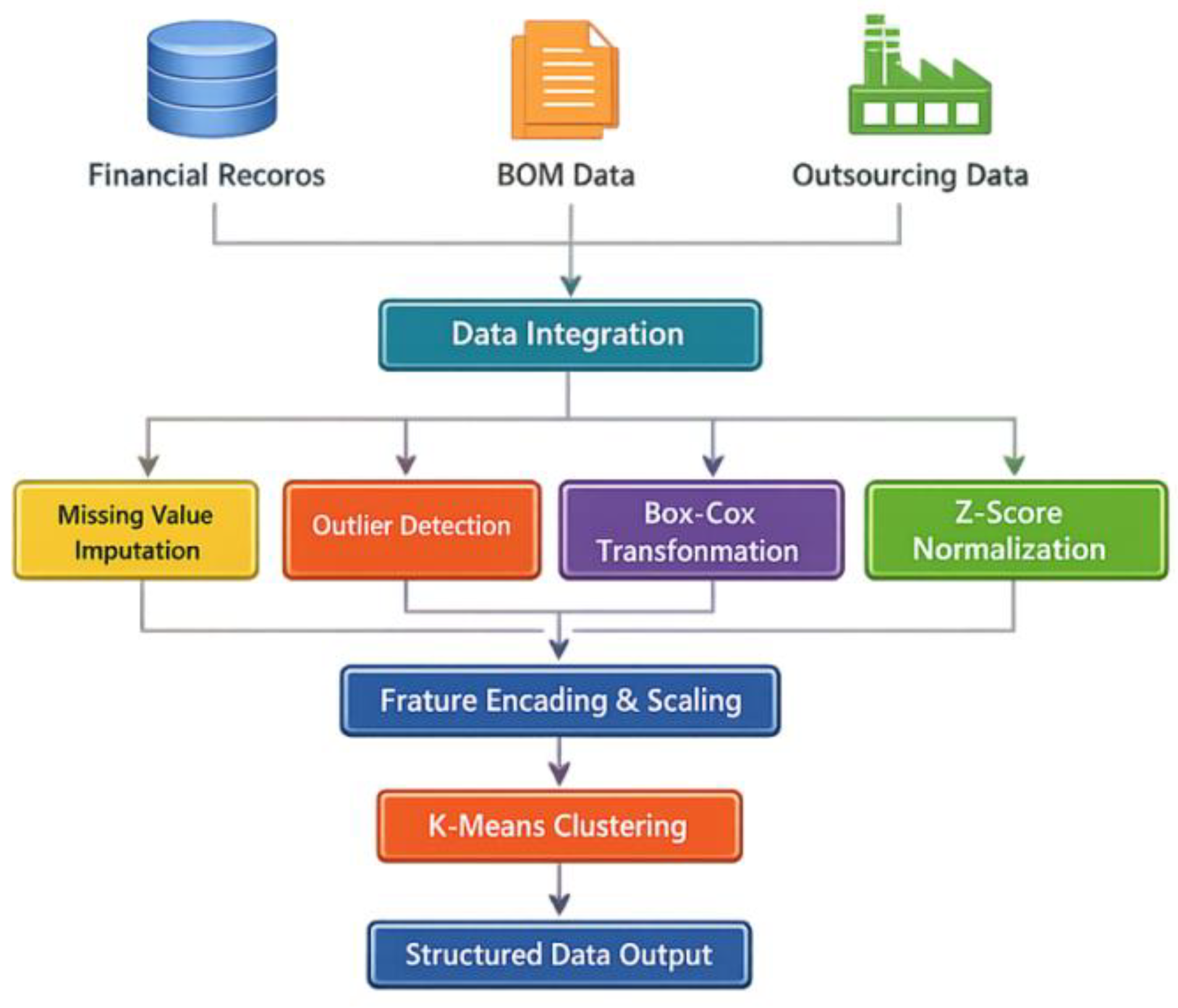
Figure 2.
Feature Correlation Heatmap.
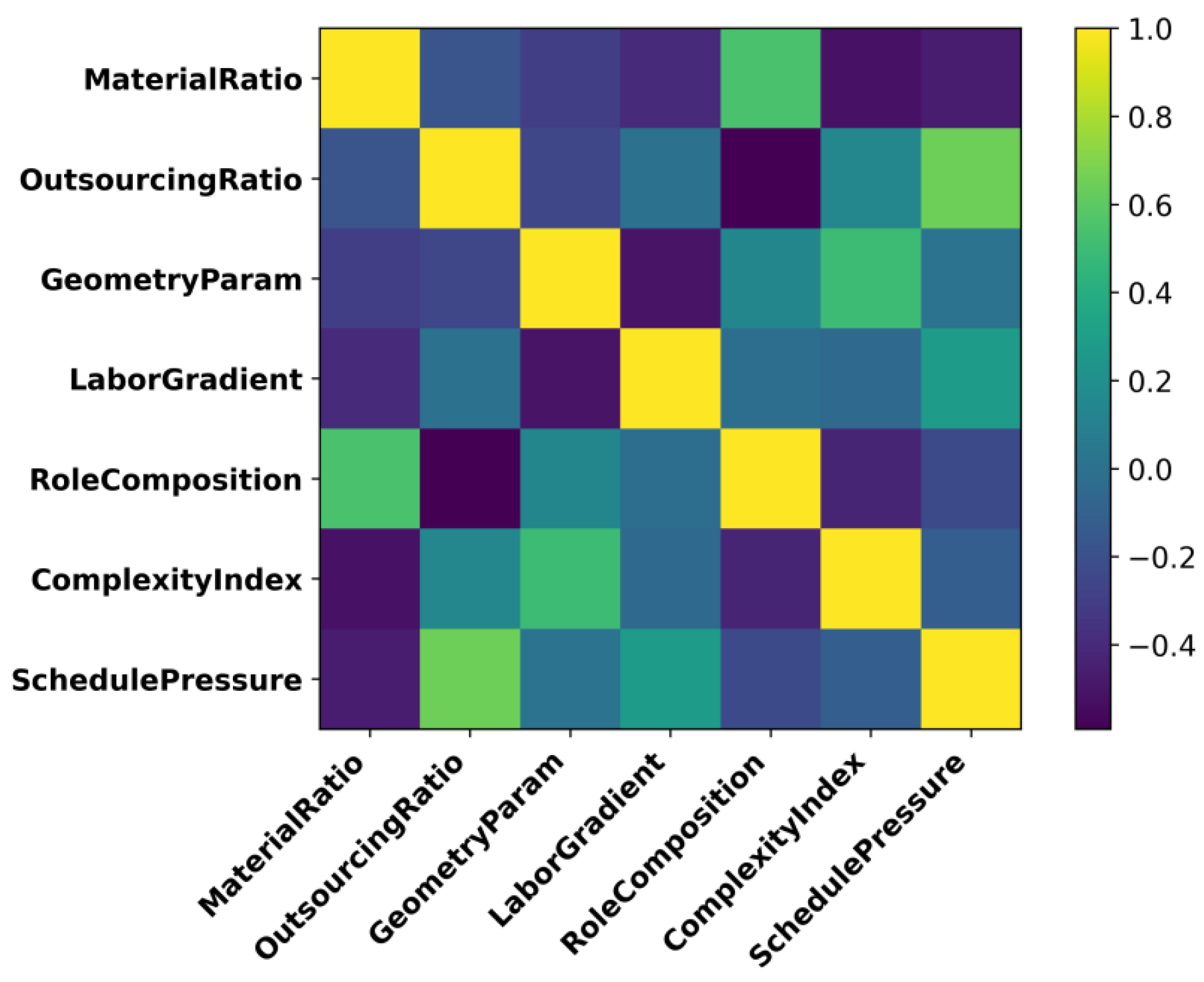
Figure 3.
Overall Model Framework.
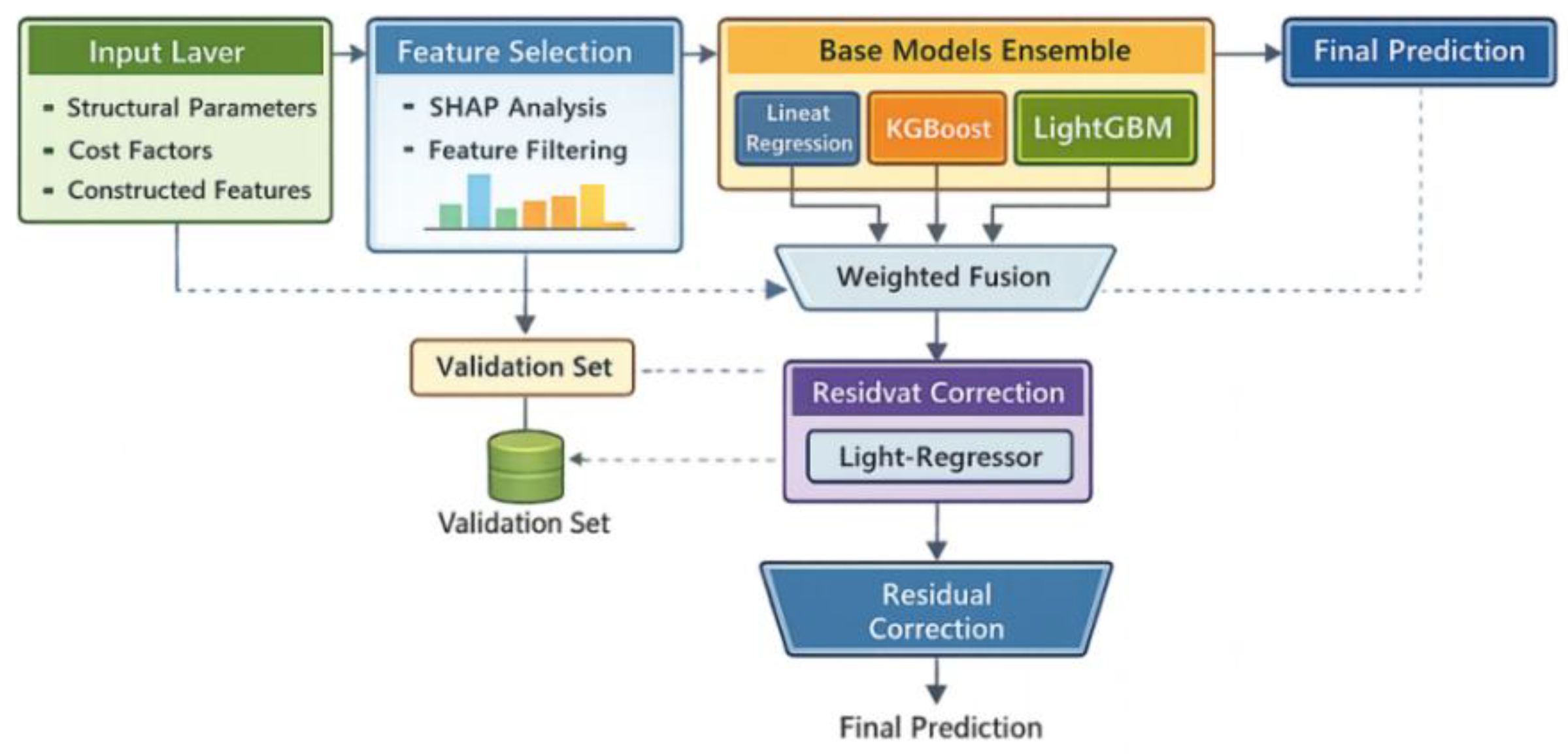
Figure 4.
Model Training Convergence Curve.
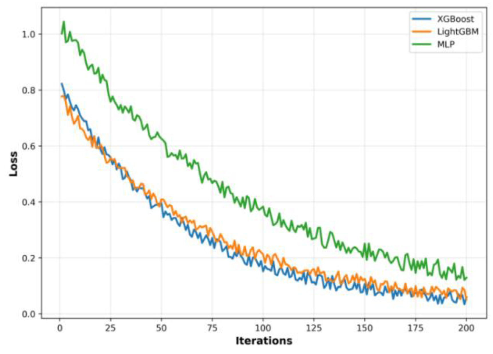
Figure 5.
Scatter Plot of Predicted vs. Actual Values.
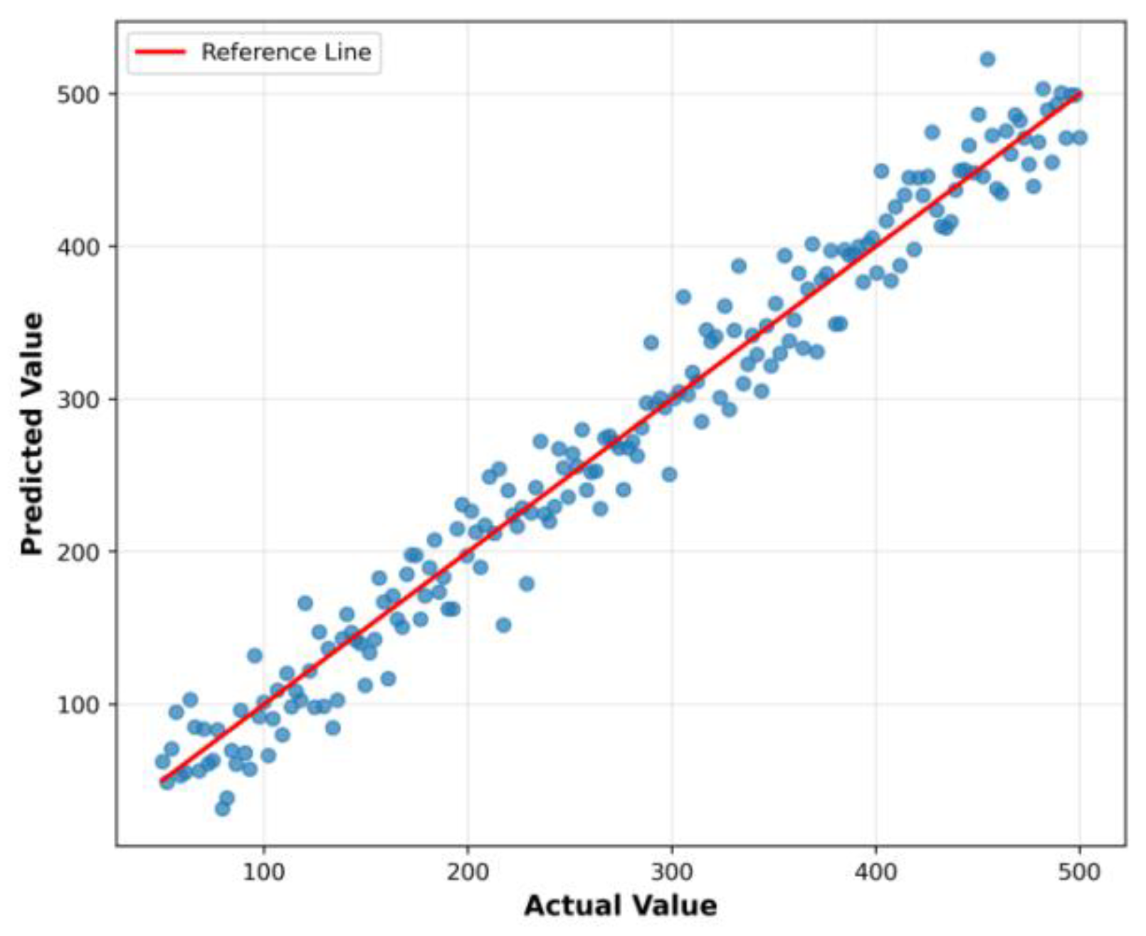
Figure 6.
Fixed-test-set error distribution box plot.
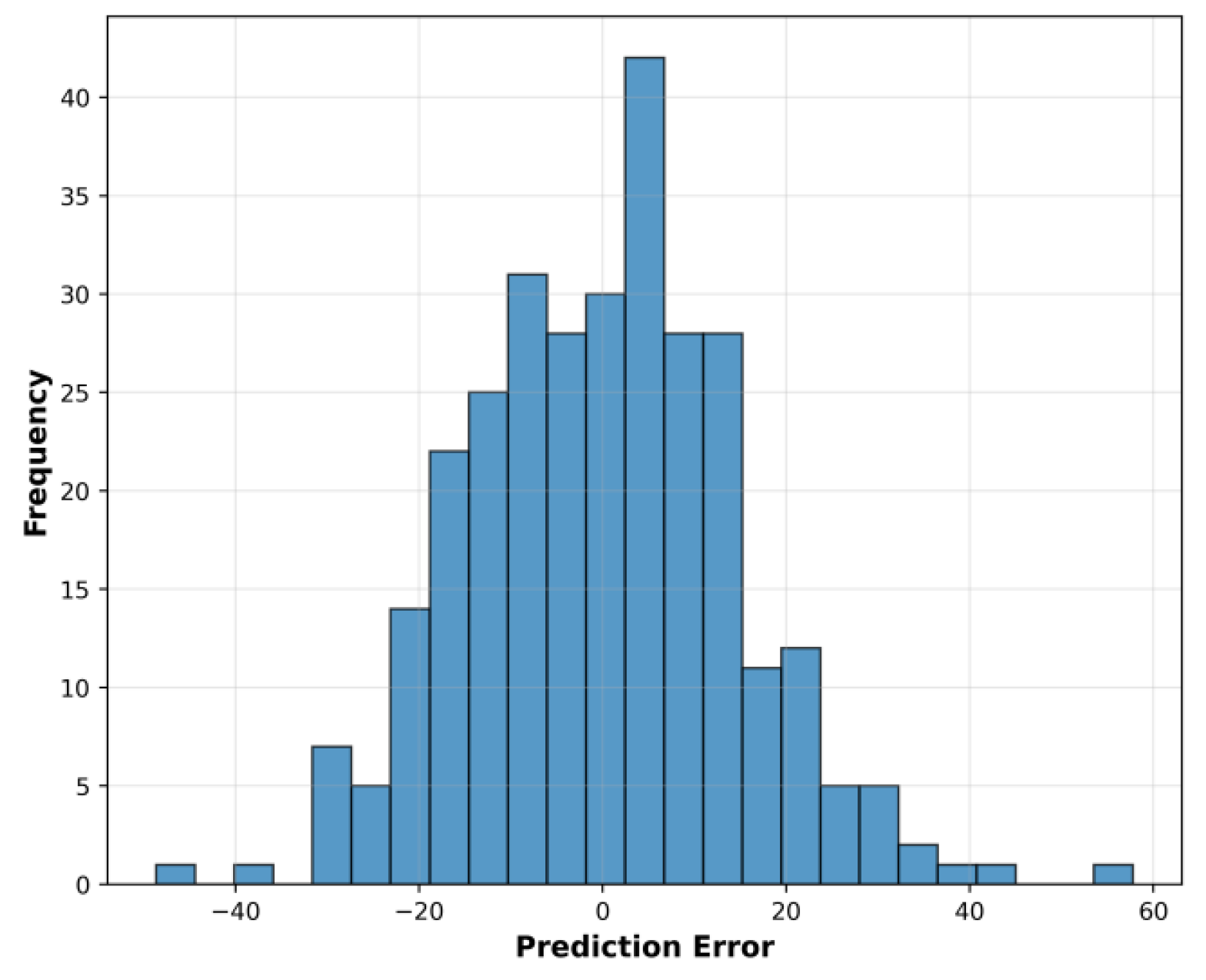

Table 1.
Performance Comparison of Different Models.
| Model | MAE (RMB 10,000) | RMSE (RMB 10,000) | MAPE (%) | R² |
| Linear Regression | 18.42 | 31.27 | 12.8 | 0.76 |
| XGBoost | 11.63 | 22.11 | 7.6 | 0.89 |
| LightGBM | 11.21 | 21.05 | 7.2 | 0.9 |
| MLP | 13.54 | 24.83 | 9.1 | 0.87 |
| Stacking Fusion (Ours) | 9.62 | 18.94 | 6.5 | 0.93 |
Disclaimer/Publisher’s Note: The statements, opinions and data contained in all publications are solely those of the individual author(s) and contributor(s) and not of MDPI and/or the editor(s). MDPI and/or the editor(s) disclaim responsibility for any injury to people or property resulting from any ideas, methods, instructions or products referred to in the content. |
© 2026 by the authors. Licensee MDPI, Basel, Switzerland. This article is an open access article distributed under the terms and conditions of the Creative Commons Attribution (CC BY) license (http://creativecommons.org/licenses/by/4.0/).
Copyright: This open access article is published under a Creative Commons CC BY 4.0 license, which permit the free download, distribution, and reuse, provided that the author and preprint are cited in any reuse.


