
Submitted:
19 January 2026
Posted:
20 January 2026
You are already at the latest version
Abstract
Constant-composition expansion (CCE) experiments provide critical relative-volume and density information describing the thermodynamic behavior of reservoir oils and gases under varying pressure. These properties are vital inputs for hydrocarbon reser-voir engineering, as they impact how oil and gas move through the reservoir during production. However, the need for specialized personnel, high-end equipment and measures taken to ensure safety in handling high pressure fluids often render the CCE experiments expensive and slow. This work introduces a Local Interpolation Method (LIM), a proximity-informed, end-to-end CCE fluid properties prediction AI model that leverages domain expertise and existing PVT data archives to generate surrogate CCE behavior for new fluids, thereby eliminating or reducing the need for completing laboratory CCE tests. Each new fluid is embedded in a compositional–thermodynamic descriptor space, and its response is inferred from a small neighborhood of thermody-namically similar fluids. Within this locality, the LIM combines hybrid local interpola-tion for key scalar properties (such as saturation-point quantities and expansion end-points) with shape-preserving reconstruction of monophasic and diphasic rela-tive-volume curves, enforcing continuity at saturation and consistency between rela-tive volume, density and compressibility. The workflow operates purely at inference time and does not require case-specific retraining. Application to a synthetic database of CCE tests shows that LIM reproduces key CCE features with very good agreement to laboratory data across a range of fluid types, indicating that proximity-based AI mod-elling can substantially reduce reliance on new CCE experiments while maintaining engineering-grade fidelity for compositional simulation workflows. The proposed ap-proach has been fully automated through software so it can be set up and directly uti-lized by the field operators on their own databases to significantly reduce their fluid sampling and laboratory analysis costs. The proposed model does not use others’ data while respecting the data privacy and data ownership.
Keywords:
constant composition expansion
; PVT properties
; reservoir fluids
; local interpolation model
; k-nearest neighbors
; thermodynamic behavior
; machine learning
1. Introduction
When conducting volume calculations and flow simulations in petroleum engineering, fluid properties govern nearly every aspect of system behavior [1,2,3,4,5]. From estimating recoverable reserves to modeling fluid flow in porous media and wellbores, designing surface pipeline systems, selecting separation and processing equipment, and optimizing the overall production system, accurate fluid thermodynamic and transport property data are essential.
Key fluid properties include Pressure–Volume–Temperature (PVT) behavior, rheology, and thermal properties, all of which enter the differential equations governing conservation of mass, momentum, and energy. Among these, PVT data are particularly critical because they describe how reservoir fluids shrink, swell, vaporize, or condense in response to pressure and temperature variations during reservoir depletion, wellbore production, and surface processing [6,7,8,9,10]. Thermodynamic effects such as oil and gas expansion under pressure depletion, gas evolution out of the oil phase for black oils, and liquid condensation in retrograde condensate fluids are major controls on well productivity and ultimate recovery for any given field [6,7,9,10]. Taken together, these phenomena govern multiphase flow behavior throughout the production system, from the reservoir to the surface facilities, and provide the foundation for reliable black-oil and compositional simulation models [6].
Following the acquisition of representative bottomhole samples (BHS) or surface sample (RSS) [6,11,12], laboratory PVT experiments are the primary source of such data, as they map phase and volumetric responses along controlled pressure and temperature paths that are representative of reservoir and surface conditions [12,13,14,15]. Within this suite of tests, the Constant Composition Expansion (CCE) experiment represents the depletion process in which the overall mixture composition is assumed constant [6,12,13]. CCE results are routinely used to tune cubic Equations of State (EoS) and to generate consistent simulation inputs [16,17]. However, CCE testing is also a highly resource-intensive experiment [12,13]: that requires specialized high-pressure apparatus [18]. The CCE test procedures require lengthy stabilization at each pressure step and expert oversight, so each test can consume substantial laboratory time with a corresponding substantial cost. Consequently, only a limited set of depletion paths are typically measured, often only a single path at the reservoir temperature, which motivates the development of surrogate approaches [19,20,21,22,23] that can reproduce the essential CCE-derived relationships with engineering fidelity without requiring additional CCE tests.
Building on this motivation, the AI model presented in this work adopts a Local Interpolation Model (LIM) that infers CCE outputs from rigorously quality-controlled fluids drawn from a synthetic database. Its performance is governed by proximity rather than archive size: predictions are most reliable when the target fluid resides in a “good” neighborhood populated by several highly relevant samples with a CCE study, and gradually deteriorate as the neighborhood becomes poorer (that is, as dBase fluids become less similar in composition/descriptor space). Although CCE tests are performed for both oils and gases, the present study applies the proposed model to reservoir oils.
The approach aligns with industrial practice, where companies typically produce from a specific set of fields and wells and fluid compositions evolve only gradually over time (with successive annual samples often differing by only ~1%). Neighbors are identified via a similarity mapping in composition/descriptor space, and model applicability is reported accordingly: cases associated with weaker neighborhoods naturally yield less accurate predictions, reflecting the reduced relevance of the available neighbors.
This paper is structured as follows. Section 2 reviews the CCE experimental and calculations procedure. Section 3 presents the proposed proximity-informed methodology, including descriptor construction, neighbor selection and the prediction of monophasic and diphasic CCE curves. Section 4 reports the accuracy of the approach using a synthetic database of CCE tests. Section 5 discusses the main findings, limitations and practical implications for compositional simulation workflows, and Section 6 concludes the work.
2. Constant Composition Expansion (CCE)
The constant composition expansion (CCE) experiment, also referred to as Constant Mass Expansion (CME), is a foundational isothermal PVT procedure carried out in virtually all reservoir-fluid studies, irrespective of fluid type. In essence, it establishes the pressure–volume relationship of a fluid as it would be depleted in the reservoir by allowing a fixed-mass sample to expand stepwise while maintaining constant temperature and composition. It provides a direct measurement of the saturation pressure , which marks the onset of gas-phase appearance in oils (bubble point) or liquid-phase appearance in gas-condensates (dew point). In addition to identifying , the CCE experiment records total fluid volume as a function of pressure, from which relative volumes, single-phase densities and, depending on fluid type, properties such as oil compressibility, gas deviation factors and liquid dropout in condensates can be inferred.
The defining characteristic of the test is its closed-system nature: no mass is added or removed throughout the pressure reduction, so the overall fluid composition remains constant. As pressure decreases, the volumetric response, particularly the evolution of relative oil volume and the increase in compressibility just below the bubble or dew point, where exsolved gas or condensed liquid grows, yields critical data for tuning equation-of-state (EoS) models and initializing compositional simulators.
This section begins with a detailed description of the experimental procedure (Section 2.1), outlining the laboratory setup, pressure steps and measurement protocols. This is followed by a discussion of how the raw CCE measurements (pressure and fluid volume) are handled to obtain the engineering properties of interest through appropriate mathematical operations applied to the laboratory data (Section 2.2).
2.1. Lab Procedure
The CCE experiment is conducted in a high-pressure PVT cell equipped with a movable piston and a temperature-control system that maintains the chosen test temperature, typically close to the reservoir temperature. Commercially available PVT cells allow for direct measurement of the liquid and vapor volumes and reveal the first visual sign of the incipient phase, i.e. first bubble or drop through still and video pictures as well as through direct operator visual observation.
A sample representative of the in-situ reservoir fluid is first prepared and charged into the PVT cell. The temperature-control system is then set to the desired test temperature and the system is allowed to reach thermal equilibrium. The fluid is initially pressurized to a high pressure condition (typically reservoir pressure or higher) where it is known to be single-phase: a homogeneous liquid for an undersaturated oil or a homogeneous gas for a gas condensate (Figure 1). This initial state lies on the single-phase branch of the pressure–volume (PV) curve.
Subsequently, a pressure depletion sequence proceeds in discrete pressure steps. The operator withdraws the piston by a calibrated increment, increasing the cell volume and causing the pressure to reduce at constant temperature and overall composition. After each step, the fluid in the cell is vigorously mixed rather than being left undisturbed to insure equilibrium between vapor and liquid phases (in the two-phase region). This procedure continues until both pressure and phase appearance have stabilized. At every equilibrium step, the lab operator, supported by equipment that automates the procedure, measures the cell pressure, and the total cell volume. These two values are the raw experimental data of any CCE test, and they define the measured PV relationship for the fixed-mass sample. All subsequent engineering properties (relative volume, compressibility, etc.) are obtained by post-processing these measurements.
As long as the pressure remains above the saturation pressure, the sample appears as a single uniform phase, either oil or gas, and only pressure and total cell volume are recorded. As the piston is gradually withdrawn and the pressure is lowered, the operator looks for the first visible indication of a second phase. For an oil, this is the appearance of gas bubbles within the liquid, whereas for a gas, it is the first liquid droplets or condensate haze in the gas phase or along the cell wall. The equilibrium pressure and volume at which this second phase first appears is recorded as and .
Below , the experiment continues with further calibrated expansions at constant composition. At each new equilibrium step, the laboratory again records the stabilized pressure and total cell volume. In a visual PVT cell, where two phases are now present, the volumes of the liquid and vapor phases are also read directly from the cell and reported as liquid and gas volumes. Thus, for sub-saturation conditions in a visual CCE test, the raw record consists simply of pressure, total cell volume and the measured liquid and vapor volumes at each step.
For an undersaturated oil, this sequence of steps is illustrated schematically in Figure 1. The five frames represent successive equilibrium conditions in the CCE experiment. At , the fluid in the cell is a single-phase oil (shown in green). After a first expansion to , the piston has been withdrawn slightly, the cell volume has increased and the pressure has decreased, but the sample is still a single-phase green oil. At both and , the laboratory records only pressure and total cell volume. When the pressure reaches , the bubble-point condition is attained, and the first small gas bubble (red) is formed within the green oil. This is the first visual indication of the second phase and defines the experimental saturation pressure.
Further expansions to and lead to a clearly two-phase system, with a red gas cap at the top of the cell and a green oil layer below. At each of these sub-saturation steps, the laboratory measures the stabilized pressure and total cell volume, and, in a visual cell, directly records how much of that total volume is occupied by oil and how much by gas. As pressure decreases from to , the gas cap grows while the oil layer shrinks, and the corresponding change in total and phase volumes captures how rapidly gas evolves from solution as depletion progresses towards surface conditions.
The outcome of the CCE procedure is therefore a set of equilibrium measurements, pressure, total cell volume and, in visual cells, liquid and vapor volumes at each step. For oils, the break in slope of the volume curve with pressure (indicative of the change in system compressibility) is typically used to estimate both and . For gas condensates, the two-phase liquid volume data is typically extrapolated back to zero percent liquid to estimate the dew point. This procedure ensures that, unless the pressure is reduced very slowly, the hysteresis effect which leads to erroneous saturation pressure estimation is tackled.
2.2. Data Handling
Building on the equilibrium measurements obtained from the CCE test, this section describes how the raw pressure–volume data are transformed into relative volumes and single-phase properties through a consistent data-handling workflow. For consistency with the scope of this study, the discussion in this section refers to reservoir oils.
Once the saturation pressure has been identified, all volumetric measurements are cast in terms of dimensionless relative volume,
where, is the total cell volume measured at pressure , and is the total cell volume recorded at the saturation pressure . This normalization takes the saturation state as reference. Above saturation, describes the mild expansion of the relatively incompressible single-phase fluid with decreasing pressure. Below saturation, it captures the stronger apparent expansion caused by the growth of the released gas phase in oils.
Quality control of the curve is performed separately in the monophasic and two-phase regions. In the single-phase region, the is expected to follow a smooth, monotonic, weakly curved trend characteristic of isothermal compression of a homogeneous fluid. To enforce this behavior, the data are fitted with the Tait equation [24], used here as a smoothing and regularization tool,
where, the parameters and control slope and curvature of the fit model. Note the Tait equation is applied to and constrained to honor the experimental pair . The resulting Tait curve provides a smooth, internally consistent representation of the single-phase volumetric behavior. Measured points that deviate significantly from this trend are interpreted as unsteady or misread and are discarded. All single-phase volumetric properties in this work are derived from the Tait-smoothed relative-volume curve.
In the two-phase region, the Tait equation is no longer applicable. Instead, the data are screened using the Y-function
which is expected to vary approximately linearly with pressure. Systematic departures from this linear behavior flag sub-saturation points affected by interface-reading errors or incomplete equilibration. These points are reviewed and, where necessary, adjusted or removed without altering the value of .
Once quality control has been applied, additional one-phase properties are obtained directly from the smoothed relative-volume data. The density at saturation is
where, is the known total sample mass charged in the PV cell, and the oil density at any pressure follows from inversion of the relative volume,
Finally, since the Tait equation provides a smooth analytic representation of the single-phase relative-volume curve, its derivative can be used to obtain a closed-form expression for the point isothermal compressibility, avoiding numerical differentiation. Differentiation gives
3. Methodology
3.1. Overview of the Workflow
The proposed workflow generates Constant Composition Expansion outputs for a target fluid by combining the LIM for pointwise PVT properties with shape-preserving, k-nearest-neighbor (kNN) blending of preprocessed CCE curves in a PVT database. The entire procedure operates at inference time: the database is prepared once, and every new prediction is obtained by using precomputed neighbor information properties, derivatives and normalized curve shapes without any retraining.
The methodology comprises three main components. First, each fluid is embedded in a common descriptor space, and a set of thermodynamically relevant neighbors is identified using robust multi-metric distances which emulate the fluid similarity criteria of a domain expert. Second, LIM is used to produce pointwise endpoint predictions at distinct pressures (for example, relative volumes, densities or pressures at specific expansion levels), combining domain-driven derivatives with data-driven corrections. Third, full CCE curves are reconstructed in normalized space by blending the shapes of neighboring fluids curves, and then de-normalizing them with the LIM endpoints, under explicit monotonicity and continuity constraints. This procedure ensures physically sound, physics-backed and domain experts assisted prediction of all CCE PVT curves. The following subsections describe these stages in more detail and show how they connect to form a consistent AI model.
3.2. Descriptor Space and Multi-Metric Neighbor Selection
In the database-preparation stage, each fluid is represented by a descriptor vector that concatenates composition and key thermodynamic or characterization scalars. In addition to the detailed mole fraction vector z (e.g. , ..., ), the descriptor includes reservoir temperature and saturation pressure , as well as stock-tank and reservoir fluid molecular weight, stock-tank density, API gravity and other scalars that summarize fluid quality and volatility. The latter are properties from a traditional fluid compositional analysis. These features are scaled and, where appropriate, reduced via methods such as component lumping, Principal Component Analysis (PCA) or nonlinear embeddings so that multiple distance metrics can be defined on comparable numerical ranges. For composition and reservoir temperature, these features are normalized according to their significance to the predicted PVT property. This is quantified through sensitivities , where denotes the PVT property to be predicted and is the jth descriptor component. For each metric , a pairwise distance matrix is computed across the CCE database and converted into an empirical distribution of distances, expressed as percentiles. This distribution acts as a “fingerprint” of the database utilized. The narrower the spread, the greater the similarity among the fluids. A bimodal distribution indicates two distinct fluid clusters, for example fluids originating from two different fields.
Neighbor selection for a given target fluid is then carried out in this multi-metric percentile space, based on a stochastic approach to avoid strict deterministic calculations. Firstly, matrix is constructed containing all distances between any pair of fluids in the archive. The histogram of those distances acts as a “fingerprint” of the dBase upon which future predictions will be based on. This distribution is shown in Figure 2 below, marked in cyan color.
At inference time, the only information required to execute this step is the target’s descriptor vector d. The target is compared against all archived fluids, yielding a set of percentile ranks that quantify how close each candidate neighbor is. The histogram of the distances of a test fluid against the dBase is also shown in the same Figure in orange color. Clearly, the more shifted to the left-hand-side of the fingerprint the new test fluid is, the more “familiar” that fluid is with respect to the dBase entries, hence the safer is expected to be the prediction of its PVT properties.
Since the closest neighbors of a test fluid are the ones that contribute most to the PVT values predictions, confidence increases when a sufficient number of such neighbors can be traced within the left-most part of the cyan histogram. Indeed, when at least 5 neighbors can be identified within the 5% percentile of the dBase fingerprint histogram, the test fluid is considered to be a “familiar” one and is labeled as a “Tier 1” test fluid. Similarly, when the 5 closest neighbors distances are limited above 5% but below 10% of the fingerprint, the fluid is labeled a “Tier 2” one. The requirements for the next tiers have been defined with progressively looser consistency thresholds, indicating reduced or limited confidence on the presence of similar PVT studies in the dBase which could drive the prediction system and provide confident predictions. The resulting distribution of a test fluid is summarized into a Tier 1–3 label that provides a compact measure of analog availability and overall similarity strength in the archive. The black lines in Figure 3 correspond to the distances between a test fluid and its closest neighbors in the archive. Clearly, a sufficient number of sufficiently close neighbors can be identified thanks to the location of the dBase fluids to the test one, i.e. the black lines lie within the 5% percentile of the fingerprint.
Since more than one distance metrics have been utilized, a robust distance score for the test fluid is constructed by aggregating percentile ranks across all metrics while discarding the single worst one, thereby penalizing fluids that are consistently dissimilar across different views of the space while avoiding over-sensitivity to a single noisy metric. Neighbors are ranked by this “robustness” score, and the prediction engine restricts attention to a small neighborhood (typically up to the five top-ranked neighbors), which effectively defines a local trust region around the target in descriptor space. This design enforces a strict locality principle: predictions are driven by nearby fluids that lie in the same compositional–thermodynamic regime rather than by the global spread of the archive. On top of this neighbor structure, LIM provides pointwise predictions, and the curve surrogate re-uses the same selected neighbors and their associated multi-metric distances.
It is important to note that this neighbor-selection stage is independent of the particular output being reconstructed: it depends only on d and the PVT tests archive. Property-specific quantities that may be available for the target fluid and are used later as reconstruction constraints (e.g., endpoint measurements such as at a high pressure ceiling for the monophasic branch, or diphasic/event anchors used to parameterize . do not enter the similarity search and therefore do not affect neighbor ranking. On top of this neighbor structure, LIM provides pointwise predictions, and the curve surrogate reuses the same selected neighbors and their associated multi-metric distances.
3.3. Hybrid Local Interpolation Model (LIM) for Pointwise Properties
Within the trust region defined in Section 3.2, the hybrid LIM framework provides point predictions for scalar PVT quantities. For each endpoint of interest (e.g. density at saturation, or the pressure at which ), the model does not learn a global mapping over the entire fluid space. Instead, it uses a small set of thermodynamically similar “anchor” fluids and approximates the property of the target fluid by local first-order Taylor expansion corrections around each anchor.
For a given anchor with known property value , the domain-driven leg of LIM constructs a Taylor expansion in raw composition and temperature that is the fundamental properties,
where, is the predicted PVT property for the test fluid, are compositional coordinates, and is number of components. The sensitivities and are pre-computed once per anchor by finite-difference perturbations in an inhouse PVT simulator and scaled by property-specific gain factors. Because these derivatives are computed for fluids in the database (i.e., for the anchors) rather than for the test fluid, they are evaluated once per anchor, stored, and subsequently reused to apply Eq. (3.1) for any target fluid that selects the same anchor during inference.
Each term corresponds to the correction that needs to be applied at property of the test fluid , compared to that of the neighboring fluid . For example, consider the conventional Differential Liberation property at . In the Taylor step, the term accounts for the change in due to the temperature difference between the two fluids, while holding composition fixed. The sum of these terms provides a single vector-based correction that moves the anchor’s known property toward the target while remaining firmly grounded in thermodynamics. A simplified graphical representation of Eq. 3.1 is given in Figure 3, where all components contribution has collapsed to a single dimension.
To capture fluid-to-fluid variability that is not fully explained by (z, T), such as effects associated with isomers, component-to-component interactions or heavy-end indicators, the model augments the domain-expert Taylor step with a data-driven correction. Let denote and auxiliary block consisting of available PVT properties (e.g., ). Most of those properties are directly obtained from a standard compositional analysis. Within a short radius around the test fluid, called a trust region, LIM assumes that the dependence of the target property to be predicted on is locally linear and estimates a neighborhood-specific coefficient vector from data. Specifically,
and vector is obtained by fitting the pairwise relation
over all pairs of neighboring fluids , lying in the trust region, in a ridge-regularized least-squares sense. This optimization minimizes the mismatch between observed property differences and those predicted by the local linear model in the augmented input space. In the hybrid formulation, the resulting c-based correction is combined with the simulator-derived Taylor correction in (z, T). In the hybrid formulation, the final correction from an anchor to a target is obtained by
Figure 4 provides a geometric interpretation of this hybrid Taylor step. In the left panel, the green bar represents an anchor fluid at its known composition, temperature and property value , while the blue bar represents the target fluid at its own coordinates, with unknown . The green horizontal plane corresponds to the composition–temperature input space. Composition–temperature differences define a lateral shift from the anchor to the target, and the simulator-derived derivatives produce the corresponding vertical correction . The additional characterization axis introduces a further shift and an associated vertical adjustment based on the locally learned . The thin blue arrow from the top of the green bar to the top of the blue bar summarizes this combined, vector-valued correction.
The right panel depicts the neighborhood structure in the trust region: the target fluid lies at the center, surrounded by anchor fluids inside the dashed circle. The colored arrows between neighbors indicate that the same set of gradients is optimized to explain not only corrections from each anchor to the target, but also transitions between anchors themselves, enforcing local consistency.
Each anchor-specific step is magnitude-limited to avoid unphysical extrapolation, and outlier estimates are rejected using a median-absolute-deviation criterion when at least three neighbors are available. The remaining corrected values are finally blended into a single scalar PVT value prediction using distance-based weights, so that anchors closest to the target in the sensitivity-weighted descriptor space dominate the estimate while more distant ones act only as mild regularizers. In this framework, the final prediction of PVT property is given by the weighted average of the neighboring fluids property values :
where
The exponential term ensures proper decay of the weighting factors along the distance between the test fluid properties and those of its neighbors. This hybrid LIM prediction is used consistently for all scalar endpoints required by the CCE reconstruction described in the subsequent Sections.
In summary, the developed methodology is described graphically in Figure 5. The effect of the hybrid step has been omitted to keep the workflow simple. Firstly, when a test fluid arrives, its input (i.e. composition, temperature and auxiliary PVT properties) are placed on the fluids space map (a). The dBase fluids are similarly placed on the same map (b). Subsequently, the trust region is defined to identify by means of the neighboring criteria discussed above and the PVT value at each neighboring fluid is recorded (c). The Taylor step is then applied to extrapolate the neighbors PVT values towards the test fluid (d). The extrapolated values differ due to the variance in the distance between the test fluid and its neighbors as well as due to the noise present in experimental data. To account for the contribution of each neighbor’s prediction to the weighted one, the distances are computed (indicated by the connecting lines thickness in (e)), and the weighted average, that is the finally predicted PVT property value is obtained (f).The workflow further demonstrates the inspiration of the proposed methodology from the human/domain expert’s approach to predict the PVT values of a test fluid when a reservoir fluids PVT database is available.
4. Application in CCE Predictions
4.1. Monophasic Relative Volume and Density Above Saturation
The single-phase (monophasic) branch of the CCE relative-volume curve, denoted , is treated in a physics-informed manner. For each database fluid, the measured CCE points above saturation are first quality controlled and then fitted with the Tait model described in Eq. 2.2. This produces a smooth representation of over the stabilized monophasic range while filtering measurement scatter. This preparation step is performed once for the archive and is repeated in the same way whenever new fluids are added.
To make the monophasic curves directly usable by our model, each fitted curve is evaluated on a common pressure grid between and a fixed high-pressure ceiling . The resulting sampled curve is then stored in a normalized, dimensionless form so that all fluids share identical anchors: and . In the implementation used here, this yields an 11-component vector per database fluid. This vector encodes only the shape of the monophasic expansion (independent of absolute scale), which allows meaningful blending across neighboring fluids.
When a new test fluid arrives, the objective is to predict its monophasic relative-volume branch for . What is known for the test fluid is the saturation anchor and one additional measurement at some pressure . Figure 6 illustrates this situation, where the saturation anchor at and the additional monophasic measurement at provide the physical reference values used for reconstruction. The test fluid is first embedded in descriptor space and its neighborhood is identified as described in Section 3.2. A kNN model then predicts the normalized monophasic shape on the same 11-point grid by distance-weighted blending of the neighbors’ normalized vectors.
To use the measured point in the denormalization step, its normalized pressure coordinate is obtained directly from the known pressure anchors and the fixed high-pressure ceiling . However, the corresponding normalized relative-volume value is not available explicitly because the prediction is provided only on the discrete 11-point grid. Therefore, a Tait-like curve is fitted to the 11 predicted points in normalized space and evaluated at to obtain .
The remaining step is to recover the physical scaling of the curve for the test fluid. In the adopted normalization, the only unknown needed to denormalize the entire monophasic branch is the high-pressure endpoint . This endpoint is identified by enforcing consistency with the available measurement . while preserving the predicted normalized shape. Using the denormalization mapping
and evaluating it at yields
Now that is available, both endpoints are well defined and the whole curve can be fully reconstructed using denormalization. Single-phase density along the CCE path is reconstructed in a manner that is exactly consistent with . For the test fluid, what is available is one additional monophasic measurement . Figure 7 illustrates this analogous setting for density, where and serve as physical anchors in the monophasic region.
As with relative volume, kNN first predicts a normalized density shape on the same 11-point pressure grid by distance-weighted blending of neighbors’ normalized density vectors, producing predicted pairs in the range. The normalized pressure coordinate is obtained directly from and .
Let denote the (unknown) density at the fixed high-pressure ceiling. By considering the direct relationship between and and applying at the known pressure point , i.e.
Replacing back to the first equation:
In this way, the relative volume and density curves are tightly coupled, and the analytic derivative of the Tait relation provides a closed-form expression for the effective isothermal compressibility, avoiding additional numerical differentiation (Eq. 2.6). These monophasic reconstructions then serve as the upper anchor for the diphasic branch below saturation.
4.2. Diphasic Relative Volume Below Saturation
Below the saturation point, the diphasic branch of the relative volume, , is reconstructed in an inverse-anchored fashion to match the structure of the database and to stabilize behavior at large expansions. In the archival processing, each sub-saturation CCE trace is converted to a representation defined on a uniform grid rather than a uniform pressure grid. For each fluid, the pressure at which is inferred from the measured points using linear or low-order polynomial interpolation, depending on data availability, and the curve is truncated at this inferred endpoint. The pressure axis is then normalized so that the bubble point maps to zero and the pressure at maps to one, while the axis is normalized so that corresponds to zero and to one. A simple monotone functional form (quadratic when exactly three points are available, rational when four or more points exist) is fitted in this normalized space, and evaluated on a fixed grid of expansion levels between and . Monotonicity checks are enforced, and fluids for which a physically acceptable fit cannot be obtained, are discarded from the database.
For the test fluid, the pressure at is not measured and is therefore treated as an endpoint to be predicted by LIM (Figure 8). Once this endpoint has been estimated, the diphasic branch for the test fluid is constructed on the same normalized grid by blending neighbor curves in space. At each normalized expansion level, pressures from neighboring fluids are combined with distance-based weights, and the resulting sequence is smoothed, where necessary, to enforce a strictly decreasing pressure profile with increasing relative volume. The final curve is obtained by mapping the normalized pressure axis back to dimensional pressures using the anchors at and and by inverting the monotone mapping between expansion and pressure so that the curve connects continuously to at the bubble point and exhibits the expected increase in relative volume as pressure decreases.
4.3. Curve Alignment and Error Evaluation
When performance comparisons between predicted and laboratory CCE curves ( and ) are required and the two curve vectors correspond to different grid pressure points, the difference in tabulation grids is handled explicitly. Because the archival and reconstructed curves are defined on different primary axes (uniform pressure levels for , uniform relative-volume levels for ), one of the two curves is re-gridded so that residuals are computed at common abscissa values. For , the predicted curve that terminates at the lower value of is interpolated onto the lab curve’s pressure grid so that the comparison remains confined to the shared pressure range and does not rely on extrapolation in the high-expansion region, where sensitivity is greatest. The error metrics mean absolute error, mean absolute percentage error, and maximum absolute deviation are then computed on this common grid.
Overall, the methodology combines a physically grounded parametrization of CCE behavior with a strictly local, proximity-informed interpolation scheme. Endpoints are provided by LIM through hybrid domain- and data-driven Taylor corrections, while full curves are reconstructed from neighbor shapes in normalized space and then brought back to dimensional form under explicit continuity and monotonicity constraints. This architecture ensures that the surrogate AI model respects the main thermodynamic structure of CCE experiments, concentrates accuracy where data density is highest, and remains directly usable in EoS tuning workflows without requiring additional CCE tests for new fluids.
5. Results
5.1. Fluidsdata Database
A set of CCE dataset was curated from varieties of literature sources including data synthesis that utilized vast experience of the authors. Care was taken to abide by the known thermodynamics principles while synthesizing and perturbing data at diversified conditions. The synthetic database used in this work should “resemble” the real datasets.
5.2. Results
To evaluate overall predictive performance of the LIM model, leave-one-out cross-validation was performed on the CCE data archive. In each run, one fluid is treated as an unseen test fluid, while all remaining fluids provide candidate neighbors in descriptor space. For every test fluid, the workflow infers the monophasic and diphasic CCE branches and compares the inferred curves against laboratory measurements on a common pressure grid. Curve accuracy is quantified by the mean absolute percentage error (MAPE, %) computed for each fluid as the mean of the pointwise absolute percentage errors along the corresponding curve. In parallel, parity plots are used to assess pointwise agreement between predicted and laboratory values aggregated over all pressure-grid points for the Tier 1–3 population, which represents the majority of the archive (≈77%) and corresponds to well-populated neighborhoods in descriptor space where close neighbors are available and robust accuracy can be expected. The accompanying histogram and cumulative probability distribution (ECDF) panels summarize the distribution of per-fluid curve MAPE and report the 95th-percentile error level.
To illustrate inference quality across neighborhood strengths, three representative test fluids were selected, 10325 (Tier 1), 10261 (Tier 2), and 10459 (Tier 3), ordered by neighborhood quality as determined by the tiering procedure in Section 3.2. Tier 1 corresponds to a dense, highly similar neighborhood in descriptor space, whereas Tier 3 indicates weaker local support. Example inferred monophasic relative-volume curves and their pointwise relative-error profiles are shown for these selected fluids in Figure 9. In all tiers, the inferred closely follows the laboratory curve across the single-phase pressure range, with deviations that remain smooth and small even for Tier 3.
To demonstrate the performance of the domain-expertise aspect of the neighbors selection criterion developed in this work, the normalized curves of the first test fluid (10325) are illustrated in comparison to that of its closest neighbors in Figure 10. Referring to the figure, the test fluids normalized relative volume curve (which is known as the selected test fluid is used as a test point) is shown in red. Light grey is used to show the normalized curves of all fluids within the available VVE studies archive. Finally, the normalized plots of the five closest neighbors, according to the distance metrics and the tiering system discussed above, are shown in green. Clearly, the neighbors’ curves are extremely close to that of the test fluid, indicating that the neighboring selection method (which did not consider at all the data directly, but only the test fluid composition, reservoir temperature and flash data) identified five neighbor fluids which were confirmed to be neighbors from a CCE point of view as well.
From another point of view, this Figure further demonstrates the physics-backed nature of the proposed method as it is designed to automatically mimic the approach a domain expert would follow when asked to estimate the PVT values of a test fluid given a database of CCE studies.
It is noted that for the monophasic branch, the high-pressure ceiling was fixed at psi since the highest pressures reached in the CCE data set lie close to this value. Using in this range ensures that, after fitting the Tait equation to the single-phase branch, is obtained by only a short, controlled extrapolation beyond the measured pressures. As a result, the high-pressure endpoint remains physically credible and is not dominated by long-range extrapolation of the volumetric trend.
Database-wide Tier 1–3 performance for over the full database is summarized in Figure 11. The parity plot indicates extremely tight pointwise agreement, and the per-fluid curve MAPE distribution is sharply concentrated at very low values, with a 95th-percentile curve MAPE of approximately 0.10%.
Monophasic density is inferred directly from , since for a fixed sample mass the density is inversely proportional to the relative volume. Example inferred for the same representative fluids are shown in Figure 12. Although is derived from , the associated error pattern is not redundant because it is inverted in sign: slight overprediction in corresponds to slight underprediction in and vice versa. Tier 1–3 database performance for is summarized in Figure 13, which again combines a parity plot with the per-fluid curve MAPE distribution. The results show very tight pointwise agreement and a strongly concentrated curve-error distribution, with a 95th-percentile curve MAPE of approximately 0.11–0.12%.
The isothermal oil compressibility is obtained as the analytic pressure derivative of the fitted curve. Differentiation acts as a high-pass filter: it amplifies any residual misfit in the volumetric trend, so it is expected to exhibit larger relative discrepancies than or , even when those curves appear nearly indistinguishable. This effect is visible in the example profiles shown in Figure 14, where deviations become more noticeable as neighborhood quality decreases. Tier 1–3 database performance for is summarized in Figure 15 via the combined parity and per-fluid curve MAPE panels. Compared to and , the parity scatter is broader and the MAPE tail is heavier, with a 95th-percentile curve MAPE of approximately 9–10%, consistent with the amplification introduced by differentiation. In absolute terms, these errors correspond to deviations of only a few units of 10-6 1/psi for most cases.
In the diphasic region, the key scalar that anchors the expansion is the pressure at which the relative volume reaches . This pressure sets the scale of the normalized two-phase branch. Figure 16 shows a parity plot of predicted versus experimental for Tier 1-3 fluids. The points cluster tightly around the 1:1 line over the entire range of , with only modest scatter for those cases associated with weaker neighborhoods. This indicates that the hybrid scalar LIM reliably captures how depends on fluid composition, temperature and volatility, and provides a robust anchor for the subsequent reconstruction of the diphasic curves.
Compared to the monophasic quantities, the pointwise parity plot for is intrinsically less tight because the diphasic branch is inferred primarily through pressure prediction rather than direct prediction of values at fixed pressures. In the workflow, the two-phase information is carried on the pressure axis (anchored by and the inferred endpoint at , so the inferred and the laboratory curves generally lie on different pressure grids. Consequently, any pointwise comparison (and therefore the parity plot) requires aligning one curve onto the pressure grid of the other through interpolation. To avoid extrapolation and keep the comparison physically conservative, the alignment is performed by resampling the curve that extends further in pressure onto the grid of the shorter one, so that the evaluation uses interpolation only. This additional resampling step, together with the fact that becomes steeper toward the high-expansion end, increases the visible scatter in pointwise parity even when the underlying diphasic scaling is correct.
This behavior is consistent with Figure 17, which depicts the inferred of the three representative fluids, and Figure 18, which summarizes Tier 1–3 performance for : the per-fluid curve MAPE distribution is centered at a few percent and the 95th-percentile curve MAPE is approximately 4%.
The performance of the tiering mechanism on is also demonstrated in Figure 19. Although the scatter of the normalized curves is severely enhanced compared to that of (due to the gas liberation taking place), the distance algorithm and the tiering step, based only on the available input, still identify fluids (shown in green) which exhibit very similar PVT behavior to that of the test fluid (red), while disqualifying fluids present in the database (grey) but exhibiting different PVT behavior.
To complement the histograms, tier-resolved summary statistics are also reported for all predicted curves (Table 1, Table 2, Table 3 and Table 4). For each property, the number of fluids per tier is listed together with central and tail measures of the error distribution, including the mean and median absolute relative error (percent), and the standard deviation. Here, the curve error for a given fluid is quantified by the mean absolute percentage error (MAPE) computed over the common pressure grid.
Consistent with Figure 11, Figure 13, Figure 15 and Figure 18, the monophasic quantities exhibit very small errors. For , the overall mean MAPE over Tiers 1-6 is 0.07%, while restricting to the majority Tier 1-3 population (376 fluids, ~77%) reduces it further to 0.04%. A similar pattern is observed for , with an overall mean MAPE of 0.07% and a Tier 1-3 mean of 0.04%. The tier breakdown makes the role of neighborhood quality explicit: in dense, highly similar neighborhoods (Tier 1), errors remain tightly concentrated (e.g., mean MAPE = 0.04%, mean MAPE = 0.04%), whereas in more sparse and heterogeneous neighborhoods the errors increase, most notably for higher tiers (e.g., Tier 6 reaches 0.21% for and 0.32% for . Errors increase for the more sensitive/derived quantities, as expected: the overall mean error is 2.84% for and 1.89% for (with Tier 1-3 means of 2.65% and 1.78%, respectively). This tier dependence is strongest for quantities that either amplify small curve mismatches through differentiation (as in or rely on an inferred diphasic anchor (notably through the definition of ), where limited neighbor similarity can translate into larger deviations near the steep endpoint of the expansion. The statistics in Table 1, Table 2, Table 3 and Table 4 are computed on the common subset of fluids for which all four target quantities are available.
Overall, Figure 9, Figure 10, Figure 11, Figure 12, Figure 13, Figure 14, Figure 15, Figure 16, Figure 17, Figure 18 and Figure 19 and Table 1, Table 2, Table 3 and Table 4 demonstrate that CCE LIM reproduces the volumetric behavior of the Fluidsdata archive with a level of fidelity compatible with practical reservoir-engineering use. Monophasic and are reconstructed with sub-percent errors for almost all fluids, is predicted within less than 5% MARE for 80% of the database despite the high-pass character of differentiation, and the diphasic branch , including the predicted key anchor , is captured with mean absolute relative errors of only a few percent. The automatically assigned tiers clearly show the impact of neighborhoodness quality: fluids embedded in dense, well-matched neighborhoods exhibit virtually indistinguishable surrogate and laboratory curves, whereas even the most weakly supported fluids yield predictions that remain physically plausible and quantitatively useful for reservoir and production engineering applications.
6. Discussion
The proposed locality-informed interpolation framework demonstrates that CCE behavior can be reconstructed with engineering fidelity from a finite archive of CCE experiments. Once the database has been curated and transformed into a descriptor–curve representation, the AI model is able to deliver simulator-ready CCE outputs for new fluids using only inference-time operations: neighbor search, hybrid LIM point predictions and shape-preserving blending of normalized curves. The behavior observed in the results reflects three central design choices: strict locality in descriptor space, physics-informed preprocessing of the CCE curves and an explicit separation between scalar endpoints and curve shapes.
A first aspect is the role of locality and data density. The use of a multi-metric descriptor space, robust distance scores and small neighborhoods ensures that each prediction is driven by fluids that share similar composition and thermodynamic character. This avoids the need for a single global mapping over the entire fluid space and reduces the risk of uncontrolled inter- or extrapolation. In practice, the quality of the AI model is governed mostly by the density and representativeness of neighbors around the target fluid rather than by the overall size of the archive. Regions of the descriptor space that are well populated with consistent CCE measurements tend to yield smooth, low-bias reconstructions, while sparse regions are naturally flagged through larger distances and lower similarity. This provides a direct, operational criterion for deciding where additional CCE experiments are most valuable: new measurements are most informative when they close gaps in poorly covered neighborhoods rather than when they duplicate already dense regions.
An advantageous regime arises when the curated archive forms distinct clusters in descriptor space (e.g., two separated “fluid families” driven by compositional class, saturation-pressure banding, or heavy-end character). In such cases, strict locality becomes particularly protective: predictions remain confined within a thermodynamically coherent cluster and are less exposed to spurious cross-family blending. The tiering metrics naturally reflect this structure: intra-cluster targets tend to exhibit small neighbor distances and higher similarity, whereas points near inter-cluster gaps are flagged as low-confidence because nearest-neighbor distances increase sharply. Operationally, this clustering behavior can be exploited by reporting cluster membership (or cluster proximity) alongside tier labels, and by explicitly preventing neighborhoods from spanning clusters when separation is strong, thereby avoiding physically implausible bridging across fundamentally different phase-behavior regimes.
A second aspect is the internal thermodynamic consistency. The database preprocessing enforces a physically plausible structure on both the monophasic and diphasic branches before any learning takes place. Above saturation, the Tait representation smooths the single-phase relative-volume curve while honoring the experimental saturation pressure and volume, and provides an analytic expression for compressibility that is consistent with the smoothed volumetric trend. Below saturation, the Y-function and normalized representation eliminate points that are inconsistent with a monotone increase in expansion with decreasing pressure. As a result, the AI model is evaluated on curves that already honor basic volumetric physics. On the reconstruction side, density is obtained by inversion of , and compressibility is derived analytically from the same Tait model, so that volume, density and compressibility remain locked together for each predicted fluid. The diphasic branch is anchored at the same saturation point and at a LIM-predicted expansion endpoint, and is constructed to be strictly monotone. This yields curves that join smoothly to the monophasic branch and display qualitatively correct behavior over the entire CCE pressure range.
The hybrid LIM used for scalar endpoints plays a complementary role to the curve-based interpolation. Endpoints such as density at saturation, high-pressure relative volume or the pressure at which are predicted from neighbors through a first-order Taylor step that combines EoS simulator-derived, yet physics-backed, sensitivities in composition–temperature space with data-driven corrections descriptors. This allows the surrogate AI model to benefit from both rigorous thermodynamic derivatives and empirical trends embedded in API gravity, saturation pressure or heavy-end indicators. The magnitude-limiting of Taylor correction and the filtering of outlier neighbors limit the impact of local irregularities, when present, while the distance-based aggregation of neighbor estimates stabilizes the final prediction. In the results, these scalar endpoints typically align with laboratory values in a way that enables accurate reconstruction of the full curves when combined with the normalized-shape interpolation.
From a workflow perspective, the surrogate is naturally positioned as a complement rather than a replacement for laboratory CCE testing and traditional EoS-based analysis. High-quality CCE experiments remain necessary to populate the descriptor space with reliable anchors and to characterize new compositional regimes as they arise. However, the test fluid tiering system acts as an estimator of the obtained CCE predictions once a local neighborhood has been established, the need for additional CCE tests within that neighborhood is substantially reduced: new fluids that fall inside the applicability domain can receive LIM-based CCE curves at a fraction of the cost and turnaround time of a full experimental program. In contrast, fluids that lie outside well-sampled regions are automatically identified as requiring further measurement, guiding laboratory resources toward the most impactful tests.
A further strength of the framework is its ability to improve when partial new measurements are available for the target fluid at inference time. Because the reconstruction explicitly separates anchors (scalar endpoints) from normalized shapes, any additional experimental information that can be translated into an anchor point can be assimilated directly as a hard constraint that reduces uncertainty. For example, measuring a single diphasic point at a pressure provides an extra calibration constraint for the two-phase branch beyond the saturation anchor and the LIM-predicted endpoint. Practically, this suggests an active-testing mode: when tiering indicates borderline confidence, the most informative next experiment is not necessarily a full CCE curve but a small number of strategically chosen anchor measurements (e.g., one diphasic expansion point or one additional monophasic point), selected to maximally reduce reconstruction ambiguity within the local neighborhood.
Several limitations follow from the local, archive-dependent nature of the method. The AI model cannot provide reliable predictions for fluids that are far from any well-characterized neighborhood in descriptor space, and its performance ultimately depends on the choice and quality of descriptors used to define similarity. If key aspects of the fluid’s phase behavior are controlled by features that are poorly measured or absent from the descriptor vector, similarity in that space may not fully translate into similarity in CCE response. In addition, the Tait and low-order functional forms used to represent the curves, while physically motivated, remain reduced models; near-critical systems or highly unusual phase envelopes may exhibit behaviors that are only approximately captured within these parametric families. In such settings, the AI model’s predictions and associated error metrics should be interpreted with caution, and additional targeted CCE experiments may still be required.
The same locality-informed architecture is also naturally extensible beyond CCE to other laboratory PVT experiments that produce structured pressure-dependent responses, notably Differential Liberation (DL) and Multi-Stage Separation Tests (MSST). Both can be represented with the same descriptor–curve abstraction: a descriptor vector defining similarity and a set of physics-regularized response curves (or stage-wise mappings) defined on a standardized pressure grid or separator schedule. Analogous preprocessing constraints can be enforced (e.g., monotonic trends of liberated gas, shrinkage factors, phase densities, and consistency across stages), after which normalized-shape interpolation and LIM-style endpoint prediction can be applied with minimal structural changes. In this setting, “anchors” correspond to experimentally measured stage endpoints or key pressures, while the normalized components capture the characteristic shape of release/shrinkage behavior across the pressure pathway. This extension would enable a unified, archive-driven surrogate layer for multiple PVT experiments, supporting compositional simulation workflows that require consistent DL/MSST conditioning in addition to CCE.
Overall, the locality-informed LIM architecture offers a pragmatic route toward more data-efficient PVT workflows. By concentrating modelling effort on physically regularized CCE curves and restricting interpolation to carefully selected neighborhoods, the framework provides an interpretable AI model that respects the main thermodynamic structure of the CCE experiment, reflects the density and quality of the underlying data, and produces outputs that can be consumed directly by compositional simulators without additional CCE testing for every new fluid. As demonstrated throughout the text of this paper, domain expertise and physics (thermodynamics) principle were continuously applied to the LIM based AI model.
The proposed LIM model has been designed to function upon the operator’s database rather than requiring a global PVT tests database, while respecting data ownership and data privacy. The fully automated software program that implements the locality-informed LIM architecture rapidly adjusts the model parameters on the operator’s own database once the latter has been organized and QC’ed. The fact that it is based on local interpolation rather traditional regression supervised learning, relieves the need for time and expertise to train the model in advance, in an iterative fashion, against as many datapoints as possible. Similarly, once a new dataset appears to append or even replace the existing one, no training is needed. This way, it provides optimal prediction results tailored to the operator’s dataset, even when the dataset size is limited.
7. Conclusion
This work introduced a domain-driven, physics-backed AI model with proximity-informed, LIM for predicting constant-composition expansion (CCE) behavior from existing PVT databases. The framework combines a hybrid Local Interpolation Model (LIM) for endpoint PVT quantities with physics/thermodynamics, shape-preserving reconstruction of monophasic and diphasic relative-volume curves. All predictions are obtained at inference time, without case-specific retraining, and are restricted to a neighborhood of compositionally and thermodynamically similar fluids in a suitably constructed descriptor space.
On the data side, experimentally measured CCE data sets were subjected to a dedicated quality-control and preprocessing workflow. In the monophasic region, a Tait-type relation was used to smooth relative-volume data while honoring the measured saturation point and providing analytically consistent compressibility. In the diphasic region, Y-function checks and normalized representations ensure that only physically plausible, monotone expansion curves are retained. This preparation yields a database of fluids whose CCE behavior is internally consistent and expressed in a common, normalized form suitable for local interpolation.
Within this setting, the LIM provides scalar endpoints, such as saturation densities, high-pressure relative volumes and sub-saturation expansion pressures, by combining simulator-derived composition–temperature sensitivities with data-driven corrections in higher-level descriptors. Full CCE curves are then reconstructed from neighbor shapes in the normalized space and de-normalized using these endpoints, under explicit continuity and monotonicity constraints. The resulting surrogates preserve the coupling between relative volume, density and compressibility, and produce CCE-style inputs that can be consumed directly by compositional flow simulators.
Application of the method to a synthetic CCE database shows that LIM can reproduce key features of laboratory CCE experiments with good agreement across a range of fluid types, provided that the target fluid lies within a well-populated neighborhood in descriptor space. In such regions, the need for additional CCE experiments can be substantially reduced, as new fluids can inherit simulator-ready CCE behavior from a relatively small set of high-quality anchor tests. Conversely, fluids that fall outside established neighborhoods are naturally flagged as requiring targeted laboratory characterization, guiding experimental effort toward the most informative new measurements.
The approach remains inherently local and depends on the coverage and quality of the underlying databases and descriptors. It is not intended to replace CCE testing in compositional regimes where no representative data exist or where phase behavior is strongly controlled by unmeasured features. Future work may include expanding the descriptor space to incorporate other PVT experiments, integrating LIM-based CCE predictions into EoS regression workflows, and developing formal uncertainty quantification on top of the locality and similarity measures. Even in its current form, however, LIM offers a practical and interpretable route to more data-efficient PVT workflows, extending the value of existing CCE measurements and reducing reliance on new high-cost experiments while maintaining engineering-grade fidelity.
Author Contributions
Conceptualization, S.P.F. and V.G.; methodology, S.P.F., E.M.K, and V.G.; software, S.P.F., E.M.K, J.K and A.M.; validation, all; resources, A.M.; data synthesis, E.M.K with supervision from V.G. and A.M.; data QA-QC, A.S. with supervision from V.G. and A.M. writing—original draft preparation, E.M.K.; writing—review and editing, V.G., S.P.F., J.N. and A.M.; visualization, E.M.K.; supervision, V.G., J.N. and A.M.; project administration, A.M.; funding acquisition, A.M. All authors have read and agreed to the published version of the manuscript.
Funding
This research activities in Canada received funding from National Research Council (NRC) Industrial Research Assistance Program (IRAP). The work in Greece and US was carried out using internal Fluidsdata resources as part of the company’s research and development activities.
Data Availability Statement
The data presented in this study are not publicly available because they are proprietary to Fluidsdata and are subject to commercial confidentiality restrictions.
Conflicts of Interest
Authors Sofianos Panagiotis Fotias, Eirini Maria Kanakaki, Vassilis Gaganis, Anna Samnioti, Jahir Khan, John Nighswander, and Afzal Memon are employed by Fluidsdata.
References
- Amyx, J. W.; Bass, D. M.; Bass, D. M.; Whiting, R. L. Petroleum Reservoir Engineering: Physical Properties; McGraw-Hill, 1960. [Google Scholar]
- Petroleum Reservoir Engineering; Cameron, J., Ed.; Syrawood Publishing House: New York, 2019. [Google Scholar]
- Chierici, G. L. Principles of Petroleum Reservoir Engineering; Springer: Berlin, Heidelberg, 1995. [Google Scholar] [CrossRef]
- Dandekar, A. Y. Petroleum Reservoir Rock and Fluid Properties, 2nd ed.; CRC Press: Boca Raton, 2013. [Google Scholar] [CrossRef]
- McCain, W. D.; Spivey, J. P.; Lenn, C. P. Petroleum Reservoir Fluid Property Correlations; PennWell Corporation, 2011. [Google Scholar]
- Whitson, C. H.; Brulé, M. R. Phase Behavior; Society of Petroleum Engineers, 2000. [Google Scholar] [CrossRef]
- Pedersen, K. S.; Christensen, P. L.; Shaikh, J. A. Phase Behavior of Petroleum Reservoir Fluids, 2nd ed.; CRC Press: Boca Raton, 2014. [Google Scholar] [CrossRef]
- Tewari, R. D.; Dandekar, A. Y.; Ortiz, J. M. Petroleum Fluid Phase Behavior: Characterization, Processes, and Applications; CRC Press: Boca Raton, 2018. [Google Scholar] [CrossRef]
- Moses, P. L. Engineering Applications of Phase Behavior of Crude Oil and Condensate Systems (Includes Associated Papers 16046, 16177, 16390, 16440, 19214 and 19893 ). J. Pet. Technol. 1986, 38(07), 715–723. [Google Scholar] [CrossRef]
- Di Primio, R.; Dieckmann, V.; Mills, N. PVT and Phase Behaviour Analysis in Petroleum Exploration. Org. Geochem. 1998, 29(1), 207–222. [Google Scholar] [CrossRef]
- Nagarajan, N. R.; Honarpour, M. M.; Sampath, K. Reservoir-Fluid Sampling and Characterization — Key to Efficient Reservoir Management. J. Pet. Technol. 2007, 59(08), 80–91. [Google Scholar] [CrossRef]
- Jacoby, R.; Yarborough, L. PVT MEASUREMENTS ON PETROLEUM RESERVOIR FLUIDS AND THEIR USES. Ind. Eng. Chem. 1967, 59(10), 48–62. [Google Scholar] [CrossRef]
- Dodson, C. R.; Goodwill, D.; Mayer, E. H. Application of Laboratory PVT Data to Reservoir Engineering Problems. J. Pet. Technol. 1953, 5(12), 287–298. [Google Scholar] [CrossRef]
- Imo-Jack, O.; Emelle, C. An Analytical Approach to Consistency Checks of Experimental PVT Data; OnePetro, 2013. [Google Scholar] [CrossRef]
- Papanikolaou, P.; Kanakaki, E. M.; Lempesis, S.; Gaganis, V. Mass Balance-Based Quality Control of PVT Results of Reservoir Oil DL Studies. Energies 2024, 17(13), 3301. [Google Scholar] [CrossRef]
- Kanakaki, E. M.; Samnioti, A.; Gaganis, V. Enhancement of Machine-Learning-Based Flash Calculations near Criticality Using a Resampling Approach. Computation 2024, 12(1), 10. [Google Scholar] [CrossRef]
- Kanakaki, E. M.; Gaganis, V. Automated Equations of State Tuning Workflow Using Global Optimization and Physical Constraints. Liquids 2024, 4(1), 261–277. [Google Scholar] [CrossRef]
- Mydland, S.; Carlsen, M. L.; Whitson, C. H. The Gas Huff-n-Puff PVT Experiment. In Proceedings of the 9th Unconventional Resources Technology Conference; American Association of Petroleum Geologists: Houston, Texas, USA, 2021. [Google Scholar] [CrossRef]
- Fotias, S. P.; Georgakopoulos, A.; Gaganis, V. Workflows to Optimally Select Undersaturated Oil Viscosity Correlations for Reservoir Flow Simulations. Energies 2022, 15(24), 9320. [Google Scholar] [CrossRef]
- Fotias, S. P.; Gaganis, V. Workflow for Predicting Undersaturated Oil Viscosity Using Machine Learning. Results Eng. 2023, 20, 101502. [Google Scholar] [CrossRef]
- Ghorayeb, K.; Mogensen, K.; El Droubi, N.; Kada Kloucha, C.; Mustapha, H. Holistic Prediction of Hydrocarbon Fluids Pressure–Volume-Temperature Laboratory Data Using Machine Learning. Fuel 2024, 369, 131695. [Google Scholar] [CrossRef]
- Ghorayeb, K.; Mogensen, K.; El Droubi, N.; Ramatullayev, S.; Kloucha, C. K.; Mustapha, H. Machine Learning Based Prediction of PVT Fluid Properties for Gas Injection Laboratory Data; OnePetro, 2022. [Google Scholar] [CrossRef]
- Varotsis, N.; Gaganis, V.; Nighswander, J.; Guieze, P. A Novel Non-Iterative Method for the Prediction of the PVT Behavior of Reservoir Fluids; OnePetro, 1999. [Google Scholar] [CrossRef]
- Dymond, J. H.; Malhotra, R. The Tait Equation: 100 Years On. Int. J. Thermophys. 1988, 9(6), 941–951. [Google Scholar] [CrossRef]
Figure 1.
Schematic representation of the CCE test for an undersaturated oil.
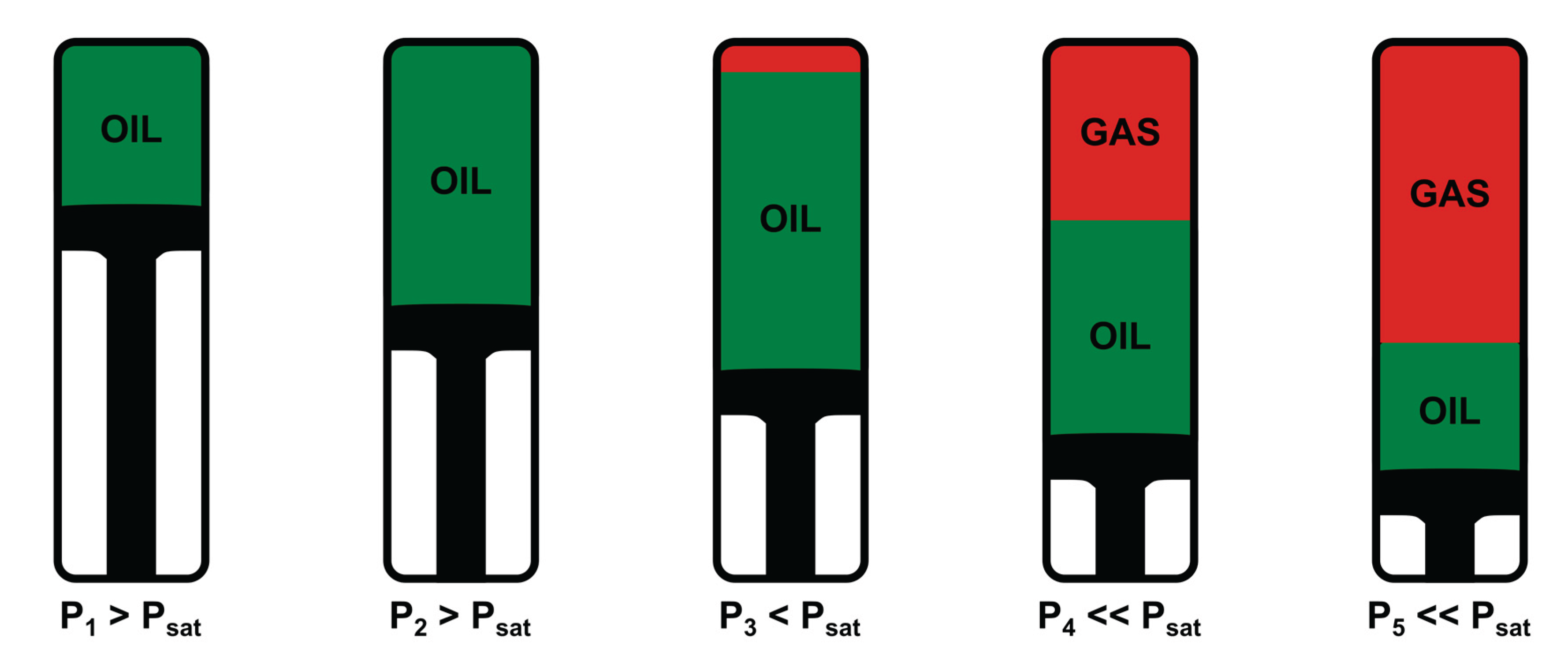
Figure 2.
The distribution of all archive fluids intra-distances (cyan) are compared to the distribution of the distances of a test fluid against the dBase (shown in orange). The selected closest neighbors distances are shown in dashed black lines.
Figure 2.
The distribution of all archive fluids intra-distances (cyan) are compared to the distribution of the distances of a test fluid against the dBase (shown in orange). The selected closest neighbors distances are shown in dashed black lines.
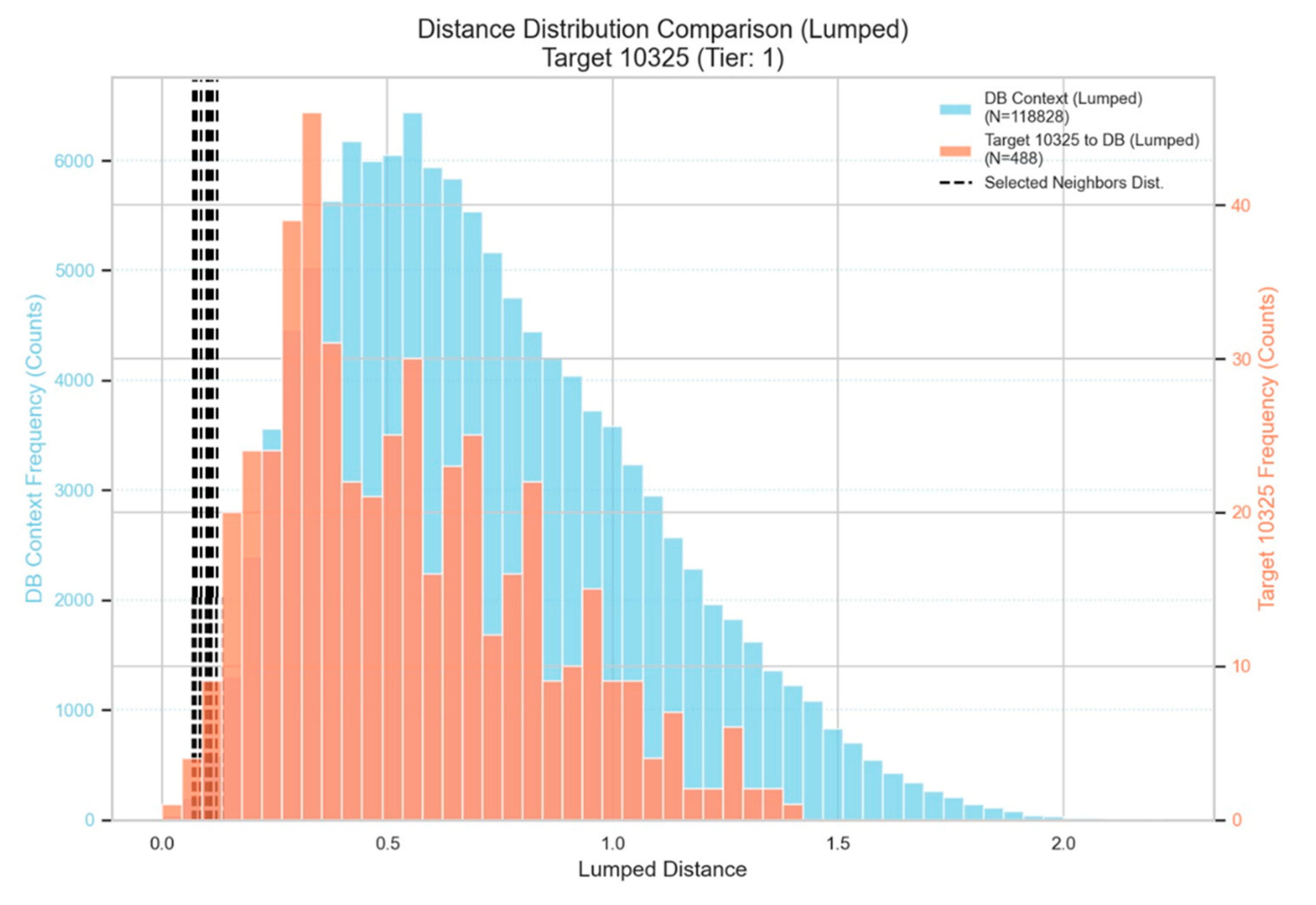
Figure 3.
Geometric interpretation of the Taylor step within the Local Interpolation Model (LIM). The method applies a simultaneous, vector-based correction in the input space defined by composition and temperature to estimate the PVT property of the test fluid from its neighbor.
Figure 3.
Geometric interpretation of the Taylor step within the Local Interpolation Model (LIM). The method applies a simultaneous, vector-based correction in the input space defined by composition and temperature to estimate the PVT property of the test fluid from its neighbor.
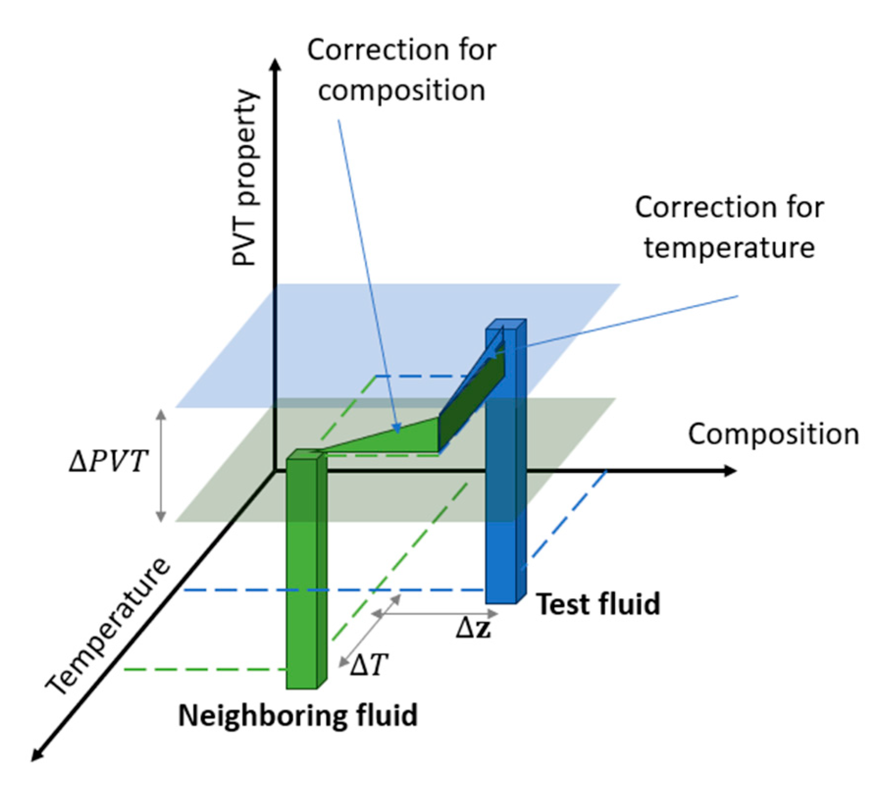
Figure 4.
Geometric interpretation of the Taylor step within the Local Interpolation Model (LIM). Left: Taylor-based correction from a neighboring fluid toward a test fluid using composition, temperature, and characterization differences. Right: Neighborhood structure in the trust region, where derivatives are shared and optimized across all pairwise connections.
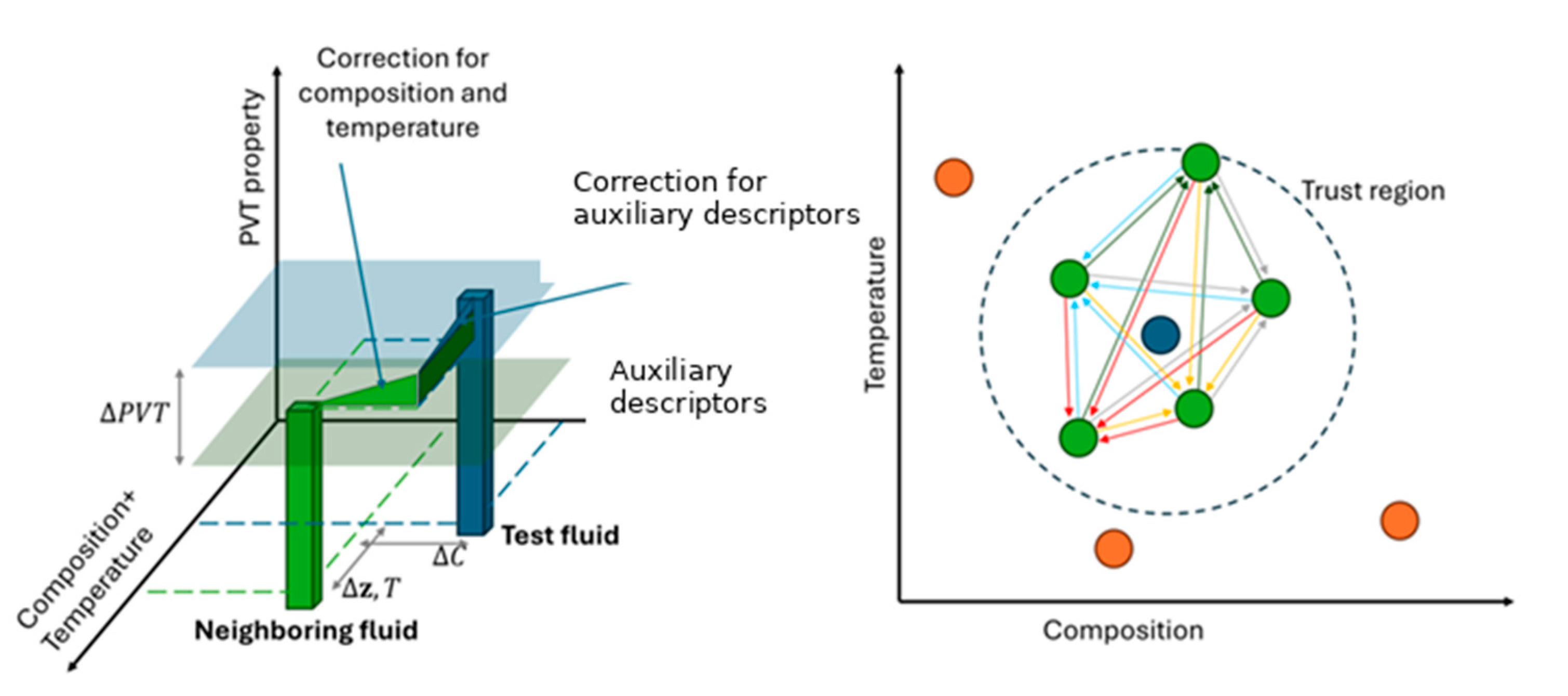
Figure 5.
PVT predictions workflow.
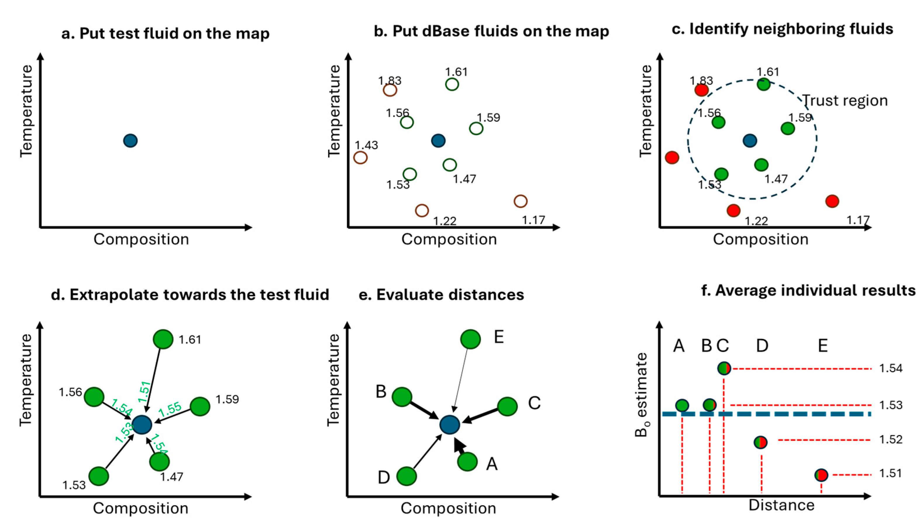
Figure 6.
Methodology to reconstruct the curve of a test fluid.
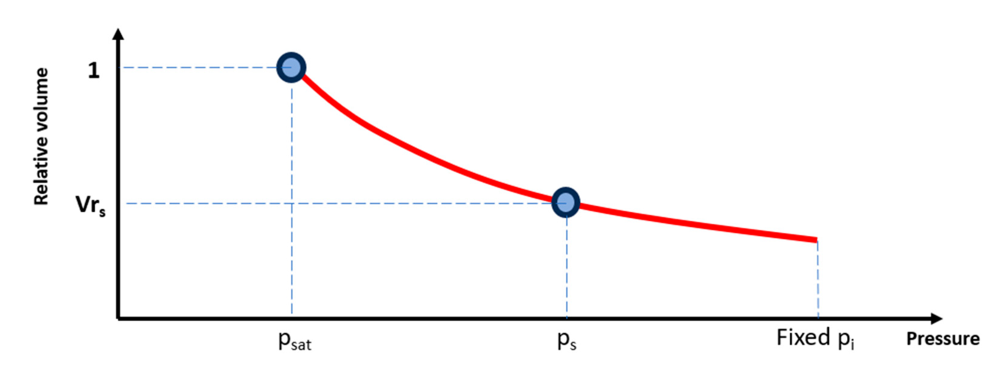
Figure 7.
Methodology to reconstruct the curve of a test fluid.
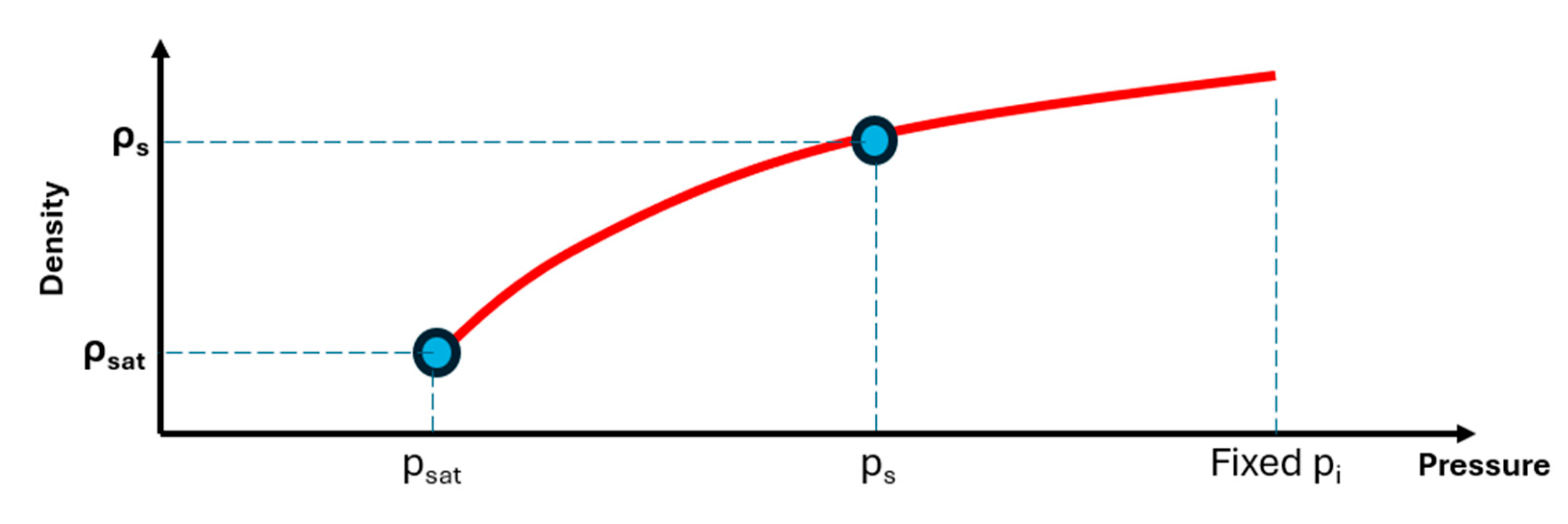
Figure 8.
Methodology to reconstruct the curve of a test fluid.
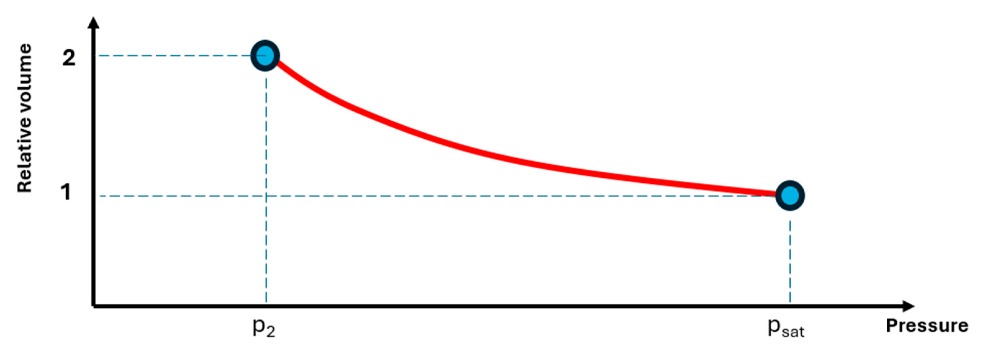
Figure 9.
Example inferred monophasic relative-volume curves.
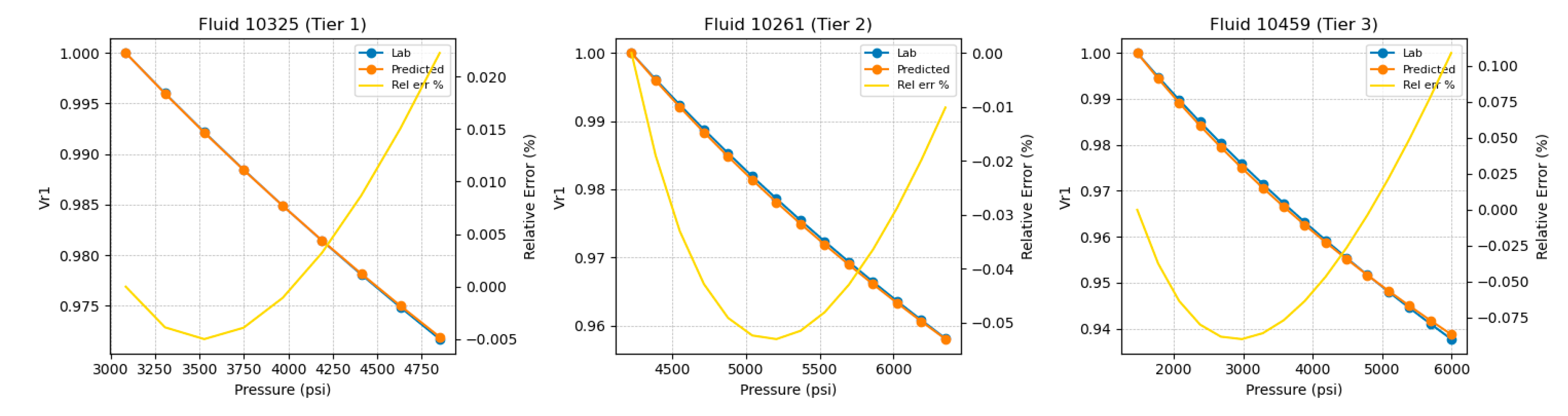
Figure 10.
Neighbors normalized curves identified by the tiering system.
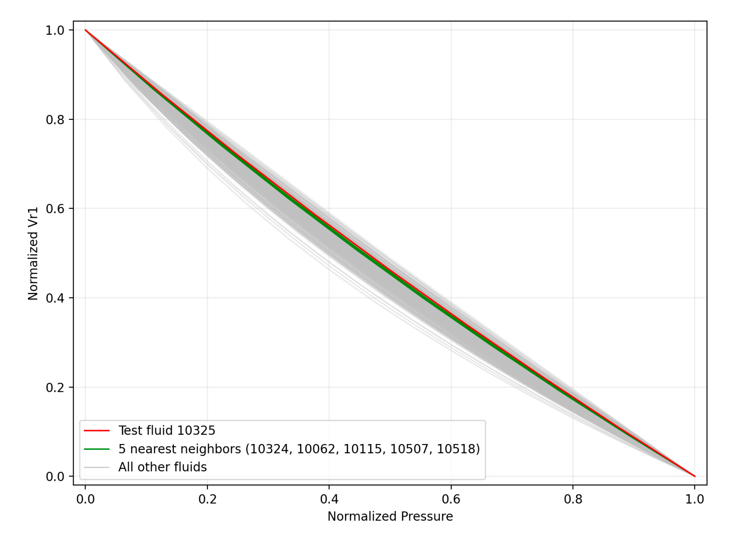
Figure 11.
Database-wide accuracy in predicted monophasic Vr1 curves.
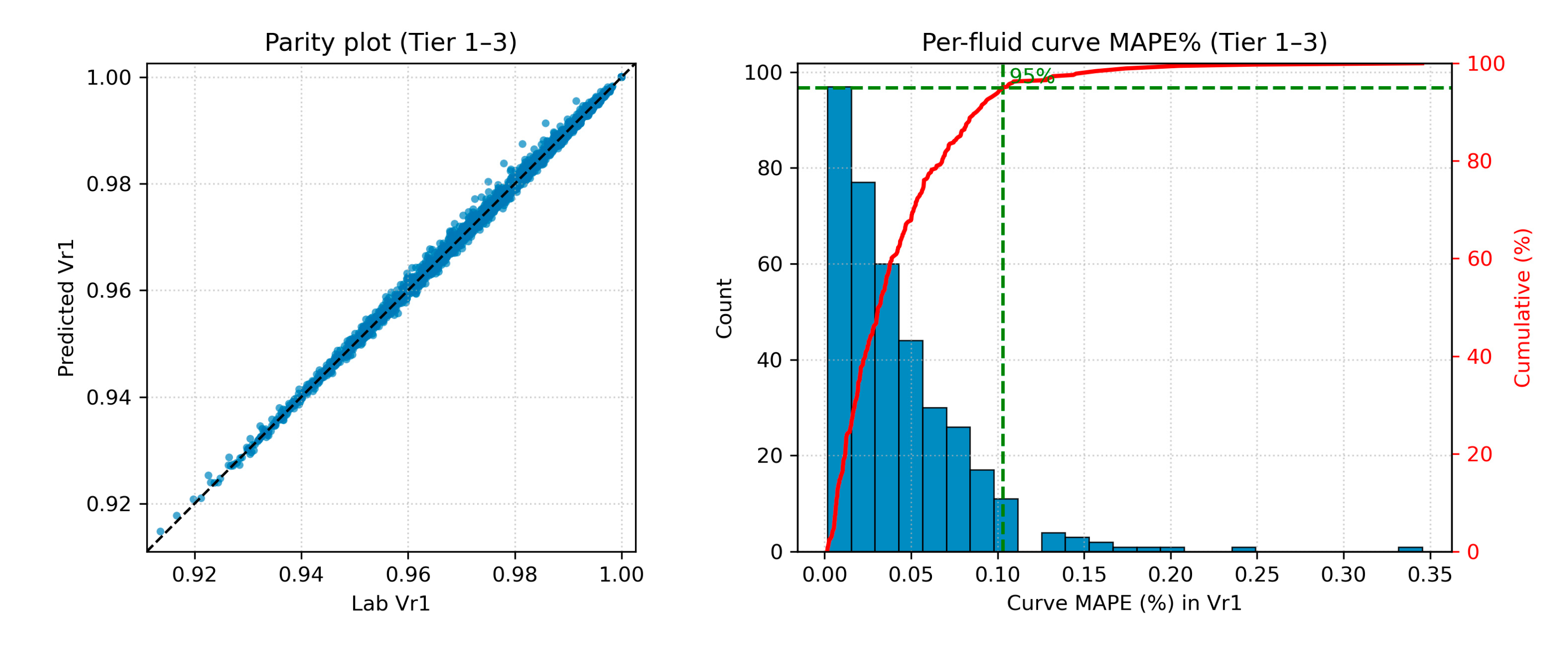
Figure 12.
Example inferred monophasic density curves.
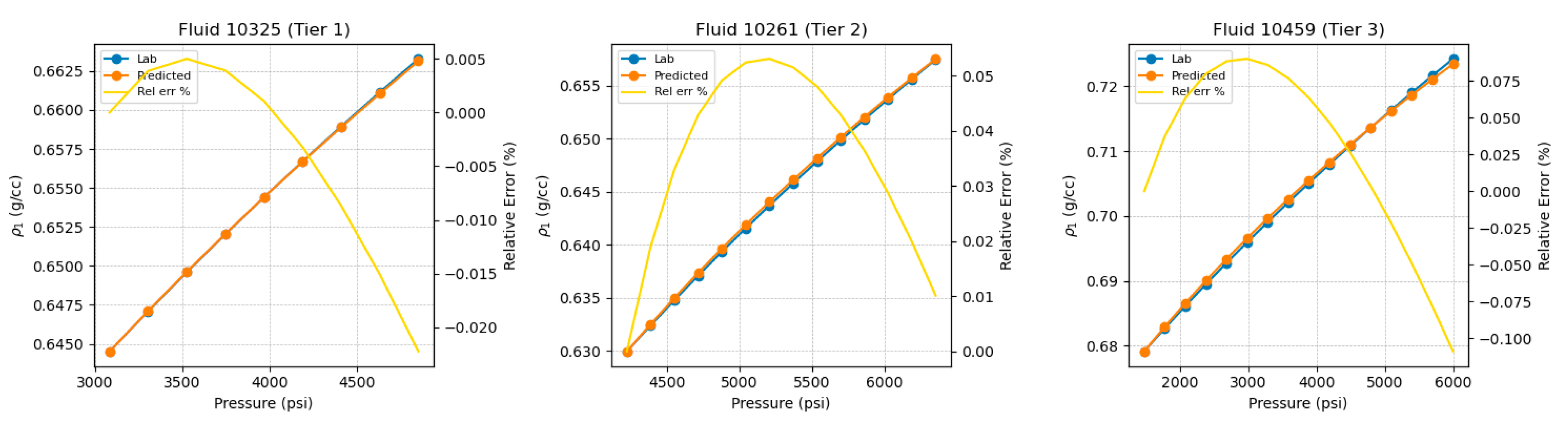
Figure 13.
Database-wide accuracy in predicted monophasic density curves.
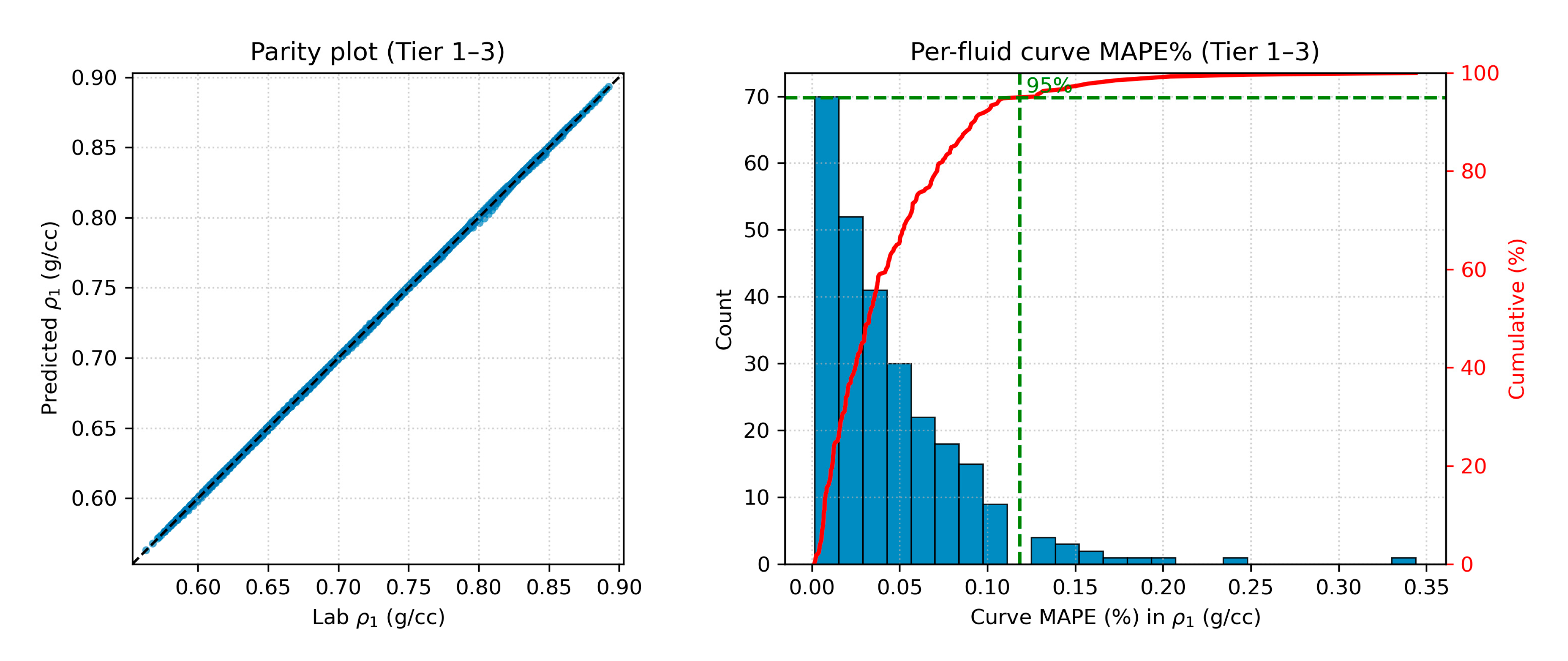
Figure 14.
Example inferred compressibility curves.
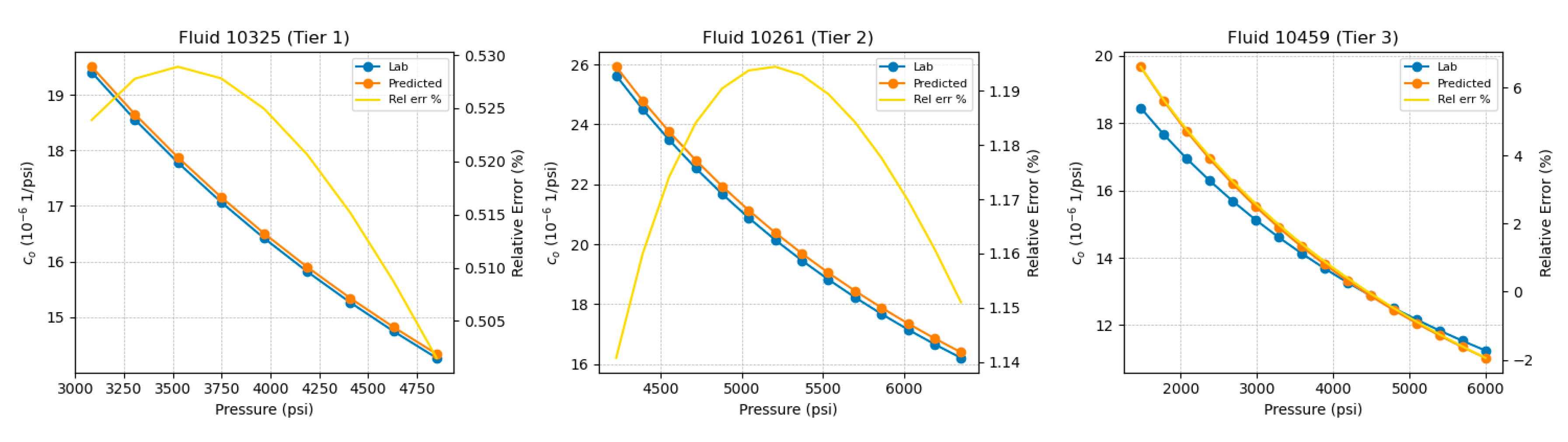
Figure 15.
Database-wide accuracy in predicted compressibility curves.
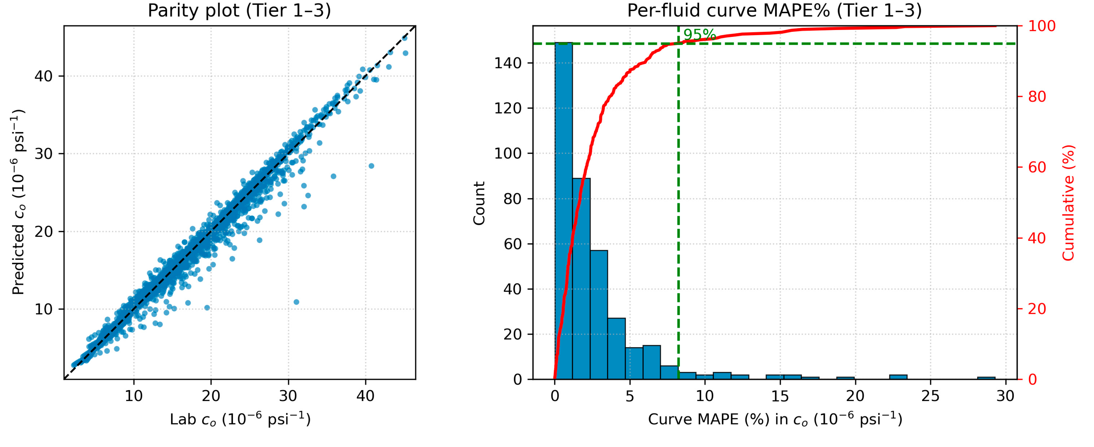
Figure 16.
Parity plot for P2.
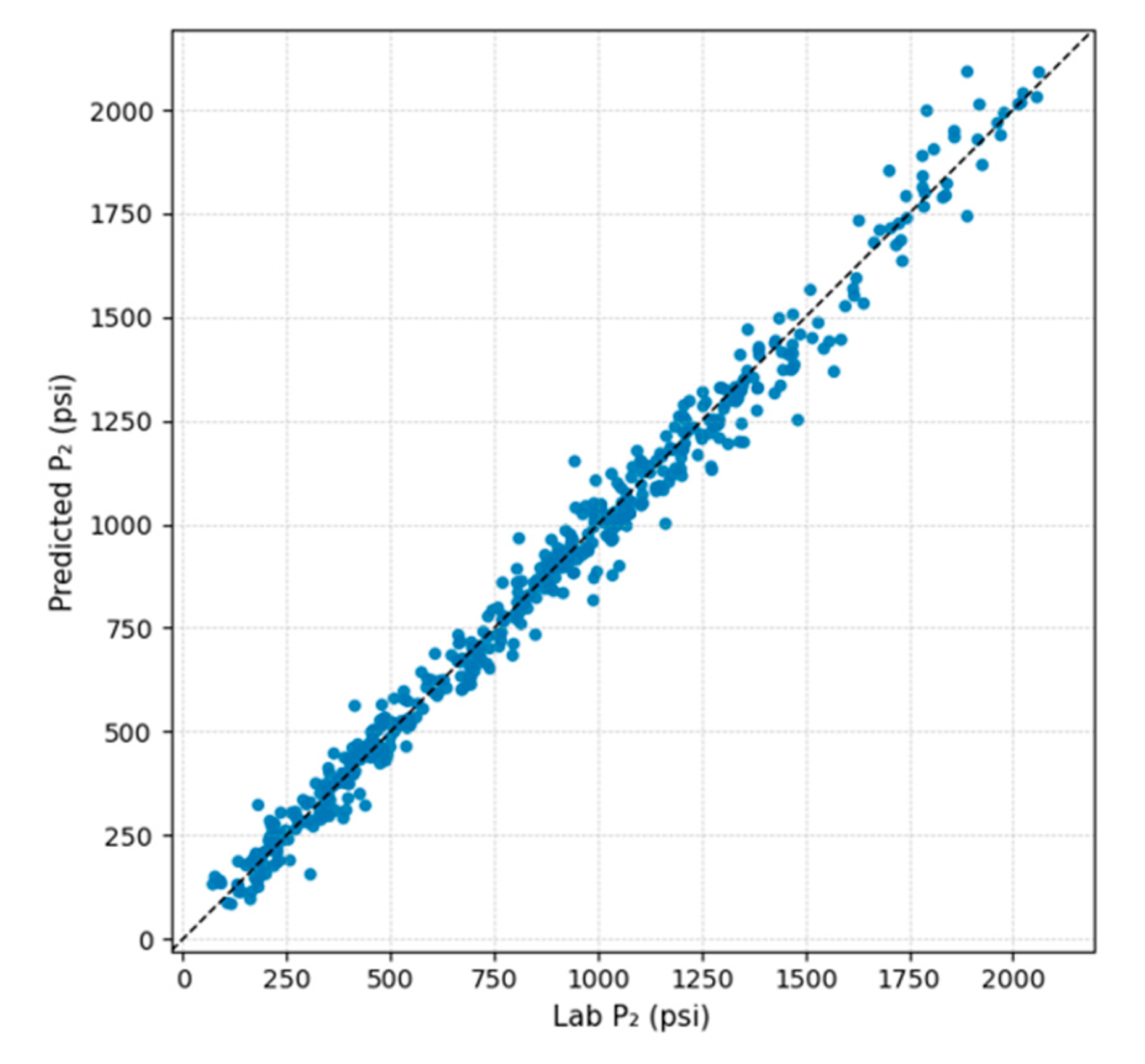
Figure 17.
Example inferred diphasic relative-volume curves.
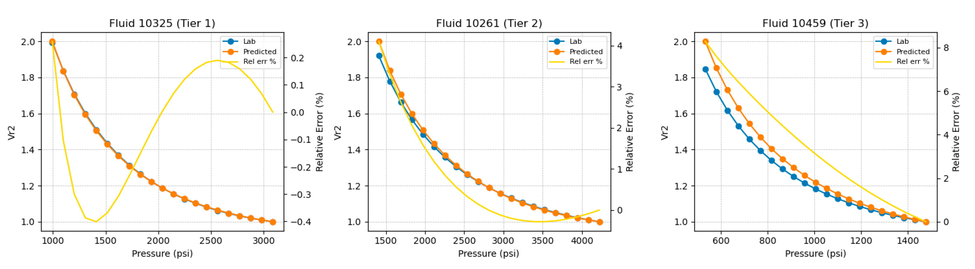
Figure 18.
Database-wide accuracy in predicted Vr2 curves.
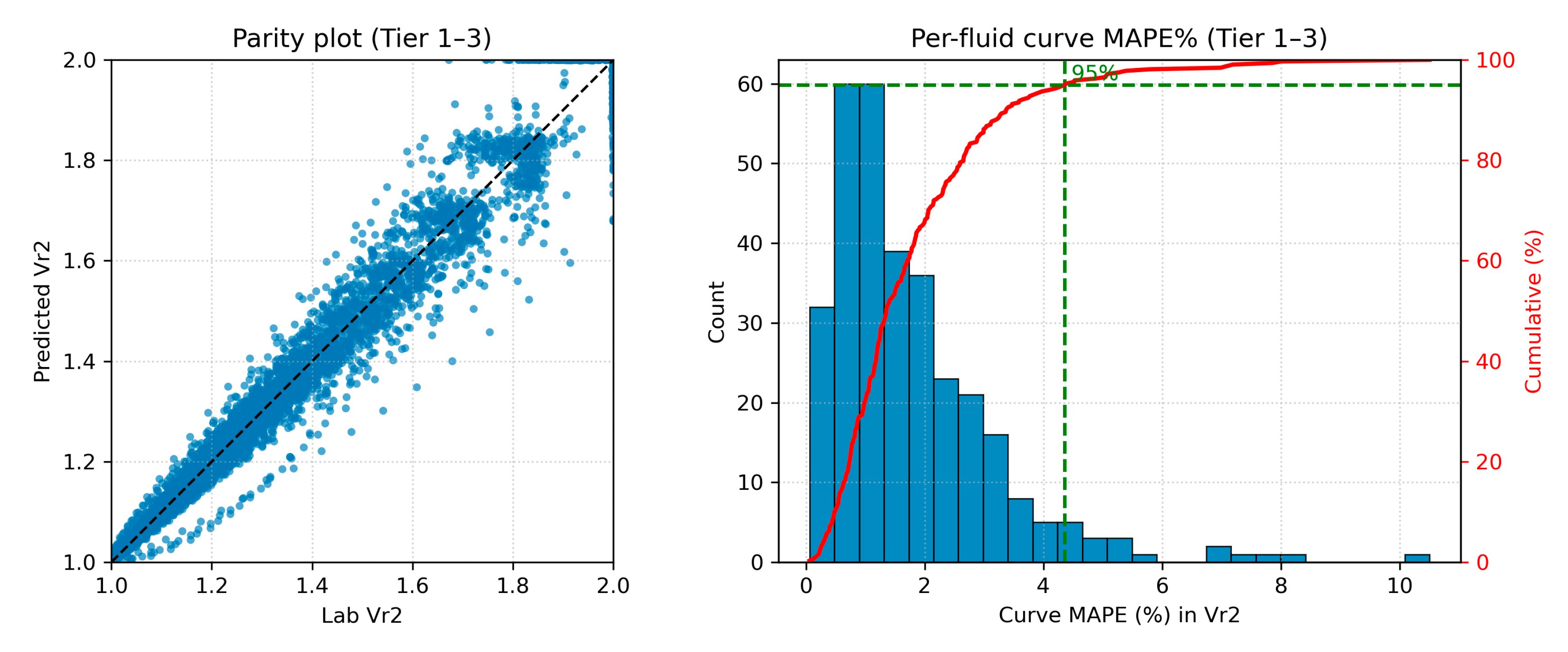
Figure 19.
Neighbors normalized curves identified by the tiering system.
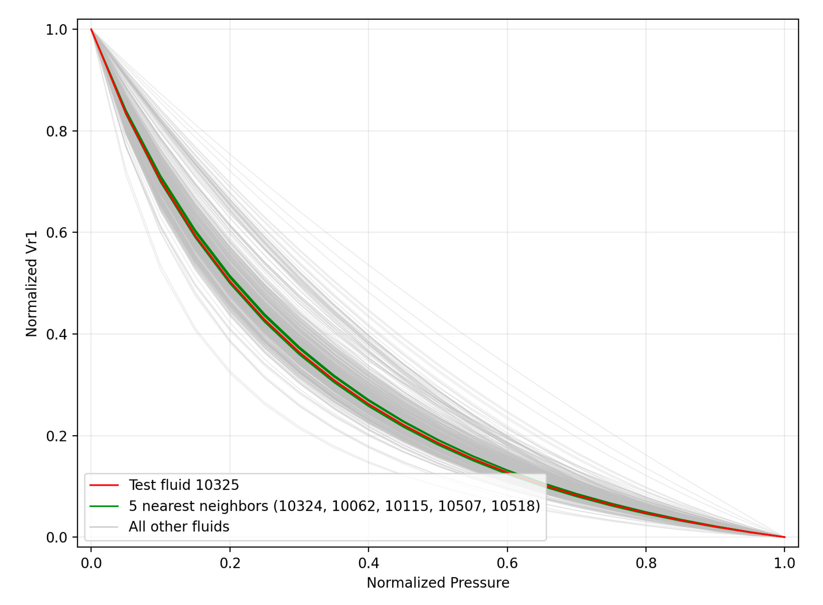

Table 1.
Tier-resolved error statistics for monophasic relative volume
| Tier | Size | Mean MAPE (%) | Std MAPE (%) |
| Overall (Tier 1-3) | 376 | 0.04 | 0.04 |
| Overall (Tier 1-6) | 488 | 0.07 | 0.10 |
| 1 | 248 | 0.04 | 0.04 |
| 2 | 97 | 0.05 | 0.04 |
| 3 | 31 | 0.04 | 0.04 |
| 4 | 23 | 0.07 | 0.08 |
| 5 | 29 | 0.09 | 0.1 |
| 6 | 60 | 0.21 | 0.20 |
Table 2.
Tier-resolved error statistics for monophasic density
| Tier | Size | Mean MAPE (%) | Std MAPE (%) |
| Overall (Tier 1-3) | 376 | 0.04 | 0.04 |
| Overall (Tier 1-6) | 488 | 0.07 | 0.11 |
| 1 | 248 | 0.04 | 0.04 |
| 2 | 97 | 0.05 | 0.05 |
| 3 | 31 | 0.04 | 0.04 |
| 4 | 23 | 0.08 | 0.09 |
| 5 | 29 | 0.10 | 0.11 |
| 6 | 60 | 0.32 | 0.25 |
Table 3.
Tier-resolved error statistics for compressibility
| Tier | Size | Mean MAPE (%) | Std MAPE (%) |
| Overall (Tier 1-3) | 376 | 2.65 | 3.17 |
| Overall (Tier 1-6) | 488 | 2.84 | 3.45 |
| 1 | 248 | 2.73 | 3.80 |
| 2 | 97 | 2.60 | 2.92 |
| 3 | 31 | 2.18 | 1.87 |
| 4 | 23 | 3.32 | 3.54 |
| 5 | 29 | 2.29 | 2.35 |
| 6 | 60 | 4.11 | 3.55 |
Table 4.
Tier-resolved error statistics for diphasic relative volume
| Tier | Size | Mean MAPE (%) | Std MAPE (%) |
| Overall (Tier 1-3) | 376 | 1.78 | 1.32 |
| Overall (Tier 1-6) | 488 | 1.89 | 1.55 |
| 1 | 248 | 1.74 | 1.39 |
| 2 | 97 | 1.73 | 1.20 |
| 3 | 31 | 2.27 | 2.09 |
| 4 | 23 | 2.19 | 1.69 |
| 5 | 29 | 2.26 | 1.85 |
| 6 | 60 | 2.26 | 2.00 |
Disclaimer/Publisher’s Note: The statements, opinions and data contained in all publications are solely those of the individual author(s) and contributor(s) and not of MDPI and/or the editor(s). MDPI and/or the editor(s) disclaim responsibility for any injury to people or property resulting from any ideas, methods, instructions or products referred to in the content. |
© 2026 by the authors. Licensee MDPI, Basel, Switzerland. This article is an open access article distributed under the terms and conditions of the Creative Commons Attribution (CC BY) license (http://creativecommons.org/licenses/by/4.0/).
Copyright: This open access article is published under a Creative Commons CC BY 4.0 license, which permit the free download, distribution, and reuse, provided that the author and preprint are cited in any reuse.


