
Submitted:
20 January 2026
Posted:
21 January 2026
You are already at the latest version
Abstract
Traffic forecasting in cellular networks is a challenging spatiotemporal prediction problem due to strong temporal dependencies, spatial heterogeneity across cells, and the need for scalability to large network deployments. Traditional cell-specific models incur prohibitive training and maintenance costs, while global models often fail to capture heterogeneous spatial dynamics. Recent spatiotemporal architectures based on attention or graph neural networks improve accuracy but introduce high computational overhead, limiting their applicability in large-scale or real-time settings. We propose HiSTM (Hierarchical SpatioTemporal Mamba), a spatiotemporal forecasting architecture built on state-space modeling. HiSTM combines spatial convolutional encoding for local neighborhood interactions with Mamba-based temporal modeling to capture long-range dependencies, followed by attention-based temporal aggregation for prediction. The hierarchical design enables representation learning with linear computational complexity in sequence length and supports both grid-based and correlation-defined spatial structures. Cluster-aware extensions incorporate spatial regime information to handle heterogeneous traffic patterns. Experimental evaluation on large-scale real-world cellular datasets shows that HiSTM achieves state-of-the-art accuracy, with up to 29.4% MAE reduction over strong spatiotemporal baselines and 47.3% improvement on unseen datasets. HiSTM shows improved robustness to missing data and better stability in long-horizon autoregressive forecasting, showcasing its effectiveness for scalable 5/6G traffic prediction.
Keywords:
time series forecasting
; spatiotemporal modeling
; 5G network traffic prediction
; deep learning
; state space models
; Mamba architecture
; attention mechanisms
; convolutional neural networks (CNNs)
; AI for telecommunications
1. Introduction
Accurate traffic forecasting is critical to predictive network resource allocation, network planning, and network optimization, directly influencing the operational expenditure of telecom providers [1]. Traditional time series forecasting methods such as ARIMA [2] and machine learning (ML) based models such as LSTM [3] treat each base station independently and fail to account for spatial dependencies among neighboring cells. To address this challenge, recent work has focused on employing ML-based models jointly with data pre-processing and feature engineering techniques to incorporate spatial knowledge in the training procedure [4,5].
A key challenge in spatiotemporal modeling is the trade-off between using a single global model and multiple cell-specific models. While cell-specific models can capture local dynamics with higher fidelity, they are costly to train, validate, deploy, and maintain, especially at the scale of modern cellular networks. In contrast, a global model is trained to cover the entire spatial grid. A global model incorporates spatial dependencies as features and formulates the forecasting task as a multivariate time series problem. Although global models can exploit shared patterns across cells, they often underperform due to distributional heterogeneity [1]. In 5G networks, user mobility and overlapping coverage introduce more complex spatial correlations [6], rendering purely temporal modeling insufficient, which leads to large forecasting errors.
By explicitly modeling spatial context alongside temporal dynamics, spatiotemporal architectures have the potential to mitigate the limitations of standalone temporal approaches. Indeed, a single spatiotemporal model could exploit correlations among neighboring cells, leading to higher forecasting accuracy. Recent advancements using graph neural networks (GNNs) and attention-based models have shown promise in learning complex spatiotemporal dependencies [7]. However, these architectures suffer from high computational cost, which limits the feasibility of their real-time large-scale deployment.
To address these challenges, we propose the Hierarchical SpatioTemporal Mamba (HiSTM), a novel spatiotemporal forecasting model based on the Mamba architecture [8] that employs a hierarchical design to capture both local variability and global patterns. HiSTM formulates cellular traffic forecasting as a multivariate time series over spatial frames, where each cell is treated as a pixel and its traffic measurements evolve over time. Frame-wise spatial encoding applies spatial convolutions independently at each time step to capture local neighborhood context, which is subsequently modeled using Mamba-based state-space dynamics for temporal forecasting. Unlike graph-based or attention-heavy models, the HiSTM achieves strong predictive accuracy while maintaining low computational overhead. It provides a favorable trade-off between performance and scalability.
Our main contributions are summarized as follows:
- We propose HiSTM, a hierarchical spatiotemporal forecasting architecture that performs frame-wise spatial encoding using CNNs, models temporal dynamics via Mamba state-space blocks, and aggregates temporal information through attention-based mechanisms.
- We show that HiSTM achieves state-of-the-art performance on the Milan cellular traffic dataset, reducing MAE by 29.4% compared to the STN baseline and achieving the lowest RMSE among all evaluated models. The model exhibits a strong cross-dataset generalization, achieving a 47.3% MAE improvement on the unseen Trentino dataset and successfully adapting to correlation-based network topologies (Liverpool 5G RU).
- We introduce cluster-aware variants (Global-Aware and ClusterFiLM) to explicitly model spatial heterogeneity. Our results show that a single Global-Aware HiSTM model outperforms 10,000 independently-trained LSTMs, demonstrating the advantage of learning shared representations of traffic regimes over localized training.
- We evaluate robustness under missing and noisy data conditions and show that HiSTM maintains stable performance with up to 30% data loss in comparison to baselines.
- We show that HiSTM provides improved long-horizon forecasting stability, exhibiting a 58% slower error accumulation rate compared to STN in autoregressive multi-step prediction.
This article substantially extends our previous conference work [9]. The description of the proposed model architecture and a section of the Milan evaluation are based on the conference version. However, this study goes significantly further by introducing: a bigger set of strong contemporary baselines, cluster-based models/experiments, benchmarking against 10,000 local LSTMs, correlation-based datasets, ablation/granularity studies, and explainability analyses.
The rest of this paper is structured as follows: Section II reviews 5G traffic prediction methods. Section III formalizes the forecasting problem and introduces HiSTM along with baseline models. Section IV describes the datasets and experimental setup. Section V presents results and analysis, including ablation studies and large-scale comparisons. Section VI provides an explainability analysis of the model’s internal dynamics. Section VII concludes the study and outlines directions for future work.
2. Related Work
Traditionally, 5G traffic forecasting is treated as a purely temporal forecasting task, relying on recurrent neural networks. AI-based models such as vanilla RNNs, LSTMs [3], and GRUs [10] were applied to learn sequential traffic patterns, often achieving gains over classical time-series methods such as ARIMA [2]. However, these approaches inherently ignore spatial correlations. Prior studies note that while RNN-based methods can capture long-term dependencies, they neglect spatial context, reducing their effectiveness [11,12]. For example, Chen et al. proposed a multivariate LSTM (MuLSTM) using dual streams for traffic and handover sequences, but the model remains fundamentally temporal [13].
Temporal models employ hybrid or preprocessing strategies for improved accuracy. For instance, Hachemi et al. [4] applied an FFT filter before LSTM to separate periodic signals, while Wang and Zhang [5] used Gaussian Process Regression alongside LSTM to manage bursty patterns. These methods often operate at hourly aggregation levels and improve accuracy in long-term forecasts. However, they still lack spatial awareness and suffer from high computational and memory costs, limiting their applicability in large-scale or real-time cellular deployments.
More recently, transformer-based architectures have gained traction for temporal sequence modeling due to their ability to capture global dependencies and adapt to irregular patterns. Models such as Informer [14], Autoformer [15], TimesNet [16], and PatchTST [17] achieve state-of-the-art results in long-sequence time-series forecasting. These methods introduce efficient attention mechanisms, decomposition blocks, and frequency-domain representations to handle non-stationary patterns and long-range dependencies. However, despite their performance gain in long-range temporal forecasting, they still treat traffic data as independent sequences and overlook spatial correlations among base stations.
Recently, spatial models have become popular as they can exploit spatial correlations within the data. For example, grid-based methods apply ConvLSTM [18] or 3D-CNNs to traffic maps [19], though these require regular cell layouts. Graph-based architectures, such as STCNet and its multi-component variant A-MCSTCNet, combine CNNs or GRUs with attention mechanisms [20]. STGCN-HO uses graph convolutions based on handover-derived adjacency to model spatial links across base stations, with Gated Linear Units (GLUs) for time dependencies [21]. Many of these models supplement deep networks with auxiliary features, such as weekday labels or slice-specific parameters, to improve generalization. More advanced spatiotemporal architectures, such as DSTL, adopt a dual-step transfer learning scheme that clusters gNodeBs and fine-tunes shared RNN models per group [22]. It forecasts at a 10-minute interval while reducing training overhead. Spatiotemporal models that incorporate spatial structure can capture richer dependencies, but this often comes with increased architectural complexity and computational cost. In prior work, we investigated an enhanced Spatiotemporal Network (STN) for cellular traffic forecasting that combines a temporal sLSTM branch (an xLSTM implementation [23]) with a Conv3D spatial branch and fuses both streams via attention-based integration [24]. Although the model achieved strong spatiotemporal forecasting accuracy and improved generalization to unseen regions, these gains came with a substantial computational footprint, including higher memory usage, increased MACs, larger model size, and elevated inference latency (especially at the grid level). Consequently, the approach can be incompatible with deployment scenarios that impose strict latency or resource constraints. This motivates our investigation of structured state-space and Mamba-based models for spatiotemporal forecasting, which aim to retain predictive quality while reducing computational overhead.
To the best of our knowledge, Mehrabian et al. [25] published the first model to incorporate the Mamba framework into a spatiotemporal graph-based predictor for 5G traffic. It adapts a dynamic graph structure within a bidirectional Mamba block to model complex spatial and temporal dependencies.
In contrast to graph-based Mamba predictors that operate on an explicit graph structure, HiSTM models spatiotemporal dynamics using kernelized neighborhood tensors. For grid datasets, a neighborhood centered kernel is extracted on each target cell (c.f. 4.3.1), while non-grid datasets, the neighborhoods are constructed by ranking other cells using Pearson correlation computed on the training interval (c.f. 4.3.2). This design avoids reliance on a predefined graph while retaining spatial context in a consistent tensor form.
Despite recent advances, existing spatiotemporal forecasting models face a fundamental trade-off between modeling capacity and scalability. Attention- and graph-based architectures capture complex dependencies but incur high computational overhead, while simpler models fail to account for spatial heterogeneity. This gap motivates the need for a scalable spatiotemporal architecture that jointly models spatial and temporal dependencies without relying on expensive attention mechanisms or explicit graph construction.
In contrast, our model, HiSTM, uses the Mamba framework and adapts data input and output processing to work directly on spatial grids with temporal attention layers. This design improves accuracy and efficiency, especially for long-term forecasts and generalization to unseen data. Accordingly, we evaluate HiSTM against strong representatives of temporal Transformers, recurrent spatiotemporal predictors, and modern sequence backbones (c.f. 4.2) under a unified experimental protocol.
3. System Design
This section formalizes the spatiotemporal forecasting problem and describes the proposed model architectures.
3.1. Problem Formulation
Cellular network traffic forecasting aims to predict future traffic volume based on historical observations. We formulate this task as a spatiotemporal sequence prediction problem. Given a sequence of traffic measurements where each represents a spatial grid of cells at time step t, our goal is to predict the next traffic volume grid .
Beyond grid-structured maps, the same formulation can be applied by constructing semantic neighborhood tensors; in this paper we instantiate this by defining neighborhoods using Pearson correlation computed on the training interval and arranging the top-correlated cells into a kernel. Each grid cell contains a scalar value representing the traffic volume. This volume correlates with resource demands in the cellular network.
We define our input tensor as , where T is the sequence length (window of observation time steps), represents the spatial dimensions of the input kernel, and are the spatial coordinate in the grid . The prediction target is ,
representing the traffic volume at the center cell of the kernel for the next time step. Formally, we aim to learn a function that minimizes the prediction error , where L is the loss function (i.e., Mean Absolute Error), and represents the learnable parameters of the model. The spatiotemporal nature of the data introduces a unique challenge: capturing both spatial correlations between neighboring cells and temporal dependencies across the sequence.
3.2. Proposed Architecture: HiSTM
We propose the Hierarchical SpatioTemporal Mamba (HiSTM), an architecture that combines hierarchical spatiotemporal processing with attention-based temporal aggregation (Figure 1). The term "hierarchical" here refers to the progressive abstraction of features: starting from raw local spatial interactions (Convolution), to temporal dynamics (Mamba), and finally aggregating into a high-level global context (Attention). Given an input tensor (where T is the number of time steps and is the spatial kernel), the model predicts target values through three key components.
3.2.1. Hierarchical Spatiotemporal Encoding
The input is first augmented with an initial channel dimension (i.e., ), then passes through N stacked Encoder Layers. Each Encoder Layer l transforms its input (where is the initial augmented input) into an output . The operations within each layer are:
- Spatial Convolution: Input features are first reshaped appropriately (e.g., to ). A 2D convolution followed by a ReLU activation is applied. The first layer up-projects to C channels. Subsequent layers take channels and output C channels.
- Temporal Mamba Processing: The C-channel output from the convolution is reshaped to . A Mamba SSM [8] then models the temporal dependencies for each of the spatial locations treated as sequences of length T, with .
We use Mamba for its state space foundation, which models sequences through continuous-time dynamics rather than attention. This enables precise control over temporal structure and inductive bias, making it suitable for forecasting tasks where long-range temporal dependencies interact with fine-grained spatial patterns. Its ability to selectively retain and propagate information aligns with the demands of spatiotemporal modeling.
The Mamba output is reshaped back to , forming . The output of this encoding stage is .
3.2.2. Temporal Attention-Based Aggregation
From the encoded features , features corresponding to the center spatial cell are extracted across all T time steps. This yields a sequence . An attention mechanism then computes an aggregated context vector :
where is the feature vector from (for a given batch instance) at time step t. The layer maps from , producing a scalar energy . The softmax function normalizes these energies across all T time steps to obtain attention weights .
3.2.3. Prediction Head
Finally, the aggregated context vector is fed into a Multilayer Perceptron (MLP) head. This MLP consists of two linear layers with a ReLU activation in between, passing the dimensionality from C to , and then to 1, to produce the final prediction .
3.2.4. Cluster-Aware Variants
To investigate the impact of spatial heterogeneity on model performance, we introduce two cluster-aware extensions to the base HiSTM architecture. These variants leverage external knowledge about traffic regimes (e.g., Urban vs. Rural) during training:
- Global-Blind (GB):
- A single HiSTM model trained on all regions, but without any explicit cluster identifier. This setup ignores spatial heterogeneity and serves as a global baseline.
- Global-Aware (GA):
- This variant incorporates a learnable cluster embedding associated with the cluster label c of the target cell. The embedding is added to the feature representation before the final MLP head, enabling the model to condition its predictions on region-specific characteristics.
- Cluster-Specific (CS):
- Four separate HiSTM models are trained, one for each spatial cluster, using only data belonging to that cluster. This configuration represents cluster-localized learning without any information sharing across regions.
- ClusterFiLM (CF):
- This variant employs Feature-wise Linear Modulation (FiLM) [26]. A FiLM generator network takes the cluster label c as input and produces scaling () and shifting () parameters, which modulate intermediate feature maps in the encoder layers via an affine transformation:
This mechanism allows the model to dynamically adapt its internal representations based on spatial context.
In addition, we consider CF-Unbalanced, a variant of ClusterFiLM trained with a cluster-weighted loss to compensate for data imbalance across regions.
4. Datasets & Experimental Setup
This section outlines the datasets, preprocessing steps, training configuration, and evaluation process used to assess model performance in spatiotemporal data forecasting.
4.1. Datasets
We utilize two distinct datasets to evaluate HiSTM’s performance across different spatial topologies: geospatial grid and correlation-based (relational network) data.
4.1.1. Geospatial Data (Milan and Trentino)
Introduced by Barlacchi et al. [27], this dataset represents a classic Euclidean topology where traffic is aggregated into a regular spatial grid ( for Milan, for Trentino). Spatial dependencies are inherently geometric; the "neighbors" of a cell are its physically adjacent grid cells. The data exhibits significant spatial heterogeneity (Figure 2), with activity concentrated in urban centers and dispersed in rural peripheries. Traffic is sampled at 10-minute intervals (144 measurements per day).
Lag plot analysis (Figure 3) reveals that these datasets maintain correlation at higher lag values. Individual cell traffic demonstrates higher volatility (Approximate Entropy [28] of 1.386 for a single cell) compared to spatially aggregated traffic (0.196), with the latter exhibiting enhanced cyclical patterns and passing the Augmented Dickey Fuller test [29] for stationarity. It is evident that the aggregated series is more correlated with itself for different lags; hence, it is easier to predict. Consequently, incorporating the spatial element in the prediction can help the model to capture the distribution more effectively, reduce the influence of individual events, and magnify predictable cyclical patterns.
To characterize spatial heterogeneity in traffic patterns, we partition the study area into four spatial clusters using mean traffic volume computed on the training set. This avoids information leakage from the evaluation period. The resulting clusters correspond to Downtown, Urban, Suburban, and Rural regions, exhibiting distinct traffic distributions and temporal dynamics (Table 1).
We characterize the temporal behavior within these spatial regions by comparing traffic distributions under different temporal conditions. We define nighttime as 22:00–06:00 and daytime as 06:00–22:00. Figure 4 shows a diurnal separation across all spatial types, with reduced volumes at night. The effect is strongest in Downtown, while Suburban and Rural areas show comparatively tighter distributions.
Figure 5 highlights a secondary weekly-cycle effect: activity decreases on weekends across all clusters, with the strongest shift in Downtown and comparatively stable behavior in Rural regions.
These spatial clusters are used in the cluster-aware HiSTM evaluation in 5.4.
4.1.2. Correlation-Based Relational Data (Liverpool 5G RU)
The Liverpool City Region High Density Demand (LCR HDD) project [30] tracks performance metrics at the Radio Unit (RU) level for high-density event venues (Salt & Tar and ACC Arena). Traffic is sampled at 1 second in Salt & Tar for 3,000 users and every 3 seconds in ACC Arena for 12,000 users, for a total of 10,000 timestamps. Unlike the grid-based Milan dataset, the "spatial" dependencies here are not defined by geometric proximity on a map, but by functional relationships (e.g., user load balancing, interference, and shared user mobility). This dataset challenges the model to capture dependencies in a graph-like structure where the "neighbors" are RUs with correlated traffic patterns, regardless of their physical distance.
4.2. Baseline Models
To assess the performance of our approach, we compare HiSTM with selected baselines that span a representative range of spatiotemporal forecasting paradigms, including convolutional models, recurrent architectures, Transformer-based methods, and state-space–inspired hybrids. These baselines cover models that emphasize spatial–temporal dependency modeling, long-range temporal dynamics, or computational efficiency in large-scale forecasting settings.
To assess the impact of cluster-aware conditioning, we compare HiSTM against two additional baseline configurations. Global-Blind (GB) refers to the standard HiSTM trained on the full dataset without cluster information, while Cluster-Specific (CS) consists of separate HiSTM models trained independently on data from each spatial cluster. These baselines allow us to isolate the effect of shared representation learning and explicit spatial conditioning.
Unless a baseline’s formulation restricts inputs, we train all models on the same forecasting task with identical temporal and spatial inputs: for each target cell, the input is a length-T history of neighborhoods and the target is the next-step value of the center cell. For the RU dataset, neighborhoods are constructed by correlation and provided in the same tensorized form. For purely temporal models (e.g., xLSTM), the spatial dimension is flattened to match the model’s expected input shape. Baseline architectures are configured following their original implementations, with hyperparameters selected to balance performance and computational efficiency. All models are trained under the same optimization and early-stopping criteria.
- Informer [14]: A Transformer variant utilizing the ProbSparse self-attention mechanism to efficiently handle long sequence forecasting with reduced computational overhead.
- AutoFormer [15]: An auto-correlation-based Transformer that decomposes time series into trend and seasonal components to improve long-term forecasting accuracy.
- TimesNet [16]: A unified temporal convolutional architecture that models multi-periodic patterns through 2D time–frequency representations, achieving strong results across various forecasting tasks.
- PatchTST [17]: A patch-based Transformer for time series forecasting that tokenizes continuous temporal segments into patches, enabling efficient long-sequence modeling.
- STN [19]: A deep neural network capturing spatiotemporal correlations for long-term mobile traffic forecasting.
- xLSTM [23]: A scalable LSTM variant with exponential gating and novel memory structures (sLSTM/mLSTM) designed as Transformer alternatives. For fair comparison, our implementation uses only one mLSTM layer (denoted as xLSTM[1:0] in their paper) to prioritize computational efficiency while retaining its parallelizable architecture.
- STTRE [31]: A Transformer-based architecture leveraging relative embeddings to model dependencies in multivariate time series.
- VMRNN-B & VMRNN-D [32]: Vision Mamba-LSTM hybrids addressing CNN’s limited receptive fields and ViT’s computational costs. VMRNN-B (basic) and VMRNN-D (deep) use Mamba’s selective state-space mechanisms for compact yet competitive performance.
- PredRNN++ [33]: An improved version of PredRNN that introduces gradient highway units and spatiotemporal memory flow to better capture long-term dependencies in sequence forecasting.
4.3. Data Preprocessing
To ensure robust spatiotemporal feature extraction, we apply different preprocessing strategies tailored to the topology of each dataset. For each prediction target , we construct the input by stacking the T most recent observations () of the cell’s neighborhood, i.e., we use a length-T sequence of past frames to forecast the next step. Depending on the dataset, the neighborhood is defined geospatially or semantically. Unless stated otherwise, all the model are trained as a spatiotemporal univariate timeseries, where the model has visibility to the target variable for T length and a frame.
4.3.1. Geospatial Grid Processing
For the grid-based Milan dataset, we preserve the inherent grid structure. We set a spatial kernel size of , exploiting the physical adjacency of cells. Boundary effects are mitigated by cropping the grid to , ensuring divisibility by the stride. Temporal sequences are constructed by concatenating six consecutive time steps ().
4.3.2. Correlation-Based Spatial Construction
For the RU dataset, which lacks a grid topology, we reconstruct a semantic spatial neighborhood to bridge the gap between correlation-based relationships and our kernel-based architecture. We define "spatial" proximity using Pearson correlation. For each target RU, we compute its temporal correlation with all other RUs and then construct a virtual spatial kernel where:
- The center pixel is the target RU itself.
- The surrounding pixels are populated by the top-correlated RUs, sorted by correlation strength (filling the inner ring first, then the outer ring).
This transformation allows the layers of spatiotemporal models to operate on "functional neighbors" (units that behave similarly) just as they would on physical neighbors.
4.3.3. Normalization and Splitting
For all datasets, inputs and targets are normalized to the [0, 1] range via Min-Max scaling fitted on the training set to prevent leakage. The data is chronologically partitioned into training (70%), validation (15%), and test (15%) sets.
4.4. Implementation and Training Configuration
We implement the HiSTM model in PyTorch, leveraging GPU-optimized operations for its Mamba and Conv2D modules to ensure computational efficiency. For reproducability, we release the complete source code for our HiSTM implementation in a public repository [34].
For training and inference, we use an AI-server with a single NVIDIA A100 80GB GPU with 64 CPU cores and 512 GB RAM, using CUDA 12.4 and PyTorch 2.6.0+cu124. All models are trained under the same optimization setup (Adam, learning rate , learning-rate scheduler, batch size 128) and the same early-stopping criterion (patience 15 with best checkpoint selected by validation loss).
4.5. Evaluation Metrics
We evaluate prediction accuracy using five metrics. Mean Absolute Error (MAE) measures the average absolute difference between predictions and ground truth, providing a straightforward assessment of overall accuracy. Root Mean Squared Error (RMSE) penalizes larger deviations more heavily, emphasizing sensitivity to outliers. The coefficient of determination (R²) quantifies the proportion of variance explained by the model, reflecting its explanatory power. Structural Similarity Index (SSIM) evaluates the spatial coherence and perceptual similarity of predicted traffic maps. In addition, Mean Absolute Percentage Error (MAPE) and Mean Average Scaled Error (MASE) are employed in the cell-level analysis to quantify relative accuracy across regions with varying traffic volumes. their percentage- and scaled-based interpretation is used for comparing model behavior between urban, suburban, and rural cells, where absolute traffic magnitudes differ in magnitude.
All metrics are computed after reversing the normalization to the original scale.
5. Results and Analysis
This section evaluates forecasting accuracy, cross-dataset generalization, robustness under missing observations, transfer to non-grid network topologies, and computational efficiency, comparing our proposed HiSTM model against the baselines.
To make the evaluation easier to follow, we organize the results from core predictive performance to increasingly deployment-relevant considerations. We first report single-step and autoregressive multi-step accuracy. We then evaluate cross-dataset generalization and robustness under controlled missing-data scenarios. Next, we test whether HiSTM transfers beyond grid-based traffic forecasting by using correlation-defined network neighborhoods on a 5G Radio Unit (RU) dataset. Finally, we analyze spatial heterogeneity via cluster-aware variants, contrast HiSTM with a large collection of independent local models, study architectural granularity (spatial kernel size and temporal look-back), and report computational efficiency.
Evaluation protocol. Unless otherwise stated, metrics are computed on the test set and averaged across all spatial locations (for sequence metrics: across test time indices). For multi-step forecasting, we use autoregressive rollout and report per-horizon averages. Best values within each table are highlighted in bold.
5.1. Prediction Accuracy
This subsection quantifies predictive performance under standard (non-cluster-aware) training, focusing on (i) single-step accuracy on Milan, (ii) multi-step autoregressive stability (error accumulation), and (iii) cross-dataset generalization to Trentino (unseen, yet similar, dataset).
5.1.1. Single-Step Prediction Results
On the Milan dataset, under the standard setting without cluster conditioning, HiSTM achieves the best single-step forecasting performance in terms of MAE and provides competitive improvements across complementary metrics (Table 2). The model attains the lowest RMSE and the highest score among the compared methods. The combination of frame-wise spatial encoding with Mamba-based temporal modeling yields strong next-step accuracy while preserving spatial structure.
5.1.2. Multi-Step Autoregressive Forecasting
Having established single-step accuracy, we evaluate the stability of HiSTM under autoregressive forecasting (multi-step on Milan dataset), where error accumulation poses a greater challenge. Due to the increased computational cost of autoregressive rollout, these experiments are conducted on a randomly sampled 20% subset of the test data. As this subset differs from the full test set used for single-step prediction, the first-step autoregressive results are not directly comparable to single-step scores. The same subset is used across all models, ensuring a fair and consistent comparison between the models in this evaluation.
HiSTM demonstrates improved stability over extended forecasting horizons (Table 3). While all models accumulate error as the forecast horizon increases, HiSTM maintains the lowest MAE and RMSE at each of the six temporal steps indicating improved temporal stability under autoregressive rollout. At step 6, HiSTM achieves an MAE that is 36.8% lower than STN and 11.3% lower than STTRE. The increasing performance gap under autoregressive rollout suggests that HiSTM accumulates less compounding error over multiple steps.
5.1.3. Cross-Dataset Generalization on Trentino Dataset
To assess whether the observed performance extends beyond the training distribution, we evaluate all models on the unseen Trentino dataset.
On the Trentino dataset, HiSTM achieves strong out-of-distribution performance (Table 4). Relative to STN, HiSTM reduces MAE by 47.3% and reduces RMSE by 36.9%. HiSTM also attains the highest SSIM and the highest score. In terms of RMSE, TimesNet scores lower (4.7210 vs. 4.8134), while HiSTM remains best on MAE and ties or leads on the other reported metrics. Overall, HiSTM exhibits a strong generalization capability to new spatial environments with different activity distributions and scales.
5.1.4. Cell-Specific Modeling and Spatially-Aware Accuracy
While aggregate metrics quantify average performance, they obfuscate local behavior; therefore, we examine cell-level forecasts to assess spatially-aware accuracy across representative traffic regimes.
We select a 7-day window (1008 time steps) from the Milan test set and generate one-step-ahead forecasts using a 6-step temporal memory window and an spatial kernel on the grid. To highlight spatial heterogeneity, we inspect four representative cells corresponding to (a) urban, (b) suburban, (c) rural, and (d) the cell with the maximum temporal variance (Figure 6). Predicted versus actual trajectories are shown in Figure 7.
The urban cell exhibits the lowest MAPE (8.49%), with close alignment between predicted and true trajectories even during peak periods. Performance remains stable in the suburban cell (11.62% MAPE). As expected, relative error increases in the rural cell (24.86% MAPE), where low absolute volumes can inflate percentage-based metrics. The high-variance cell remains challenging but is tracked reasonably well (15.30% MAPE), suggesting that HiSTM can handle non-stationary dynamics, with residual underestimation around sharp peaks indicating headroom for improving extreme-event modeling.
5.2. Missing Data
Next, We evaluate robustness to incomplete telemetry by injecting controlled missing values and imputing with last observation carried forward (LOCF) prior to forecasting. Table 5 reports MAE/RMSE across combinations of missingness in training and testing, isolating how performance degrades under increasing observation loss.
We synthetically introduce missing values into the Milan traffic frames , where denotes the scalar traffic value at spatial location at time t. Missingness is injected at the cell–time granularity, i.e., individual spatiotemporal entries . For each dataset split S with temporal length , we treat every spatial location independently as a univariate time series
Given a target missing-data rate (0%, 10%, 20%, and 30%), we partition the missing budget into two components intended to reflect common operational failure modes: random noise dropouts and contiguous outages. Specifically, of the missing values are assigned to random dropouts and to outages, yielding per-series counts and , respectively.
For the random-dropout component, we uniformly sample without replacement an index set with and set for all . For the outage component, we simulate contiguous telemetry losses by masking disjoint time intervals. Each interval is generated by sampling a start time and a duration
where T denotes the model lookback (sequence) length used to construct inputs. This choice enforces that any single outage spans at most two consecutive input windows. Intervals that overlap previously masked indices are rejected, and the procedure is repeated until exactly additional time steps are removed. The resulting outage index set can be written as
Missing patterns are generated independently for each spatial location , i.e., missingness is not correlated across space, and they are generated separately within each dataset split to avoid temporal leakage. The validation split remains uncorrupted.
After masking, we apply LOCF imputation independently along time for each , replacing every missing value with the most recent previously observed value in the same series. Because the first index of each split () is never masked, LOCF is always well-defined. Model inputs are then constructed from the imputed frames using the same temporal window length T and spatial kernel size K as in the main experimental setup.
We report MAE and RMSE over combinations of training and test missing-data conditions. Models are trained with 0% and 10% missing data and evaluated on test sets with 0–30% missing data. As shown in Table 5, HiSTM consistently achieves the best performance across all evaluated train/test combinations. When trained on complete data, HiSTM yields the lowest MAE and RMSE across test missing-data rates (MAE 5.1462–5.1451; RMSE 10.9949–10.9915), outperforming the next-best baseline (Informer). When trained with 10% missing data, HiSTM maintains its advantage (MAE 5.1762–5.1754) under all tested test-set missing-data levels.
Finally, we note that LOCF imputation can smooth short-term fluctuations; consequently, increasing the proportion of missing data may occasionally reduce apparent error for some methods by attenuating high-frequency variance in the inputs. The consistent ranking across all configurations nevertheless indicates that HiSTM is comparatively robust when operating on imputed streams, which reflects realistic deployment scenarios involving telemetry dropouts and temporary backhaul failures.
5.3. Performance on 5G High Density Demand (RU) Dataset
To test transfer beyond gridded maps, we evaluate all models on a non-grid 5G RU dataset where spatial neighborhoods are defined by correlation rather than physical adjacency. We report MAE per Key Performance Indicator (KPI) to assess whether HiSTM retains advantages under heterogeneous targets and graph-like dependencies.
We evaluate HiSTM on the Liverpool 5G High Density Demand dataset to assess its capability in forecasting complex network metrics beyond traffic volume. We predict five KPIs: Throughput (ThPut), Physical Resource Blocks (PRB), and Block Error Rate (BLER). For suffixes: S is sum, A is average, and C is count.
In this experiment, we use a lookback (sequence) length of past observations to forecast the next time step, and we construct each input neighborhood with kernel size (i.e., a local neighborhood in the correlation-defined adjacency). This dataset contains 33 cells, which motivates the choice as increasing the kernel to would require padding to reach 36 cells, introducing additional complexity beyond the correlation-based structuring. Spatial neighborhoods are constructed using correlation-based kernels rather than geographic grids, enabling the models to exploit functional dependencies between Radio Units. To avoid temporal leakage, correlation statistics are computed using only the training split of the time series (i.e., without access to the evaluation interval).
Table 6 presents the MAE for each target metric. HiSTM achieves the lowest error across all five KPIs. For PRB Average (PRB-A), HiSTM achieves the lowest MAE, improving upon the next best model, Autoformer. A similar trend is observed for BLER-C, where HiSTM again records the best performance, outperforming both TimesNet and STTRE. These results show that correlation-defined neighborhoods provide a useful proxy for spatial structure in this setting, and that HiSTM can transfer to non-grid topologies.
5.4. Cluster-Aware HiSTM Variants
We evaluate whether explicitly encoding region identity improves HiSTM under heterogeneous traffic regimes. Using the spatial clusters (defined in 4.1.1), we compare global and cluster-conditioned HiSTM variants (defined in 3.2.4), reporting cluster-wise and aggregate errors to quantify trade-offs between shared representation learning and local specialization. Table 7 summarizes the evaluation between clusters using MAE, RMSE, and MASE.
Several patterns emerge:
- The Downtown (High volume, high variance) region exhibits the largest absolute errors in all models (MAE ≈ 32–42), consistent with its high magnitude and volatile traffic conditions. Both GB and GA achieve the lowest MAE values (32.45 and 32.57). Forecasting in Downtown regions benefits most from shared global learning, as strong variability and frequent regime shifts are better captured by Global-Aware HiSTM than by cluster-specific models.
- In the Urban (Medium–high volume, structured dynamics) and Suburban (Moderate volume, stable dynamics) clusters, GA consistently shows the best performance, with MAE 21.24 and 8.91, respectively. Urban regions exhibit consistent improvements with cluster-aware conditioning, indicating that combining global patterns with region-specific embeddings effectively balances generalization and local adaptation. In Suburban regions, performance differences across model variants are small, suggesting that moderate spatial heterogeneity can be handled effectively by both global and cluster-aware models.
- For the Rural (Low volume, homogeneous traffic) region, the locally trained CS model performs best (MAE 2.49, RMSE 4.28). Rural regions favor localized modeling, as their low variance and homogeneous traffic patterns reduce the benefit of global context, making cluster-specific training competitive.
- The ClusterFiLM models perform competitively, particularly CF-U, which reduces aggregate MAE from 5.33 (CF) to 5.26 and achieves the lowest overall MASE (0.091) among all FiLM variants. The re-weighted loss helps preserve accuracy in small clusters without degrading performance on large ones.
The Global-Aware HiSTM attains the best aggregate accuracy (MAE 5.13, RMSE 11.02, MASE 0.089). Our results indicate that the Global-Aware HiSTM provides the best trade-off across heterogeneous regions, leveraging shared representations where beneficial while retaining robustness in homogeneous areas.
5.5. 10k LSTMs vs HiSTM
To isolate the value of joint spatiotemporal learning, we compare HiSTM against a detailed baseline consisting of 10,000 independently trained single-cell LSTM models, trained and evaluated on the Milan dataset.
To assess the benefit of spatial contexts, we conduct a large-scale comparative experiment between HiSTM and a collection of 10,000 independent LSTM models. Each LSTM is trained separately for a single cellular tower, using only its local temporal data without any spatial information. This set of 10k LSTMs is evaluated against one global HiSTM.
Figure 8 presents a heatmap of the spatial distribution of model improvement across the Milan traffic grid, where each cell indicates whether HiSTM or the corresponding single-tower LSTM achieved a lower MAE/RMSE. HiSTM outperforms independent LSTMs in most spatial locations, demonstrating the consistent advantage of joint spatiotemporal learning.
The distribution of RMSE differences (Figure 9) further supports this observation. The histogram shows that most cells exhibit positive RMSE differences (i.e., ), indicating that HiSTM achieves lower prediction error in nearly all regions. Only a small fraction of cells show negative differences. The spatial context and shared regime learning are more valuable than increasing the number of local models, even at extreme scale, as one HiSTM model is more effective than ten thousand independently trained LSTMs.
5.6. Model Granularity
To examine the sensitivity of HiSTM to architectural and temporal design choices, we conduct an ablation study varying both the spatial kernel size and the temporal look-back window. The goal is to assess how the model’s forecasting accuracy changes with different spatial receptive fields and temporal dependencies.
5.6.1. Spatial Granularity (Variation in Kernel Sizes)
Table 8 reports HiSTM performance under different spatial kernel sizes ranging from to . Kernel size affects both MAE and RMSE. MAE improves up to (best MAE 5.1303), after which changes are marginal. RMSE continues to improve slightly with larger kernels, reaching its minimum at (10.9666). Performance saturates beyond medium-sized kernels, indicating that HiSTM effectively captures relevant spatial context without requiring large receptive fields.
5.6.2. Temporal Granularity (Variation in Look-Back Window Size)
To investigate the impact of temporal receptive field length, we vary the look-back window from 10 minutes (1 step) to 6 hours (36 steps). We additionally incorporate two forms of periodic temporal context: the last-day (LD) kernel and the last-week (LW) kernel. As summarized in Table 9, performance improves as the window length increases up to 1.5 hours, after which it stabilizes.
Incorporating periodic historical kernels (+LD and +LD+LW) consistently improves predictive accuracy across all temporal window configurations, highlighting the importance of explicit seasonal context. Performance peaks at a moderate look-back window of 1.5 hours when both daily and weekly kernels are included. This indicates that combining short-term dynamics with periodic information yields the most effective temporal representation.
5.7. Computational Efficiency Analysis
Table 10 presents a comparison of the computational characteristics across eleven models, including both classical baselines and recent transformer-based architectures ( and ).
With only 33.8K parameters (0.13 MB), HiSTM is the most lightweight model in the benchmark—approximately smaller than PredRNNpp, smaller than VMRNN-D, and smaller than xLSTM. Despite its compact size, HiSTM achieves a competitive inference latency of 1.19ms, outperforming larger recurrent and transformer-based models such as PredRNNpp (6.38ms), VMRNN-D (18.58ms), and Autoformer (2.06ms). Only xLSTM (1.01ms) and PatchTST (0.46ms) deliver marginally faster inference, although at a significantly higher model or memory cost.
In terms of computational workload, HiSTM performs at MACs—lower than transformer-heavy models like PatchTST () and PredRNNpp (). This balance between model compactness, low latency, and moderate MACs underscores HiSTM’s suitability for resource-constrained or real-time forecasting environments, where both efficiency and responsiveness are critical.
Overall, HiSTM delivers a favorable efficiency profile compared to the state-of-the-art temporal models in this benchmark, supporting the architectural design as a practical option for spatiotemporal prediction tasks in resource-constrained or real-time settings.
6. Explainability Analysis
This section analyzes the internal behavior of HiSTM to understand how spatial and temporal information contribute to its predictive performance. We analyze the internal dynamics of its two core temporal components: the Mamba State Space Model (SSM) and the Temporal Attention mechanism. This analysis reveals distinct roles for each component in capturing traffic patterns. While the following analyses do not provide formal explainability guarantees, they offer qualitative evidence of how HiSTM leverages spatial and temporal structure.
6.1. Holistic Context vs. Selective Attention
We examined the attention weights assigned to the input sequence of length . Surprisingly, the attention distribution is highly uniform, with a normalized entropy of . As shown in Figure 10, the mean weights range narrowly from at to at , with negligible standard deviation (). This confirms that the model pays nearly equal attention to all time steps in the lookback window.
This uniformity indicates that HiSTM does not rely on "picking" a single informative time step (e.g., simply copying the last observation). Instead, the Temporal Attention layer acts as a global context aggregator, treating the entire observation window as a single, cohesive feature set. This places the burden of temporal dynamics modeling largely on the Mamba layer: Mamba compresses the sequential history into a rich hidden state, while attention summarizes that history rather than performing hard selection.
To test whether the Temporal Attention is merely acting as mean pooling, we performed an inference-time ablation where we forced (uniform weights), keeping the same trained checkpoint and all other components fixed. This replacement degraded performance: MAE increased by , RMSE increased by , and dropped by relative. These results suggest that even small, sample-specific deviations from perfect uniformity encode useful temporal emphasis, and the attention layer is not fully redundant.
We further investigate whether this behavior holds during dynamic traffic shifts by analyzing two distinct scenarios.
First, we examine a traffic sequence with high variance and fluctuation (Figure 11). Despite the erratic input pattern, the attention mechanism maintains a remarkably stable distribution. This suggests that the model’s robustness to noise is partly due to its refusal to overfit to short-term volatility.
Second, we analyze a "ramp-up" phase where traffic volume consistently increases over the window (Figure 12). Even in the presence of a strong positive trend, the attention weights do not skew towards the most recent time step (). This confirms that HiSTM aggregates the entire temporal context to determine the trend’s trajectory, rather than reacting solely to the latest observation. In both cases, the uniformity of the attention weights (red dashed lines) validates the role of the Mamba layer as the primary driver of temporal dynamics modeling.
Although the learned attention weights appear close to uniform, forcing uniform weights at inference degrades performance, indicating that the attention module contributes meaningfully beyond simple averaging.
This behavior explains why HiSTM exhibits stable multi-step forecasts, as temporal emphasis is distributed across the entire context window rather than being dominated by short-term fluctuations.
6.2. Latent State Dynamics
We visualized the evolution of the Mamba hidden state by projecting the feature trajectories into a 2D latent space using PCA (Figure 13). The latent states exhibit a low variance (), suggesting a robust representation that is resistant to input noise.
Analysis of the state transition magnitudes reveals a non-linear processing of time. While most step-to-step transitions are small (), there is a distinct peak in magnitude () during the transition from to . This suggests a "critical update" phase where the SSM integrates sufficient history to reduce uncertainty in the evolving traffic trajectory, effectively locking in a prediction trajectory midway through the sequence.
Such controlled latent state transitions are consistent with the observed reduction in error accumulation during autoregressive forecasting.
6.3. Spatial Dependency Analysis
To quantify the contribution of spatial context to prediction accuracy, we performed a spatial ablation study across the four identified clusters. We measured the relative increase in Mean Absolute Error (MAE) as the input spatial kernel was progressively restricted from the full context down to a single pixel (Figure 14).
The results align with the traffic characteristics identified in Sub 5.4. In the Downtown cluster, removing spatial context causes a sharp performance degradation, with MAE increasing by (from 32.57 to 107.13) when only the center pixel is visible. This heavy reliance on neighbors is consistent with the high volume and variance observed in this region, where complex dynamics and user mobility increase sensitivity to neighboring cells, making spatial context critical for accurate forecasting.
In contrast, the Rural cluster is remarkably insensitive to spatial context, showing only a increase in error (from 2.51 to 2.82) when stripped of its surroundings. This reflects the sparse and homogeneous nature of rural traffic, where patterns are driven by local, static behavior rather than complex spatial interactions. The Urban () and Suburban () clusters occupy a middle ground, indicating a moderate dependency proportional to their density.
This cluster-specific sensitivity validates the efficacy of our Global-Aware approach ( 5.4): by learning cluster embeddings, HiSTM can dynamically attend to spatial features in Downtown areas while avoiding noise overfitting in Rural regions. This adaptive sensitivity to spatial context explains why HiSTM achieves larger accuracy gains in high-density regions while maintaining stable performance in sparse areas.
6.4. Data Distribution and Model Behavior
To explain the systematic advantages observed for HiSTM in the previous experiments, we analyze the underlying data distribution and its implications for spatial modeling.
The performance gap between the 10,000 independent LSTM models and the unified HiSTM approach is consistent with the dataset’s distributional structure (from 5.5). Analysis of the Milan traffic dataset reveals a hierarchical structure where both the overall distribution and individual cluster distributions exhibit bimodality, suggesting that shared representations can be beneficial.
The overall traffic distribution is strongly bimodal ( = 947,771,715 vs = 1,108,616,079), with two distinct regimes: a low-traffic component (mean=27.48 units, weight=81.7%) and a high-traffic component (mean=217.83 units, weight=18.3%). This bimodality persists at the cluster level, with each of the four spatial clusters showing clear two-component structure:
- Rural:
- Low-mode dominated (71.8% in lower component) with means at 14.78 and 48.82 units
- Suburban:
- Strong low-mode preference (81.9%) with means at 81.56 and 190.08 units
- Urban:
- Mixed distribution (74.8% low-mode) with means at 229.82 and 459.76 units
- Downtown:
- High-variance bimodal (78.2% low-mode) with means at 462.41 and 1151.31 units
This hierarchical bimodality is a main contributor to the observed gains of HiSTM over independent local models. While an individual LSTM can learn the local regime structure of a single cell, it cannot leverage correlated regime transitions across space. In contrast, a shared spatiotemporal model can transfer information about regime shifts across locations.
In contrast, HiSTM can leverage spatial dependencies to build shared representations that transfer knowledge about regime transitions. This is particularly relevant when regime changes co-occur across neighboring or functionally related cells.
The improvement metrics are consistent with this interpretation. HiSTM shows larger RMSE improvements in high-variance regions (e.g., Downtown and Urban) and smaller but still positive gains in more homogeneous areas (Rural), indicating that spatial context can help across diverse regimes.
In 5.4, a seemingly paradoxical finding emerges when comparing cluster-specific versus global approaches. The Global-Blind model (trained on all data without explicit cluster identifiers) outperforms the Cluster-Specific models in aggregate metrics (MAE: 5.15 vs. 5.31). This suggests that learning from the full dataset can improve representation quality when dynamics (e.g., regime structure) are shared across regions, even if local distributions differ in magnitude.
However, the way cluster information is incorporated matters. Comparing ClusterFiLM variants with the Global-Aware model shows that learned cluster embeddings can be an effective mechanism for capturing spatial heterogeneity, yielding the best overall performance in this set of variants (MAE: 5.13). Overall, the Global-Aware variant provides a favorable balance between sharing information across the full grid and adapting to region-specific characteristics.
Together, these findings clarify why a unified spatiotemporal model can generalize more effectively than isolated local models when regime structure is shared across space.
7. Conclusion
In this work, we presented HiSTM, a hierarchical spatiotemporal forecasting model that integrates local spatial convolutions, Mamba-based temporal modeling, and global attention aggregation. Our extensive evaluation on real-world cellular traffic datasets shows that HiSTM exhibits better performance in comparison to the baselines, including Transformer-, RNN-, and Mamba-based architectures, in both accuracy and computational efficiency.
A key finding of this study is the scalability of global spatiotemporal modeling. We showed that a single HiSTM model outperforms 10,000 independent, cell-specific LSTMs. This result challenges the conventional reliance on localized modeling for precision, revealing that the ability to learn shared representations of traffic regimes (e.g., bimodal distributions) across the entire network outweighs the specificity of local training. By leveraging spatial correlations, HiSTM generalizes well to unseen environments (e.g., Trentino) and correlation-based topologies (e.g., Liverpool 5G RU), maintaining better accuracy where isolated models fail.
The explainability analysis shows that HiSTM’s architectural components align with known traffic dynamics, providing qualitative support for the observed gains in accuracy, robustness, and scalability. The broadly distributed temporal attention weights indicate that the model aggregates contextual information across the entire look-back window, rather than relying on heuristic selection of specific time steps. In parallel, the Mamba-based state-space layer summarizes complex temporal dynamics into a compact latent representation, which is consistent with the model’s observed stability under high-variance traffic conditions and robustness to up to 30% missing data.
Future work will focus on extending Mamba-based spatiotemporal models to graph-based implementations to handle irregular network topologies without kernel approximations. Additionally, we aim to explore the integration of exogenous features (e.g., weather, social events) to enhance predictive capability in anomaly-heavy scenarios. HiSTM stands as a scalable, lightweight, and robust solution for the next generation of predictive network management.
Author Contributions
Conceptualization, Z.B., K.A., A.F. and A.K.; methodology, Z.B., K.A., A.F. and A.K.; software, Z.B. and K.A; investigation, Z.B. and K.A.; formal analysis, Z.B. and K.A.; validation, Z.B., K.A., A.F. and A.K.; data curation, Z.B. and K.A.; visualization, Z.B. and K.A; writing—original draft preparation, Z.B.; writing—review and editing, K.A., A.F. and A.K.; supervision, A.F. and A.K.; project administration, A.F. and A.K. All authors have read and agreed to the published version of the manuscript.
Funding
This work was partly funded by the Bavarian Government through the HighTech Agenda (HTA).
Data Availability Statement
The data supporting the findings of this study are available from the corresponding author upon request
References
- Shao, W.; Wang, J.; Guo, Z.; Xu, M.; Wang, Y. Spatial-temporal neural network for wireless network traffic prediction. IEEE Transactions on Industrial Informatics 2020, 16, 2104–2113. [Google Scholar]
- Box, G.E.; Jenkins, G.M.; Reinsel, G.C.; Ljung, G.M. Time Series Analysis: Forecasting and Control, 5 ed.; Wiley: Hoboken, New Jersey, 2015. [Google Scholar]
- Hochreiter, S.; Schmidhuber, J. Long short-term memory. Neural computation 1997, 9, 1735–1780. [Google Scholar] [CrossRef] [PubMed]
- Hachemi, H.; Vidal, V.; Boussetta, K. Towards real-time mobile traffic prediction with FFT-LSTM. In Proceedings of the 2020 IEEE GLOBECOM, 2020. [Google Scholar]
- Wang, J.; Zhang, T. Gaussian Process assisted LSTM for 5G traffic prediction. IEEE Transactions on Network and Service Management 2020, 17, 2472–2485. [Google Scholar]
- Yu, B.; Yin, H.; Zhu, Z.; Zhang, Q. Spatiotemporal Graph Neural Network for Urban Traffic Flow Prediction. 30th International Joint Conference on Artificial Intelligence (IJCAI), 2021. [Google Scholar]
- Gu, R.; Liu, Q.; Li, X.; Zhu, Q. GLSTTN: A global-local spatial-temporal transformer network for traffic prediction. IEEE Access 2021, 9, 152323–152334. [Google Scholar]
- Gu, A.; Dao, T. Mamba: Linear-time sequence modeling with selective state spaces. In Proceedings of the First conference on language modeling, 2024. [Google Scholar]
- Bettouche, Z.; Ali, K.; Fischer, A.; Kassler, A. HiSTM: Hierarchical Spatiotemporal Mamba for Cellular Traffic Forecasting. In Proceedings of the Proceedings of the International Conference on Network Systems (NetSys), Workshop on Machine Learning in Networking (MaLeNe), Ilmenau, Germany, September 2025. September 2025. [Google Scholar]
- Cho, K.; Van Merriënboer, B.; Gulcehre, C.; Bahdanau, D.; Bougares, F.; Schwenk, H.; Bengio, Y. Learning phrase representations using RNN encoder-decoder for statistical machine translation. In Proceedings of the 2014 Conference on Empirical Methods in Natural Language Processing (EMNLP), 2014; pp. 1724–1734. [Google Scholar]
- Ma, X.; Zhang, J.; Shen, X.S. Traffic prediction for mobile networks using machine learning: A survey. IEEE Communications Surveys & Tutorials 2019, 21, 2141–2169. [Google Scholar]
- Li, Y.; Duan, L.; Liu, H.; Wang, X. A survey on deep learning techniques in wireless resource allocation for 5G and beyond. IEEE Wireless Communications 2021, 28, 152–159. [Google Scholar]
- Chen, L.; Nguyen, T.M.T.; Yang, D.; Nogueira, M.; Wang, C.; Zhang, D. Data-Driven C-RAN Optimization Exploiting Traffic and Mobility Dynamics of Mobile Users. IEEE Transactions on Mobile Computing 2021, 20, 1773–1788. [Google Scholar] [CrossRef]
- Zhou, H.; Li, J.; Zhang, S.; Zhang, S.; Yan, M.; Xiong, H. Expanding the prediction capacity in long sequence time-series forecasting. Artificial Intelligence 2023, 318, 103886. [Google Scholar] [CrossRef]
- Wu, H.; Xu, J.; Wang, J.; Long, M. Autoformer: Decomposition Transformers with Auto-Correlation for Long-Term Series Forecasting. In Proceedings of the Advances in Neural Information Processing Systems, 2021. [Google Scholar]
- Wu, H.; Hu, T.; Liu, Y.; Zhou, H.; Wang, J.; Long, M. TimesNet: Temporal 2D-Variation Modeling for General Time Series Analysis. In Proceedings of the International Conference on Learning Representations, 2023. [Google Scholar]
- Nie, Y.H.; Nguyen, N.; Sinthong, P.; Kalagnanam, J. A Time Series is Worth 64 Words: Long-term Forecasting with Transformers. In Proceedings of the International Conference on Learning Representations, 2023. [Google Scholar]
- Shi, X.; Chen, Z.; Wang, H.; Yeung, D.Y.; Wong, W.K.; Woo, W.c. Convolutional LSTM Network: A Machine Learning Approach for Precipitation Nowcasting. In Proceedings of the Advances in Neural Information Processing Systems, 2015; Vol. 28. [Google Scholar]
- Zhang, C.; Patras, P. Long-term mobile traffic forecasting using deep spatio-temporal neural networks. In Proceedings of the 25th Annual International Conference on Mobile Computing and Networking, 2019; pp. 1–15. [Google Scholar]
- Narmanlioglu, I.; Cicek, A. Multi-component spatio-temporal modeling for cellular traffic forecasting. IEEE Access 2022, 10, 12771–12784. [Google Scholar]
- Borcea, C.; Gorce, J.M.; Duflot, M. STGCN-HO: Handover-aware spatiotemporal graph convolutional network for mobile traffic forecasting. IEEE Transactions on Mobile Computing, 2023. [Google Scholar]
- Aziz, S.; Hu, L.; Han, Z. DSTL: Dual-step transfer learning for spatiotemporal 5G traffic forecasting. IEEE Transactions on Network and Service Management, 2025. To appear. [Google Scholar]
- Beck, M.; Pöppel, K.; Spanring, M.; Auer, A.; Prudnikova, O.; Kopp, M.; Klambauer, G.; Brandstetter, J.; Hochreiter, S. xLSTM: Extended Long Short-Term Memory. In Proceedings of the 38th Conference on Neural Information Processing Systems, 2024. [Google Scholar]
- Ali, K.; Bettouche, Z.; Kassler, A.; Fischer, A. Enhancing Spatiotemporal Networks with xLSTM: A Scalar LSTM Approach for Cellular Traffic Forecasting. In Proceedings of the 2025 16th International Conference on Network of the Future (NoF), 2025; pp. 167–175. [Google Scholar] [CrossRef]
- Mehrabian, S.; Jiang, L.; Lee, S. A-Gamba: Adaptive Graph Mamba Network for 5G Spatiotemporal Traffic Forecasting. IEEE Transactions on Mobile Computing, 2025. To appear. [Google Scholar]
- Perez, E.; Strub, F.; de Vries, H.; Bahdanau, D.; Courville, A.; Bengio, Y. FiLM: Visual Reasoning with a General Conditioning Layer. In Proceedings of the AAAI Conference on Artificial Intelligence, 2018; pp. 3942–3951. [Google Scholar]
- Barlacchi, G.; Nadai, M.D.; Larcher, R.; Casella, A.; Chitic, C.; Torrisi, G.; Antonelli, F.; Vespignani, A.; Pentland, A.; Lepri, B. A multi-source dataset of urban life in the city of Milan and the Province of Trentino. Scientific Data 2015, 2, 150055. [Google Scholar] [CrossRef] [PubMed]
- Pincus, S.M. Approximate entropy as a measure of system complexity. National Academy of Sciences 1991, 88, 2297–2301. [Google Scholar] [CrossRef] [PubMed]
- Dickey, D.A.; Fuller, W.A. Distribution of the Estimators for Autoregressive Time Series with a Unit Root. Journal of the American Statistical Association 1979, 74, 427–431. [Google Scholar] [PubMed]
- Maheshwari, M.K.; Raschella, A.; Mackay, M.; Eiza, M.H.; Wetherall, J.; Laing, J. 5G High Density Demand (HDD) Dataset in Liverpool City Region, UK. Available online: https://opendata.ljmu.ac.uk/id/eprint/236/2025; Data collection, Liverpool John Moores University Data Repository. [CrossRef]
- Deihim, A.; Alonso, E.; Apostolopoulou, D. STTRE: A Spatio-Temporal Transformer with Relative Embeddings for multivariate time series forecasting. Neural Networks 2023, 168, 549–559. [Google Scholar] [CrossRef] [PubMed]
- Tang, Y.; Dong, P.; Tang, Z.; Chu, X.; Liang, J. VMRNN: Integrating Vision Mamba and LSTM for Efficient and Accurate Spatiotemporal Forecasting. In Proceedings of the 2024 IEEE/CVF Conference on Computer Vision and Pattern Recognition Workshops (CVPRW), Los Alamitos, CA, USA, June 2024; pp. 5663–5673. [Google Scholar] [CrossRef]
- Wang, Y.; Gao, Z.; Long, M.; Wang, J.; Yu, P.S. Predrnn++: Towards a resolution of the deep-in-time dilemma in spatiotemporal predictive learning. In Proceedings of the International conference on machine learning. PMLR, 2018; pp. 5123–5132. [Google Scholar]
- Bettouche, Z.; Ali, K. HiSTM: Hierarchical Spatiotemporal Mamba. 2025. Available online: https://github.com/ZineddineBtc/histm.
Figure 1.
HiSTM Architecture.
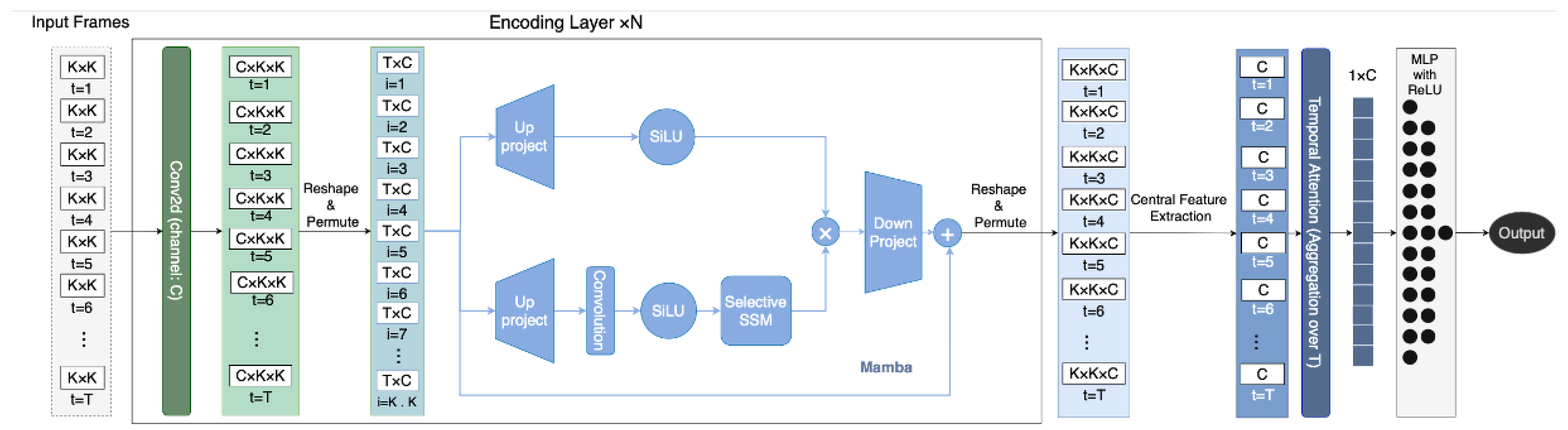
Figure 2.
Spatial distribution of traffic flow intensity across Milan and Trentino regions.
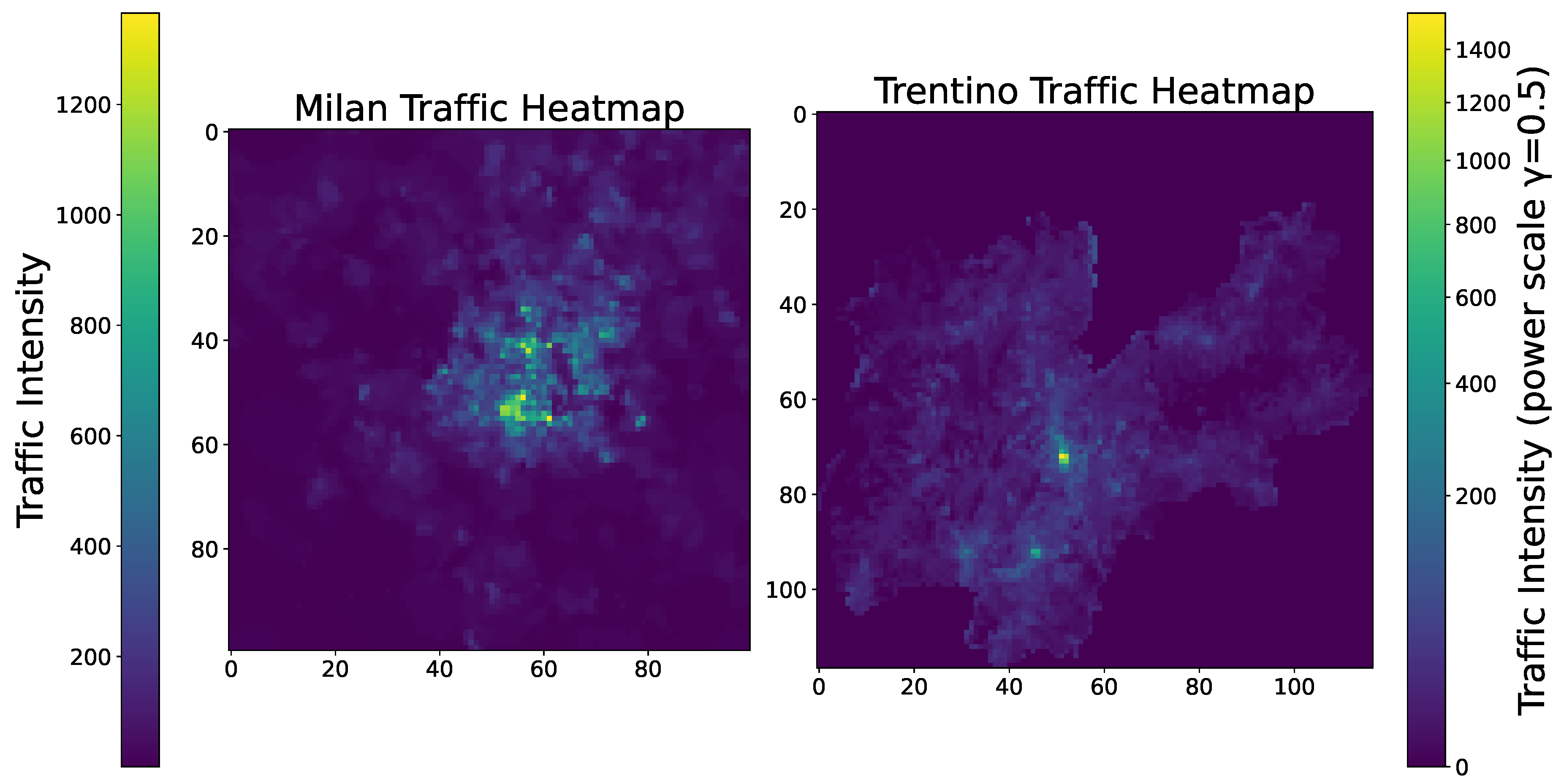
Figure 3.
Lag plot for the autocorrelation of the dataset for the entire grid.
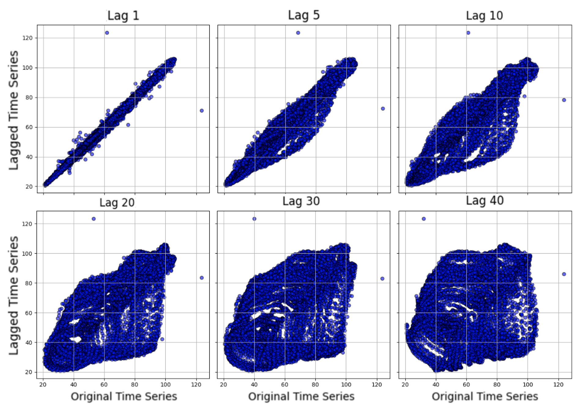
Figure 4.
Traffic volume density distribution across spatial clusters for daytime and nighttime periods (clusters computed on training split only).
Figure 4.
Traffic volume density distribution across spatial clusters for daytime and nighttime periods (clusters computed on training split only).
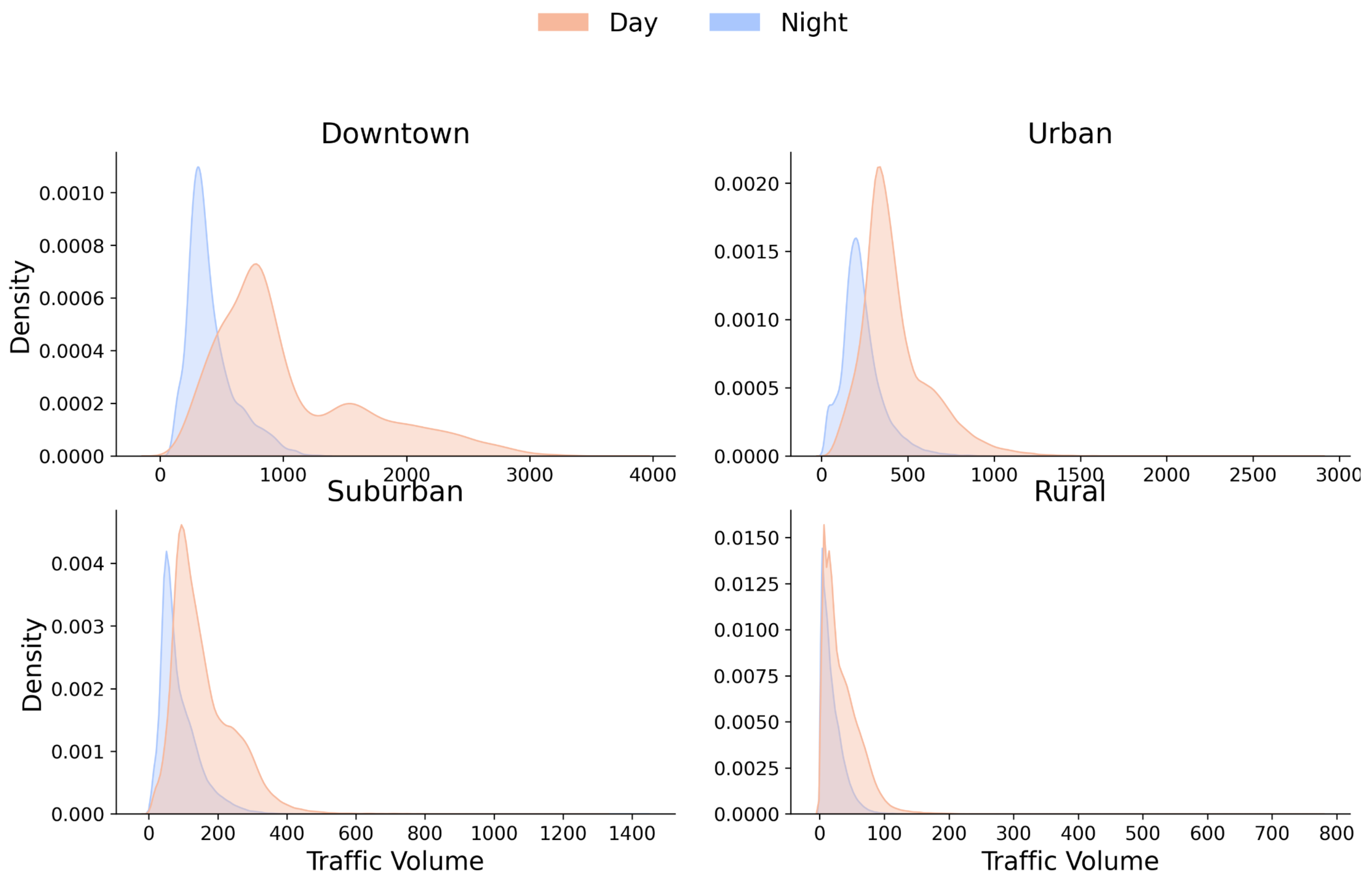
Figure 5.
Traffic volume density distribution across spatial clusters for weekdays and weekends (clusters computed on training split only).
Figure 5.
Traffic volume density distribution across spatial clusters for weekdays and weekends (clusters computed on training split only).
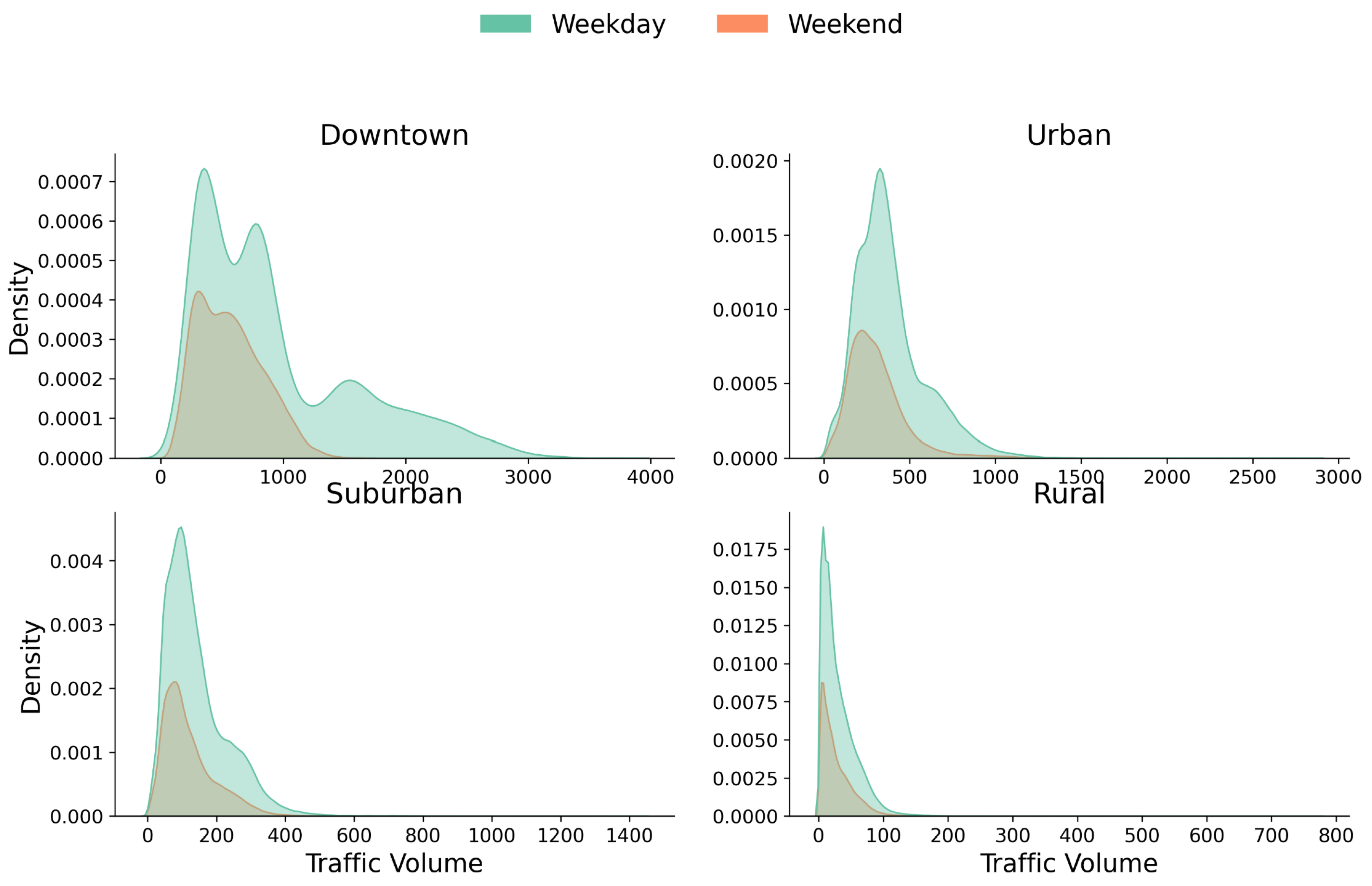
Figure 6.
Selected cells from the Milan’s traffic network. The cells represent different traffic patterns: (a) urban, (b) suburban, (c) rural, and (d) maximum variance cell.
Figure 6.
Selected cells from the Milan’s traffic network. The cells represent different traffic patterns: (a) urban, (b) suburban, (c) rural, and (d) maximum variance cell.
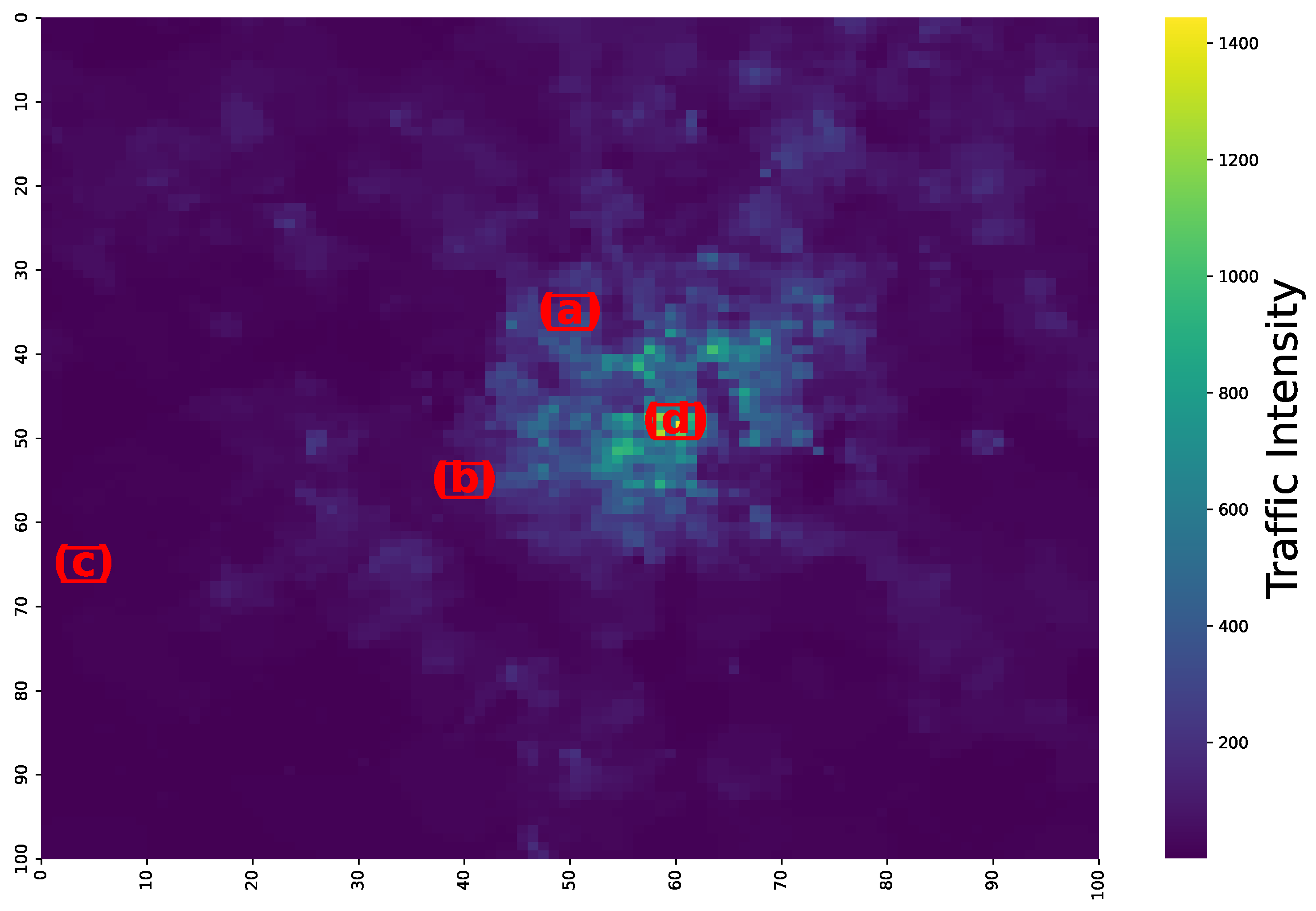
Figure 7.
Week-long traffic predictions from the HiSTM model across four representative cells in Milan’s traffic network. The cells were selected to represent different traffic patterns: (a) urban, (b) suburban, (c) rural, and (d) maximum variance cell. Time is shown in days, with each day containing 144 readings (10-minute intervals)
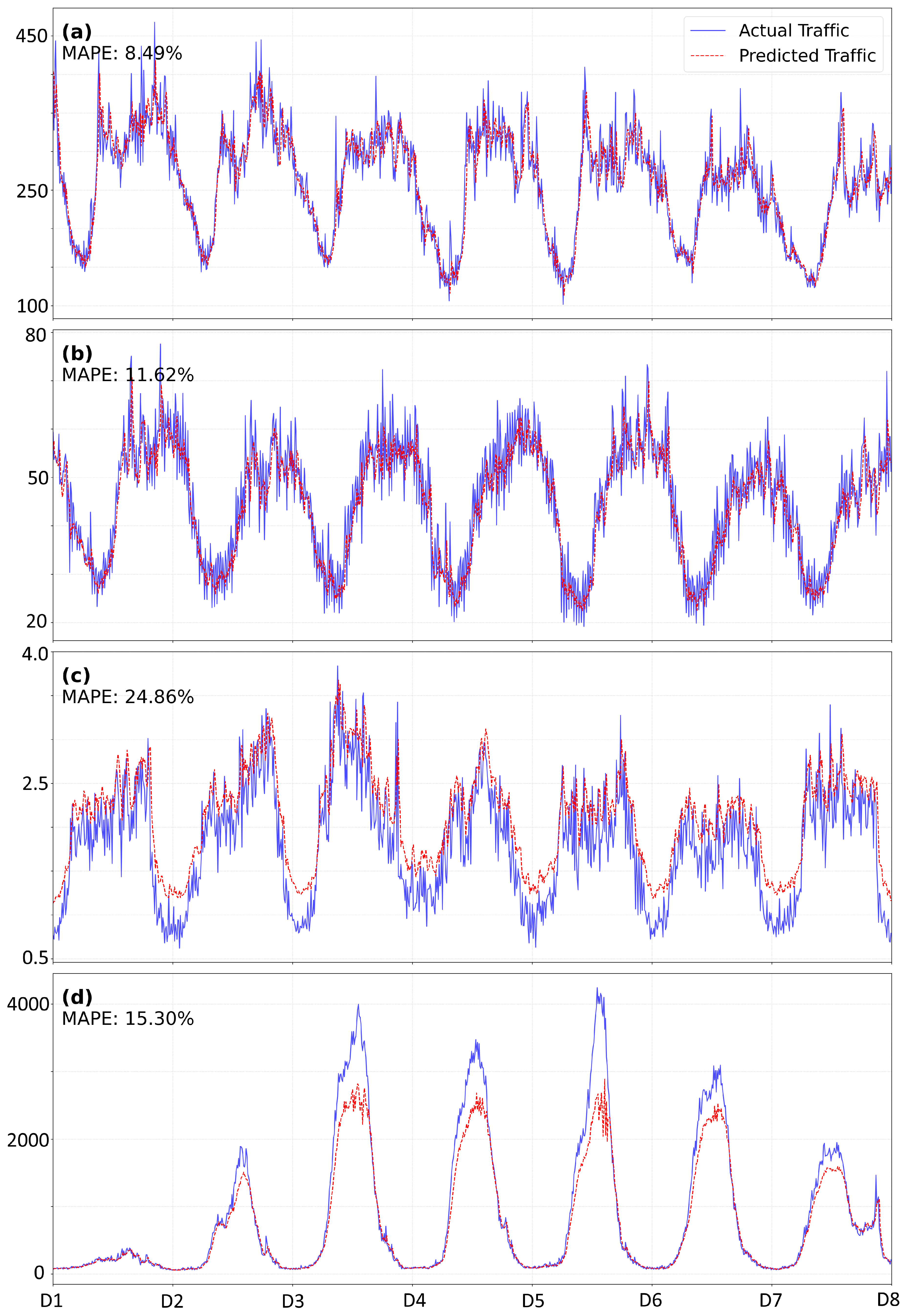
Figure 8.
Spatial distribution of model improvement (Winner Map). Red areas indicate where the global HiSTM achieves lower error than the local LSTM, while blue areas favor the local model
Figure 8.
Spatial distribution of model improvement (Winner Map). Red areas indicate where the global HiSTM achieves lower error than the local LSTM, while blue areas favor the local model
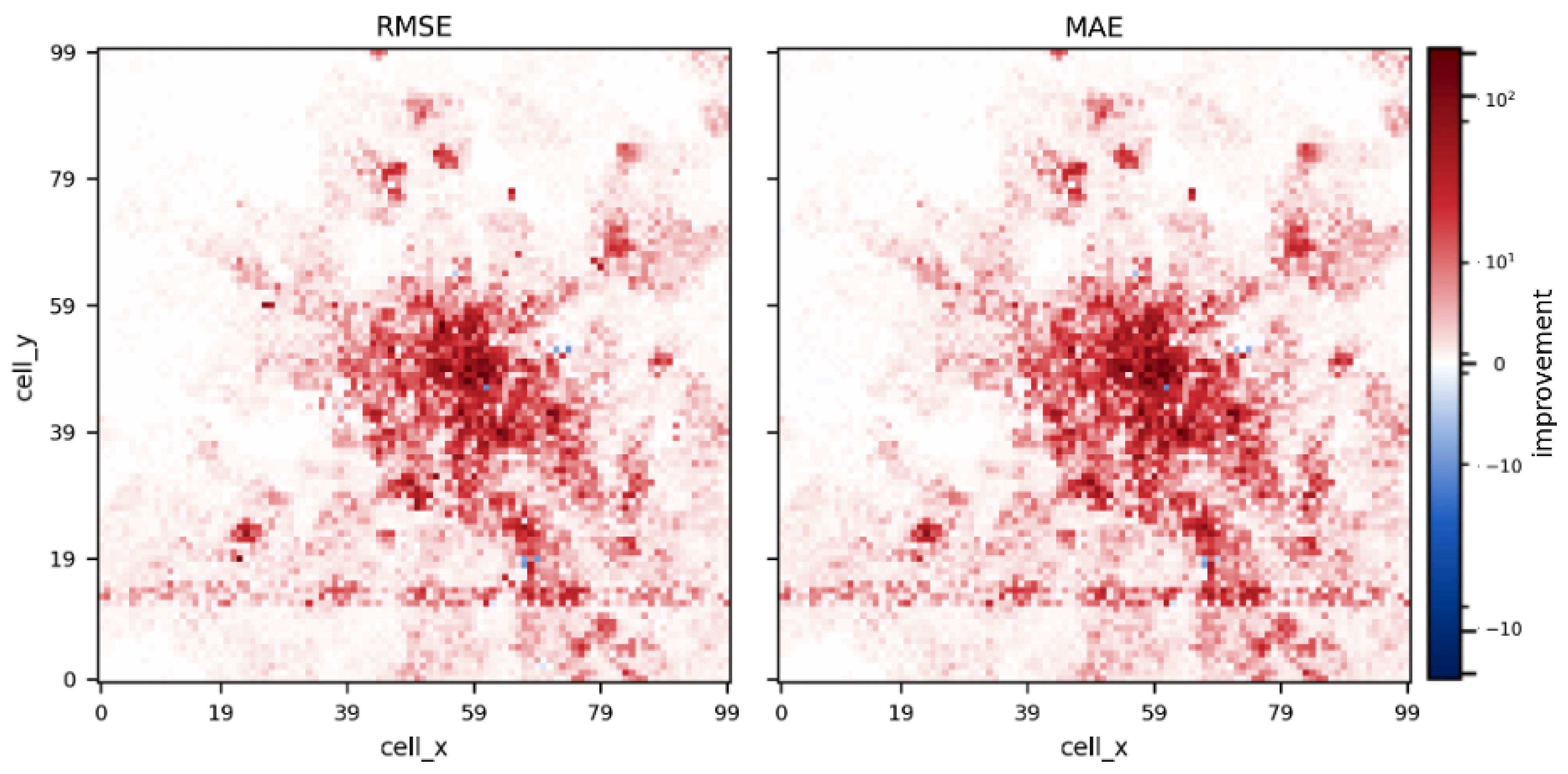
Figure 9.
Cluster-wise RMSE improvement distribution (10k LSTMs vs. HiSTM).
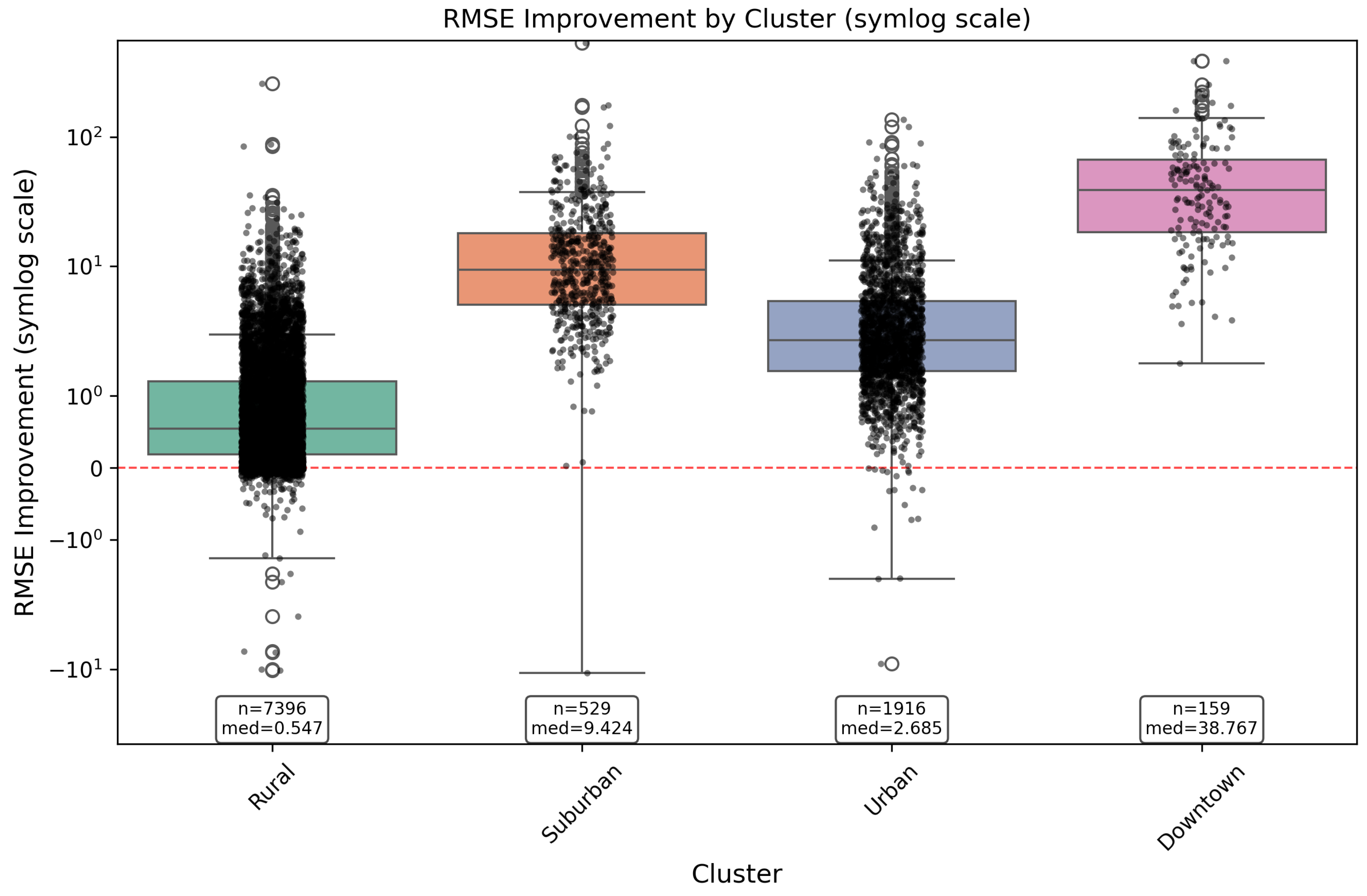
Figure 10.
Distribution of Temporal Attention weights across the lookback window. The near-uniform distribution confirms that HiSTM aggregates global context rather than selecting specific time steps.
Figure 10.
Distribution of Temporal Attention weights across the lookback window. The near-uniform distribution confirms that HiSTM aggregates global context rather than selecting specific time steps.
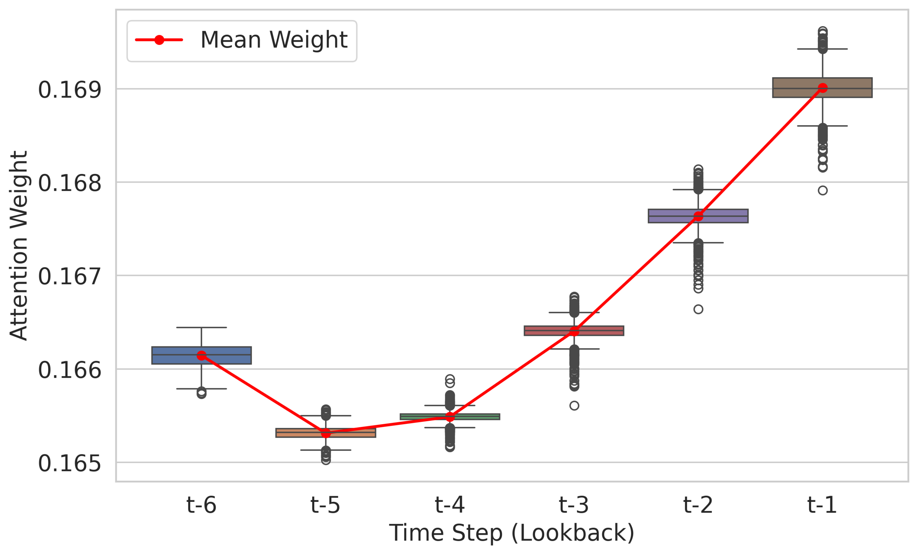
Figure 11.
Case Study 1: Traffic Volume vs. Attention during high variance. The model maintains a stable attention distribution despite traffic fluctuations.
Figure 11.
Case Study 1: Traffic Volume vs. Attention during high variance. The model maintains a stable attention distribution despite traffic fluctuations.
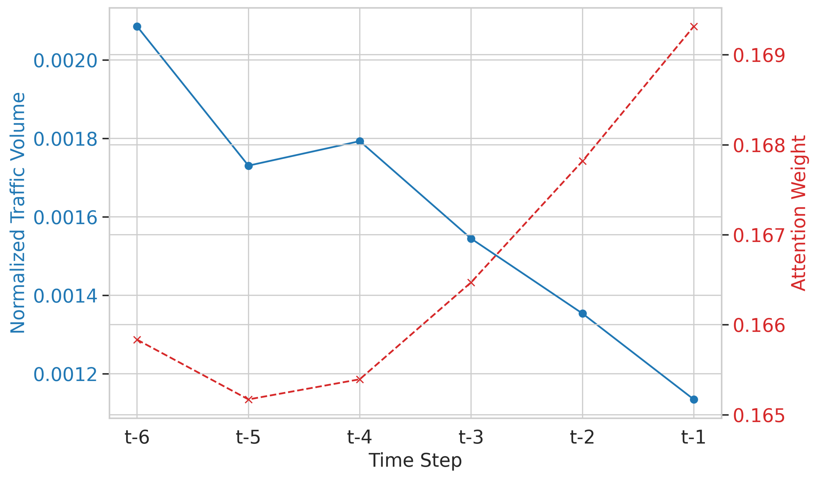
Figure 12.
Case Study 2: Traffic Volume vs. Attention during a ramp-up phase. Despite the increasing traffic trend (green), the attention weights (red) remain distributed, confirming the model aggregates context rather than focusing solely on the most recent step.
Figure 12.
Case Study 2: Traffic Volume vs. Attention during a ramp-up phase. Despite the increasing traffic trend (green), the attention weights (red) remain distributed, confirming the model aggregates context rather than focusing solely on the most recent step.
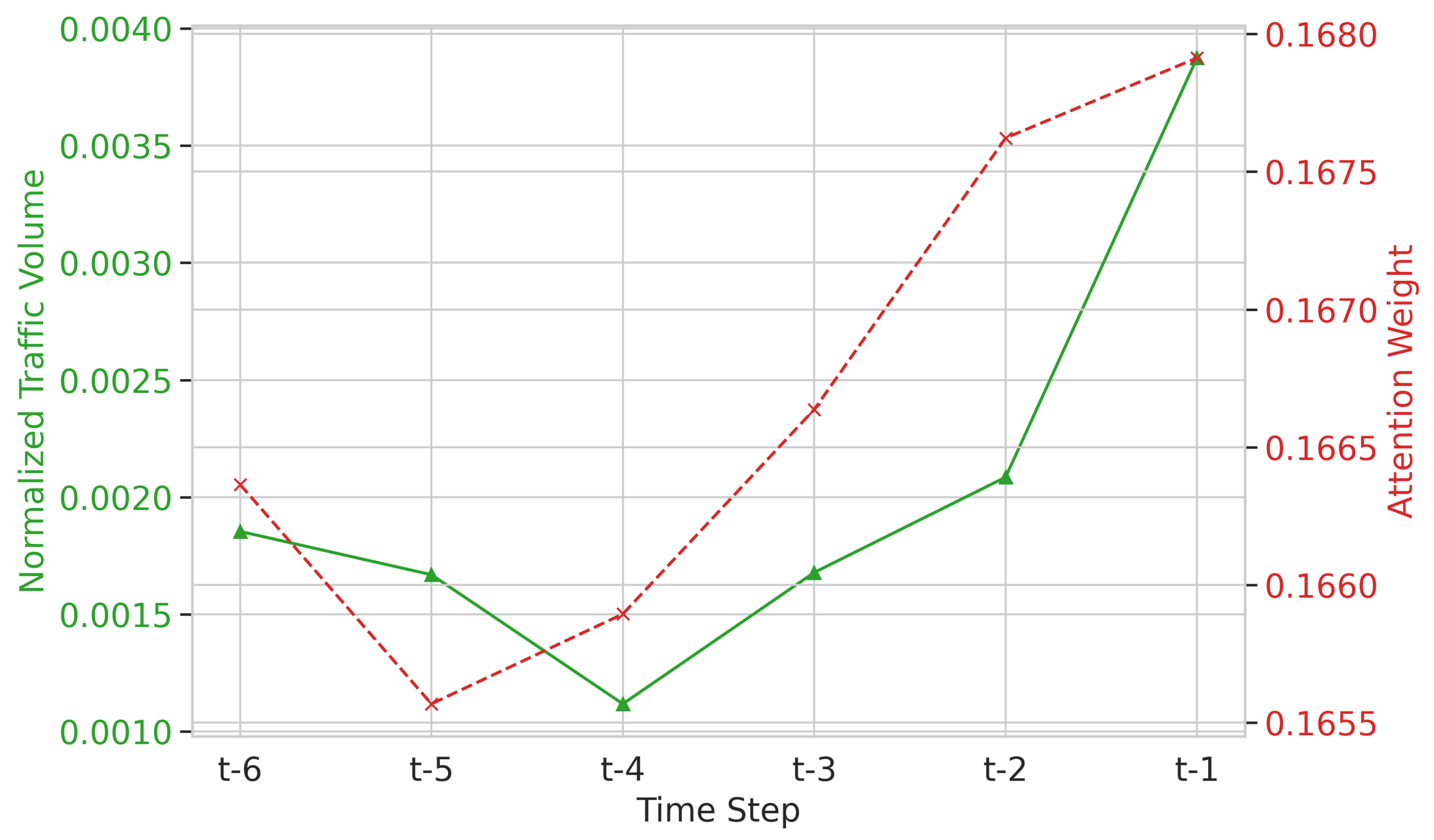
Figure 13.
PCA projection of Mamba’s hidden state trajectory over the 6-step window. The distinct separation of time steps (colors) confirms the SSM maintains a temporal awareness, while the structural consistency across samples indicates robust stable and noise-resistant latent representations.
Figure 13.
PCA projection of Mamba’s hidden state trajectory over the 6-step window. The distinct separation of time steps (colors) confirms the SSM maintains a temporal awareness, while the structural consistency across samples indicates robust stable and noise-resistant latent representations.
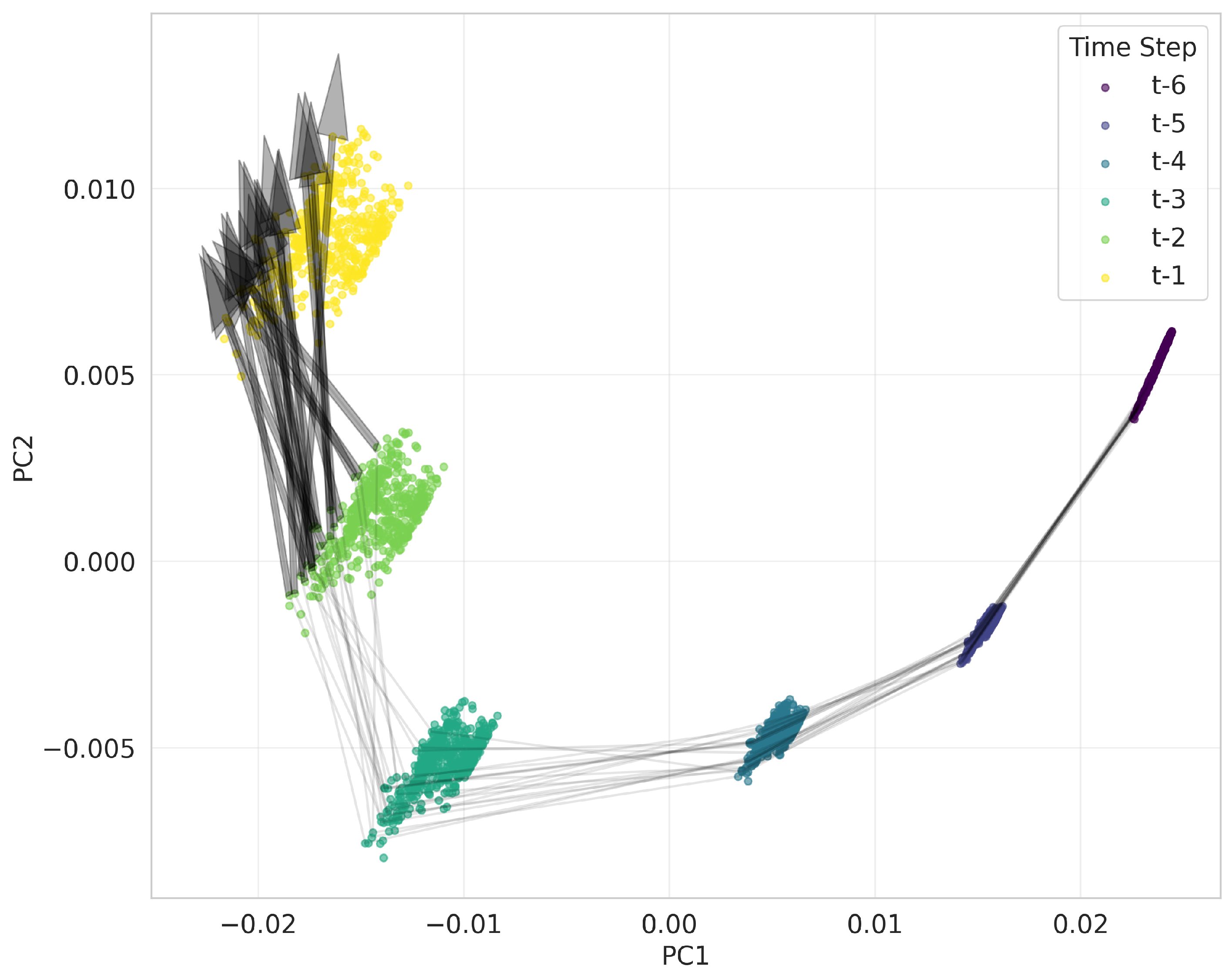
Figure 14.
Sensitivity to Spatial Context by Cluster. The plot shows the percentage increase in MAE when the visible spatial kernel is reduced (from full context at right to at left). Downtown regions are highly dependent on neighbors ( error without them), while Rural regions are largely independent ( error).
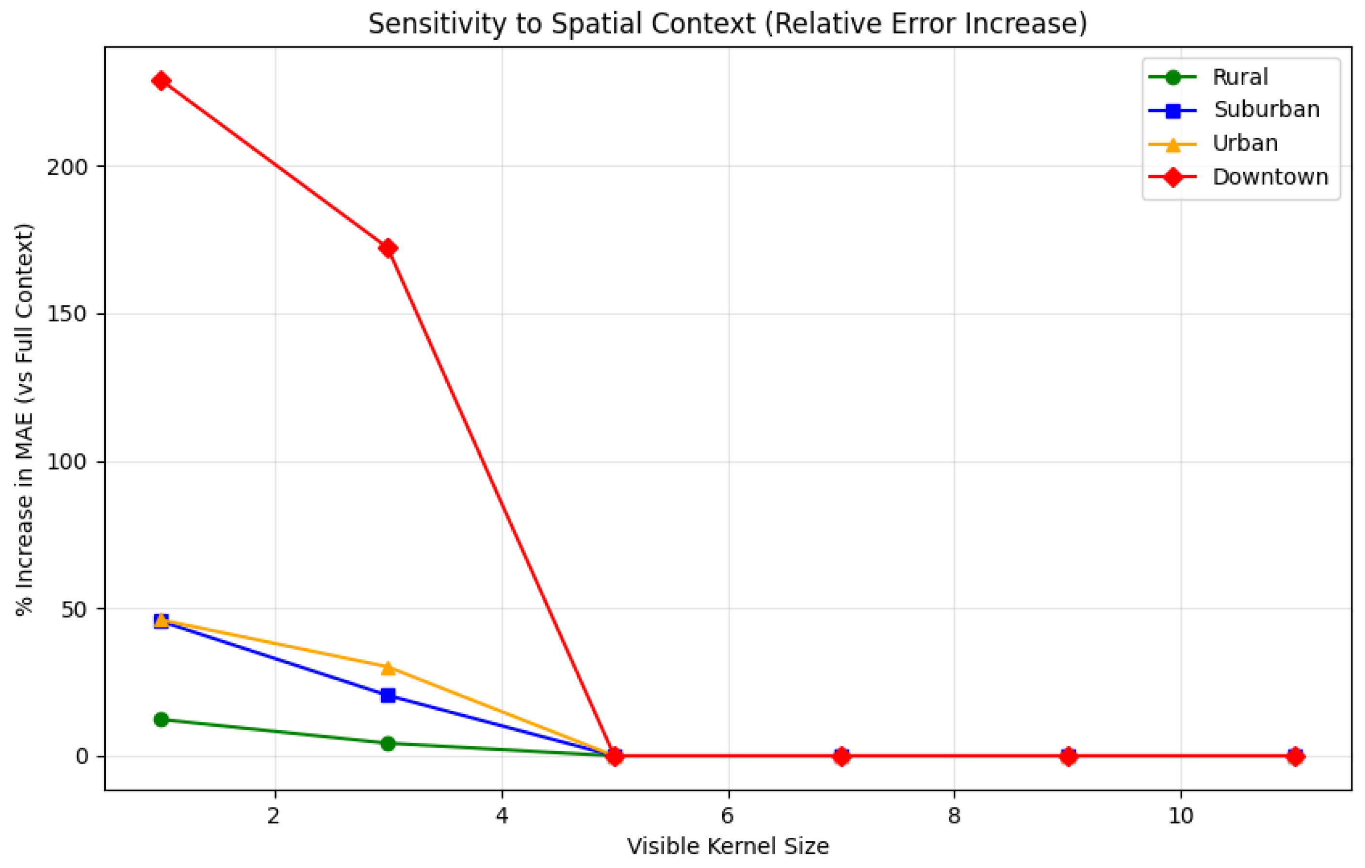

Table 1.
Spatial cluster statistics on Milan, ordered by mean traffic volume (TV); computed on the training split only.
Table 1.
Spatial cluster statistics on Milan, ordered by mean traffic volume (TV); computed on the training split only.
| Cluster | Cells | Mean TV | Std Dev | Min TV | Max TV |
|---|---|---|---|---|---|
| Downtown | 111 | 833.76 | 601.73 | 101.22 | 3,704.96 |
| Urban | 470 | 363.95 | 201.32 | 15.64 | 2,848.75 |
| Suburban | 1655 | 135.62 | 88.06 | 0.64 | 1,434.13 |
| Rural | 7764 | 29.78 | 26.66 | 0.00 | 775.62 |
Table 2.
Single-step Prediction Performance on Milan Dataset. Best model indicated through bold font.
Table 2.
Single-step Prediction Performance on Milan Dataset. Best model indicated through bold font.
| Model | MAE ↓ | RMSE ↓ | R² Score ↑ | SSIM ↑ |
|---|---|---|---|---|
| PatchTST | 20.231 | 45.235 | 0.5635 | 0.9187 |
| STN | 7.3908 | 16.8824 | 0.9546 | 0.9853 |
| VMRNN-B | 7.1659 | 19.0876 | 0.9420 | 0.9843 |
| PredRNN++ | 7.0000 | 19.1650 | 0.9425 | 0.9893 |
| xLSTM | 6.4672 | 15.0901 | 0.9637 | 0.9870 |
| VMRNN-D | 6.4151 | 16.3284 | 0.9575 | 0.9873 |
| STTRE | 5.5558 | 11.4426 | 0.9791 | 0.9917 |
| Autoformer | 5.5850 | 12.2750 | 0.9762 | 0.9920 |
| Informer | 5.4100 | 11.4600 | 0.9792 | 0.9922 |
| TimesNet | 5.3540 | 11.3270 | 0.9797 | 0.9922 |
| HiSTM | 5.2196 | 11.2476 | 0.9799 | 0.9925 |
Table 3.
Performance comparison of models over multiple steps (autoregressive forecasting). Best model indicated through bold font.
Table 3.
Performance comparison of models over multiple steps (autoregressive forecasting). Best model indicated through bold font.
| Step | HiSTM | STN | xLSTM | VMRNN-B | VMRNN-D | |||||
| MAE | RMSE | MAE | RMSE | MAE | RMSE | MAE | RMSE | MAE | RMSE | |
| 1 | 3.87 | 9.54 | 5.28 | 13.05 | 4.64 | 11.86 | 5.11 | 13.75 | 4.62 | 12.25 |
| 2 | 4.38 | 10.95 | 6.44 | 16.29 | 5.62 | 14.63 | 5.08 | 13.85 | 4.61 | 12.36 |
| 3 | 4.85 | 12.06 | 7.39 | 18.54 | 6.47 | 16.78 | 6.06 | 16.33 | 5.35 | 14.30 |
| 4 | 5.56 | 13.42 | 8.59 | 21.05 | 7.50 | 18.95 | 6.83 | 17.64 | 6.08 | 15.49 |
| 5 | 6.09 | 14.62 | 9.55 | 22.94 | 8.34 | 20.58 | 7.45 | 18.91 | 6.59 | 16.54 |
| 6 | 6.69 | 16.02 | 10.59 | 25.01 | 9.23 | 22.38 | 8.24 | 20.38 | 7.30 | 17.87 |
| Step | STTRE | Informer | Autoformer | TimesNet | PatchTST | |||||
| MAE | RMSE | MAE | RMSE | MAE | RMSE | MAE | RMSE | MAE | RMSE | |
| 1 | 4.21 | 9.83 | 7.62 | 19.78 | 8.07 | 21.49 | 7.56 | 19.86 | 29.68 | 73.35 |
| 2 | 4.88 | 11.45 | 8.51 | 23.05 | 9.38 | 24.78 | 8.85 | 24.08 | 30.40 | 73.78 |
| 3 | 5.47 | 12.73 | 9.22 | 25.03 | 10.48 | 26.88 | 10.07 | 26.97 | 31.74 | 74.50 |
| 4 | 6.27 | 14.12 | 9.99 | 27.11 | 11.94 | 30.23 | 11.56 | 30.28 | 33.33 | 75.08 |
| 5 | 6.88 | 15.28 | 10.56 | 28.78 | 13.51 | 34.17 | 12.97 | 33.24 | 34.91 | 76.91 |
| 6 | 7.54 | 16.60 | 11.25 | 31.14 | 15.24 | 38.72 | 14.70 | 37.08 | 36.87 | 79.94 |
Table 4.
Single-step Generalization Performance on Trentino Dataset. Best model indicated through bold font.
Table 4.
Single-step Generalization Performance on Trentino Dataset. Best model indicated through bold font.
| Model | MAE ↓ | RMSE ↓ | R² Score ↑ | SSIM ↑ |
|---|---|---|---|---|
| PredRNN++ | 44.268 | 76.067 | -7.7689 | -0.1305 |
| PatchTST | 5.7460 | 14.398 | 0.6562 | 0.9050 |
| STN | 2.6344 | 7.6370 | 0.9116 | 0.9762 |
| xLSTM | 2.5974 | 8.9235 | 0.8793 | 0.9615 |
| VMRNN-B | 1.9751 | 6.6270 | 0.9334 | 0.9839 |
| STTRE | 1.8132 | 5.0050 | 0.9620 | 0.9903 |
| VMRNN-D | 1.5870 | 5.5754 | 0.9529 | 0.9885 |
| Informer | 1.5310 | 4.9130 | 0.9634 | 0.9915 |
| Autoformer | 1.4960 | 4.9120 | 0.9634 | 0.9915 |
| TimesNet | 1.4070 | 4.7210 | 0.9634 | 0.9915 |
| HiSTM | 1.3870 | 4.8134 | 0.9649 | 0.9916 |
Table 5.
Missing Data in Training and Testing Data by Last Observation Carried Forward.
| Train % | Model | Test 0% | Test 10% | Test 20% | Test 30% | ||||
|---|---|---|---|---|---|---|---|---|---|
| MAE | RMSE | MAE | RMSE | MAE | RMSE | MAE | RMSE | ||
| STN | 5.3926 | 11.9684 | 5.3926 | 11.9681 | 5.3924 | 11.9682 | 5.3919 | 11.9648 | |
| VMRNN-D | 5.8185 | 13.0920 | 5.8184 | 13.0919 | 5.8185 | 13.0920 | 5.8183 | 13.0875 | |
| STTRE | 5.5143 | 11.6435 | 5.5199 | 11.7132 | 5.5139 | 11.6600 | 5.5089 | 11.6345 | |
| 0% | TimesNet | 5.3127 | 11.6955 | 5.3124 | 11.6950 | 5.3124 | 11.6948 | 5.3114 | 11.6906 |
| Informer | 5.2306 | 11.2889 | 5.2304 | 11.2885 | 5.2304 | 11.2883 | 5.2298 | 11.2864 | |
| Autoformer | 5.2959 | 11.5546 | 5.2956 | 11.5541 | 5.2957 | 11.5540 | 5.2946 | 11.5505 | |
| HiSTM | 5.1462 | 10.9949 | 5.1461 | 10.9945 | 5.1460 | 10.9944 | 5.1451 | 10.9915 | |
| STN | 5.3215 | 11.5511 | 5.3213 | 11.5505 | 5.3212 | 11.5505 | 5.3205 | 11.5443 | |
| VMRNN-D | 5.8472 | 13.3272 | 5.8471 | 13.3272 | 5.8472 | 13.3272 | 5.8470 | 13.3228 | |
| STTRE | 5.5204 | 11.6472 | 5.5086 | 11.5750 | 5.5094 | 11.6136 | 5.5136 | 11.6360 | |
| 10% | TimesNet | 5.6641 | 11.5155 | 5.6637 | 11.5147 | 5.6639 | 11.5148 | 5.6628 | 11.5118 |
| Informer | 5.2386 | 11.2464 | 5.2384 | 11.2460 | 5.2383 | 11.2457 | 5.2378 | 11.2441 | |
| Autoformer | 5.5687 | 11.6021 | 5.5684 | 11.6013 | 5.5684 | 11.6014 | 5.5679 | 11.5998 | |
| HiSTM | 5.1762 | 11.0894 | 5.1765 | 11.0972 | 5.1765 | 11.0972 | 5.1754 | 11.0934 | |
Table 6.
Comparison of MAE Performance on RU Dataset
| Model | ThPut-S | PRB-A | PRB-S | BLER-C | BLER-A |
|---|---|---|---|---|---|
| Autoformer | 72.6006 | 333.5814 | 335.3883 | 33.6488 | 0.0039 |
| TimesNet | 70.8017 | 335.0931 | 337.2877 | 34.8186 | 0.0038 |
| Informer | 70.3382 | 379.5331 | 342.9107 | 33.7061 | 0.0037 |
| xLSTM | 71.8190 | 379.0264 | 341.4050 | 39.4904 | 0.0038 |
| STN | 71.0536 | 334.5146 | 339.6057 | 33.2997 | 0.0041 |
| STTRE | 72.1947 | 348.5375 | 353.1801 | 33.8897 | 0.0038 |
| HiSTM | 70.0721 | 328.2811 | 324.2433 | 32.2687 | 0.0037 |
Table 7.
Cluster-wise Evaluation of HiSTM: Cluster-Specific (CS), Global-Blind (GB), ClusterFiLM (CF), ClusterFiLM-Unbalanced (CF-U), and Global-Aware (GA) Models. Bold values indicate the best (lowest) performance per metric.
Table 7.
Cluster-wise Evaluation of HiSTM: Cluster-Specific (CS), Global-Blind (GB), ClusterFiLM (CF), ClusterFiLM-Unbalanced (CF-U), and Global-Aware (GA) Models. Bold values indicate the best (lowest) performance per metric.
| Cluster | Metric | CS | GB | CF | CF-U | GA |
|---|---|---|---|---|---|---|
| MAE | 42.61 | 32.45 | 35.44 | 33.64 | 32.57 | |
| Downtown | RMSE | 60.20 | 45.88 | 49.50 | 47.23 | 46.40 |
| MASE | 0.119 | 0.091 | 0.099 | 0.094 | 0.091 | |
| MAE | 22.34 | 21.54 | 22.12 | 21.91 | 21.24 | |
| Urban | RMSE | 30.86 | 29.83 | 30.46 | 30.14 | 29.73 |
| MASE | 0.143 | 0.138 | 0.141 | 0.140 | 0.136 | |
| MAE | 9.00 | 8.95 | 9.10 | 9.16 | 8.91 | |
| Suburban | RMSE | 13.27 | 13.24 | 13.37 | 13.33 | 13.24 |
| MASE | 0.132 | 0.132 | 0.134 | 0.135 | 0.131 | |
| MAE | 2.49 | 2.50 | 2.63 | 2.55 | 2.52 | |
| Rural | RMSE | 4.28 | 4.29 | 4.38 | 4.39 | 4.32 |
| MASE | 0.131 | 0.132 | 0.139 | 0.135 | 0.133 | |
| MAE | 5.31 | 5.15 | 5.33 | 5.26 | 5.13 | |
| Aggregate | RMSE | 11.96 | 10.99 | 11.33 | 11.16 | 11.02 |
| MASE | 0.132 | 0.128 | 0.093 | 0.091 | 0.089 |
Table 8.
HiSTM Performance Across Varying Kernel Sizes
| Metric | 3x3 | 5x5 | 7x7 | 9x9 | 11x11 | 13x13 |
|---|---|---|---|---|---|---|
| MAE | 5.1919 | 5.1572 | 5.1874 | 5.1303 | 5.1462 | 5.1425 |
| RMSE | 11.1146 | 11.1425 | 11.0731 | 11.0600 | 10.9949 | 10.9666 |
Table 9.
HiSTM Performance with Window Variations (LD: last-day kernel, LW: last-week kernel)
| Look-back Window |
Window Only | +LD | +LD+LW | |||
|---|---|---|---|---|---|---|
| MAE | RMSE | MAE | RMSE | MAE | RMSE | |
| 1 (10min) | 5.7593 | 12.1600 | 5.5517 | 11.6985 | 5.3793 | 11.2973 |
| 3 (30min) | 5.2299 | 11.2418 | 5.1163 | 10.9998 | 5.0850 | 10.8066 |
| 6 (1hr) | 5.1572 | 11.1425 | 5.0663 | 10.9067 | 4.9109 | 10.3662 |
| 9 (1.5hr) | 5.1269 | 11.0545 | 5.0080 | 10.6847 | 4.8633 | 10.2967 |
| 12 (2hr) | 5.1426 | 11.0745 | 5.0312 | 10.6732 | 4.9204 | 10.4330 |
| 24 (4hr) | 5.1342 | 10.9946 | 5.0293 | 10.7380 | 4.9054 | 10.4225 |
| 36 (6hr) | 5.1146 | 11.0137 | 5.0461 | 10.7686 | 4.9309 | 10.4487 |
Table 10.
Model Comparison
| Model | Parameter Count |
Size (MB) |
GPU (MB) |
Inference (ms) |
MACs |
|---|---|---|---|---|---|
| PredRNNpp | 2,223,873 | 8.48 | 23.52 | 6.38 | |
| VMRNN-D | 1,506,498 | 5.75 | 15.47 | 18.58 | |
| xLSTM | 607,753 | 2.32 | 13.69 | 1.01 | |
| PatchTST | 593,665 | 4.71 | 30.98 | 0.46 | |
| STN | 576,755 | 2.20 | 11.34 | 2.46 | |
| Autoformer | 442,241 | 4.13 | 13.28 | 2.06 | |
| TimesNet | 295,425 | 1.13 | 11.95 | 2.11 | |
| Informer | 245,249 | 3.38 | 12.52 | 1.37 | |
| STTRE | 165,380 | 0.63 | 58.07 | 4.54 | |
| VMRNN-B | 137,282 | 0.52 | 9.77 | 8.16 | |
| HiSTM | 33,794 | 0.13 | 10.63 | 1.19 |
Disclaimer/Publisher’s Note: The statements, opinions and data contained in all publications are solely those of the individual author(s) and contributor(s) and not of MDPI and/or the editor(s). MDPI and/or the editor(s) disclaim responsibility for any injury to people or property resulting from any ideas, methods, instructions or products referred to in the content. |
© 2026 by the authors. Licensee MDPI, Basel, Switzerland. This article is an open access article distributed under the terms and conditions of the Creative Commons Attribution (CC BY) license (http://creativecommons.org/licenses/by/4.0/).
Copyright: This open access article is published under a Creative Commons CC BY 4.0 license, which permit the free download, distribution, and reuse, provided that the author and preprint are cited in any reuse.


