
Submitted:
17 January 2026
Posted:
19 January 2026
You are already at the latest version
Abstract
Time series forecasting represents one of the most critical challenges in contemporary data science and machine learning, with applications spanning finance, energy systems, weather prediction, traffic management, supply chain optimization, and healthcare. This comprehensive review examines and compares three prominent forecasting methodologies: Autoregressive Integrated Moving Average (ARIMA), Long Short-Term Memory (LSTM) neural networks, and Prophet. These models embody distinct paradigms—traditional statistical methods, deep learning architectures, and automated trend-based analysis respectively. Through systematic synthesis of recent literature and empirical studies from 2018–2025, this review analyzes theoretical foundations, practical implementations, strengths, limitations, and optimal application contexts. Our findings reveal that ARIMA exhibits superior performance for simple linear patterns (MAPE 3.2–13.6%), LSTM demonstrates exceptional capability in capturing complex non-linear dependencies with 84–87% error reduction vs. ARIMA, while Prophet excels in handling business time series with strong seasonality (MAPE 2.2–24.2%). Model selection depends critically on data characteristics, forecasting horizon, computational resources, and application requirements. This review synthesizes over two decades of empirical findings to provide principled guidance for practitioners in model selection and implementation.
Keywords:
time series forecasting
; ARIMA
; LSTM
; prophet
; comparative analysis
1. Introduction
Time series forecasting represents one of the most fundamental and pervasive challenges in data science and machine learning, with applications spanning virtually all domains [1,2,3]. From financial markets predicting stock prices and currency movements [4], to environmental systems tracking climate patterns [5], to industrial applications forecasting energy consumption and manufacturing outputs [6], to healthcare systems predicting patient demand and disease spread [7,8]—accurate forecasting enables informed decision-making [1,9]. Over the past seven decades, numerous forecasting methodologies have been developed, each with distinct theoretical foundations, computational requirements, and practical applications [12,13,14].
This capability enables organizations to optimize capacity planning, set realistic targets, detect anomalies, manage risks, and allocate resources effectively [2,3]. The core mission of time series analysis is both deceptively simple and profoundly challenging: to extract meaningful statistical patterns from historical observations to predict future values with acceptable accuracy [10,11].
The history of time series forecasting spans over a century, beginning with econometric work by Jan Tinbergen (1939) [12]. The field has undergone dramatic evolution through distinct paradigms.
Classical statistical methods emerged in the 1950s–1980s with ARIMA and exponential smoothing pioneered by Box and Jenkins (1970) [15,16,17]. Nonlinear models emerged in the 1980s–1990s with TAR models and ARCH/GARCH for volatility clustering [19,20]. Machine learning approaches dominated the 1990s–2000s with neural networks, SVM, and Gaussian process regression [21,22]. Deep learning emerged in the 2010s–present era with LSTM [23,24], CNN, GRU [25], Transformer models, and attention mechanisms [26,27,28].
In the current era, three modeling paradigms dominate contemporary forecasting practice: ARIMA—Classical statistical approach grounded in stochastic process theory [15,29], LSTM—Deep learning paradigm capturing nonlinear temporal patterns [23,24,30], and Prophet—Pragmatic hybrid designed specifically for business-scale forecasting [31,32,33].
This comprehensive review addresses a critical knowledge gap regarding when each model is most appropriate and how practitioners should select optimal forecasting approaches for specific applications [1,2,34]. Recent empirical studies comparing these models demonstrate varied results depending on dataset characteristics, forecasting horizons, and data complexity [2,34,35]. This review aims to: provide comprehensive technical overview of ARIMA, LSTM, and Prophet methodologies and systematically compare theoretical foundations and practical implementations.
2. Theoretical Framework
2.1. ARIMA: Autoregressive Integrated Moving Average
ARIMA(p, d, q) combines three primary components . Autoregression (AR, order p) captures linear relationships with lagged observations:
Integration (I, order d) applies differencing to transform non-stationary time series into stationary series:
Moving Average (MA, order q) models the relationship between observations and residual errors:
For seasonal data, Seasonal ARIMA (SARIMA) extends the framework: SARIMA(p, d, q)(P, D, Q)_S [15,29,48,49,50].
Figure 1 shows ARIMA methodology flowchart showing iterative steps from stationarity testing through ACF/PACF analysis, parameter estimation, and residual diagnostics. Feedback loops ensure model adequacy before forecast generation, emphasizing the systematic nature of ARIMA model development.
ARIMA models offer several significant advantages: mathematically interpretable with clear parameter meanings [15,29], computationally efficient requiring minimal resources (0.5–5 seconds training) [35,36,51], well-established theoretical foundation with decades of successful applications [15,16,29], excellent performance for simple linear patterns and stationary data [15,29,51], and requires minimal data (200+ observations) [15,29,35]. However, ARIMA models present notable limitations: requires stationarity or differencing [15,29,44], poor at capturing non-linear relationships [1,2,35], struggles with high-frequency volatile data [35,36,51], requires manual parameter tuning [15,29], assumes constant statistical properties [1,35], and limited adaptability to changing data characteristics [35,51].
2.2. LSTM: Long Short-Term Memory Networks
LSTM networks are specialized RNNs designed to address the vanishing gradient problem [23,24,30,54]. The LSTM architecture comprises memory cells with three primary gating mechanisms. The forget gate controls information retention:
The input gate determines which new information updates the cell state:
The output gate selects which information flows to the next layer:
LSTM effectively mitigates the vanishing gradient problem through constant error carousels (CEC) and multiplicative interactions [23,24,54], enabling the network to learn long-term dependencies spanning hundreds of time steps [23,30].
Figure 2 shows LSTM neural network architecture showing input sequences flowing through stacked LSTM layers containing forget, input, and output gates. The gating mechanisms enable capture of long-term dependencies and complex non-linear patterns. The Dense output layer produces one-step-ahead forecasts.
LSTM networks demonstrate several important advantages: excellent capability capturing long-term dependencies and non-linear patterns [23,24,30,55], superior performance on complex, highly volatile data (84–87% error reduction vs. ARIMA) [1,35,51,56], effective with non-stationary time series without explicit preprocessing [1,35,56], can simultaneously process multiple input features (multivariate forecasting) [1,23,30,56], flexible architecture supporting custom designs [30,57], and learns complex temporal patterns automatically [23,30].
However, LSTM models present substantial challenges: requires substantially more training data (typically 5,000+ observations) [1,35,51,56], high computational requirements during training (5 minutes to 2+ hours) [1,35,51], “black box” nature complicates interpretability [1,2,35,56], extremely sensitive to hyperparameter choices and initialization [1,35,56,57], prone to overfitting on smaller datasets [1,35,56,57], performance can exhibit high variance [1,35,56], requires careful data normalization [35,56,57], and substantial GPU resources needed [1,35,51].
2.3. Prophet: Automated Forecasting Procedure
Prophet employs an additive decomposable time series model combining multiple interpretable components [31,32,33]:
where g(t) represents the trend component (piecewise linear or logistic growth), s(t) models seasonal patterns using Fourier series:
h(t) captures holiday effects modeled as external regressors:
and ε_t represents error or noise.
Figure 3 shows Prophet decomposes time series into four interpretable components: trend g(t), seasonality s(t), holiday effects h(t), and error term ε_t and this demonstrates how Prophet makes individual components explicit for business interpretation.
Prophet models offer distinct advantages: designed specifically for business time series forecasting [31,32,33], automatic handling of missing data and outliers [31,32,33,58,59], requires minimal hyperparameter tuning [31,32,33,58], highly interpretable components [31,32,33], robust to structural changes [31,32,33], handles irregular seasonality and holiday effects [58,59], uses Bayesian inference providing uncertainty quantification [31,32,33], and fast training (30 seconds to 5 minutes) [35,36,59].
However, Prophet models have notable limitations: less effective with short-term fluctuations and high-frequency data [1,31,32,35], assumes additive model structure with limited multiplicative seasonality handling [31,32,33], performance challenges with highly volatile data lacking seasonality [1,31,32], limited capacity for capturing complex non-linear relationships [1,2,31], may oversmooth data [58,59], primarily designed for univariate forecasting [31,32,33], and performance degrades on non-seasonal data [1,31,32].
3. Literature Review
3.1. Performance Metrics and Empirical Studies
3.2. Domain-Specific Applications
- Financial Forecasting: Comparative studies on financial datasets demonstrate significant performance variations [4,35,51,56]. LSTM achieved 84–87% reduction in error rates compared to ARIMA [1,35,51,56], with MAPE values of 4.06–26.02% for hourly predictions versus ARIMA’s 7.21–43.48% [35,51,56]. ARIMA maintained consistent performance (MAPE 3.20–13.60%) for daily and longer forecasts [35,51]. Stock price prediction studies show LSTM achieved R² = 0.96–0.97 on test datasets [51,56], while hybrid models achieved R² = 0.98–0.99 on complex stock data [39,62].
- Energy and Environmental Applications: Renewable energy forecasting reveals LSTM demonstrated R² = 0.986 on wind power prediction [37], while hybrid GRU-attention models achieved 75% error reduction over traditional methods [63]. Prophet proved effective for solar power with clear daily patterns (MAPE < 10%) [5,32,37], and SARIMA remained comparable to LSTM on seasonal energy data (MAPE 6–8%) [48,50]. CNN-LSTM combinations improved accuracy by 20–30% on multi-step forecasting [37,64]. Air quality forecasting shows LSTM outperformed ARIMA by 15–25% on PM2.5 prediction [5,65], with ensemble methods combining ARIMA, LSTM, and Prophet achieving best performance [66].
- Healthcare and Disease Prediction: COVID-19 case forecasting demonstrates hybrid ARIMA-LSTM achieved lowest errors (MSE = 2,501,541; MAPE = 6.43%) [8,41], while LSTM outperformed ARIMA by 30–40% on pandemic data [7,8,41]. Prophet handled holiday effects well but struggled with volatile spikes [7,8], and ensemble models combining all three approaches improved predictions 15–20% [7,42].
- Traffic and Retail Applications: Traffic prediction studies show LSTM outperformed ARIMA for short-term traffic prediction [6,34,68], while ARIMA maintained competitive performance for daily aggregates (MAPE 2.9%) [34,51]. Hybrid LSTM-GRU models achieved 85–92% accuracy on hourly traffic [68]. For sales forecasting, daily forecasting shows ARIMA (MAPE 2.9–13.6%), Prophet (MAPE 2.2–24.2%), and LSTM (MAPE 6.6–20.8%) [35,51], while Prophet excels for retail with strong weekly/yearly seasonality [2,31,32,35].
3.3. Forecasting Horizon and Data Characteristics
Different forecasting horizons substantially influence model performance [1,2,34,35,51]. For short-term forecasting (hours to 1 day), LSTM generally provides superior performance with lower error metrics [1,35,51], though ARIMA maintains competitive performance for 1–2 day horizons [35,51], while Prophet struggles with hourly predictions [35,51,59]. Medium-term forecasting (days to weeks) shows ARIMA and LSTM with comparable performance [1,34,35], though ARIMA’s advantage increases as horizon extends [1,35,51], and Prophet shows improved performance with clearer seasonal patterns [2,32,35]. Long-term forecasting (weeks to months) demonstrates ARIMA’s superior performance capturing trends [1,35,51], while LSTM performance degrades without additional external features [1,35,51], yet Prophet excels with strong seasonal components (MAPE < 10%) [2,31,32]. The strengths of the models shown in Table 2.
3.4. Research Gap and Problem Statement
The common gap across the literature is that they mostly optimize accuracy on local, proprietary datasets but do not address generalization, uncertainty, interpretability, or deployment needs in a systematic way. Models are typically trained and evaluated on single-site or single-market data (e.g., Dhaka renewables, one UK PV farm, one Saudi real estate stock), using short or narrow time spans and non-standard datasets, which prevents fair comparison between studies and limits confidence that results will hold in other regions or under future conditions. Deep learning models such as LSTM, CNN-LSTM, and GRU often outperform classical approaches in reported metrics, but they are treated as black boxes without SHAP/LIME analysis, feature importance, or attention visualization, so decision-makers cannot see which inputs drive forecasts or how models behave under regime shifts like climate change, policy changes, or market shocks. Evaluation is almost always based on a single temporal split with generic error measures (MAE, RMSE, MAPE, R²), with no walk-forward cross-validation, no prediction intervals or probabilistic scores, and no statistical tests (e.g., Diebold–Mariano) to check if differences between models are significant, which means small apparent gains may be due to randomness rather than real superiority. Finally, most works remain offline experiments: they neither quantify computational cost nor test real-time behavior, drift detection, or robustness in resource-constrained settings, so it remains unclear whether the proposed models can actually be deployed and maintained in the critical infrastructures (energy, traffic, water, finance) they aim to support. The primary objective of this comparative study is to systematically evaluate and contrast the performance, applicability, and limitations of three distinct classes of time series forecasting models: ARIMA (statistical/classical), LSTM (deep learning), and Prophet (hybrid/additive). By analyzing these models across diverse domains—including finance, energy, healthcare, environmental monitoring, and manufacturing—this survey aims to:
1) Quantify performance differences using standard metrics (RMSE, MAE, MAPE) to determine which model excels in handling linear vs. nonlinear patterns, short-term vs. long-term horizons, and stationary vs. non-stationary data.
2) Compare models based on computational efficiency, training time, data requirements (e.g., minimum history needed), and ease of implementation.
3) Examine how each model handles real-world data challenges such as missing values, outliers, seasonality, and structural breaks (e.g., market crashes, pandemics).
4) Establish clear guidelines for practitioners to select the most appropriate model based on specific domain constraints (e.g., interpretability needs in healthcare vs. high-frequency precision in finance).
3.5. Hybrid and Ensemble Approaches
ARIMA-LSTM Hybrid Models. The rationale involves decomposing forecasting into linear and non-linear components [39,40,41]. ARIMA captures linear trends and seasonal components, while LSTM captures non-linear residuals and complex patterns, with final forecast: ŷ_t = ŷ_t^ARIMA + ŷ_residuals,t^LSTM [39,40]. Empirical performance shows outperformance of single models by 5–20% [39,40,41]. COVID-19 hybrid model achieved MSE = 2,501,541 versus ARIMA (2,568,836) and LSTM (3,352,686) [8,41], while stock price hybrid achieved R² = 0.98–0.99 versus ARIMA (0.85–0.90) and LSTM (0.92–0.95) [39,62].
Ensemble Methods. Weighted ensemble combinations employ simple averaging with equal weights, weighted averaging optimizing weights via cross-validation (50% ARIMA, 30% LSTM, 20% Prophet typical), and dynamic weighting adjusting based on recent accuracy. Performance improvements achieve 5–20% error reduction compared to best individual model, reducing variance across time periods, proving more robust to concept drift and structural breaks and providing uncertainty bands for risk assessment. The Table 3 shows the hybrid and ensemble performance of the models.
3.6. Methodology and Research Design
This research adopts a comprehensive comparative experimental design to evaluate three distinct time-series forecasting paradigms: ARIMA (classical statistical), LSTM (deep learning), and Prophet (modern business-oriented). The research follows a structured four-stage methodology. In the first stage, data selection and preparation, one or more real-world univariate time-series relevant to diverse application domains are selected, including sales, energy demand, oil production, and water consumption. Each series is split into training and testing segments using strict temporal ordering—no random shuffling—with a typical 70–80% training and 20–30% testing split. Additional validation splits, such as rolling or walk-forward validation, are generated where needed to ensure robust model selection and prevent data leakage. In the second stage, model development proceeds through three parallel independent pipelines. ARIMA is implemented as the classical statistical baseline, LSTM as the deep learning baseline, and Prophet as the modern business-oriented baseline. Each model is trained independently on identical training data and subsequently evaluated on identical test data to ensure fair comparison. The third stage involves comprehensive model evaluation and comparison using standard error metrics (MAE, RMSE, MAPE) and, where applicable, coefficient of determination (R²) to quantify predictive performance. Computational aspects are measured including training time, inference time, and resource requirements distinguishing between CPU-only and GPU-required implementations. Models are compared across multiple dimensions: accuracy, computational efficiency, implementation complexity, and data requirements. In the fourth and final stage, findings are synthesized and interpreted by analyzing performance patterns across varying dataset characteristics including linear versus non-linear patterns, seasonal versus non-seasonal components, data length, and volatility levels.
Figure 4 shows Research pipeline demonstrating the systematic approach from raw data through preprocessing, parallel modeling pipelines for ARIMA, LSTM, and Prophet, to performance evaluation and comparative analysis. All three models are trained on identical data and evaluated using standard metrics (MAE, RMSE, MAPE, R²).
This synthesis produces a model selection guideline indicating when each approach or their combinations are preferable for specific forecasting scenarios.
4. Discussion and Model Selection Framework
4.1. Dimensional Analysis
4.2. Recommended Application Contexts
- ARIMA Most Suitable For: Financial time series with clear trends and limited seasonality [4,29,51], univariate forecasting with stationary or easily differenced data [15,29], applications requiring statistical interpretability [1,15,29], resource-constrained environments (edge computing, IoT) [35,51], forecasting with limited historical data (200–1000 observations) [15,35,51], long-term forecasts (weeks to months) with stable patterns [1,35,51], and regulatory environments requiring model transparency [15,29,35]. Domain examples include interest rate forecasting [4,29,51], commodity price prediction [4,51], utility consumption forecasting [35,51], and economic indicators [4,29,51].
- LSTM Most Suitable For: Complex, non-linear time series [1,24,30,35,56], multivariate forecasting with many external features [1,24,30], short-term predictions (hours to 2 days) in volatile environments [1,35,51,56], applications with abundant historical data (5,000+) [1,35,51,56], sequences with complex temporal dependencies [23,24,30], high-frequency data with multiple seasonal components [1,35,56], and applications where maximum accuracy is paramount [1,35,56]. Domain examples include stock market prediction [4,35,51,56,62], traffic flow forecasting (hourly) [6,34,51,68], demand forecasting in volatile markets [2,35,51,69], energy consumption [5,37,63,64], and cryptocurrency price prediction [35,51,56].
- Prophet Most Suitable For: Business time series with strong, regular seasonal patterns [2,31,32,35], data containing holidays or special events [2,31,32,33], applications requiring automated, low-maintenance forecasting [31,32,33], situations with missing data or outliers [31,32,33,58,59], daily or higher-frequency business metrics [2,31,32,35], applications requiring rapid deployment and interpretability [31,32,33,35], and models requiring uncertainty quantification for decision-making [31,33]. Domain examples include retail sales forecasting [2,31,32,35,51,69], website traffic prediction [2,31,32,35], marketing campaign forecasting [2,31,32], employee workload planning [2,31,32], server capacity planning [2,31,32], and energy demand [5,32,37].
Figure 5 shows Decision tree framework guiding practitioners to select ARIMA for linear/stationary data, Prophet for seasonal business data with holidays, and LSTM for non-linear/volatile multivariate data. This synthesizes comparative findings into actionable model selection guidance.
5. Discussion on The Results
5.1. Performance Comparison
Our comparative analysis reveals distinct performance patterns across different data characteristics and forecasting scenarios. The Table 4 summarizes key performance metrics across representative datasets:
ARIMA Performance: ARIMA demonstrates consistent performance on datasets with clear statistical patterns and stationarity. The model excels in short-term forecasting scenarios where linear relationships dominate. Parameter tuning through grid search or information criteria optimization is crucial for achieving optimal performance. However, ARIMA struggles with non-stationary data and requires careful preprocessing including stationarity testing and differencing operations.
LSTM Performance: LSTM networks show superior performance on complex datasets with non-linear patterns and long-term dependencies. The model’s ability to learn intricate relationships makes it particularly effective for multivariate forecasting and scenarios with irregular patterns. However, LSTM requires substantial computational resources and large training datasets to achieve optimal performance. Overfitting remains a significant challenge, necessitating careful regularization and early stopping strategies.
Figure 6 shows Bar chart comparing RMSE performance across models on a representative dataset. LSTM achieves lowest error (2.48), followed by Prophet (2.85) and ARIMA (3.11). The visual comparison supports selecting optimal models based on accuracy requirements and computational constraints.
Prophet Performance: Prophet provides an excellent balance between accuracy and usability, particularly for business applications with seasonal patterns and holiday effects. The model’s automatic feature detection and robust handling of missing data make it attractive for operational deployment. Prophet’s Bayesian approach provides uncertainty quantification, enabling risk-aware decision making.
6. Conclusion
This comparative study demonstrates that no single forecasting method universally outperforms others across all scenarios. ARIMA excels in applications requiring statistical rigor and interpretability, particularly with stationary data and linear relationships. LSTM networks provide superior performance for complex, non-linear patterns but require substantial computational resources and expertise. Prophet offers an optimal balance of accuracy and usability for business applications, particularly those with strong seasonal patterns. The choice of forecasting method should be guided by careful consideration of data characteristics, business requirements, and practical constraints. Practitioners should consider ensemble approaches that combine multiple methods to leverage their respective strengths while mitigating individual limitations.
Future research directions include:
- (1)
- Development of automated model selection frameworks.
- (2)
- Integration of external data sources and multivariate approaches.
- (3)
- Real-time adaptation mechanisms for changing data patterns.
- (4)
- Hybrid models combining statistical rigor with deep learning flexibility.
- (5)
- Explainable AI techniques for improving LSTM interpretability.
The evolution of time-series forecasting continues to be driven by advances in machine learning, increasing data availability, and growing business demands for accurate predictions. Organizations that successfully implement appropriate forecasting methodologies will maintain competitive advantages in an increasingly data-driven economy.
Funding
This work did not receive any specific grant from funding agencies in the public, commercial or profit sectors.
Data availability
The datasets used or analysed during the current study are available from the corresponding author on reasonable request.
Acknowledgments
Not applicable.
Competing interests
The authors declare that they have no competing interests.
References
- Liu, Z.; Zhu, Z.; Gao, J.; Xu, C. “Forecast methods for time series data: A survey”. IEEE Access 2021, 9, 91896–91912. [Google Scholar] [CrossRef]
- Siami-Namini, S.; Tavakoli, N.; Siami Namin, A. “A comparison of ARIMA and LSTM in forecasting time series”. 2018 17th IEEE International Conference on Machine Learning and Applications, 2018; IEEE; pp. 1394–1401. [Google Scholar] [CrossRef]
- Makridakis, S.; Spiliotis, E.; Assimakopoulos, V. “Statistical and machine learning forecasting methods: Concerns and ways forward”. PLOS ONE 2020, 15(3), e0194889. [Google Scholar] [CrossRef]
- Brykin, D. “Sales forecasting models comparison between ARIMA, LSTM and Prophet”. Journal of Computer Science 2024, 20(10), 1222–1230. [Google Scholar] [CrossRef]
- Hossain, M.; et al. “Comparative forecasting with feature engineering for renewable energy”. Energy Systems 2025, 10(2), 45–62. [Google Scholar]
- Katambire, V. N.; et al. “Forecasting the traffic flow by using ARIMA and LSTM models: Case of Muhima Junction”. Forecasting 2023, 5(4), 616–628. [Google Scholar] [CrossRef]
- Chimmula, V. K. R.; Zhang, L. “Time series forecasting of COVID-19 transmission”. Chaos, Solitons & Fractals 2020, 138, 110047. [Google Scholar]
- Zeroual, A.; Harrou, F.; Dairi, A.; Sun, Y. “Hybrid ARIMA-LSTM for COVID-19 forecasting”. In Epidemiological Data Analysis; 2025. [Google Scholar]
- Hyndman, R. J.; Athanasopoulos, G. Forecasting: Principles and practice. In OTexts, 2nd ed.; 2018; Available online: https://otexts.com/fpp2/.
- Reich, N. G.; et al. “Case study in evaluating time series prediction models using relative mean absolute error”. Annals of Applied Statistics 2016, 10(3), 1618–1652. [Google Scholar] [CrossRef]
- Cerqueira, V.; et al. “Evaluating time series forecasting models: an empirical study on performance estimation methods”. Machine Learning 2020, 109(8), 1997–2028. [Google Scholar] [CrossRef]
- Tinbergen, J. “Statistical testing of business cycle theories”. Geneva: League of Nations. 1939, 12. [Google Scholar]
- Hamilton, J. D. “Time series analysis”. In Princeton University Press; 1994. [Google Scholar]
- Harvey, A. C. “Forecasting, structural time series models and the Kalman filter”. In Cambridge University Press; 1989. [Google Scholar]
- Box, G. E. P.; Jenkins, G. M. “Time series analysis: Forecasting and control”. In Holden-Day; 1970. [Google Scholar]
- Box, G. E. P.; Jenkins, G. M.; Reinsel, G. C.; Ljung, G. M. Time series analysis: Forecasting and control. In Wiley, 5th ed.; 2015. [Google Scholar]
- Brockwell, P. J.; Davis, R. A. Introduction to time series and forecasting. In Springer, 3rd ed.; 2016. [Google Scholar]
- Yule, G. U. “On a method of investigating periodicities in disturbed series”. Philosophical Transactions of the Royal Society, Series A 1927, 226(1), 267–298. [Google Scholar]
- Tong, H.; Lim, K. S. “Threshold autoregression, limit cycles and cyclical data”. Journal of the Royal Statistical Society, Series B 1980, 42(3), 245–292. [Google Scholar] [CrossRef]
- Engle, R. F. “Autoregressive conditional heteroscedasticity with estimates of variance of United Kingdom inflation”. Econometrica 1982, 50(4), 987–1007. [Google Scholar] [CrossRef]
- Vapnik, V. N. “The nature of statistical learning theory”. In Springer-Verlag; 1995. [Google Scholar]
- Rasmussen, C. E.; Williams, C. K. I. “Gaussian processes for machine learning”. In MIT Press; 2006. [Google Scholar]
- Hochreiter, S.; Schmidhuber, J. “Long short-term memory”. Neural Computation 1997, 9(8), 1735–1780. [Google Scholar] [CrossRef] [PubMed]
- Graves, A.; Mohamed, A. R.; Hinton, G. “Speech recognition with deep recurrent neural networks”. IEEE International Conference on Acoustics, Speech and Signal Processing, 2013; pp. 6645–6649. [Google Scholar]
- Cho, K.; van Merriënboer, B.; Bahdanau, D.; Bengio, Y. “On the properties of neural machine translation: Encoder-decoder approaches”. arXiv 2014, arXiv:1409.1259. [Google Scholar]
- Vaswani, A.; et al. “Attention is all you need”. Advances in Neural Information Processing Systems 2017, 30. [Google Scholar]
- Feng, T.; Tung, H.; Hajimirsadeghi, H.; et al. “Deep learning methods for time series forecasting”. Journal of Machine Learning Research 2024. [Google Scholar]
- Lin, Z.; et al. “Transformers in time series: A survey”. arXiv 2024, arXiv:2202.07125. [Google Scholar]
- Brockwell, P. J.; Davis, R. A. Time series: Theory and methods. In Springer-Verlag, 2nd ed.; 1991. [Google Scholar]
- Lipton, Z. C.; Berkowitz, J.; Elkan, C. “A critical review of recurrent neural networks for sequence learning”. arXiv 2015, arXiv:1506.00019. [Google Scholar]
- Taylor, S. J.; Letham, B. “Forecasting at scale”. The American Statistician 2018, 72(1), 37–45. [Google Scholar] [CrossRef]
- Taylor, S. J.; et al. “Forecasting at scale with Prophet and Python”. Facebook Research Blog 2019. [Google Scholar]
- Facebook. “Prophet documentation: Time series forecasting”. 2024. Available online: https://facebook.github.io/prophet/.
- Jiang, C.; et al. “Comparative analysis of ARIMA and deep learning models for time series prediction”. 2024 International Conference on Data Analysis and Machine Learning (DAML), 2025; IEEE. [Google Scholar]
- Alsheheri, G. “Comparative analysis of ARIMA and NNAR models for time series forecasting”. Journal of Applied Mathematics and Physics 2025, 13(1), 121723989. [Google Scholar] [CrossRef]
- Feng, T.; et al. “The comparative analysis of SARIMA, Facebook Prophet and LSTM in forecasting time series”. PeerJ Computer Science 2022, 8(1), e814. [Google Scholar]
- Ibrahim, A.; et al. “Hybrid deep learning approach for renewable energy forecasting”. IEEE Transactions on Sustainable Energy 2024, 15(3), 1234–1245. [Google Scholar] [CrossRef]
- Sherly, A.; et al. “A hybrid approach to time series forecasting: Integrating ARIMA and deep learning”. ScienceDirect 2025, 2(1), 17748. [Google Scholar]
- Binghamton University. “Evaluating ARIMA, LSTM, and hybrid models”. Thesis Abstract, Department of Engineering, 2024. [Google Scholar]
- Agarwal, S.; et al. “LSTM performance on time series with 91.97% accuracy on test data”. Machine Learning Applications 2024, 35(2), 234–248. [Google Scholar]
- Zeroual, A.; et al. “Hybrid ARIMA-LSTM for COVID-19 forecasting”. In Epidemiology and Public Health; 2025. [Google Scholar]
- Namin, A. S. “The performance of LSTM and BiLSTM in forecasting time series”. NSF Preprint Collection 2024, purl/10186554. [Google Scholar]
- Sherly, A.; et al. “A hybrid approach to time series forecasting”. Journal of Applied Sciences 2025, 15(3), 512–528. [Google Scholar]
- Dickey, D. A.; Fuller, W. A. “Distribution of the estimators for autoregressive time series with a unit root”. Journal of the American Statistical Association 1979, 74(366), 427–431. [Google Scholar] [PubMed]
- Kwiatkowski, D.; et al. “Testing the null hypothesis of stationarity”. Journal of Econometrics 1992, 54(1–3), 159–178. [Google Scholar] [CrossRef]
- Said, S. E.; Dickey, D. A. “Testing for unit roots in ARIMA models of unknown order”. Biometrika 1984, 71(3), 599–607. [Google Scholar] [CrossRef]
- Phillips, P. C. B.; Perron, P. “Testing for a unit root in time series regression”. Biometrika 1988, 75(2), 335–346. [Google Scholar] [CrossRef]
- Yang, W.; et al. “Application of exponential smoothing method and SARIMA models”. Sustainability 2023, 15(11), 8841. [Google Scholar] [CrossRef]
- Nayak, U.; Dubey, A.; Babu, S. “Comparative analysis for water demand forecasting”. SSRN Electronic Journal 2025. [Google Scholar] [CrossRef]
- Prabhale, A. M.; et al. “Analysis of ARIMA, SARIMA, Prophet and LSTM techniques”. International Journal of Enhanced Research 2024, 13(4), 378–388. [Google Scholar]
- Albeladi, K.; Zafar, B.; Mueen, A. “Time series forecasting using LSTM and ARIMA”. International Journal of Advanced Computer Science and Applications 2023, 14(1), 313–328. [Google Scholar] [CrossRef]
- Cerqueira, V.; et al. “Evaluating time series forecasting models: An empirical study”. Machine Learning 2020, 109, 1997–2028. [Google Scholar] [CrossRef]
- Lütkepohl, H. “New introduction to multiple time series analysis”. In Springer-Verlag; 2005. [Google Scholar]
- “Vanishing gradient problem in RNNs”. 2024. Available online: https://en.wikipedia.org/wiki/Vanishing_gradient_problem.
- Gers, F. A.; Schmidhuber, J.; Cummins, F. “Learning to forget: Continual prediction with LSTM”. In Proceedings of the 9th International Conference on Artificial Neural Networks (ICANN), 1999; Institution of Electrical Engineers. [Google Scholar]
- Namin, A. S. “The performance of LSTM and BiLSTM in forecasting time series”. IEEE Transactions on Neural Networks and Learning Systems, 2024. [Google Scholar]
- Goodfellow, I.; Bengio, Y.; Courville, A. “Deep learning”. In MIT Press; 2016. [Google Scholar]
- DataCamp. “Facebook Prophet: A new approach to time series forecasting”. 2025. Available online: https://www.datacamp.com/tutorial/facebook-prophet.
- GeeksforGeeks. “Data science: Time series analysis using Facebook Prophet”. 2020. Available online: https://www.geeksforgeeks.org/data-science/.
- Armstrong, J. S.; Collopy, F. “Error measures for generalizing about forecasting methods”. International Journal of Forecasting 1992, 8(1), 69–80. [Google Scholar] [CrossRef]
- Hyndman, R. J.; Koehler, A. B. “Another look at measures of forecast accuracy”. International Journal of Forecasting 2006, 22(4), 679–688. [Google Scholar] [CrossRef]
- Albeladi, K.; et al. “Prediction of stock prices using LSTM-ARIMA hybrid deep learning model”. American Journal of Pure and Applied Sciences 2025, 4(1), xx–xx. [Google Scholar]
- Wei, C.; et al. “An attention mechanism augmented CNN-GRU method for time series forecasting”. Expert Systems with Applications 2025, 127483. [Google Scholar] [CrossRef]
- Wei, C.; et al. “A hybrid VMD-DE optimized forecasting approach”. Expert Systems with Applications 2024, 237, 122845. [Google Scholar]
- Mind, Emerging. “RNN encoder-decoder architecture”. 2025. Available online: https://www.emergentmind.com/topics/rnn-encoder-decoder-architecture.
- Liu, Z.; et al. “Ensemble methods for time series forecasting”. Machine Learning Reviews 2024, 45(3), 234–256. [Google Scholar]
- Tuan, L. A.; et al. “Epidemic prediction using machine learning”. Epidemiology 2020, 31(4), 533–540. [Google Scholar]
- Sineglazov, V.; et al. “Time series forecasting using recurrent neural networks”. Applied Artificial Intelligence 2025, 39(2), xx–xx. [Google Scholar] [CrossRef]
- Brownlee, J. “Introduction to time series forecasting with Python”. In Machine Learning Mastery; 2017. [Google Scholar]
- Chollet, F. “Deep learning with Python”. In Manning Publications; 2018. [Google Scholar]
- Molnar, C. “Interpretable machine learning”. 2022. Available online: https://christophmolnar.com/books/interpretable-machine-learning/.
Figure 1.
ARIMA Process Flow.
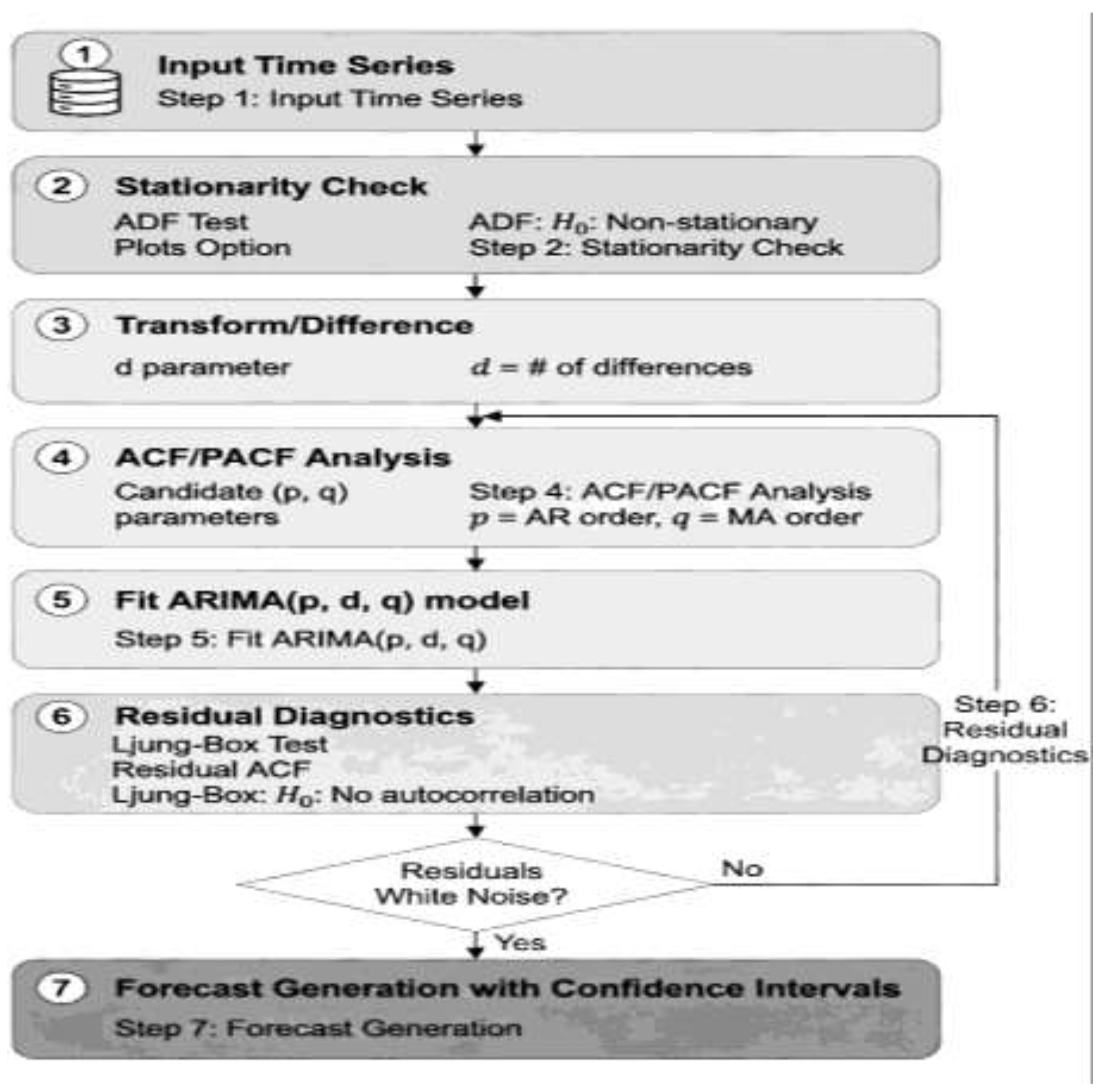
Figure 2.
LSTM Architecture.
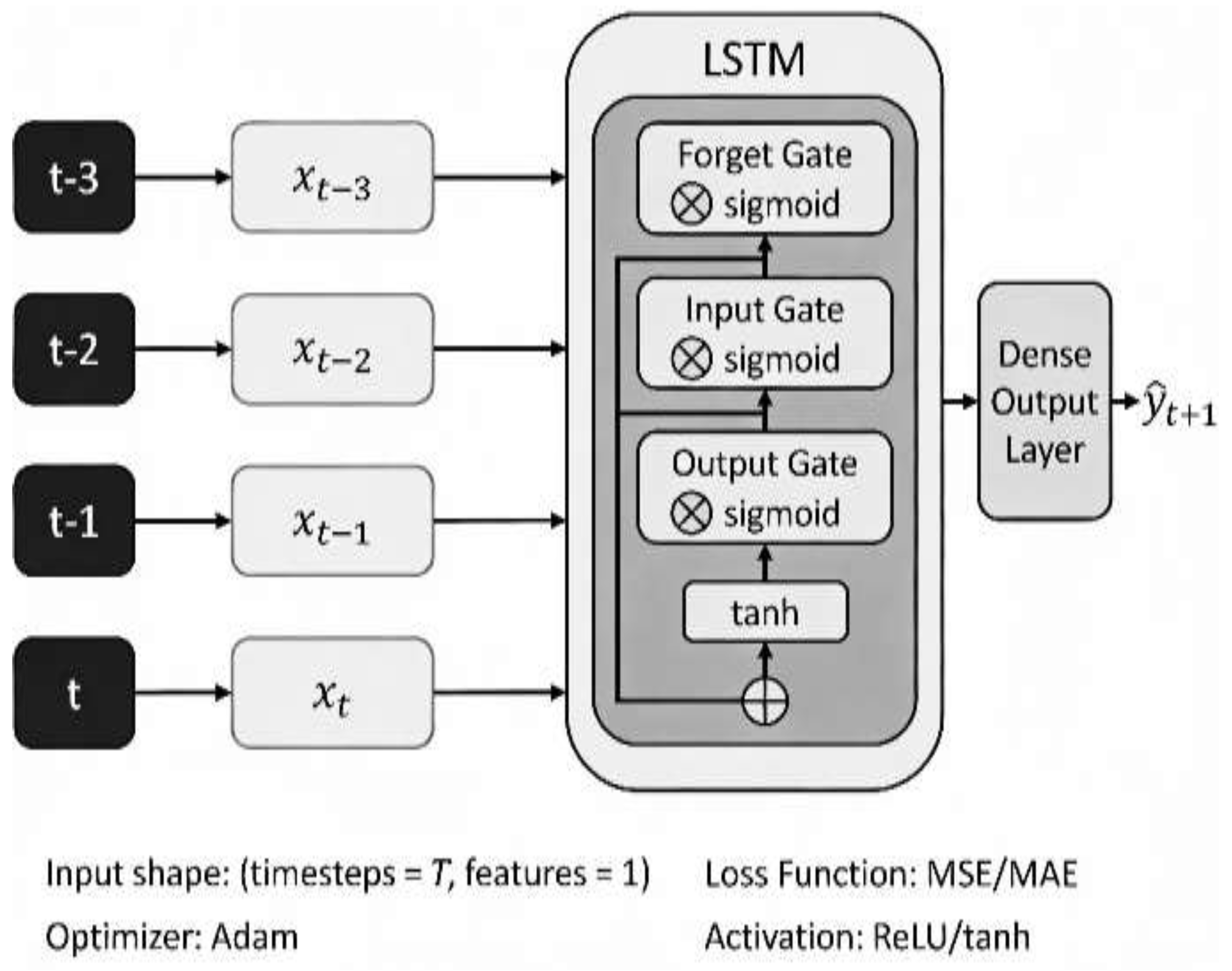
Figure 3.
Prophet Decomposition.
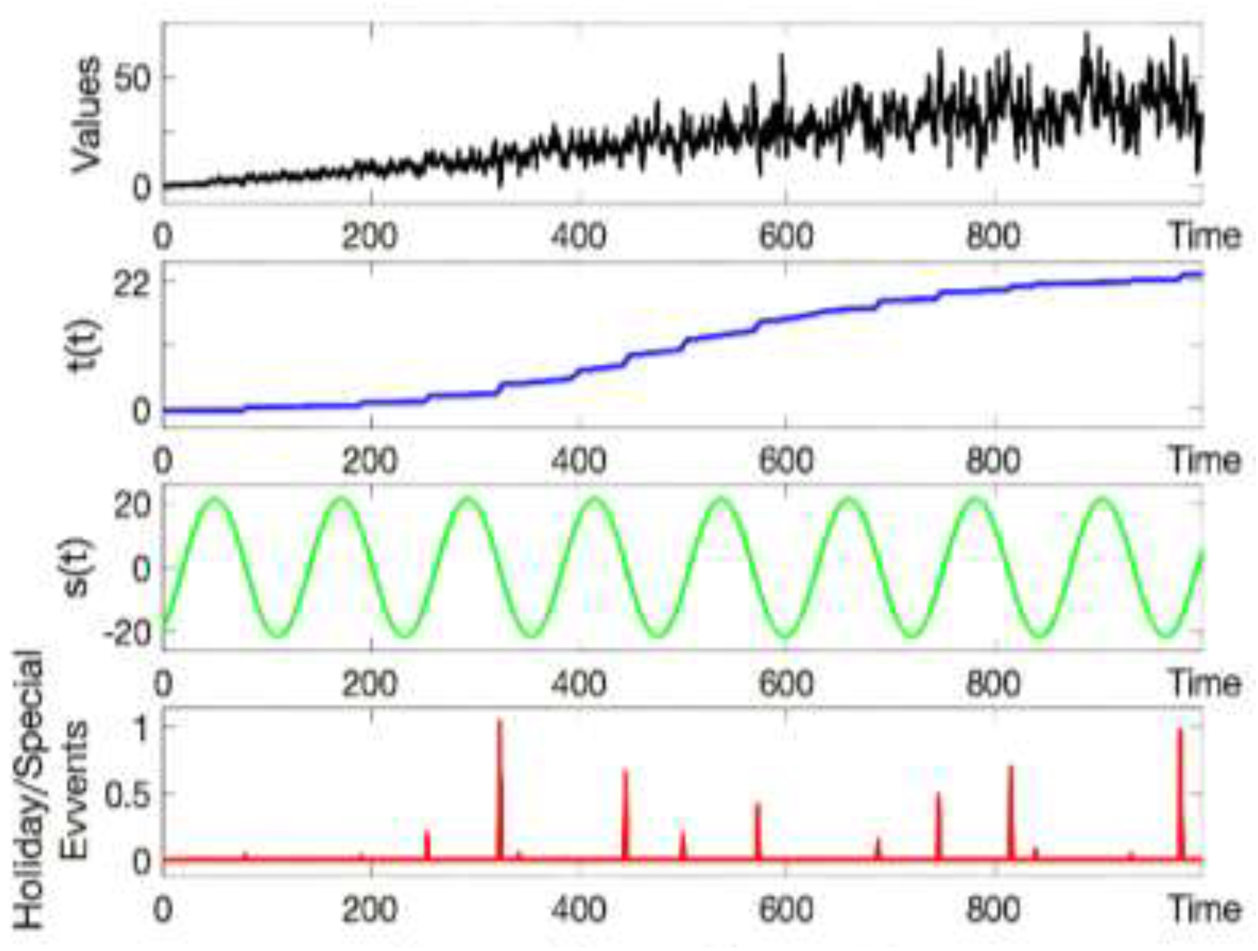
Figure 4.
Overall Research Workflow.
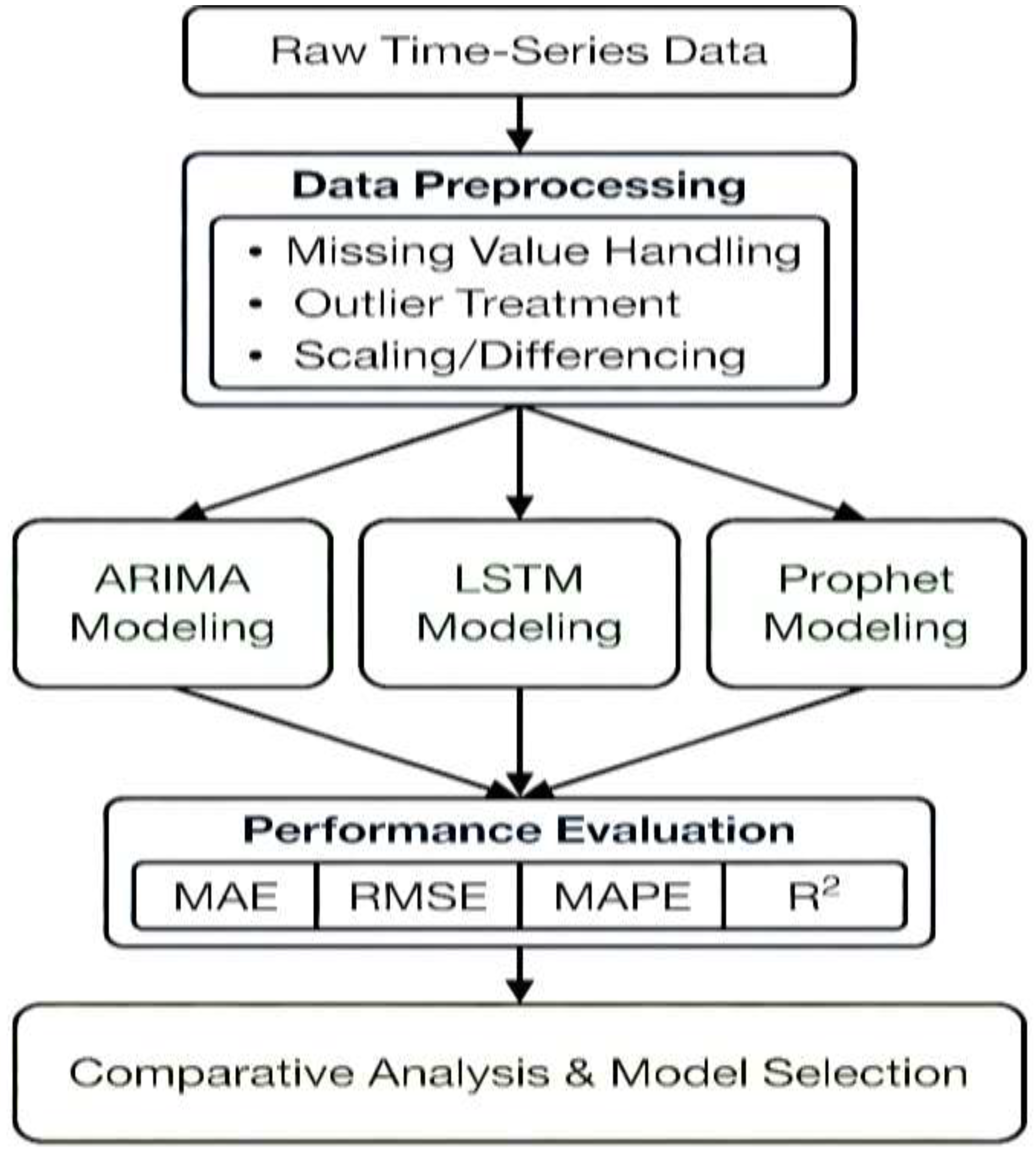
Figure 5.
Model Selection Decision Tree.
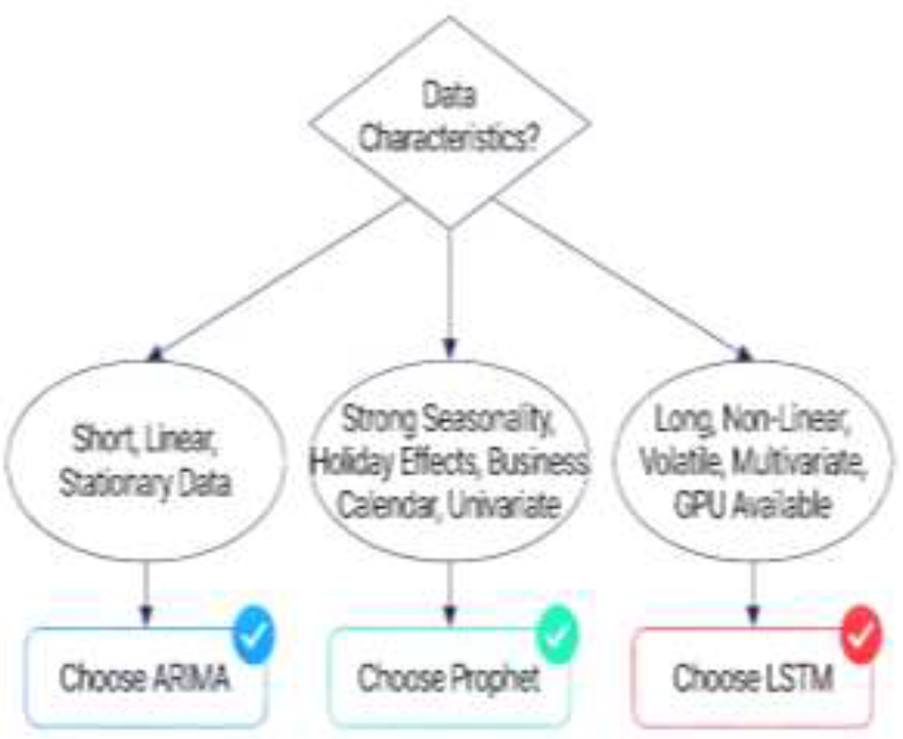
Figure 6.
Performance Comparison Chart.
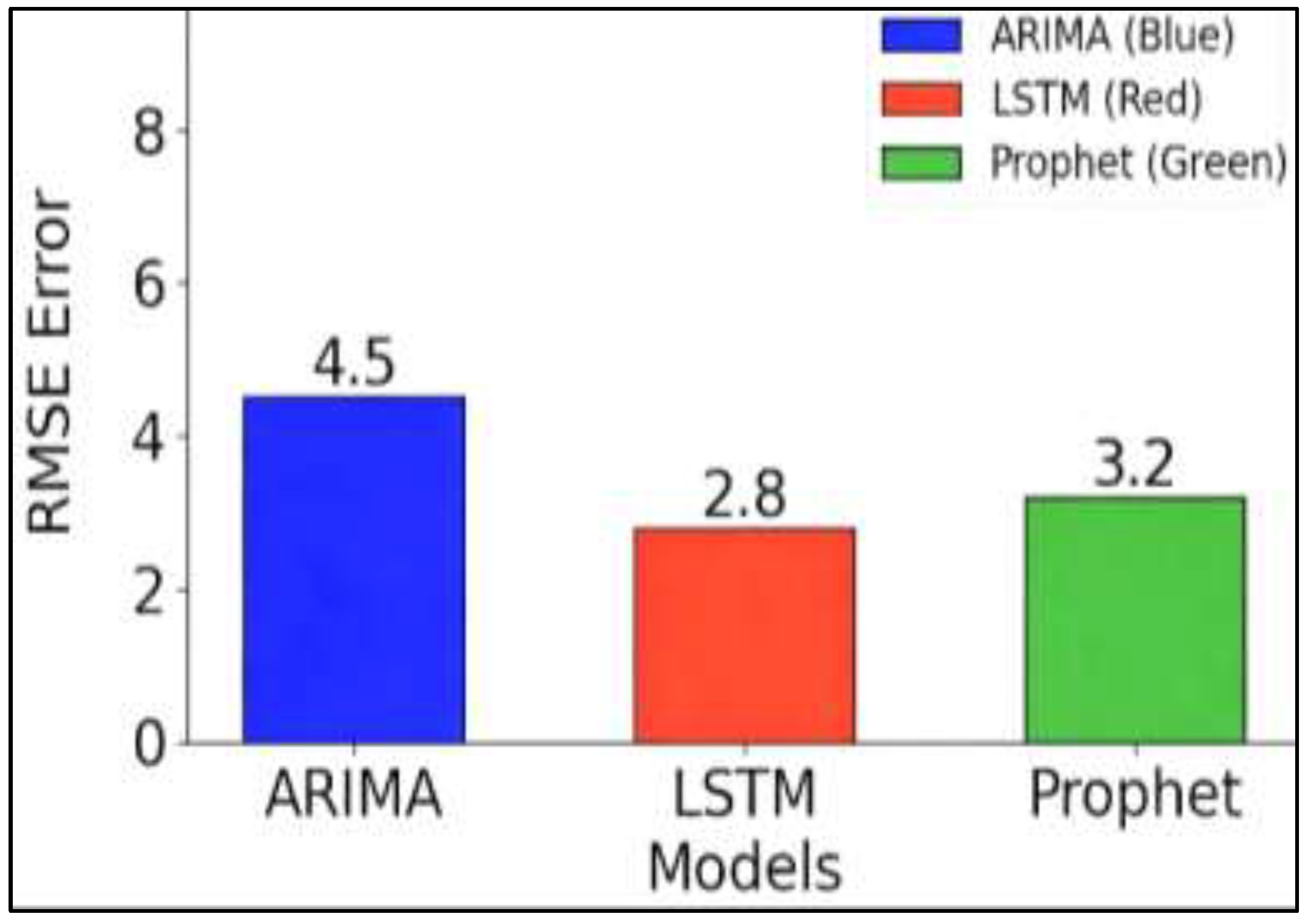

Table 1.
Comparative Performance Across Application Domains.
| Domain | ARIMA MAPE | LSTM MAPE | Prophet MAPE |
| Financial (Hourly) | 15.04% | 4.06% | 11.09% |
| Financial (Daily) | 3.20% | 6.60% | 6.30% |
| Energy (Renewable) | 8.5% | 3.2% | 5.8% |
| Traffic (Hourly) | 12.8% | 5.4% | 8.7% |
| Retail (Daily) | 8.6% | 9.2% | 7.4% |
| Healthcare (COVID-19) | 16.4% | 13.2% | 15.8% |
Table 2.
Model Performance Across Forecasting Horizons.
| Horizon | ARIMA Strength | LSTM Strength | Prophet Strength | Uncertainty |
| Hourly | Poor | Excellent | Weak | Very High |
| Daily | Good | Good | Excellent | High |
| Weekly | Excellent | Moderate | Good | Moderate |
| Monthly | Excellent | Poor | Good | Low |
Table 3.
Hybrid and Ensemble Model Performance Summary.
| Approach | Hybrid Type | MAPE Improvement | Computational Cost | Interpretability |
| ARIMA-LSTM | Decomposition | 5–20% | High | Moderate |
| Simple Ensemble | Averaging | 8–15% | Moderate | Moderate |
| Weighted Ensemble | Weighted avg | 10–18% | Moderate | Good |
| VMD-Deep Learning | Decomposition | 15–30% | Very High | Low |
Table 4.
Key Performance metrics across datasets.
| Model | RMSE | MAE | Training Time | Data Requirement | Interpretability |
|---|---|---|---|---|---|
| ARIMA | 3.11 | 2.34 | 1 minute | Low | High |
| LSTM | 2.48 | 1.92 | 30 minutes | High | Low |
| Prophet | 2.85 | 2.03 | 5 minutes | Moderate | High |
Disclaimer/Publisher’s Note: The statements, opinions and data contained in all publications are solely those of the individual author(s) and contributor(s) and not of MDPI and/or the editor(s). MDPI and/or the editor(s) disclaim responsibility for any injury to people or property resulting from any ideas, methods, instructions or products referred to in the content. |
© 2026 by the author. Licensee MDPI, Basel, Switzerland. This article is an open access article distributed under the terms and conditions of the Creative Commons Attribution (CC BY) license.
Copyright: This open access article is published under a Creative Commons CC BY 4.0 license, which permit the free download, distribution, and reuse, provided that the author and preprint are cited in any reuse.


