Submitted:
15 January 2026
Posted:
19 January 2026
You are already at the latest version
Abstract
This paper outlines a simple theoretical argument for the possibility of a quantum lin-ear Voigt effect at low temperatures in certain media in the optical regime. An unlikely starting point for the ensuing argument arises out of a long-established hydrodynamic Lorentz field-modified classical dispersion theory whose Voigt component of the opti-cal conductivity, when subjected to the Uncertainty Principle, results in a modified form in the quantum region. In contrast to its classical, second-order counterpart, this quantum Voigt conductivity is shown to have a (modular) linear field dependence
Keywords:
magneto-optics
; quantum magnetism
; linear magnetoresistance
1. Introduction
It seems hard to believe that, after more than a hundred years from the time of its discovery, there is still not much in the way of reliable published information on the Voigt effect in assorted magnetic materials, in the optical region, including doped semiconductors as well as transition metals, alloys and compounds. The Voigt effect is, of course, one of three major magneto-optical effects that are observable in a wide variety of materials, the other two being the better-known Faraday and Kerr effects. All three effects are interrelated, as can be demonstrated most effectively by examination of the elements of a gyroelectric optical conductivity tensor of the type shown, below, in Appendix A.
The Faraday and Kerr effects are both first-order effects in terms of magnetization/magnetic field dependence, of which the eigenfunctions are pairs of elliptically or circularly polarized wave functions of opposite helicity, depending on the disposition of the magnetic field in relation to the angle of incidence. The Voigt effect is a smaller magneto-optical phenomenon, observed in transmission or reflection, at normal incidence on surfaces with in-plane magnetic fields, a configuration in which the above-mentioned first-order effects vanish. A second-order effect, in terms of magnetization or external field dependence, it is characterized by orthogonal linear eigenfunctions, parallel to and orthogonal to the applied field. In the following, the Voigt component of the optical conductivity, derived from the above-mentioned hydrodynamic model is used, in conjunction with Heisenberg’s Uncertainty Principle, as a vehicle to investigate the nature of quantum fluctuations in the former, leading ultimately to an expression for the Voigt conductivity in the quantum region (defined later in Section 3).
Using the classical form for the magneto-optical component of the optical conductivity seems an unlikely starting point for an undertaking of this sort. The methodology is, however, straightforward and. when initially applied first, in Section 2, to zero-frequency extrapolations of the Kerr and Voigt conductivities, leads, respectively, to expressions for the quantum Hall effect (HE) and for the quantum Linear Magnetoresistance (LMR) in agreement with published work. The outcome of this procedure, when applied to the Voigt conductivity in the optical regime, strongly suggests the existence of a quantum linear Voigt effect at low temperatures. This would appear to suggest that quantum LMR is a special zero-frequency example of a more general phenomenon. Given the fairly limited amount of published material on this effect, (especially at very low temperatures), it is not surprising that experimental evidence, supporting the ideas set down in this paper, is exceedingly limited. One thing to be mindful of, here, is that the proposed model’s linear dependence, like its quantum LMR counterpart, is a modular one, meaning that it has, like the classical Voigt form, even field-dependent symmetry, making it, consequently, more difficult to differentiate from its classical quadratic counterpart. Some apparently supportive published experimental work is briefly evaluated in Section 5. A critical test for any magneto-optical theory is how well it describes, over a wide spectral range, the dispersion of key variables, such as the real and imaginary parts of the optical permittivity or conductivity. An equation consistent with Equation (4A) of the classical theory of Appendix A was, for example, shown to provide a reasonable description of the dispersion of the Kerr component of the optical permittivity in bulk samples of Fe and Co in the visible and near infra-red [2]. Corresponding dispersion measurements for the second-order Voigt effect, representing a much more stringent test of that theory, have not been as forthcoming but, based upon their own previously published experimental work [3,4,5], the present authors have recently shown [6] that Equations (4A) and (5A) describe, reasonably well, (see Figure 1 and Figure 2, respectively) the dispersion of the real and imaginary parts of the Voigt component of the optical conductivity in thin films of Fe and Co in the optical regime. Key parameters of this model (Appendix A) are the plasma (), cyclotron () and relaxation () angular frequencies.
The success of the model, particularly in its ability to depict the above 2nd order dispersion curves is quite remarkable given the very high scattering rates in transition metals at room temperature and the notion of cyclotron frequency being used to describe what is, in effect, skew-symmetric scattering caused by spin-orbit coupling. The model is, clearly, better-suited to doped semiconductors in the cryogenic temperature range where scattering is less disruptive, cyclotron motion is less of an artificial construct, where much of the current experimental interest in magneto-optics is concentrated and at which the analyses of Section 3 and Section 4, below, are directed.
The validity of this theory is further underlined, in the following two sections, by taking, respectively, the zero -frequency extrapolations of the Voigt () and Kerr () conductivities and, using the Heisenberg Uncertainty Principle and some simple reasoning, showing that, at temperatures well below the quantum limit, they lead to established forms for the quantum Hall Effect and quantum linear magnetoresistance.
Additionally, in Section 4, a similar argument is presented (along the lines of that used for the zero-frequency case), that, at optical frequencies, in the quantum region, there is reason to suppose that the Voigt component of the optical conductivity may not, necessarily, be a quadratic function of field, but, instead, of a functional form, reflecting a (modular) linear field dependence.
2. Fashioning an Expression for LMR Using the Zero-Frequency Limit
The linear field dependence of magneto-resistance in a variety of conducting media has, for decades, been a topic of considerable and sustained scientific interest [7,8,9,10,11,12,13,14]. As Falicov and Smith [14] have articulated, published explanations of the origins of this linear behaviour, all highly sophisticated, reveal the following dichotomy. On the one hand there are analyses based largely on morphology [9,10]. Here, the disorder of the metal is the dominant theme, the models being framed in terms of discontinuities, microstructure, and so on. On the other hand, a separate body of literature appears to favour explanations based upon intrinsic properties of the materials in question. That body, itself, sub-divides further into two sets, one focusing on common, but atypical, metallic band features such as (strong) spin correlations, (small) energy gaps and ground states defined by spin density waves [11,12]. The other set concentrates on localized anomalies in the Fermi surface leading to ‘hot spots’ [13] and related issues [14]. All of these models are impressive works, but, for the most part, rather complex. In contrast, the observed transition from the ‘normal’ quadratic MR effect into a linear form, below the quantum limit, is now described much more simply, but, at the same time, in a form consistent with the existing body of knowledge.
This section of the paper attempts, by a rather unorthodox approach, to construct a simple model for LMR, in conducting media, below the quantum limit. The method employed is that of taking phenomenological expressions for the leading diagonal elements of the gyroelectric tensor of Appendix A and calculating the uncertainty in those elements in terms of quantum fluctuations in both the cyclotron and carrier relaxation frequencies.
This leads to fundamental fluctuations in a part of the resistivity, quadratic in magnetic field, normally associated with conventional magnetoresistance. At an appropriate point, Heisenberg’s uncertainty principle is invoked, resulting in a simple expression for LMR that is fully in agreement with published experimental work [15,16,17]. A rather similar approach has already been used successfully in the calculation of ballistic conductance in nanowires [18].
It should be noted that the conductivity tensor in question is based solely on considerations of intrinsic symmetry [1], meaning that morphological questions are not dealt with here. That does not, of course, imply that the latter are unimportant; quite the opposite, in fact. Both first and second-order galvanomagnetic effects can be shown to be crucially dependent on crystal symmetry [19]. Such considerations, however, are beyond the scope of this study and are not considered further.
3. Outline of the Method
The analysis summarized in Appendix A results in a (zero frequency) gyroelectric conductivity tensor (see Equation (7A)) with the leading diagonal elements, given, at zero frequency, by
where is the plasma frequency,
is defined as , where τ’ is a relaxation time dominated by cyclotron scattering,
is the (angular) cyclotron frequency, B is the applied magnetic field, and is the cyclotron mass of the carrier [20].
Inversion of the gyroelectric tensor (7A) allows a determination of the leading diagonal element, ρxx, of the resistivity tensor [24].
If the condition, (i.e., ωcτ ≤ 1), is applied, σxy, in the denominator may be safely ignored and
The diagonal resistivity, , is now seen to be
It should be noted that
- (i)
- ρ is not the zero field resistivity. It is, actually, the resistivity of the sample when the applied field is in the z-direction (i.e., ).
- (ii)
- The zero field resistivity, ρo , arises from the solution of (1A) for the case Bz = 0.where ωo = 1/τo is the carrier relaxation frequency in zero field.
For a fixed (z-direction, say) of current flow, orthogonal fields applied in the x- and z- directions result in the qπuadratic field-dependent resistivity differential, . It should also be noted here that (see Appendix B), in modest aππpplied magnetic fields and over a wide range of temperatures, the magnetoresistive component of Equation (3), , leads directly to the familiar quadratic field-dependent equation, Equation (2B)
where is the carrier mobility in zero magnetic field, and to the familiar Drude expression for the magnetoresistance ratio (Equation (3B)).
By contrast, LMR may be regarded as a fundamental fluctuation in this quantity in the quantum limit [18].
The resulting uncertainty in , labelled here as , can, therefore, be shown to be
where the Δ prefix on the right side of (5) refers to the uncertainty in that expression. It follows that
The modulus sign, bracketting ωc, simply means that the magnitude of the uncertainty is independent of the polarity of the z-directed magnetic field, B. If the right side of Equation (6) is multiplied, top and bottom, by h/2π, then
Here, , represents the uncertainty in either the spin-up or spin-down electrons [21], meaning that the overall uncertainty in the resistivity is exactly half of that shown in Equation (7). It is generally accepted that, for all but the very highest fields, only the first Landau level is attainable by carriers in the quantum region [14]. The quantity may, therefore, be viewed as an uncertainty in the energy gap between the zeroth (lowest) Landau level and the ground state energy caused by (say) spin-density or charge-density fluctuations in the latter [9,10]. Likewise, represents uncertainty in the cyclotron scattering relaxation time. Equation (7) may, therefore, be re-expressed as
Combining Equations (4) and (7) results in a magnetoresistance ratio of the form
This equation is identical to an empirical relationship fashioned by Johnson et al. [17] from LMR data on MnAs-GaAs composites and one which appears to provide an explicit form for Kohler’s Rule [23] in doped semiconducting systems.
Clearly, under certain conditions, the classical quadratic form of MR transitions into the quantum linear form, at which point it follows from Equations (2B) and (8) that:
I.e. the transition takes place when , or
Xin et al. [24] have shown that where C (~1) is an activation constant.
It follows that LMR can occur when which seems to be in rough agreement with earlier definitions of the quantum regime for LMR. It is shown in Appendix C that a consequence of the Heisenberg Uncertainty Principle (HUP) is that the product of the uncertainties in B and in
Taking the traditional form of in Equation (2B) and assigning an uncertainty in it (in the manner described for Equation (6)) as well as the corresponding uncertainties in B and gives
resulting in:
which is consistent with the LMR form of Equation (8). The factor of 2 disappearing when spin-up/spin-down is considered.
4. A Simple Approach to the Quantum Hall Effect
It may also be shown that, although not the main thrust of this paper, the same basic approach may be used with the off-diagonal Hall conductivity, in Equation (8A),for, say, a two-dimensional mesoscopic sample. The off-diagonal resistivity, ρxy , can easily be shown, in the classical region, to be
i.e.,
where ωs is a relaxation frequency limited, among other things, by surface scattering, and ρo is the resistivity of the mesoscopic sample in zero field.
Evaluating the uncertainty in this quantity below the quantum limit, with ωs equated to 2π/τs , results in
Once again, the electron spin-up, spin-down dichotomy means that the Hall resistance, in the quantum region, is half of the ballistic resistance of a mesoscopic rectangular strip (along the axis of current flow). In other words, the Hall resistance is given by von Klitzing’s constant (h/e2). the expected result for the integral quantum Hall effect [16].
It should be noted here that the classical conductivity tensor, in the form shown in Appendix A, and based solely upon considerations of intrinsic symmetry, is also well-suited to highly disordered systems in which the influence of crystal symmetry is diminished. Composites with non-conducting phases, thanks to effective medium theory, do not present serious difficulty in fashioning a conductivity tensor in the manner of (7A), provided that the conducting phase is comfortably below the percolation threshold.
5. Quantum Aspects of the Voigt Conductivity in the Optical Regime
Given the ability of this model to provide correct forms for the quantum HE and the quantum LMR, the question then arises: what is the form of the magneto-optical Voigt conductivity, in semiconductors, in the optical region at temperature ? To obtain the answer to this, the same procedure used to determine uncertainties, already used in Section 3, is now applied to Equation (4A), as follows
An examination of the Voigt component of Equation (4A) upon applying the same uncertainty procedures as used for the zero frequency expressions of Section 3 are dealt with in the following manner. When the electric field vector of the incident light wave is aligned in the z-direction, the material is magneto-optically inactive and the relative permittivity is given by Equations (2A) and (3A)
where is effectively unity. By contrast, when the electric field vector is oriented in either the x- or y- directions, the relative permittivity, under normal circumstances, is given by Equations (2A) and (3A)
The Voigt effect is driven by the permittivity difference In the cryogenic region, uncertainty in the free electron component of is therefore given by
Since ωc << ω, ωr, Eq (14) can be expressed as
When spin up-spin down considerations are taken, as before, the expectation of the Voigt permittivity becomes:
Note that a factor of 2 applies to the first term of equation (15) as well, meaning that, (along with ), it cancels the relative permittivity of the z-direction. Equating this uncertainty to quantum transitions to the lowest Landau level [11], the quantum Voigt permittivity, using Equation (16), becomes
and the Voigt conductivity becomes proportional to the modulus of the applied field It is easily shown that the Voigt rotation is proportional to both in reflection and in transmission, if the Voigt conductivity is similarly dependent.
It should be noted that, in this equation, reduces to a form identical to Equation (9) as the frequency tends to zero. It is likely to exist only at the lowest temperatures of the quantum region and, like its zero-frequency counterpart, most likely brought about by transitions from the ground state to low-lying Landau levels [11]. Like the classical quadratic Voigt effect, this putative quantum version has even symmetry, meaning that it may well have gone unrecognized and attributed to lack of field saturation or other experimental considerations.
Figure 3 shows the real and Figure 4 the imaginary part of the quantum Voigt conductivity, plotted in terms of the frequency of illumination, following Equation (18). The curves show dispersion in the vicinity of . Given the typical relaxation frequencies of semiconductors at low temperature, it would seem to suggest that this putative quantum effect could be large in the far infra-red and terahertz regions. The analysis of Appendix A would seem to suggest one possible reason for the comparatively large Voigt effect at low temperatures. In the conventional quadratic case, the optical Voigt permittivity is given approximately by
By contrast, Equation (17) gives the corresponding quantum Voigt permittivity. Given that, typically, these two equations may well explain some of the anomalously large, low-temperature Voigt rotations.
6. Experimental Evidence
Recent experimental evidence supporting the above-mentioned arguments is lacking. It may be instructive, however, to revisit a 1991 experimental paper [22] dealing with giant Voigt effects in diluted magnetic semiconductors, namely alloys of CdMnTe. That paper shows two plots of Voigt rotation versus the square of the applied field, one for a sample at a temperature of 20K, one at a temperature of 5K and both subjected to magnetic fields in excess of 5T.
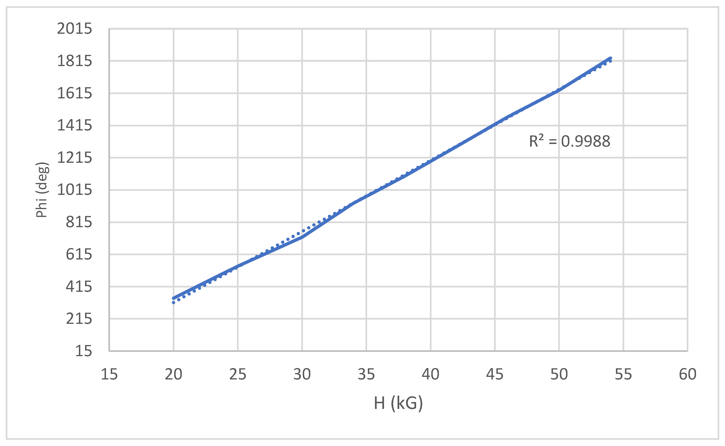
Both plots show good adherence to the classical quadratic Voigt field dependence at lower applied fields (0 ≤ 2T) but no such agreement at higher fields. Eunsoon et al. [22] ascribe the reason for this on saturation of the magnetization at a relatively low value of applied field. Those plots are now reproduced, below, in Figure 5 and Figure 6, respectively, only this time the rotations are shown, for higher fields only and as functions of magnetic field, H. In both plots, the Voigt rotations show a clear linear dependence on magnetic field with no evidence whatsoever of saturation.
It would seem, therefore, that, at modest values of applied field, the conventional quadratic Voigt effect is observed. At higher values of applied field, magnetization is not a factor and the quantum linear Voigt effect, brought about by transitions to the lowest-lying (degenerate) Landau level, generated by high applied fields, displacing the classical form, but only when the applied field is high enough to achieve the quantum transition and only when the temperature is low enough to suppress thermal disruption. At fields of nearly 6T, in a manner reminiscent of quantum LMR, there is no evidence of saturation of rotation. In their paper, Eunsoon et al. [22] also pronounce the requirement for obtaining giant Voigt effects as being one of subjecting magnetic semiconductors to cryogenic temperatures and very high fields, a condition consistent with arguments made by the present authors for the realization of a quantum linear Voigt effect. The comparatively large quantum Voigt permittivity of Equation (17), compared to that of the traditional Voigt effect (Equation (19)), reinforces this argument.
7. Conclusions
This paper has attempted to show that the Voigt effect might be a little more complicated in the cryogenic region than previously imagined and that the second-order magnetization/magnetic field dependence may not always be valid there. One obvious limitation of the analysis in Appendix A is that the polarization of the lattice is not considered. Clearly, in a compensated system, involving excitons and holes, the uncertainty in optical conductivity leading to Equation (18) will be further enhanced by an amount dependent on the hole mobility at optical frequencies. Nevertheless, the modular linear dependence on magnetic field will persist.
A corollary to all of this is that quantum linear magnetoresistance may simply be a zero-frequency component of a more general phenomenon. Significant supportive experimental evidence is lacking, of course, but the even field symmetry caused by a modular linear field-dependent relationship might well have, hitherto, caused the effect to ‘hide in plain sight’ from even the most experienced investigators..
Acknowledgments
The authors would like to take this opportunity to dedicate this paper to the memories of Professors Paul H Lissberger of the Queen’s University and Roy Carey of Coventry University, both of whom passed away recently and who were major figures in the field of magneto-optics in the second half of the 20th century. Lissberger, a distinguished graduate of the University of Manchester, was widely regarded as a leading world authority in the optics and magneto-optics of thin film multilayers. Professor Carey, a distinguished graduate of L. F. Bates’ renowned magnetism group at Nottingham University, was one of the first in the United Kingdom to investigate the Voigt Effect. One of the present authors (MRP) is indebted to the University of Salford and to the University of Alabama for providing, in the distant past, support that helped generate the origins of the work described above.
Appendix A. Hydrodynamic Model of the General Conductivity Tensor in Semiconductors
The basis of this model, given only in outline, here, is classical dispersion theory with the focus on materials with a single dominant carrier [9] and with the polarization of those carriers and all other bound charges considered separately. The influence of the latter is simply embodied in a non-dispersive (real) component of the (absolute) permittivity, εB , associated directly with the lattice, with essentially no impact on the following analysis. The focus is completely on the free carriers, of number density, n, which move with velocity, v, when exposed to a local electric field E = Eo exp(-iωt) of angular frequency, ω. If an external dc magnetic induction field, B = [0,0,Bz] is applied, then the equation of motion is
(for the case where the dominant carrier is the electron), where e is the magnitude of the electronic charge, m* the cyclotron effective mass and ωr is an angular carrier relaxation in frequency heavily influenced by cyclotron precession. The solution of (1A) has been described in detail previously [1] and is only summarized here. The complex relative permittivity tensor is written as
where κB is the relative permittivity of bound charge associated with the lattice, is the (angular) plasma frequency, and . Here, , and .is the cyclotron frequency of the carriers in the presence of the applied external magnetic field.
Explicit forms for the leading diagonal elements, εxx, εyy, in terms of cyclotron frequency (or of applied magnetic field) are easily obtained from the above tensor equation. Since those elements are complex, the imaginary parts (multiplied by -iωεo) lead directly to a corresponding conductivity tensor. For example
Then for C << A, so that is the Voigt contribution to the diagonal component
Therefore, the real and imaginary parts of the Voigt conductivity are
By similar reasoning, the off-diagonal elements of the above tensor can be similarly expressed, this time as an explicit first-order function of ωc.
It is a simple matter to express (3A) in terms of its real and imaginary parts as follows
where
The zero frequency gyroelectric contribution to this permittivity, and ultimately, the optical conductivity, is isolated, in stages, by a rather tedious but straightforward calculation, resulting in real and imaginary zero frequency conductivities:
where
Appendix B
From Equation (3), the conventional quadratic MR resistivity is
The damping term in Equation (1A), , can be re-expressed in terms of the carrier mobility in zero magnetic field, μc, as
Substituting and in Equation (1B) and cancellation, gives
Appendix C
The energy/time version of the Heisenberg Uncertainty Principle (HUP) used here is
In the context of the present paper:
is a corollary of the HUP.
As a systematic check on the LMR result of Equation (2B), for low field, conventional MR can be assigned an uncertainty along the lines of the LMB evaluation of Section 2, as follows
Using the above corollary, Equation (1C), is transformed as follows
The uncertainty is halved when spin-up/spin-down considerations are applied and the LMB is once again:
References
- Lissberger, P.N.; Parker, M.R. “Theory of the Voigt effect in gyroelectric media”. Int. J. Magnetism 1971, vol 1, 209–218. [Google Scholar]
- Krinchik, G. S.; Artemiev, V. A. Sov. Phys. J. E. T. P. 1968, Vol. 26, 1080–1083.
- Birss, R.R. Collings, N. Parker, M.R. “Dispersion of the Voigt effect in thin iron films”, Physics Letters A, January 27, 1975Volume: 51, Issue: 1, , Page: 13.
- Birss, R.R. Collings, N. Parker, M.R. “Dispersion of the linear magnetic birefringence in transition metal films”, Physica B & C, v.86-88 B+C pt.3, 1977, 1203-4.
- Collings, N. Birss, R. Parker, M. “Resonance optical absorption in iron in the visible region,” IEEE Transactions on Magnetics, vol. 17, no. 6, 1981,pp. 3235-3237.
- Collings, N. and Parker , M. R., ,Proc. Joint IOP/ITN MagnEFi, 28-29 Oct 2021.
- Kapitza, P L. Proc. R. Soc., A 119 1928, 358–443.
- Abrikosov, A A. Sov. Phys.-JETP, 29 1969, 746–753.
- Amundsen, T; Jerstad P, J. Low Temp. Phys., 15 1974, 459–471. [CrossRef]
- Pippard, A B. Phil. Trans. R. Soc., 291 1979, 561–598.5.
- O’Keefe, P M; Goddard, W A. Phys. Rev. Lett., 23 1969, 300. [CrossRef]
- Overhauser, A W. Phys. Rev. B, 3 1971, 3173. [CrossRef]
- Young, R A. Phys. Rev., 175 1968, 813. [CrossRef]
- Falicov, L M; Smith, H. Phys. Rev. Lett., 29 1972, 124–127. [CrossRef]
- Hu, J; Rosenbaum, T F. Nature Materials, 7 2008, 697–700. [CrossRef]
- Xu, R; Husmann, A; Rosenbaum, T F; Saboungi, M-L; Enderby, J E; Littlewood, P B. Nature, 390 1997, 57. [CrossRef]
- Johnson et al. Phys. Rev. B, 82 2010, 085202-1-085202-4.
- Batra, I P. Solid State Comm., 124 2002, 463–467. [CrossRef]
- Birss R R, ‘Symmetry and Magnetism’, (North-Holland, Amsterdam), 1966.
- Ziman, J. M, ‘Theory of Solids’, 2nd ed.; Cambridge Univ. Press, 1992; pp. 304–309. [Google Scholar]
- Abrikosov, A A. Phys. Rev. B, 58 1998, 2788–2794. [CrossRef]
- Eunsoon Oh, D.U. Bartholomew, AK. Ramdas, J.K. Furdyna, and U. Debska. Phys. Rev. B 44 1991, 10551. [CrossRef] [PubMed]
- M. Kohler, Zur magnetischen widerstandsänderung reiner metalle. Ann. Phys. 32 1938, 211–218.
- Xin, N.; Lourembam, J.; Kumaravadivel, P.; et al. Giant magnetoresistance of Dirac plasma in high-mobility graphene. Nature 616 2023, 270–274. [Google Scholar] [CrossRef] [PubMed]
Figure 1.
The real Voigt conductivity of Iron versus the frequency of the illumination.
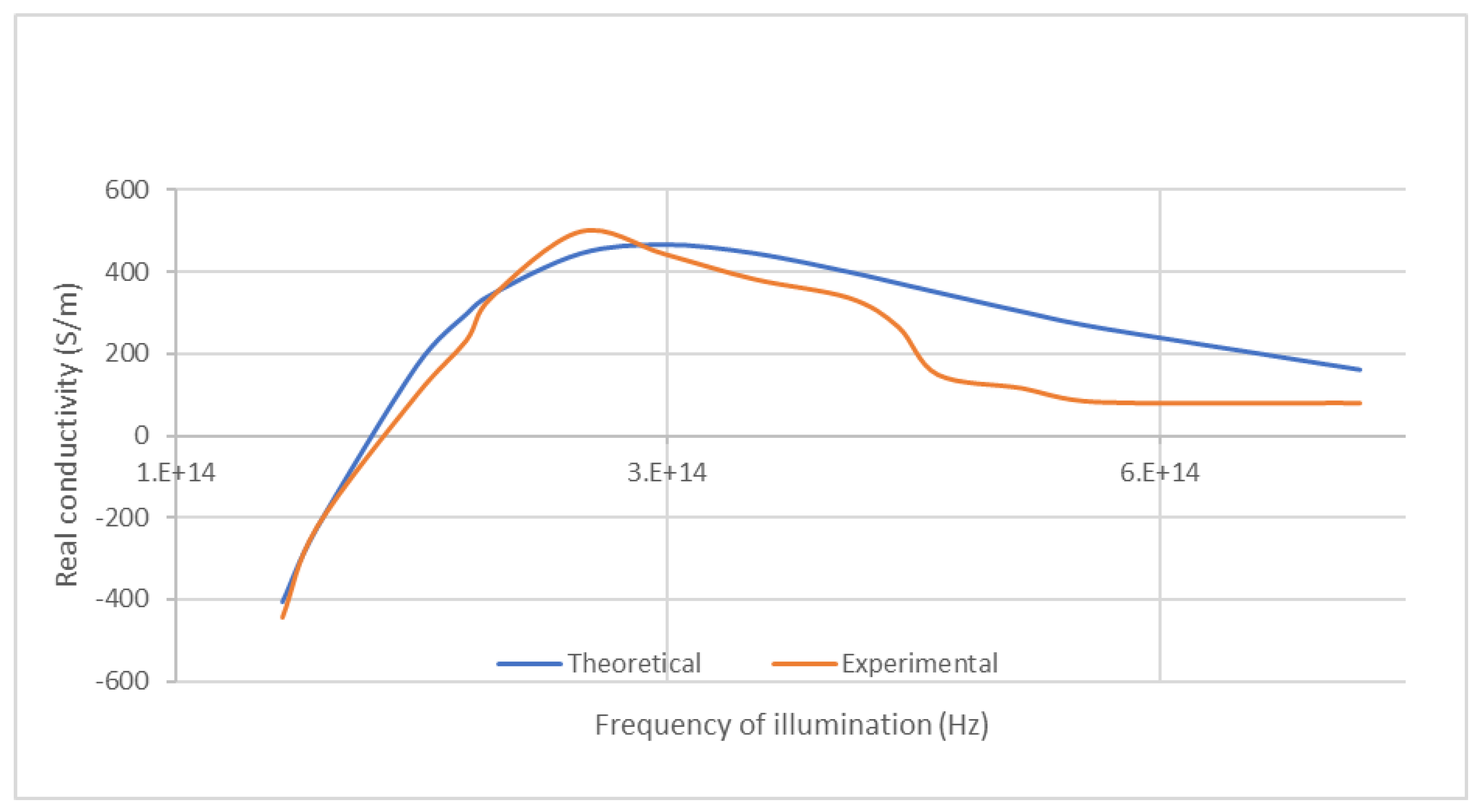
Figure 2.
The imaginary Voigt conductivity of Iron versus the frequency of the illumination.
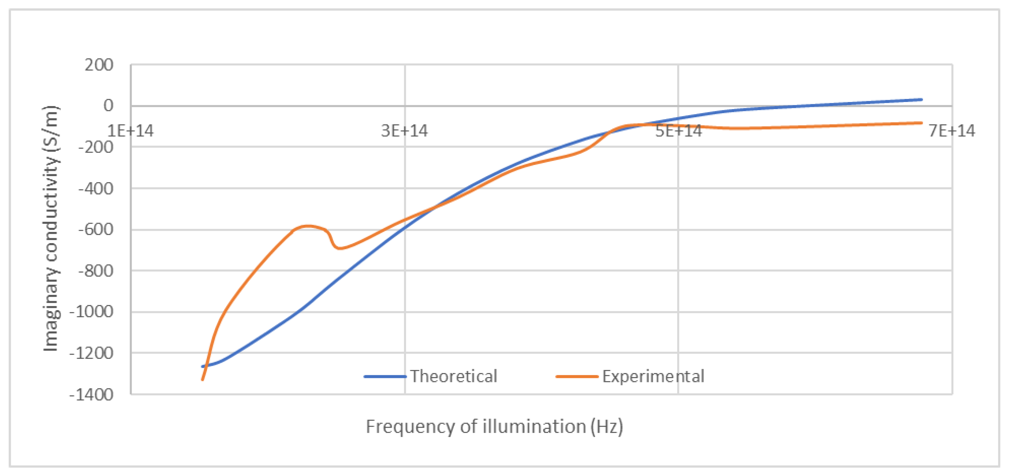
Figure 3.
Plot of real part of the quantum Voigt conductivity versus frequency of illumination in equation (18).
Figure 3.
Plot of real part of the quantum Voigt conductivity versus frequency of illumination in equation (18).
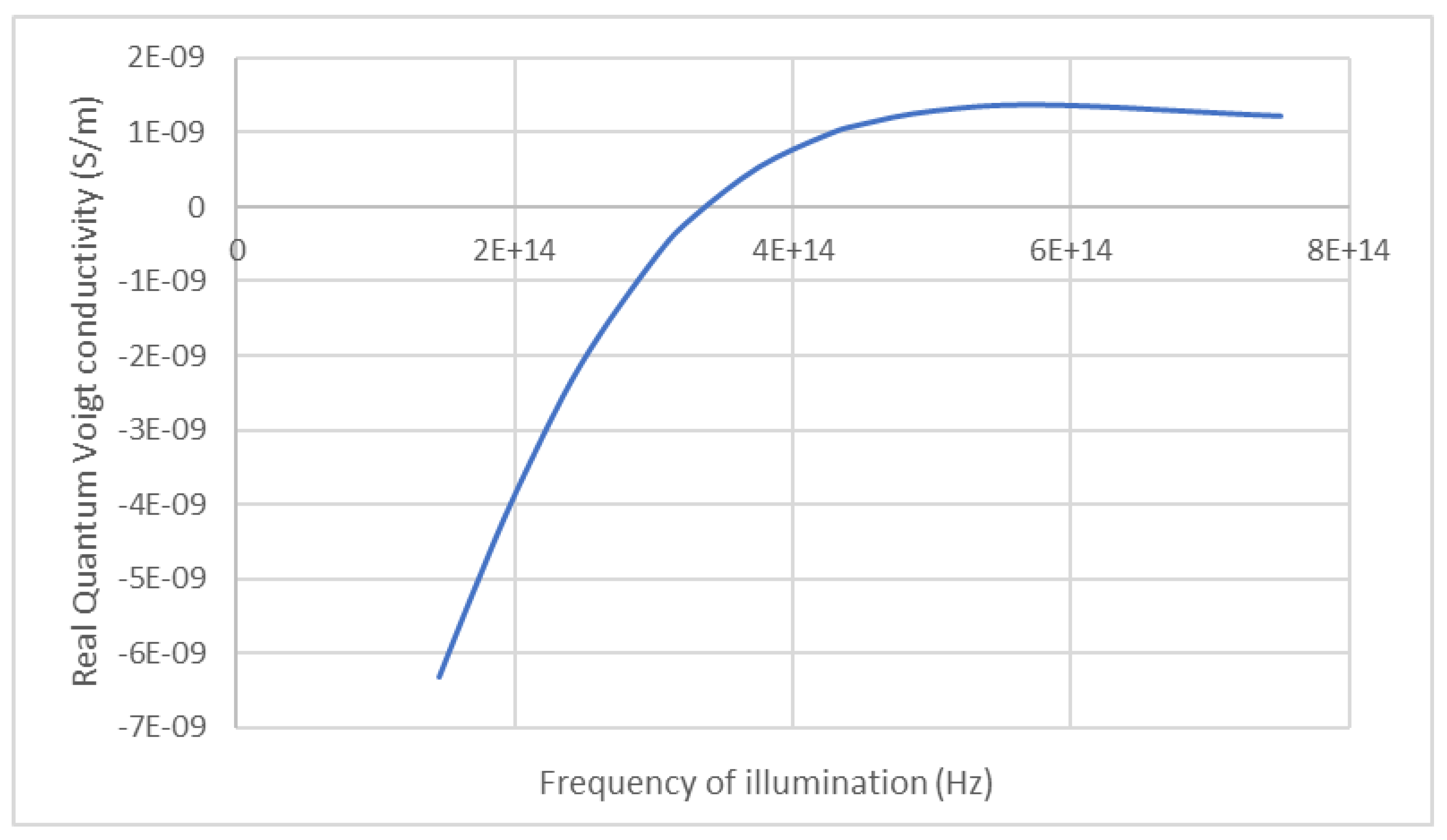
Figure 4.
Plot of imaginary part of the quantum Voigt conductivity versus frequency of illumination in equation (18).
Figure 4.
Plot of imaginary part of the quantum Voigt conductivity versus frequency of illumination in equation (18).
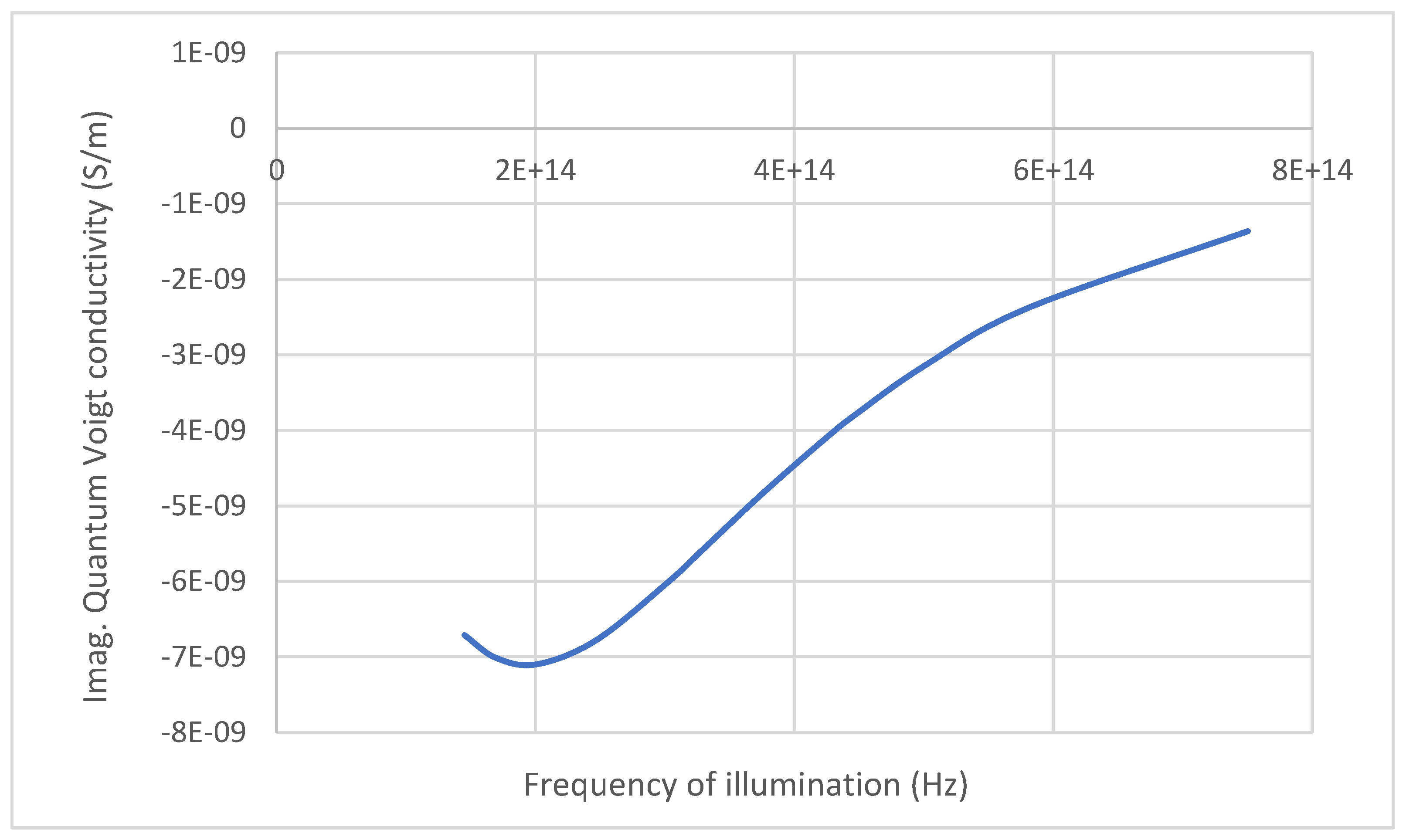
Figure 5.
Reproduction of Eunsoon et al.’s plot [22] of giant Voigt rotation of CdxMn1-xTe (x=0.65) at T=20K.
Figure 5.
Reproduction of Eunsoon et al.’s plot [22] of giant Voigt rotation of CdxMn1-xTe (x=0.65) at T=20K.
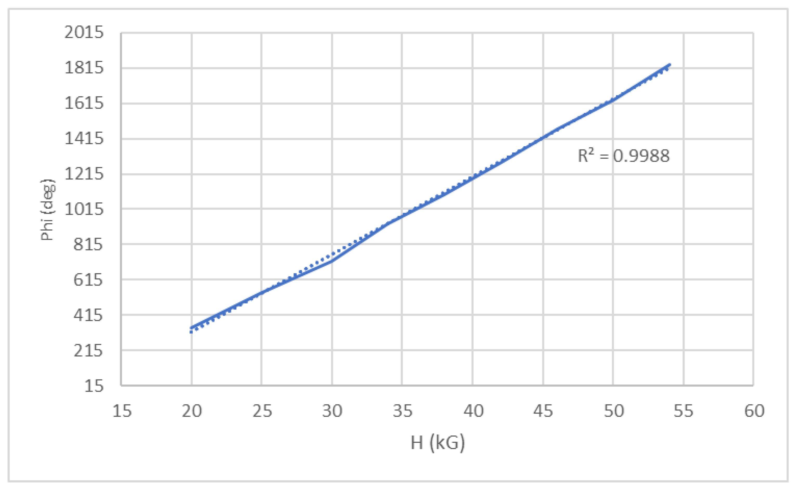
Figure 6.
Reproduction of Eunsoon et al.’s plot [22] of giant Voigt rotation of CdxMn1-xTe (x=0.18) at T=5K.
Figure 6.
Reproduction of Eunsoon et al.’s plot [22] of giant Voigt rotation of CdxMn1-xTe (x=0.18) at T=5K.
Disclaimer/Publisher’s Note: The statements, opinions and data contained in all publications are solely those of the individual author(s) and contributor(s) and not of MDPI and/or the editor(s). MDPI and/or the editor(s) disclaim responsibility for any injury to people or property resulting from any ideas, methods, instructions or products referred to in the content. |
© 2026 by the authors. Licensee MDPI, Basel, Switzerland. This article is an open access article distributed under the terms and conditions of the Creative Commons Attribution (CC BY) license (http://creativecommons.org/licenses/by/4.0/).
Copyright: This open access article is published under a Creative Commons CC BY 4.0 license, which permit the free download, distribution, and reuse, provided that the author and preprint are cited in any reuse.


