
Submitted:
12 January 2026
Posted:
14 January 2026
You are already at the latest version
Abstract
In order to solve the problems of insufficient privacy protection and limited sharing of industrial Internet security situation data,a situation element extraction model integrating federated learning and deep learning was proposed. This model integrates deep residual networks, bidirectional long short-term memory networks, and Transformer architecture,which extract features from network security situation data from multiple dimensions such as local features, temporal characteristics, and global correlations, and establish a situation element extraction model. Under the federated learning architecture,each participant performs data processing and model updates locally,transmitting model parameters through security mechanisms to reduce unnecessary data sharing and flow. The experimental results show that this method further improves the situation element extraction performance while protecting data privacy.
Keywords:
industrial internet
; deep learning
; federated learning
; situation element extraction
1. Introduction
With the rapid development of Industrial Internet, network security has become an important issue to ensure the stable operation of industrial systems. Industrial Internet involves not only the transmission and processing of a large number of sensitive data, but also the complex network environment and a variety of security threats. Therefore, how to effectively carry out network security situation awareness under the premise of protecting data privacy has become one of the hot spots of current research. Security situation awareness can monitor and evaluate the network security status in real time through the comprehensive analysis of network traffic and device behavior, the extraction of security situation elements is to extract representative features from massive data for subsequent threat detection and defense decision-making. However, the existing security situation element extraction methods still have obvious shortcomings in data privacy protection, feature extraction ability and model generalization. Therefore, an efficient situation element extraction model [2] can not only improve the detection ability of potential security threats, but also protect data privacy in a multi-source data environment [3] and avoid data leakage, it is of great significance to build a trusted industrial internet security system.
At present, a large number of studies have been devoted to the extraction and modeling of security situation elements, including deep learning methods, traditional machine learning methods and methods based on federated learning. The deep learning method automatically extracts complex network traffic features through convolutional neural network (CNN) and recurrent neural network (RNN), which has strong feature expression ability. However, deep learning models usually rely on a training, resulting in poor generalization ability of the model [4]. Traditional machine learning methods, such as support vector machine (SVM), random forest (RF), and K-nearest neighbor (KNN), perform well on small-scale datasets, but in a complex industrial internet environment, the performance of traditional machine learning methods is poor, often lack sufficient flexibility and adaptability [6]. With the increasing demand for data privacy protection, Federated Learning, as a new distributed Learning framework, has been gradually applied to the field of network security. Federated learning can effectively protect data privacy by co-training the global model without sharing the original data. Although the existing research combines federated learning with deep learning, such as the intrusion detection system based on federated learning [7], however, these methods still have some limitations in multi-dimensional feature fusion, complex environment adaptability and model generalization ability.
Aiming at the shortcomings of existing research, this paper proposes a security situation element extraction model FL-RBTNet that integrates federated learning and deep learning. The model combines a deep residual network (ResNet), a bidirectional long-short-term memory network (BILSTM), and a Transformer architecture, and the proposed model is applied to a real-world dataset, important information in network security data is extracted from multiple dimensions (local features, temporal characteristics and global context), which significantly improves the feature extraction ability. By adopting the Federated Learning Framework, FL-RBTNet not only guarantees data privacy, but also improves the generalization ability and adaptability of the model through distributed training [8]. In addition, FL-RBTNet can simultaneously perform deep feature modeling from multiple perspectives such as local features, temporal features, and global context information, which effectively enhances the model's ability to identify and classify complex network traffic.
The experimental results show that FL-RBTNet achieves excellent performance on KDD Cup99, SCADA2014, and ToN-IoT2021 datasets, especially on metrics such as precision, recall, and F 1-score, which can be used to improve the performance of FL-RBTNet, compared with traditional methods and existing deep learning models, fl-rbtnet has significant advantages. Through these experiments, this paper verifies that FL-RBTNet effectively solves the problems of data privacy protection and insufficient generalization ability of the model while improving the extraction ability of security situation elements, it provides a feasible solution for industrial internet security.
2. Related Work
In this section, the paper first reviews previous approaches based on traditional machine learning methods as well as federated learning methods, and then introduces research that integrates federated learning with deep learning.
2.1. Research Status of Security Situation Awareness in the Industrial Internet
With the rapid development of the Industrial Internet, the deep integration of Industrial Control Systems (ICS) and information networks has exposed them to increasingly complex security threats. In industrial Internet environments, the diversity of device types, heterogeneous communication protocols, and complex business scenarios make it difficult for traditional security measures based on rules or single features to accurately identify attacks[9]. Against this backdrop, Security Situation Awareness (SSA) has gradually become an important focus of research in industrial Internet security[10].
2.2. Situation Element Extraction Method Based on Deep Learning
Deep learning methods, with their powerful automatic feature learning capabilities, have been widely applied in the field of network security situation element extraction. Convolutional Neural Networks (CNNs) can learn local spatial features from raw traffic data and are widely used in intrusion detection and traffic classification tasks; Recurrent Neural Networks (RNNs) and their improved models (such as LSTM and GRU) are good at modeling time series data and have obvious advantages in capturing the temporal dependencies of network traffic.
To further enhance feature modeling capabilities, some studies have attempted to combine multiple deep learning architectures. For example, models combining CNNs and LSTMs can extract both spatial and temporal features simultaneously, achieving good results in detecting attacks in industrial control networks[14,15]. With the development of attention mechanisms, Transformer models have been gradually introduced into the field of network security due to their excellent global modeling capabilities[16]. They capture long-distance dependencies between features through the self-attention mechanism, alleviating the performance bottlenecks of traditional sequential models in modeling long sequences.
Although deep learning methods demonstrate high accuracy in situational element extraction tasks, they still have certain limitations. On one hand, deep models usually rely on a large amount of high-quality labeled data, which is difficult to obtain in industrial internet scenarios; on the other hand, centralized training methods require aggregating data to a central server, which in practical applications can lead to privacy leaks and data security risks, limiting the deployment of the models in real industrial environments[17].
2.3. Research on the Application of Federated Learning in Industrial Internet Security
In response to the issues of data privacy and data silos brought about by centralized model training, federated learning (FL), as a distributed collaborative learning framework, has gradually attracted attention. Federated learning allows participants to train models without sharing raw data, optimizing the global model solely through the exchange of parameters or gradients, thereby achieving cross-domain knowledge sharing while ensuring data privacy.
In recent years, researchers have begun to introduce federated learning into the field of industrial internet security, such as federated intrusion detection systems and federated anomaly detection models. These methods can make full use of data resources distributed across various industrial nodes or enterprises, to a certain extent improving the generalization ability and robustness of the models. Moreover, the federated learning framework naturally fits the multi-agent and distributed application scenarios in the industrial internet, offering high practical application value.
However, existing research on industrial internet security based on federated learning mostly uses a single deep model structure, with limited capability for multidimensional modeling of complex features. Additionally, in cases of highly heterogeneous data distributions, federated learning models are prone to slow convergence or unstable performance. How to further enhance feature extraction capabilities and model robustness under the federated framework remains a key issue that urgently needs to be addressed.
3. A Model of Security Situation Element Extraction Based on Federated Deep Learning
This paper proposes a network security situation element extraction model FL-RBTNet that integrates federated learning architecture and deep learning model, and its specific architecture is shown in Figure 1. The feature extraction part of the model mainly includes ResNet module, BILSTM module and Transformer module. The combination of these three modules helps to extract high-dimensional features in network traffic and capture its local information and context information. Secondly, the model is trained and optimized in the Federated Learning Framework. After each participant completes the model training locally, the central server jointly optimizes the global model through the aggregation mechanism. In general, FL-RBTNet further optimizes the situation element extraction effect of the deep learning model on the premise of protecting user data privacy.
3.1. FL-RBTNet Federate Architecture
According to the distribution of samples, federated learning can be divided into horizontal federated learning, vertical federated learning and transfer federated learning. Among them, horizontal federated learning is suitable for scenarios with the same features but different samples; while vertical federated learning is suitable for scenarios with overlapping samples but different features [18] . In view of the fact that industrial internet security data usually presents the characteristics of lateral segmentation, this paper chooses the centralized lateral federated learning framework [19] for experiments, giving full play to its advantages in model training efficiency and data collaboration. The detailed structure of the deep learning model based on the Federated Learning Framework proposed in this paper is shown in Figure 1.
In the FL-RBTNet model, participants in federated learning include multiple local clients and a central Server. The federated learning process is mainly divided into two key steps: local model training and central aggregation. In the local model training phase, each client trains and optimizes the FL-RBTN et model based on local data. Subsequently, the central server is responsible for aggregating the local models submitted by each client, thus, the global model is generated.
(1) Localized training
Assume that each client K has a local private dataset: . Where Represents the dataset size of the k-th client participating in the joint training, and n denotes the size of the data set for all clients participating in the joint training process. Each client builds a smaller data set that represents the loss of using parametersto make predictions on the sample . In the client local training process, the training of the model is similar to the traditional machine learning method. All clients will uniformly determine the local model training objectives and perform corresponding optimizations, namely:
Notably, Federated Learning, as a particular machine learning model, has been proposed to improve the efficiency of learning, its global loss function is related to the data calculation for each batch on the client: the specific loss needs to be calculated by the weighted average method from the loss function calculated on each client, i.e:
Where representing the weight of the ith client, each client has the same weight,.
The update of the model parameters for each client is represented by Equation (3) below.
Where represents the average gradient loss over a client-side private dataset under the parameter . Is the learning rate.
(2) central aggregation
After the central server receives the model parameter information from the clients participating in this round of federated learning, it needs to average the uploaded model parameters to further optimize the global sharing model. The aggregation process can be represented by Formula 4:
3.2. FL-RBTNet Hybrid Deep Learning Model
In the framework of federated learning, each local client uses its data to construct a global security situation element extraction model FL-RBTNet. As shown in Figure 1, the feature extraction part of the FL-RBTNet model consists of three modules: the residual convolution module (Resnet), the bidirectional long short-term memory module (BILSTM), and the Transformer module.
(1) ResNet module
As the number of deep neural network layers continues to deepen, the performance of the network model may decline. Not only will the gradient disappear, but also the network degradation will increase the risk of overfitting[20] . The residual neural network (ResNet) effectively solves the problems in deep neural network training by means of residual learning mechanism. The jump connection design of its core can significantly alleviate the problems of gradient disappearance and gradient explosion, which makes it possible to construct a deeper network and realize effective training. The specific structure of ResNet can be seen in Figure 2.
In ResNet network, residual mapping refers to the change part learned by the network, and its core is to represent the network output as the sum of input and residual. The design of skip connection allows the middle layer of the network to directly skip the middle layer and pass the input to the subsequent layer, which can not only alleviate the problem of gradient disappearance, but also improve the training efficiency and convergence speed of the network, the structure of the residual network enables the network to obtain the same output as the input in the worst case, making it easier to optimize the residual features compared to learning the unquoted feature map [21] .
The input data is first processed by 3×3 convolution layer (Conv2_1) to extract shallow local features, which lays the foundation for deep modeling. Subsequently, through four residual blocks, each residual block contains two layers of 3×3 convolution (Conv2_2, Conv2_3) , and gradually generates a feature representation with higher abstraction to strengthen the model expression ability. The skip connection of residual architecture can alleviate the vanishing gradient problem, and batch normalization (BN) stabilizes the data distribution and reduces the internal covariate offset. After residual block processing, the maximum pooling layer reduces the data dimension by local maximum selection, and finally converts the two-dimensional feature matrix into a one-dimensional feature vector by Flatten operation.
(2) BILSTM module
A Bidirectional Long Short-Term Memory neural network (BILSTM) is an extension of LSTM that includes both forward and backward computation, with the backward computation updating the hidden state and the cell state in reverse time order[22].The one-dimensional feature vector is sent to the BILSTM module for further processing, and the size of the hidden layer is set to 128 in the conventional scenario and 64 on the ToN-IoT2021 dataset. By fusing the forward and backward information of the sequence, the module can efficiently capture the long-term dependencies and improve the integrity of feature extraction, especially for complex network traffic data processing, it helps the security defense system to accurately identify potential attacks and enhance reliability. This sequential processing ensures that the model can achieve efficient synergy between local features and global dependencies, thereby improving accuracy and performance .
(3) Transformer module
Transformer is an attention-based deep learning model architecture proposed by Vaswani et al. in 2017 and was originally used for tasks such as sequence modeling and machine translation[23] . A one-layer encoder architecture is adopted (the number of multi-head attention heads is 6, as shown in Figure 2) , and the long-distance association between features is modeled by the self-attention mechanism to capture global key information. Multi-head attention design enriches the diversity of feature representation, helps the model to focus on core features and suppress redundant information, and then improves the overall modeling effect and classification performance.
Figure 3.
Transformer encoder module
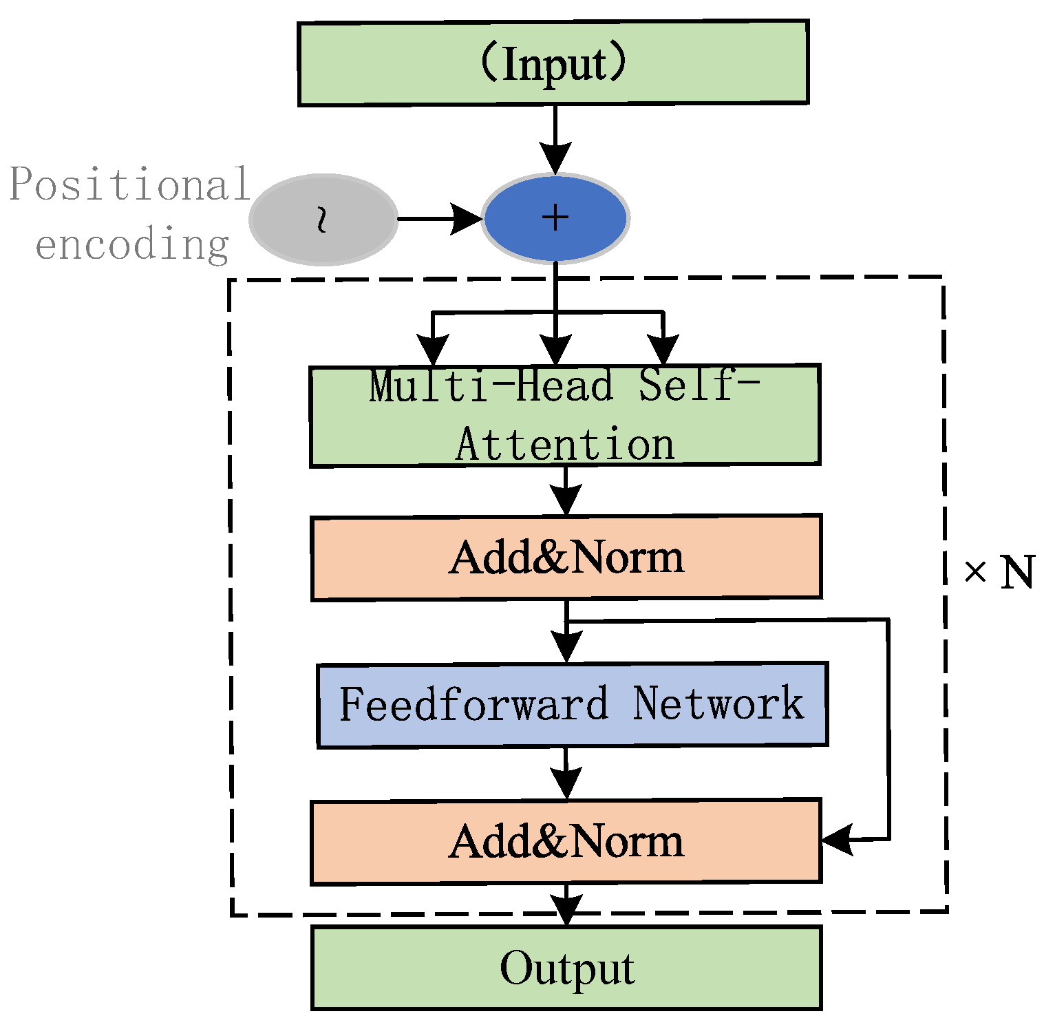
The high-dimensional features obtained by multi-level feature extraction will be input into the fully connected layer to complete further feature compression and classification, and then achieve efficient feature discrimination. This study additionally introduces a federated learning framework to train the FL-RBTNet model, which can not only carry out distributed training under the premise of ensuring data privacy and security, but also make full use of multi-source heterogeneous data, improve the generalization ability and environmental adaptability of the model. It should be emphasized that the federated learning process only transmits model parameters rather than raw data, which significantly reduces the communication overhead and the load of the central server, it is especially suitable for data-sensitive and resource-constrained industrial internet scenarios, which can help to achieve efficient and collaborative intelligent security analysis.
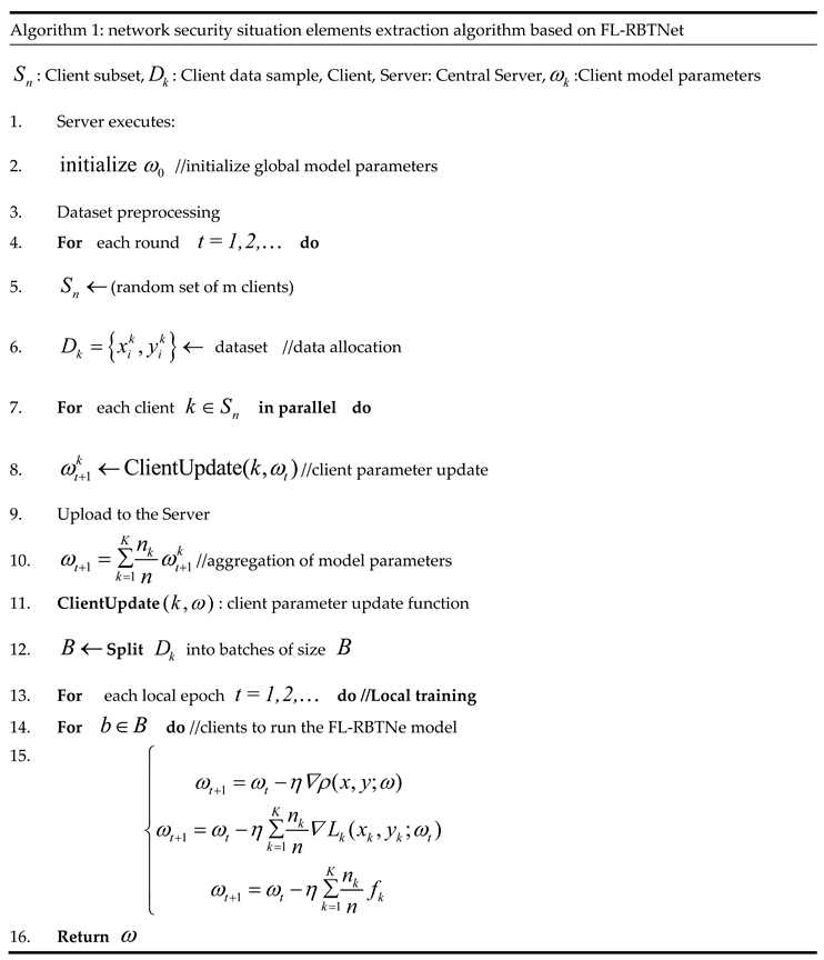
In order to more clearly explain the specific execution steps of the FL-RBTNet model in the process of extracting network security situation elements, the pseudo code description of its core algorithm flow is given, as shown in Algorithm 1. The algorithm shows in detail the operation process of local feature extraction, global parameter aggregation and FL-RBTNe model collaborative modeling under the framework of Federated Learning, it provides a theoretical basis and reference standard for the subsequent system implementation and reproduction.
4. Experiment and Result Analysis
The experiments in this chapter are carried out on a computer configured with 8 GB RAM and Intel (R) Core (TM) i5-8250U CPU@1.60 ghz, running Windows 10, programmed with Python 3.12.0, and using pytorch 1.1.0 + GPU platform to build the model framework. The process of the experiment is as follows.
(1) model initialization: firstly, the goal and Evaluation Index of Federated Learning are determined, and the global model parameters are initialized. At the same time, hyperparameters such as learning rate and batch size are set, and the number of training rounds and stopping conditions of federated learning are clarified. Before starting the training, the data needs to be preprocessed, including feature label separation, numerical coding and format conversion.
(2) client selection and data allocation: a number of clients are randomly selected from the parties participating in federated learning for model training. In order to realize the distributed processing of data, the index mechanism based on client ID is used to randomly distribute the data. Each client is assigned a unique ID, and the data set is divided into subsets based on these ids, which are then randomly assigned to each client for local data processing.
(3) client-side local model training: the Central Server sends the aggregated global model parameters to each client. The client is trained on the local data based on these parameters, and the training process consists of 5 rounds. In each round, the client calculates the loss and gradient, performs forward propagation and back propagation, and continuously optimizes the model.
(4) parameter aggregation: the client uploads the model parameters, loss values and gradient information obtained from local training to the central server. The server integrates the parameters from different clients through an average aggregation strategy, which updates the global model by calculating the average of the model parameters uploaded by all clients.
(5) repeat training and convergence: steps (3) and (4) are repeated until the set stop condition is reached. After each round of training, the server evaluates the performance of the global model, and calculates the accuracy, loss and other indicators on the test set to monitor the change of model performance in real time.
(6) global model evaluation: when the training reaches the stopping condition, the server will evaluate the final global model and calculate its performance index on the independent test set to ensure the validity and robustness of the model.
4.1. Model Performance Evaluation Metrics
In the deep learning model performance evaluation experiment, there are multiple evaluation indexes to comprehensively measure the model performance. Common metrics include ACC, Recall, Precision, and F1-score. The metrics are calculated as follows:
Among them, the true class and the true negative class represent the number of samples correctly classified as attack class and non-attack class respectively, and the false positive class and false negative class represent the number of samples wrongly classified as attack class and non-attack class. ACC represents the proportion of the number of samples correctly predicted by the model to the total number of samples, and Recall represents the proportion of the number of samples correctly predicted by the model to the number of actual positive samples Precision represents the ratio of the number of samples correctly predicted by the model to the number of samples predicted to be positive; F1-score is the harmonic mean of recall and Precision, which is used to comprehensively measure the performance of the model.
4.2. Datasets
Three data sets are used in this experiment. KDD Cup99 is a classic intrusion detection dataset with good uniformity and wide application basis; SCADA2014 is derived from real industrial environments and covers a variety of industrial attack types; Ton-iot2021 integrates multiple data sources of the entire industrial Internet of things system, and is widely used in the training and evaluation of industrial internet intrusion detection models. The above three datasets provide a variety of network security scenarios and attack types for the experiments in this chapter, which helps to verify the generalization ability and overall performance of the model in a distributed environment. Experiments were conducted on the three datasets using five-class, eight-class, and nine-class classifications, respectively.
In order to simulate a more realistic and highly non-independent and identically distributed (non-IID) data silo scenario as much as possible, before the start of federated learning, unlabeled samples were randomly grouped: they were divided into subsets equal to the number of federated learning clients, and these data subsets were then assigned to each client. Each FL client must independently complete data preprocessing before conducting local model training. The data preprocessing methods in this study are the same as those in Chapter 3, including feature-label separation, numerical encoding, and data format conversion. The sample distribution of the FL-RBTNet model is shown in Figure 4. The FL-RBTNet model is trained only locally, with no privacy data exchanged between clients or between clients and the server. This setup aims to maximally reproduce a data silo environment, providing a more realistic testing foundation for subsequent research on distributed training and privacy protection.
4.3. Experimental Parameters
The selection of hyperparameters has an important influence on the performance and generalization ability of the model. Reasonable selection of hyperparameters can not only improve the performance of the model, but also accelerate its convergence speed. In this chapter, the grid search method is used to optimize the hyperparameters, and the specific settings are as follows: the number of clients is 10, the number of client training rounds is 5, and the total training round of federated learning is 10. The weight decay regularization coefficient is set to 0.001, the optimizer uses Adam, and the learning rate is set to 0.005. In addition, the Dropout function is set to a ratio of 0.5, and the batch size is set to 128.

Table 1.
parameter details.
| Parameters | Search area | Optimal value |
| Number of federated learning clients | [5,10,15,20] | 10 |
| Federated learning client model training rounds | [1,3,5,7,9] | 5 |
| Number of federal trainings | [5,10,15,20] | 10 |
| Weight decay | [0.0005,0.001,0.01] | 0.001 |
| Learning rate | [0.0005,0.001,0.005,0.01] | 0.005 |
| Dropout rate | [0.2,0.3,0.4,0.5] | 0.5 |
| Batch size | 32,64,128,256] | 128 |
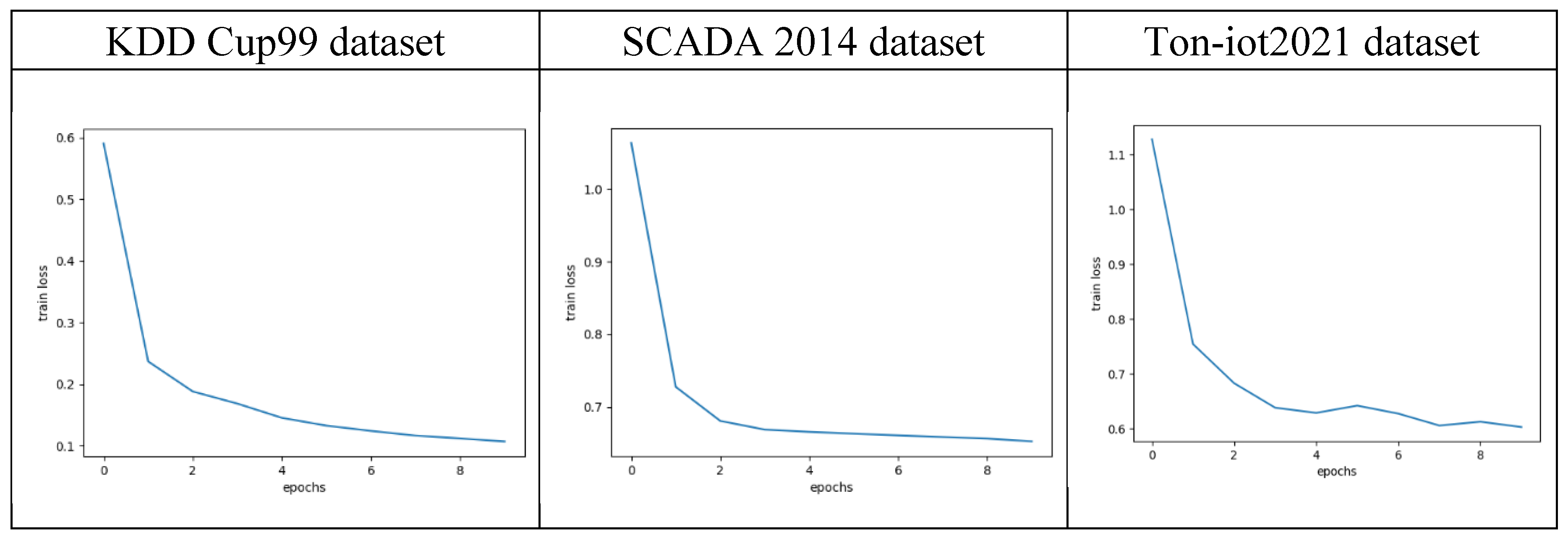
Figure 5 shows the changes in the loss values of the FL-RBTNet model during federated learning. The horizontal axis shows the epochs of federated learning, the vertical axis is the average of the loss values for each of the ten clients in each round of training. From the graph, it can be seen that with the increase of training rounds, the overall loss of the model on the three datasets gradually decreases, indicating that under the synergistic effect of local training and global aggregation of each client, the model performance continues to improve, and the performance of the model is improved, and the convergence effect is better. It is important to note that on the ToN-IoT2021 dataset, there is a brief increase in the loss value at the fifth epoch. This phenomenon is more common in deep learning and federated learning tasks, and may be related to factors such as learning rate settings and heterogeneity of client data distribution. Although there are local fluctuations in the training process, the overall trend is still declining, indicating that the model training process is stable and the optimization effect is good.
4.4. Selection of Model Parameter
In order to further optimize the structural design of the FL-RBTNet model and improve its performance in the task of network security situation element extraction, a series of model parameter selection experiments are carried out in this section, and the results show that the FL-RBTNet model can be used to extract network security situation elements, it aims to evaluate the influence of different key parameter settings on model performance. Specifically, this section explores the influence of the number of convolution layers inside the residual block, the number of residual blocks, the number of BILSTM hidden cells, and the number of Transformer encoder multi-head attention heads on the model performance.
(1) The number of convolution layers inside the residual block
The number of convolution layers inside the residual block directly affects the feature extraction ability and overall complexity of the model. The influence of different settings of convolution layers on the effect of the model is evaluated by experiments, and the results are shown in Tables 2,3 and Table 4. The experimental results show that when the number of convolution layers within the residual block is 2, the ACC of the model on the KDD Cup, SCADA2014, and ToN-IoT2021 datasets is 98.89% , 98.91% , and 98.12% , respectively, which are better than the 1-layer and 3-layer structures. The results show that the number of convolution layers has a significant impact on the feature extraction ability. If the number of convolution layers is too small, the model can not effectively capture the complex local features in the data; while too many convolution layers, although it can enhance the ability of feature modeling, it also increases the computational complexity, and it can improve the accuracy of feature modeling, it is easy to lead to gradient disappearance or overfitting, especially when the data sample is limited or the distribution is complex. This is further validated by a 3.8% reduction in ACC at 3 layers of convolution compared to 2 layers for this high-dimensional heterogeneous dataset, ToN-IoT2021.
Table 2.
the effect of the number of convolutional layers within the residual block on the model-KDD Cup99 dataset (%).
Table 2.
the effect of the number of convolutional layers within the residual block on the model-KDD Cup99 dataset (%).
| Number of convolutional layers | ACC | Recall | Precision | F1-score |
| 1 | 98.50 | 98.47 | 98.55 | 98.51 |
| 2 | 98.89 | 98.87 | 98.93 | 98.90 |
| 3 | 97.66 | 97.57 | 97.67 | 97.62 |
Table 3.
the effect of the number of convolutional layers within the residual block on the model-SCADA2014 dataset (%).
Table 3.
the effect of the number of convolutional layers within the residual block on the model-SCADA2014 dataset (%).
| Number of convolutional layers | ACC | Recall | Precision | F1-score |
| 1 | 98.12 | 97.79 | 98.15 | 97.97 |
| 2 | 98.91 | 98.85 | 98.99 | 98.92 |
| 3 | 97.55 | 97.22 | 97.62 | 97.42 |
Table 4.
the effect of the number of convolutional layers within the residual block on the model-ToN-IoT2021 dataset (%).
Table 4.
the effect of the number of convolutional layers within the residual block on the model-ToN-IoT2021 dataset (%).
| Number of convolutional layers | ACC | Recall | Precision | F1-score |
| 1 | 97.57 | 97.05 | 97.25 | 97.02 |
| 2 | 98.12 | 97.52 | 99.09 | 97.43 |
| 3 | 94.32 | 89.55 | 93.18 | 91.04 |
(2) Number of residual blocks
The number of residual blocks affects the depth and complexity of feature extraction in the local spatial dimension. By setting different numbers of residual blocks (2,4,6) , the experimental results are shown in Tables 5,6, and 7. The results show that the performance of the model is the best when there are four residual blocks. On the KDD Cup dataset, the ACC of the 4 residual blocks is 1.71% and 1.91% higher than that of the 2 and 6 residual blocks, respectively; on the SCADA2014 dataset, the ACC of the 4 residual blocks is 0.98% and 1.45% higher than that of the 2 and 6 residual blocks, respectively; On the ToN-IoT2021 dataset, the ACC of the 4 residual blocks was 0.88% and 2.39% higher than those of 2 and 6, respectively. These results show that too few residual blocks can cause the model to fail to capture complex local spatial features, while too many residual blocks may increase computational complexity, introduce redundant features and lead to overfitting. Therefore, an appropriate number of residual blocks can effectively balance the feature extraction ability and computational efficiency, thereby improving the model performance.
Table 5.
the effect of the number of residual blocks on model performance-KDD CUP99 dataset (%).
| Number of residual blocks N | ACC | Recall | Precision | F1-score |
| 2 | 97.18 | 96.65 | 97.11 | 96.88 |
| 4 | 98.89 | 98.87 | 98.93 | 98.90 |
| 6 | 96.98 | 96.47 | 96.89 | 96.68 |
Table 6.
effect of number of residual blocks on model performance-SCADA2014 dataset (%).
| Number of residual blocks N | ACC | Recall | Precision | F1-score |
| 2 | 97.93 | 97.61 | 97.99 | 97.80 |
| 4 | 98.91 | 98.85 | 98.99 | 98.92 |
| 6 | 97.46 | 97.13 | 97.53 | 97.33 |
Table 7.
effect of number of residual blocks on model performance-ToN-IoT2021 dataset (%).
| Number of residual blocks N | ACC | Recall | Precision | F1-score |
| 2 | 97.24 | 96.07 | 97.33 | 96.57 |
| 4 | 98.12 | 97.52 | 99.09 | 97.43 |
| 6 | 95.73 | 95.14 | 92.39 | 93.24 |
Table 8.
effect of the number of BILSTM hidden units on the model-KDD Cup99 dataset (%).
| BILSTM hides the number of cells | ACC | Recall | Precision | F1-score |
| 64 | 97.98 | 97.89 | 97.97 | 97.93 |
| 128 | 98.89 | 98.87 | 98.93 | 98.90 |
| 256 | 97.38 | 97.13 | 97.29 | 97.21 |
Table 9.
BILSTM effect of hidden cell number on model-SCADA2014 dataset (%).
| BILSTM hides the number of cells | ACC | Recall | Precision | F1-score |
| 64 | 98.40 | 98.08 | 98.46 | 98.27 |
| 128 | 98.91 | 98.85 | 98.99 | 98.92 |
| 256 | 97.69 | 97.37 | 97.79 | 97.58 |
Table 10.
effect of number of hidden cells in BiLSTM-ToN-IoT2021 dataset (%).
| BILSTM hides the number of cells | ACC | Recall | Precision | F1-score |
| 32 | 98.00 | 95.72 | 95.91 | 95.50 |
| 64 | 98.12 | 97.52 | 99.09 | 97.43 |
| 128 | 96.88 | 94.99 | 95.77 | 95.11 |
(4) Transformer encoder multi-head attention head count
The multi-head attention mechanism in Transformer encoder can capture the global dependencies between input features in parallel. The experimental results are shown in Tables 11,12, and 13. The results show that the model performs best when the number of heads with multi-head attention is 6, and ACC on the three datasets performs better than 4 and 8 heads, respectively, other metrics such as recall, precision, and F1-score also achieved the best results. When the number of headers is small, it may be difficult to cover all important feature relationships, resulting in insufficient understanding of the global context of the model; when the number of headers is too large, the subspace dimension that each attention head can express is reduced, and the number of headers is too large, may lead to a decline in model performance, while increasing computational resource consumption and overfitting risk.
Table 11.
effects of the number of headers of encoder multi-headers' attention on model performance-KDD CUP99 dataset (%).
Table 11.
effects of the number of headers of encoder multi-headers' attention on model performance-KDD CUP99 dataset (%).
| Attention head count | ACC | Recall | Precision | F1-score |
| 4 | 96.58 | 96.64 | 96.66 | 96.60 |
| 6 | 98.89 | 98.87 | 98.93 | 98.90 |
| 8 | 95.97 | 95.25 | 96.54 | 95.89 |
Table 12.
effect of the number of headers of encoder multi-head attention on model performance-SCADA2014 dataset (%).
Table 12.
effect of the number of headers of encoder multi-head attention on model performance-SCADA2014 dataset (%).
| Attention head count | ACC | Recall | Precision | F1-score |
| 4 | 97.45 | 97.08 | 97.41 | 97.25 |
| 6 | 98.91 | 98.85 | 98.99 | 98.92 |
| 8 | 96.33 | 96.00 | 96.16 | 96.08 |
Table 13.
effect of the number of headers of encoder multi-head attention on model performance-ToN-IoT2021 dataset (%).
Table 13.
effect of the number of headers of encoder multi-head attention on model performance-ToN-IoT2021 dataset (%).
| Attention head count | ACC | Recall | Precision | F1-score |
| 4 | 97.68 | 97.07 | 97.40 | 97.12 |
| 6 | 98.12 | 97.52 | 99.09 | 97.43 |
| 8 | 97.46 | 96.57 | 97.36 | 96.84 |
4.5. Ablation Test
Ablation experiments are a standard way to assess the importance of the various components in a model. By removing or replacing specific modules in turn and observing the subsequent changes in model performance, the contribution of each component to the overall system performance can be analyzed quantitatively and qualitatively. To gain insight into the effectiveness and relative importance of each core module in the FL-RBTNet model, a series of ablation experiments were conducted in this section. The FL-RBTNet model is mainly composed of three key functional modules: ResNet, BILSTM, and Transformer. Accordingly, six experimental configurations are designed to investigate the performance changes, and the performance of the fl-rbtnet model is analyzed, they are: Resnet only, BILSTM only, ResNet-transformer hybrid model, BiLSTM-transformer hybrid model, ResNet-BiLSTM hybrid model, and the complete FL-RBTNet (which integrates all three modules) . The ablation experimental results on the three datasets are shown in Figures 6,7, and 8, respectively.
Figure 6.
Ablation experiments on KDD Cup99 dataset
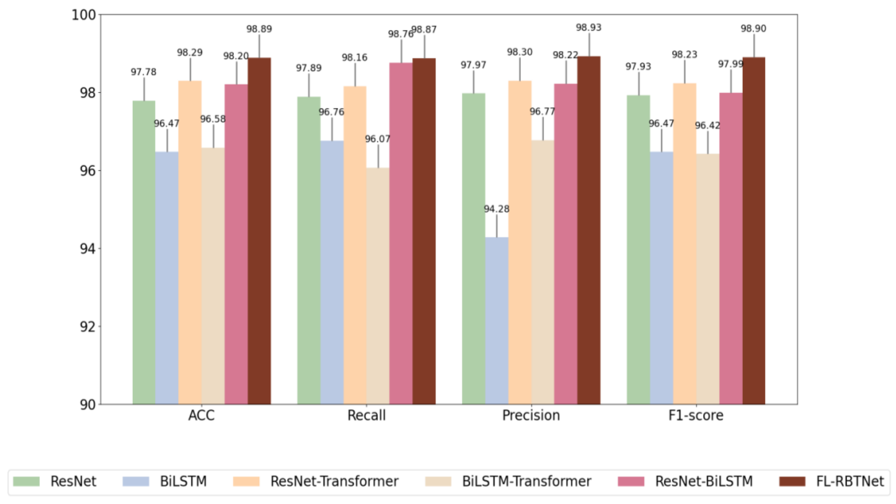
Figure 7.
Ablation experiments on the SCADA2014 dataset
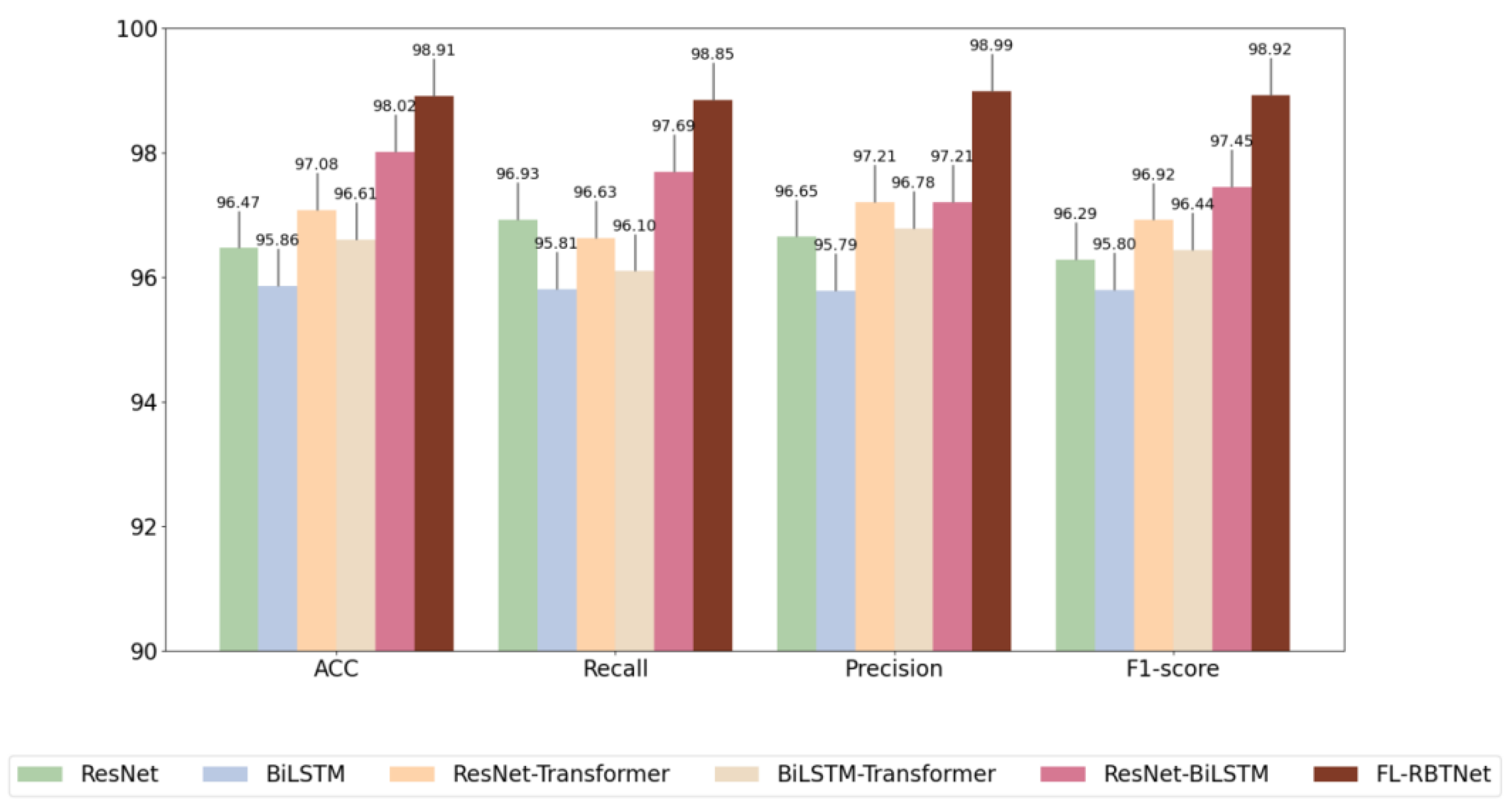
Figure 8.
Ablation experiments on the ToN-IoT2021 dataset
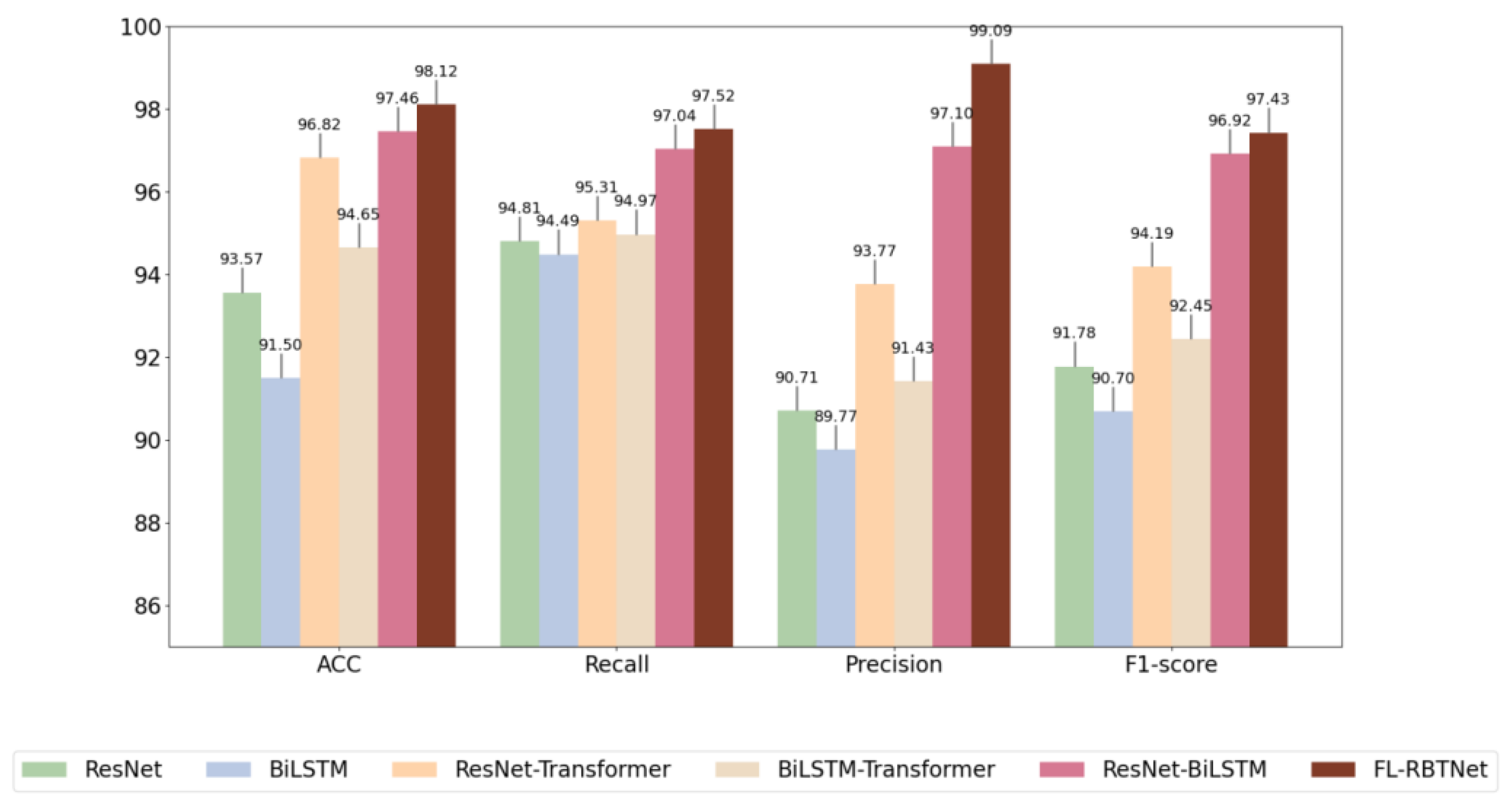
Observing the three graphs, it can be seen that Resnet alone and BILSTM alone perform poorly, which may be due to the fact that this may be due to their ability to extract features only from a single dimension of the spatial local or temporal series, respectively, and the fact that Resnet alone and BILSTM alone perform poorly, lack of collaborative modeling ability for multi-dimensional information in complex network traffic data. The performance of the combined ResNet-BiLSTM module on the three datasets has been significantly improved, which is due to the ability of the structure to simultaneously extract spatial local features and temporal dependence information in network traffic, and to improve the performance of the combined ResNet-BiLSTM module, thus, the recognition ability of the model for complex attack behaviors is improved. Resnet and BILSTM alone also show performance improvements with the addition of the Transformer module because of Transformer's powerful global modeling capabilities, it can capture the long-distance dependencies and global context information between features through the multi-head self-attention mechanism. FL-RBTNet achieved relatively better results on multiple evaluation indicators, reaching 98.89% ACC on the KDD Cup99 dataset, 98.91% ACC on the SCADA2014 dataset, and 98.12% ACC on the ToN-IoT2021 dataset. This result reflects the complementary advantages of ResNet, BiLSTM and Transformer in local feature extraction, temporal dependence modeling and global feature modeling, it can help the model to deeply characterize complex network traffic data from multiple dimensions, thus showing good performance in the situation element extraction task under the Federated Learning Architecture.
4.6. Comparative Experiments
To comprehensively evaluate the effectiveness and advantages of the proposed FL-RBTNet model, this section conducts comparative experiments with other models and different structural combinations on an independent test set. Specifically, FL-RBTNet was compared with PNN, KNN, RF, Transformer, cgan-Transformer on KDD Cup99 dataset; FL-RBTNet was compared with CNN-GRU, RNN, LSTM, Transformer, Res-CNN-SRU on SCADA2014 dataset; FL-RBTNet was compared with CNN-GRU, RNN, LSTM, Transformer, Res-CNN-SRU on ToN-IoT2021 dataset; FL-RBTNet was compared with PNN, KNN, RF, Transformer, cgan-Transformer on KDD Cup99 dataset; FL-RBTNet was compared with CNN-GRU, RNN, LSTM, Transformer, RES - FL-RBTNet is compared with PNN, KNN, RF, Deepak-iot, E-ADS, and SATIDS, which is an intrusion detection system based on improved LSTM. The experimental results are shown in Table 14 and Table 15, and 16.
Table 14.
comparison of classification effects of different situation elements extraction models-KDD Cup99 dataset (%).
Table 14.
comparison of classification effects of different situation elements extraction models-KDD Cup99 dataset (%).
| Models | ACC | Recall | Precision | F1-Score |
| PNN | 90.76 | 90.75 | 98.18 | 94.32 |
| Knn | 90.19 | 90.18 | 98.20 | 94.02 |
| Speaking | 87.95 | 87.94 | 89.03 | 88.48 |
| Transformer | 91.01 | 91.01 | 91.85 | 91.43 |
| CGAN-transformer | 93.07 | 93.07 | 94.29 | 93.68 |
| FL-RBTNet | 98.89 | 98.87 | 98.93 | 98.90 |
Table 15.
comparison of classification effects of different situation element extraction models-SCADA2014 dataset (%).
Table 15.
comparison of classification effects of different situation element extraction models-SCADA2014 dataset (%).
| Models | ACC | Recall | Precision | F1-score |
| CNN-GRU | 94.69 | 78.92 | 78.94 | 75.45 |
| RNN | 94.95 | 78.17 | 78.89 | 77.98 |
| LSTM | 95.25 | 95.25 | 95.49 | 95.30 |
| Transformer | 95.07 | 95.07 | 91.85 | 93.43 |
| Res-cnn-sru | 98.79 | 95.04 | 95.34 | 95.38 |
| FL-RBTNet | 98.91 | 98.85 | 98.99 | 98.92 |
Table 16.
comparison of classification effects of different situation elements extraction models-ToN-IoT2021 dataset (%).
Table 16.
comparison of classification effects of different situation elements extraction models-ToN-IoT2021 dataset (%).
| Models | ACC | Recall | Precision | F1-Score |
| PNN | 88.15 | 79.84 | 85.80 | 82.71 |
| Knn | 89.91 | 89.93 | 89.81 | 88.38 |
| Speaking | 93.94 | 92.38 | 86.87 | 91.81 |
| Deepak-iot | 90.57 | 88.23 | 89.59 | 88.87 |
| E-ADS | 96.35 | / | 90.55 | 95.03 |
| Satids | 96.56 | 97.40 | 97.30 | 97.35 |
| FL-RBTNet | 98.12 | 97.52 | 99.09 | 97.43 |
Observing the three tables, it can be seen that the FL-RBTNet model shows better performance on four key indicators on the three datasets, especially on Recall, Precision, and F1-Score indicators, compared with the comparison model, and the FL-RBTNet model shows better performance on Recall, Precision, and F1-Score, compared with the comparison model. This shows that FL-RBTNet has strong robustness and accuracy when dealing with data sets of different types and sizes. The ACC, Recall, Precision, and F1-score of FL-RBTNet on the KDD Cup99 dataset are 98.89% , 98.87% , 98.93% , and 98.90% , respectively; The ACC, Recall, Precision, and F1-score of FL-RBTNet on the SCADA2014 dataset were 98.91% , 98.85% , 98.99% , and 98.92% , respectively; The ACC, Recall, Precision, and F1-score of FL-RBTNet on the ToN-IoT2021 dataset were 98.12% , 97.52% , 99.09% , and 97.43% , respectively. The ResNet module can effectively extract the local structural features of the network traffic data, which is mainly due to its powerful feature extraction and modeling capabilities The BILSTM module is modeled from the forward and backward time dimensions, which can capture the context dependencies in time series data more fully The multi-head self-attention mechanism in the Transformer module gives the model the ability to model global dependencies, and enhances the model's ability to focus on important features. In addition, with the support of the Federated Learning Framework, the FL-RBTNet model can integrate multi-source data knowledge in a distributed environment to achieve the unity of privacy protection and performance improvement. This privacy protection capability is particularly important for dealing with sensitive data, which makes the FL-RBTNet model have obvious advantages in application scenarios that require strict data protection.
5. Conclusion
Aiming at the problem of insufficient data privacy protection and sharing in the extraction of industrial internet security situation elements, this paper proposes a FL-RBTNet model that integrates federated learning and deep learning. The model integrates ResNet, BILSTM and Transformer architectures to enhance the ability of multi-dimensional feature extraction. The distributed training is realized through the Federated Learning Framework, which protects data privacy and alleviates the problem of data islands. Experiments show that flrbtnet is superior to the comparison method in key indicators such as precision and recall rate, which effectively improves the extraction effect of situation elements and provides a feasible scheme for industrial internet security awareness.
Author Contributions
All authors contributed equally to this work. All authors have read and agreed to the published version of the manuscript.
Funding
This work was supported in part by Henan Province Science and Technology Research Project (No.252102210183), Zhengzhou Collaborative Innovation Project (No. 2021ZDPY0106) and horizontal project (No. JSJ202503011).
Data Availability Statement
The data that supports the research findings provided in the article.
Acknowledgments
We would like to thank all the reviewers for their valuable comments.
Conflicts of Interest
The authors declare no conflict of interest.
References
- Hu, K.; Gong, s.; Zhang, Q.; et al. An overview of implementing security and privacy in federated learning. ARTIF Intell Rev 2024, 57, 204. [Google Scholar] [CrossRef]
- Laine, R; Chughtai, B; Betley, J; et al. Me, myself, and Ai: The Situational Awareness Dataset (sad) for LLMS. Advances in Neural Information Processing Systems 2024, 37, 64010–64118. [Google Scholar]
- Xu, C; Wu, J; Zhang, F; et al. A deep image classification model based on prior feature knowledge embedding and application in medical diagnosis. Scientific Reports 2024, 14(1), 13244. [Google Scholar] [CrossRef]
- Sikiru, i. A.; Kora, A. D.; Ezin, E. C...; et al. Hybridization of Learning Techniques and Quantum Mechanism for IIOT Security: Applications, Challenges, and pospects. Electronics 2024, 13, 4153. [Google Scholar] [CrossRef]
- D'Agostino, P.; Violante, M.; Macario, G. a Scalable Fog Computing Solution for Industrial Predictive Maintenance and Customization. Electronics 2025, 14, 24. [Google Scholar] [CrossRef]
- Rafique, W. W.; Qadir, J. Internet of everything meets the Metaverse: Bridging physical and virtual worlds with blockchain. Computer Science Review 2024, Vol. 54, 100678. [Google Scholar] [CrossRef]
- Rjoub, G.; Wahab, O. A.; Bentahar, J.; et al. Trust-driven reinforcement selection strategy for federated learning on IoT devices. Computing 2024, 106, 1273–1295. [Google Scholar] [CrossRef]
- Wang Jun, Wang Hualin, Huang Bowen, et al. Industrial IoT Intrusion Detection Based on Federated Learning and self-attention. Journal of Jilin University (Engineering Edition) 2023, 53(11), 3229–3237.
- Anton, S. D. D.; Sinha, S.; Schotten, H. D. Anomaly Detection in IIoT: A Systematic Literature Review. IEEE Access 2023, vol. 11, 3672–3693. [Google Scholar]
- Qi, L.; Hu, Y.; Zhang, X.; et al. Privacy-Aware Data Fusion and Prediction with Spatial-Temporal Context for Smart City Industrial Environment. IEEE Transactions on Industrial Informatics 2023, vol. 19(no. 5), 6960–6970. [Google Scholar] [CrossRef]
- Zhang, J.; Pan, L.; Han, Q.; et al. "Deep Learning Based Attack Detection for Industrial Control System: A Survey. IEEE/CAA Journal of Automatica Sinica 2022, vol. 9(no. 10), 1751–1776. [Google Scholar] [CrossRef]
- H. Li, P. Oulaïdah, N. S. Rosenbloom, et al., "Deep Learning-based Anomaly Detection in Industrial Control Systems: A Survey," in IEEE Communications Surveys & Tutorials, vol. 24, no. 4, pp. 2441-2469, 2022.Xie Chengzong, Wang Yuhe, Wang Baiduo, et al. . An Industrial Internet of Things Intrusion Detection Method Based on gru-fedadam. Cyber Security & Data Governance, 2024,43(2) : 9-15.
- Liang, W.; Luo, Y.; Zhao, L.; Wu, Y. Deep Learning-Based Network Intrusion Detection for Industrial Internet of Things. IEEE Transactions on Industrial Informatics 2023, vol. 19(no. 3), 2450–2459. [Google Scholar]
- Saba, T.; Rehman, A.; Sadad, T.; et al. "CNN- and RNN-Based Hybrid Approach to Detect Malicious Traffic in IoT Networks. IEEE Transactions on Industrial Informatics 2022, vol. 18(no. 12), 8769–8778. [Google Scholar]
- Yang, L.; Moubayed, A.; Shami, A. MTH-IDS: A Multitiered Hybrid Intrusion Detection System for Internet of Vehicles. IEEE Internet of Things Journal 2022, vol. 9(no. 1), 616–632. [Google Scholar] [CrossRef]
- Liu, G.; Zhang, J.; Wang, W.; et al. "A Transformer-Based Intrusion Detection System for IoT Networks. IEEE Internet of Things Journal 2023, vol. 10(no. 13), 11526–11536. [Google Scholar]
- Nguyen, D. C.; Ding, M.; Pathirana, P. N.; et al. Federated Learning for Internet of Things: A Comprehensive Survey. IEEE Communications Surveys & Tutorials 2022, vol. 24(no. 3), 1622–1658. [Google Scholar]
- Hu, K.; Gong, s.; Zhang, Q.; et al. Security and Privacy Issues in Industrial Internet of Things: A Federated Learning Approach. International Journal of Industrial Internet of Things 2024. [Google Scholar]
- He, F; Liu, T; Tao, D. Why resnet works? Residuals generalize [ j ]. IEEE Transactions on Neural Networks and learning systems 2020, 31(12), 5349–5362. [Google Scholar] [CrossRef] [PubMed]
- Ye, P; He, t; Tang, S; et al. Stimulative training + +: Go beyond the performance limits of residual networks [ J ]. IEEE Transactions on Pattern Analysis and Machine Intelligence 2025, 1–17. [Google Scholar] [CrossRef] [PubMed]
- Alizadegan, H; Rashidi Malki, B; Radmehr, A; et al. Comparative study of long short-term memory (LSTM), bidirectional LSTM, and traditional machine learning approaches for energy consumption prediction [ J ]. Energy Exploration & Exploitation 2025, 43(1), 281–301. [Google Scholar]
- Liu, y; Li, D; Wan, s; et al. A long short-term memory-based model for greenhouse climate prediction [ j ]. International Journal of Intelligent Systems 2022, 37(1), 135–151. [Google Scholar] [CrossRef]
- Zhang, w t; Bai, y; Zheng, S D; et al. Tensor Transformer for hyperspectral image classification [ J ]. Pattern Recognition 2025, 163, 111470. [Google Scholar] [CrossRef]
Figure 1.
FL-RBTNet structure diagram.
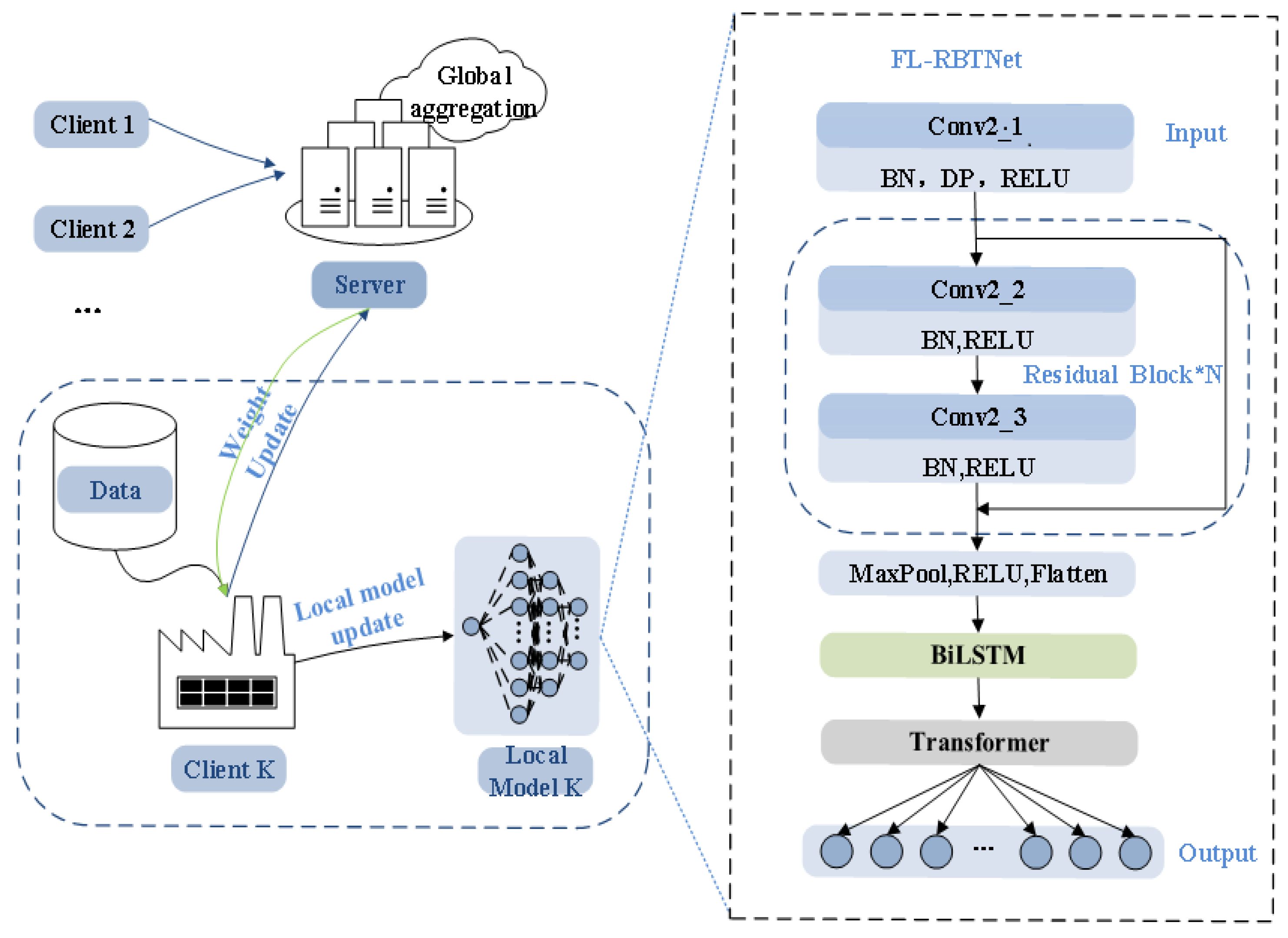
Figure 2.
residual network structure
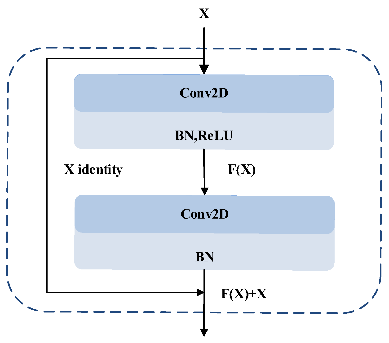
Figure 4.
Data silo scenario sample distribution
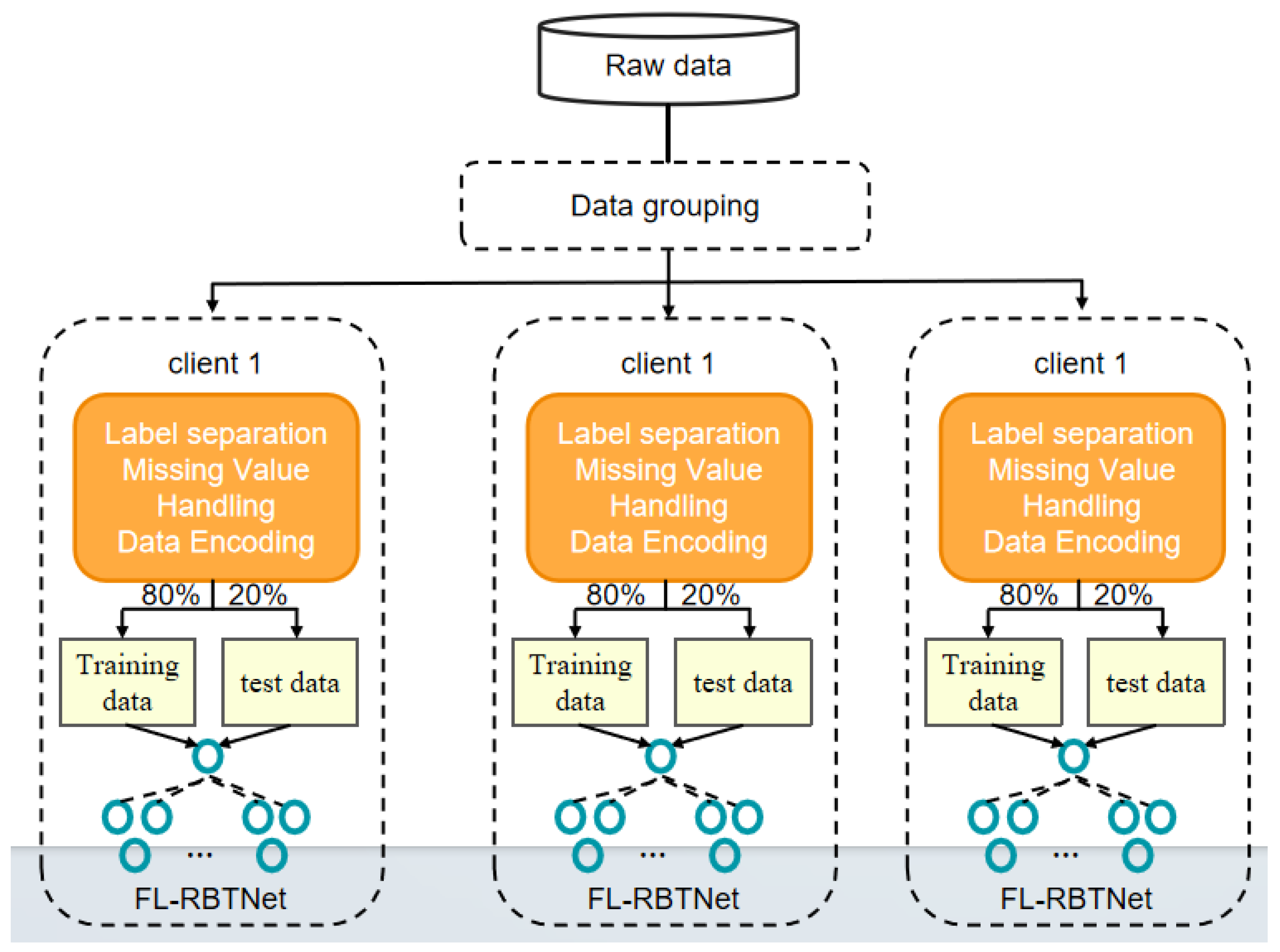
Figure 5.
changes of loss values on different data sets.
Disclaimer/Publisher’s Note: The statements, opinions and data contained in all publications are solely those of the individual author(s) and contributor(s) and not of MDPI and/or the editor(s). MDPI and/or the editor(s) disclaim responsibility for any injury to people or property resulting from any ideas, methods, instructions or products referred to in the content. |
© 2026 by the authors. Licensee MDPI, Basel, Switzerland. This article is an open access article distributed under the terms and conditions of the Creative Commons Attribution (CC BY) license (http://creativecommons.org/licenses/by/4.0/).
Copyright: This open access article is published under a Creative Commons CC BY 4.0 license, which permit the free download, distribution, and reuse, provided that the author and preprint are cited in any reuse.


