A Truncated Quasiconformal Energy for the Riemann ξ-Function and Sharp Extremal–Length/Teichmüller Lower Bounds

1. Introduction

Let $\xi \left(s\right):=\frac{1}{2}s(s-1){\pi }^{-s/2}\Gamma \left({\displaystyle \frac{s}{2}}\right)\zeta \left(s\right)uad(s\in \mathbb{C})$ be the completed Riemann $\xi$–function. It is entire of order 1, satisfies $\xi \left(\overline{s}\right)=\overline{\xi \left(s\right)},uad\xi (1-s)=\xi \left(s\right),$ and its zeros in the critical strip $\Sigma :=\{s\in \mathbb{C}:0<Res<1\}$ are exactly the nontrivial zeros of $\zeta$.

This note formalizes a single geometric idea:

An “infinite-energy obstruction” typically arises as a limit $T\to \infty$ of a family of finite-window problems. The same unbounded energy is therefore simultaneously an obstruction to a global bounded-distortion scenario and the generator of an infinite hierarchy of finite-stage quantitative questions.

Concretely, we define for each height cutoff $T>0$ an energy $E_{\xi }\left(T\right)$ as an infimum of $logK$ over a class of quasiconformal maps satisfying a corridor control constraint. We then derive sharp extremal-length lower bounds for $E_{\xi }\left(T\right)$ and for the associated Teichmüller-type energy $d_{\xi }\left(T\right)={\displaystyle \frac{1}{2}}{E}_{\xi }\left(T\right)$.

Remark 1

(Scope and honesty). Nothing in this paper proves RH or rules out off-critical zeros unconditionally. The functional $E_{\xi }\left(T\right)$ is a geometric energy attached to a specific deformation problem (corridor-controlled axis landing on a finite window). It is meaningful whether or not RH is true, because it is defined by an infimum (which may be $+\infty$ if the admissible class is empty).

2. Windowed Representative Off-Critical Zeros and a Canonical Corridor Radius

Let $Z:=\{\rho \in \Sigma :\xi (\rho )=0\}$ denote the set of nontrivial zeros in the strip, counted without multiplicity (for our geometric constructions, coincident zeros are a single puncture).

We will work with a uniform decomposition of the height axis into disjoint “levels” of equal height, with a buffer region that enforces disjointness.

2.1. Level intervals

Fix once and for all the level half-height $H_0:=1.$ For each $j\in \mathbb{Z}$ define the full level interval and its core by

$$I_j:=\left(2j-H_0,2j+H_0\right)=(2j-1,2j+1),uad{I}_j^{\mathrm{core}}:=\left(2j-\frac{1}{2},2j+\frac{1}{2}\right).$$

(1)

Then:

• the full intervals $I_j$ are pairwise disjoint (as open sets) and tile $\mathbb{R}$ up to endpoints;
• the core intervals $I_j^{\mathrm{core}}$ are pairwise disjoint and satisfy $(I_j^{\mathrm{core}},I_{j^{\prime }}^{\mathrm{core}})\ge 1uad(j\ne j^{\prime }).$

2.2. Representative Off-Critical Zeros Per Level

We will select at most one representative left-half zero per level, using a deterministic rule.

Definition 1

(Active levels and representative left zero). Let $T>0$. Define the set of indices whose levels lie in the window by $\mathcal{J}\left(T\right):=\{j\in \mathbb{Z}:I_j(-T,T)\}.$ (Equivalently, $\left|2j\right|<T-1$.)

For $j\in \mathcal{J}\left(T\right)$ define the set of left-half zeros in the core by $Z_j\left(T\right):=\{\rho \in Z:Im\rho \in I_j^{\mathrm{core}},Re\rho <\frac{1}{2}\}.$ Call j active if $Z_j\left(T\right)\ne ⌀$, and set ${\mathcal{J}}_{\xi }\left(T\right):=\{j\in \mathcal{J}\left(T\right):Z_j\left(T\right)\ne ⌀\}.$

If $j\in {\mathcal{J}}_{\xi }\left(T\right)$, choose a representative zero ${\rho }_j\left(T\right)\in Z_j\left(T\right)\mathrm{such}\mathrm{that}Re{\rho }_j\left(T\right)={max}_{\rho \in Z_j\left(T\right)}Re\rho ,$ and write ${\rho }_j\left(T\right)=:{\sigma }_j\left(T\right)+\mathrm{i}{t}_j\left(T\right),uad{\delta }_j\left(T\right):=\frac{1}{2}-{\sigma }_j\left(T\right)>0.$

Remark 2.

The rule “choose the left-half zero closest to the critical line within the core” is deterministic (hence canonical in an NT sense) and ensures that, at a fixed level, all other left-half zeros in the core are farther left, hence their discs of a common radius lie outside the corridor we will define.

2.3. Canonical Corridor Radius

We choose a radius that is small enough to ensure: (i) discs sit well inside the strip rectangle, and (ii) discs do not cross the critical line for these left-half representatives.

Definition 2

(Canonical corridor radius). Let $T>0$. If ${\mathcal{J}}_{\xi }\left(T\right)\ne ⌀$, set ${\delta }_{min}\left(T\right):={min}_{j\in {\mathcal{J}}_{\xi }\left(T\right)}{\delta }_j\left(T\right)\in (0,1/2].$ If ${\mathcal{J}}_{\xi }\left(T\right)=⌀$, set ${\delta }_{min}\left(T\right):=\frac{1}{4}$.

Define the corridor radius by

$$r_{\xi }\left(T\right):=min\left\{{\displaystyle \frac{1}{1000}},{\displaystyle \frac{1}{4}},{\displaystyle \frac{{\delta }_{min}\left(T\right)}{4}}\right\}.$$

(2)

Remark 3.

If ${\mathcal{J}}_{\xi }\left(T\right)$ is nonempty, then $r_{\xi }\left(T\right)\le {\delta }_{min}\left(T\right)/4$ ensures that for every active level j, ${\sigma }_j\left(T\right)\le \frac{1}{2}-{\delta }_{min}\left(T\right)\le \frac{1}{2}-4r_{\xi }\left(T\right),$ so the disc $D({\rho }_j\left(T\right),r_{\xi }\left(T\right))$ lies strictly in the left half of the strip.

3. Axis-Landing Source/Target Domains and the Energy $E_{\xi }\left(T\right)$

3.1. The Strip Rectangle Window

For $T>0$ define the window rectangle $R_T:=\{x+\mathrm{i}y\in \mathbb{C}:0<x<1,|y|<T\}.$

3.2. Source and Target Puncture Sets

Fix $T>0$ and write $r:=r_{\xi }\left(T\right)$ for brevity.

Definition 3

(Source punctures from representative off-critical zeros). For each active level $j\in {\mathcal{J}}_{\xi }\left(T\right)$ define the symmetric pair at height $t_j\left(T\right)$: ${\rho }_j:={\rho }_j\left(T\right)={\sigma }_j\left(T\right)+\mathrm{i}{t}_j\left(T\right),uad{\rho }_j^{*}:=1-{\rho }_j=(1-{\sigma }_j\left(T\right))+\mathrm{i}{t}_j\left(T\right).$ Define the source puncture set $P_{\xi }^{\mathrm{src}}\left(T\right):={\bigcup }_{j\in {\mathcal{J}}_{\xi }\left(T\right)}\{{\rho }_j,{\rho }_j^{*}\}.$

Remark 4.

We do not include the full set of zeros of ξ in the window; we include only one canonical off-critical pair per active level. This is deliberate: it produces a disjoint stack of corridors to which extremal length applies cleanly.

Definition 4

(Axis-landing target punctures). Let $r=r_{\xi }\left(T\right)$. Define the fixed (per-T) axis-landing horizontal offset ${\delta }_{\mathrm{ax}}\left(T\right):=2r.$ For each active level $j\in {\mathcal{J}}_{\xi }\left(T\right)$ define the target centers at the same height $t_j\left(T\right)$: ${\rho }_{j,\mathrm{ax}}:=\left(\frac{1}{2}-{\delta }_{\mathrm{ax}}\left(T\right)\right)+\mathrm{i}{t}_j\left(T\right)=\left(\frac{1}{2}-2r\right)+\mathrm{i}{t}_j\left(T\right),uad{\rho }_{j,\mathrm{ax}}^{*}:=\left(\frac{1}{2}+{\delta }_{\mathrm{ax}}\left(T\right)\right)+\mathrm{i}{t}_j\left(T\right)=\left(\frac{1}{2}+2r\right)+\mathrm{i}{t}_j\left(T\right).$ Define the target puncture set $P_{\xi }^{\mathrm{tgt}}\left(T\right):={\bigcup }_{j\in {\mathcal{J}}_{\xi }\left(T\right)}\{{\rho }_{j,\mathrm{ax}},{\rho }_{j,\mathrm{ax}}^{*}\}.$

3.3. The Domains

Definition 5

(Source/target domains). Let $r=r_{\xi }\left(T\right)$. Define the source domain ${\Omega }_{\xi }^{\mathrm{src}}\left(T\right):=R_T\setminus {\bigcup }_{p\in P_{\xi }^{\mathrm{src}}\left(T\right)}D(p,r),$ and the target domain ${\Omega }_{\xi }^{\mathrm{tgt}}\left(T\right):=R_T\setminus {\bigcup }_{p\in P_{\xi }^{\mathrm{tgt}}\left(T\right)}D(p,r).$

Remark 5

(Disjointness is automatic). Because each representative height $t_j\left(T\right)$ lies in the core $I_j^{\mathrm{core}}$ and the cores are separated by at least 1, and because $r\le 1/4$, the discs in distinct levels are disjoint. Horizontally, the left and right discs in the same level are separated by at least $1-2{\sigma }_j\left(T\right)-2r>0$ (see below).

3.4. Corridors and corridor control

For each active level j define the middle corridor strip in that level:

$$Q_j^{\mathrm{src}}\left(T\right):=\left({\sigma }_j\left(T\right)+r,1-{\sigma }_j\left(T\right)-r\right)\times I_j,uad{Q}_j^{\mathrm{tgt}}\left(T\right):=\left(\frac{1}{2}-r,\frac{1}{2}+r\right)\times I_j.$$

(3)

The key geometric fact is that $Q_j^{\mathrm{src}}\left(T\right)$ is disjoint from the two discs around ${\rho }_j$ and ${\rho }_j^{*}$ because the left disc lies in $x\le {\sigma }_j+r$ and the right disc lies in $x\ge 1-{\sigma }_j-r$ for all y.

Define the corridor widths:

$$w_j^{\mathrm{src}}\left(T\right):=\left(1-{\sigma }_j\left(T\right)-r\right)-\left({\sigma }_j\left(T\right)+r\right)=1-2{\sigma }_j\left(T\right)-2r=2{\delta }_j\left(T\right)-2r,uad{w}^{\mathrm{tgt}}\left(T\right):=\left(\frac{1}{2}+r\right)-\left(\frac{1}{2}-r\right)=2r.$$

(4)

Lemma 1

(Positivity of source corridor widths). If $j\in {\mathcal{J}}_{\xi }\left(T\right)$ then $w_j^{\mathrm{src}}\left(T\right)>0$.

Proof. 

For $j\in {\mathcal{J}}_{\xi }\left(T\right)$ we have ${\delta }_j\left(T\right)\ge {\delta }_{min}\left(T\right)$ and $r\le {\delta }_{min}\left(T\right)/4$, hence ${\delta }_j\left(T\right)\ge 4r$. Therefore $w_j^{\mathrm{src}}\left(T\right)=2{\delta }_j\left(T\right)-2r\ge 2\left(4r\right)-2r=6r>0.$ □

Definition 6

(Admissible corridor-controlled quasiconformal maps). Fix $T>0$ and let $r=r_{\xi }\left(T\right)$. Let ${\mathcal{F}}_{\xi }\left(T\right)$ be the set of all homeomorphisms $f:{\Omega }_{\xi }^{\mathrm{src}}\left(T\right)⟶{\Omega }_{\xi }^{\mathrm{tgt}}\left(T\right)$ such that:

1.

f is K–quasiconformal for some finite $K\ge 1$;

2.

f fixes the outer boundary $\partial R_T$ pointwise;

3.

for each active level $j\in {\mathcal{J}}_{\xi }\left(T\right)$, the two boundary circles $\partial D({\rho }_j,r)$ and $\partial D({\rho }_j^{*},r)$ are mapped to the corresponding target circles $\partial D({\rho }_{j,\mathrm{ax}},r)$ and $\partial D({\rho }_{j,\mathrm{ax}}^{*},r)$;

4.

(corridor control) for every $j\in {\mathcal{J}}_{\xi }\left(T\right)$,

$$f\left(Q_j^{\mathrm{src}}\left(T\right)\right)eq{Q}_j^{\mathrm{tgt}}\left(T\right).$$

(5)

Remark 6.

Condition (5) is the geometric hypothesis that permits sharp extremal-length lower bounds. Without such a control, a map could route curves around corridors through more complicated parts of the punctured domain, and a clean rectangle-modulus computation would not apply.

3.5. The Energy Functionals

Definition 7

(The truncated quasiconformal energy $E_{\xi }\left(T\right)$). Define

$$E_{\xi }\left(T\right):=\underset{f\in {\mathcal{F}}_{\xi }\left(T\right)}{inf}logK\left(f\right)\in [0,+\infty ],$$

(6)

with the convention $inf⌀:=+\infty$.

Definition 8

(The Teichmüller-type energy $d_{\xi }\left(T\right)$). Define

$$d_{\xi }\left(T\right):=\underset{f\in {\mathcal{F}}_{\xi }\left(T\right)}{inf}{\displaystyle \frac{1}{2}}logK\left(f\right)={\displaystyle \frac{1}{2}}{E}_{\xi }\left(T\right)\in [0,+\infty ].$$

(7)

Remark 7.

In classical Teichmüller theory one defines $d_T$ by taking the infimum over all QC maps between two marked surfaces. Here we restrict to a specific corridor-controlled class, so $d_{\xi }\left(T\right)$ is best viewed as a Teichmüller-type lower envelope for this particular deformation problem.

4. Extremal Length Preliminaries

We use the standard notion of modulus/extremal length for curve families.

Definition 9

(Modulus of a curve family). Let Γ be a family of locally rectifiable curves in a planar domain $D\mathbb{C}$. Its modulus is $Mod(\Gamma ):={inf}_{\rho }{\int \int }_D\rho {\left(z\right)}^{2}dxdy,$ where the infimum runs over all Borel $\rho \ge 0$ such that ${\int }_{\gamma }\rho \left|dz\right|\ge 1\mathrm{for}\mathrm{every}\gamma \in \Gamma .$

We record three standard facts.

Lemma 2

(Rectangle modulus). Let $Q=(a,b)\times (c,d){\mathbb{R}}^2$ be a Euclidean rectangle of width $b-a$ and height $d-c$. Let ${\Gamma }_{\mathrm{vert}}\left(Q\right)$ be the family of curves in Q joining the bottom side $y=c$ to the top side $y=d$. Then $Mod\left({\Gamma }_{\mathrm{vert}}\left(Q\right)\right)={\displaystyle \frac{b-a}{d-c}}.$

Lemma 3

(QC distortion of modulus). If $f:D\to D^{\prime }$ is K–quasiconformal and Γ is a curve family in D, then ${\displaystyle \frac{1}{K}}Mod(\Gamma )\le Mod\left(f(\Gamma )\right)\le KMod(\Gamma ).$

Lemma 4

(Additivity for disjoint supports). Let ${\left\{D_j\right\}}_{j=1}^N$ be pairwise disjoint open subsets of $\mathbb{C}$ and let ${\Gamma }_j$ be curve families with each ${\Gamma }_j$ supported in $D_j$ (i.e. every curve in ${\Gamma }_j$ lies in $D_j$). Then $Mod\left({\bigcup }_{j=1}^N{\Gamma }_j\right)={\sum }_{j=1}^{N}Mod\left({\Gamma }_j\right).$

Proof. 

Write $\Gamma :={\bigcup }_j{\Gamma }_j$.

Upper bound. For each j choose an admissible density ${\rho }_j$ for ${\Gamma }_j$ with ${\int \int }_{D_j}{\rho }_j^2\le Mod\left({\Gamma }_j\right)+\epsilon /N.$ Define $\rho :={\sum }_j{\rho }_j{\mathbf{1}}_{D_j}$ on ${\bigcup }_j{D}_j$ and $\rho :=0$ elsewhere. Then $\rho$ is admissible for $\Gamma$ (each curve in $\Gamma$ lies in some $D_j$), and $\int \int {\rho }^2={\sum }_j{\int \int }_{D_j}{\rho }_j^2\le {\sum }_{j}Mod\left({\Gamma }_j\right)+\epsilon .$ Taking $\epsilon \downarrow 0$ gives $Mod(\Gamma )\le {\sum }_{j}Mod\left({\Gamma }_j\right)$.

Lower bound. Let $\rho$ be admissible for $\Gamma$. Then ${\rho |}_{D_j}$ is admissible for ${\Gamma }_j$, hence ${\int \int }_{D_j}{\rho }^2\ge Mod\left({\Gamma }_j\right).$ Summing over j yields $\int \int {\rho }^2\ge {\sum }_{j}Mod\left({\Gamma }_j\right)$, and taking the infimum over $\rho$ gives $Mod(\Gamma )\ge {\sum }_{j}Mod\left({\Gamma }_j\right)$. □

5. Sharp Extremal–Length and Teichmüller-Type Lower Bounds for $E_{\mathbf{\xi }}\left(T\right)$

5.1. The Curve Families

Fix $T>0$ and abbreviate $r=r_{\xi }\left(T\right)$ and ${\mathcal{J}}_{\xi }={\mathcal{J}}_{\xi }\left(T\right)$.

For each active level $j\in {\mathcal{J}}_{\xi }$, let ${\Gamma }_j^{\mathrm{src}}\left(T\right):={\Gamma }_{\mathrm{vert}}\left(Q_j^{\mathrm{src}}\left(T\right)\right),uad{\Gamma }_j^{\mathrm{tgt}}\left(T\right):={\Gamma }_{\mathrm{vert}}\left(Q_j^{\mathrm{tgt}}\left(T\right)\right),$ where the rectangles $Q_j^{\mathrm{src}}\left(T\right)$ and $Q_j^{\mathrm{tgt}}\left(T\right)$ are as in (3).

Define the stacked curve families

$${\Gamma }_{\xi }^{\mathrm{src}}\left(T\right):=\bigcup _{j\in {\mathcal{J}}_{\xi }\left(T\right)}{\Gamma }_j^{\mathrm{src}}\left(T\right),uad{\Gamma }_{\xi }^{\mathrm{tgt}}\left(T\right):=\bigcup _{j\in {\mathcal{J}}_{\xi }\left(T\right)}{\Gamma }_j^{\mathrm{tgt}}\left(T\right).$$

(8)

5.2. Explicit Moduli

Proposition 1

(Explicit modulus formulas). Let $T>0$ and $r=r_{\xi }\left(T\right)$. Then:

$$\begin{array}{cc}\hfill Mod\left({\Gamma }_{\xi }^{\mathrm{src}}\left(T\right)\right)& =\sum _{j\in {\mathcal{J}}_{\xi }\left(T\right)}{\displaystyle \frac{w_j^{\mathrm{src}}\left(T\right)}{2H_0}}=\sum _{j\in {\mathcal{J}}_{\xi }\left(T\right)}{\displaystyle \frac{1-2{\sigma }_j\left(T\right)-2r}{2}},\hfill \end{array}$$

(9)

$$\begin{array}{cc}\hfill Mod\left({\Gamma }_{\xi }^{\mathrm{tgt}}\left(T\right)\right)& =\sum _{j\in {\mathcal{J}}_{\xi }\left(T\right)}{\displaystyle \frac{w^{\mathrm{tgt}}\left(T\right)}{2H_0}}=\sum _{j\in {\mathcal{J}}_{\xi }\left(T\right)}{\displaystyle \frac{2r}{2}}=\left|{\mathcal{J}}_{\xi }\left(T\right)\right|r.\hfill \end{array}$$

(10)

If ${\mathcal{J}}_{\xi }\left(T\right)=⌀$ then both moduli are 0 by convention.

Proof. 

Each $Q_j^{\mathrm{src}}\left(T\right)$ is a rectangle of width $w_j^{\mathrm{src}}\left(T\right)$ and height $2H_0=2$. Thus by Lemma 2, $Mod\left({\Gamma }_j^{\mathrm{src}}\left(T\right)\right)={\displaystyle \frac{w_j^{\mathrm{src}}\left(T\right)}{2}}.$ Similarly, each $Q_j^{\mathrm{tgt}}\left(T\right)$ has width $w^{\mathrm{tgt}}\left(T\right)=2r$ and height 2, so $Mod\left({\Gamma }_j^{\mathrm{tgt}}\left(T\right)\right)={\displaystyle \frac{2r}{2}}=r.$ The rectangles $Q_j^{\mathrm{src}}\left(T\right)$ are pairwise disjoint because the level intervals $I_j$ are disjoint, so Lemma 4 gives $Mod\left({\Gamma }_{\xi }^{\mathrm{src}}\left(T\right)\right)={\sum }_{j\in {\mathcal{J}}_{\xi }\left(T\right)}Mod\left({\Gamma }_j^{\mathrm{src}}\left(T\right)\right),$ and similarly for the target family. This yields (9)–(10). □

5.3. Sharp EL-Energy and Teich-Energy Lower Bounds

Theorem 1

(Extremal-length lower bound for admissible maps). Fix $T>0$ and let $f\in {\mathcal{F}}_{\xi }\left(T\right)$ be K–quasiconformal. Then

$$K\ge {\displaystyle \frac{Mod\left({\Gamma }_{\xi }^{\mathrm{src}}\left(T\right)\right)}{Mod\left({\Gamma }_{\xi }^{\mathrm{tgt}}\left(T\right)\right)}}$$

(11)

(with the convention that the right-hand side is 0 if the numerator is 0). Equivalently,

$$logK\ge log\left({\displaystyle \frac{Mod\left({\Gamma }_{\xi }^{\mathrm{src}}\left(T\right)\right)}{Mod\left({\Gamma }_{\xi }^{\mathrm{tgt}}\left(T\right)\right)}}\right)$$

(12)

whenever $Mod\left({\Gamma }_{\xi }^{\mathrm{tgt}}\left(T\right)\right)>0$.

Proof. 

By corridor control (5), for each active level j we have $f\left({\Gamma }_j^{\mathrm{src}}\left(T\right)\right)eq{\Gamma }_j^{\mathrm{tgt}}\left(T\right),$ hence $f\left({\Gamma }_{\xi }^{\mathrm{src}}\left(T\right)\right)eq{\Gamma }_{\xi }^{\mathrm{tgt}}\left(T\right).$ By monotonicity of modulus under inclusion, $Mod\left(f\left({\Gamma }_{\xi }^{\mathrm{src}}\left(T\right)\right)\right)\le Mod\left({\Gamma }_{\xi }^{\mathrm{tgt}}\left(T\right)\right).$ On the other hand, by Lemma 3, $Mod\left(f\left({\Gamma }_{\xi }^{\mathrm{src}}\left(T\right)\right)\right)\ge {\displaystyle \frac{1}{K}}Mod\left({\Gamma }_{\xi }^{\mathrm{src}}\left(T\right)\right).$ Combining gives ${\displaystyle \frac{1}{K}}Mod\left({\Gamma }_{\xi }^{\mathrm{src}}\left(T\right)\right)\le Mod\left({\Gamma }_{\xi }^{\mathrm{tgt}}\left(T\right)\right),$ which is (11). □

Theorem 2

(Sharp EL-energy bound for $E_{\xi }\left(T\right)$ and $d_{\xi }\left(T\right)$). For every $T>0$ one has

$$\begin{array}{cc}\hfill E_{\xi }\left(T\right)& \ge log\left({\displaystyle \frac{Mod\left({\Gamma }_{\xi }^{\mathrm{src}}\left(T\right)\right)}{Mod\left({\Gamma }_{\xi }^{\mathrm{tgt}}\left(T\right)\right)}}\right),\hfill \end{array}$$

(13)

$$\begin{array}{cc}\hfill d_{\xi }\left(T\right)& \ge {\displaystyle \frac{1}{2}}log\left({\displaystyle \frac{Mod\left({\Gamma }_{\xi }^{\mathrm{src}}\left(T\right)\right)}{Mod\left({\Gamma }_{\xi }^{\mathrm{tgt}}\left(T\right)\right)}}\right).\hfill \end{array}$$

(14)

Moreover, inserting the explicit moduli from Proposition 1, if ${\mathcal{J}}_{\xi }\left(T\right)\ne ⌀$ then

$$E_{\xi }\left(T\right)\ge log\left({\displaystyle \frac{{\displaystyle \sum _{j\in {\mathcal{J}}_{\xi }\left(T\right)}\left(1-2{\sigma }_j\left(T\right)-2r_{\xi }\left(T\right)\right)}}{{\displaystyle 2r_{\xi }\left(T\right)\left|{\mathcal{J}}_{\xi }\left(T\right)\right|}}}\right),uad{d}_{\xi }\left(T\right)\ge {\displaystyle \frac{1}{2}}log\left({\displaystyle \frac{{\displaystyle \sum _{j\in {\mathcal{J}}_{\xi }\left(T\right)}\left(1-2{\sigma }_j\left(T\right)-2r_{\xi }\left(T\right)\right)}}{{\displaystyle 2r_{\xi }\left(T\right)\left|{\mathcal{J}}_{\xi }\left(T\right)\right|}}}\right).$$

(15)

Proof. 

For any admissible $f\in {\mathcal{F}}_{\xi }\left(T\right)$, Theorem 1 gives $logK\left(f\right)\ge log\left({\displaystyle \frac{Mod\left({\Gamma }_{\xi }^{\mathrm{src}}\left(T\right)\right)}{Mod\left({\Gamma }_{\xi }^{\mathrm{tgt}}\left(T\right)\right)}}\right)$ whenever the denominator is positive. Taking the infimum over f yields (13). The inequality (14) follows by dividing by 2.

Finally, substitute (9) and (10) into (13) to obtain (15). □

6. Discussion: the “Energy Ladder” Viewpoint

Remark 8

(Why $T\mapsto E_{\xi }\left(T\right)$ produces an infinite ladder of finite problems). The definition of $E_{\xi }\left(T\right)$ is an infimum over a finite-window deformation class. Even if a global corridor-controlled bounded-distortion axis-landing deformation does not exist, each finite T yields a concrete, well-posed optimization problem: estimate or bound the minimal $logK$ required to enforce the corridor control constraints on levels $j\in {\mathcal{J}}_{\xi }\left(T\right)$.

Thus the same mechanism that can produce an infinite-energy obstruction (i.e. $E_{\xi }\left(T\right)\to \infty$ along some sequence $T\to \infty$) also generates an unbounded sequence of finite-scale invariants. This is a mathematically precise version of the idea that “the infinite-energy obstruction is the same energy that permits endless finite-stage theorizing.” The endlessness arises from non-compactness: one studies a diverging cutoff-energy $E_{\xi }\left(T\right)$ rather than a single terminal yes/no quantity.

Remark 9

(Energy ladder principle: why $T\mapsto E_{\xi }\left(T\right)$ yields infinitely many finite problems). Fix the corridor selection scheme and admissible class ${\mathcal{F}}_{\xi }\left(T\right)$ from Definitions 1–6, and define $E_{\xi }\left(T\right):={inf}_{f\in {\mathcal{F}}_{\xi }\left(T\right)}logK\left(f\right)\in [0,+\infty ]uad(inf⌀:=+\infty ).$ Then:

(1)

For each finite $T>0$, the windowed deformation problem defining $E_{\xi }\left(T\right)$ involves only finitely many corridor constraints (namely those indexed by $j\in {\mathcal{J}}_{\xi }\left(T\right)$). Hence each fixed-T quantity $E_{\xi }\left(T\right)$ is a genuine finite-stage optimization invariant.

(2)

Any global bounded-distortion corridor-controlled axis-landing deformation (which, by restriction, supplies admissible maps on all finite windows) forces a uniform bound on $E_{\xi }\left(T\right)$ as $T\to \infty$.

Equivalently, if $E_{\xi }\left(T\right)\to \infty$ along some sequence $T_n\to \infty$, then there cannot exist any global corridor-controlled axis-landing deformation with bounded quasiconformal dilatation.

(3)

If $E_{\xi }\left(T_n\right)\to \infty$ along some sequence $T_n\to \infty$, then for every prescribed energy threshold $M>0$ there exists a finite window height T such that every admissible map $f\in {\mathcal{F}}_{\xi }\left(T\right)$ satisfies $logK\left(f\right)\ge M$ (equivalently, $K\left(f\right)\ge e^M$). Thus divergence of the cutoff energies produces an unbounded ladder of finite-stage lower-bound problems.

In this precise sense, an “infinite-energy obstruction” (divergence of $E_{\xi }\left(T\right)$ as $T\to \infty$) simultaneously generates an endless sequence of concrete finite-window problems.

Proof. 

Step 1: finiteness of the constraint set for each fixed T. Recall the full level intervals (here $H_0=1$) $I_j=(2j-1,2j+1)uad(j\in \mathbb{Z}).$ By definition, $\mathcal{J}\left(T\right)=\{j\in \mathbb{Z}:I_j(-T,T)\}.$ The condition $I_j(-T,T)$ is equivalent to the pair of inequalities $2j-1>-Tuad\mathrm{and}uad2j+1<T,$ i.e. ${\displaystyle \frac{1-T}{2}}<j<{\displaystyle \frac{T-1}{2}}.$ Hence $\mathcal{J}\left(T\right)$ is a finite set, with cardinality bounded by a linear function of T. Since ${\mathcal{J}}_{\xi }\left(T\right)eq\mathcal{J}\left(T\right)$ by construction, it follows that $|{\mathcal{J}}_{\xi }\left(T\right)|<\infty .$ In particular, the puncture sets $P_{\xi }^{\mathrm{src}}\left(T\right)$ and $P_{\xi }^{\mathrm{tgt}}\left(T\right)$ are finite unions of pairs, and the corridor-control requirement $f\left(Q_j^{\mathrm{src}}\left(T\right)\right)eq{Q}_j^{\mathrm{tgt}}\left(T\right)uad(j\in {\mathcal{J}}_{\xi }\left(T\right))$ imposes only finitely many constraints.

Therefore, for each fixed finite T the class ${\mathcal{F}}_{\xi }\left(T\right)$ is a deformation class on a bounded planar domain with finitely many removed discs and finitely many corridor constraints, and the number $E_{\xi }\left(T\right)={inf}_{f\in {\mathcal{F}}_{\xi }\left(T\right)}logK\left(f\right)\in [0,+\infty ]$ is a well-defined finite-window optimization value (possibly $+\infty$ if ${\mathcal{F}}_{\xi }\left(T\right)=⌀$). This proves item (1).

Step 2: global bounded distortion ⇒ uniform bound on $E_{\xi }\left(T\right)$. We now formalize what is meant by a “global corridor-controlled bounded-distortion axis-landing deformation” in the only way needed for this remark:

Assume there exists a constant $K_0<\infty$ and a family of maps $f_T\in {\mathcal{F}}_{\xi }\left(T\right)uad(T>0)$ such that $K\left(f_T\right)\le K_{0}uad\mathrm{for}\mathrm{all}T>0.$ (For example, any single quasiconformal homeomorphism on an infinite strip configuration that satisfies the same corridor constraints at every level, when restricted to each finite window, provides such a family; moreover restriction of a K–quasiconformal map to a subdomain is still K–quasiconformal.)

Then, by definition of infimum, $E_{\xi }\left(T\right)={inf}_{f\in {\mathcal{F}}_{\xi }\left(T\right)}logK\left(f\right)\le logK\left(f_T\right)\le log{K}_{0}uad\mathrm{for}\mathrm{all}T>0.$ Thus $E_{\xi }\left(T\right)$ is uniformly bounded as $T\to \infty$. Taking the contrapositive yields:

If $E_{\xi }\left(T_n\right)\to \infty$ along some sequence $T_n\to \infty$, then no such globally bounded-distortion corridor-controlled axis-landing family can exist. This proves item (2).

Step 3: divergence of $E_{\xi }\left(T\right)$ produces an infinite ladder of finite-stage lower bounds. Assume that there exists a sequence $T_n\to \infty$ such that $E_{\xi }\left(T_n\right)\to \infty .$ Let $M>0$ be arbitrary. By divergence, there exists some index $n\left(M\right)$ such that $E_{\xi }\left(T_{n\left(M\right)}\right)\ge M.$ Now fix the corresponding finite window height $T:=T_{n\left(M\right)}.$ By definition of an infimum, the inequality $E_{\xi }\left(T\right)={inf}_{f\in {\mathcal{F}}_{\xi }\left(T\right)}logK\left(f\right)\ge M$ means precisely that $logK\left(f\right)\ge M\mathrm{for}\mathrm{every}f\in {\mathcal{F}}_{\xi }\left(T\right),$ equivalently $K\left(f\right)\ge e^M\mathrm{for}\mathrm{every}f\in {\mathcal{F}}_{\xi }\left(T\right).$ Thus each energy threshold M produces a finite window height T at which the deformation problem provably requires dilatation at least $e^M$. Since M can be taken arbitrarily large, this yields an unbounded sequence of finite-window constraints of increasing difficulty. This proves item (3).

Combining Steps 1–3 yields the claimed “energy ladder” interpretation: the non-compact limit problem as $T\to \infty$ can fail by an infinite-energy obstruction, and that same divergence is witnessed by an endless sequence of concrete finite-window optimization problems. □

Remark 10

(When does $E_{\xi }\left(T\right)\to \infty$ follow from the lower bound?). From (15), a sufficient condition for $E_{\xi }\left(T\right)\to \infty$ is that the ratio ${\displaystyle \frac{{\sum }_{j\in {\mathcal{J}}_{\xi }\left(T\right)}\left(1-2{\sigma }_j\left(T\right)-2r_{\xi }\left(T\right)\right)}{2r_{\xi }\left(T\right)\left|{\mathcal{J}}_{\xi }\left(T\right)\right|}}$ tends to $+\infty$. This can happen, for example, if $r_{\xi }\left(T\right)\to 0$ while the averaged source widths do not shrink at the same rate. No such asymptotic claim is proved here; the paper only provides the sharp extremal-length inequalities that reduce any such growth analysis to explicit corridor data.

Remark 11

(Relationship to RH). If RH holds, then for every T one expects ${\mathcal{J}}_{\xi }\left(T\right)=⌀$, hence the corridor system anchored to off-critical zeros is empty and the bound becomes trivial. If RH fails and off-critical zeros exist, then ${\mathcal{J}}_{\xi }\left(T\right)$ is nonempty for large T and the energy is nontrivial. In either case, the inequalities in this paper are unconditional: they are pure consequences of extremal length and quasiconformal distortion within the chosen corridor-controlled class.

7. A Gödel-Style Teichmüller Ladder: Corridor-Tightening Progression

7.1. The Corridor-Tightening Successor Operator

Fix a finite window $R\mathbb{C}$ of the form $(0,1)\times (-T,T)$ (or any topological rectangle), and fix pairwise disjoint level rectangles $Q_j^{\mathrm{src}}=(a_j,b_j)\times I_{j}R,uadj\in J,$ where $I_j$ are disjoint open intervals of common height $h>0$ and $w_j^{\mathrm{src}}:=b_j-a_j>0.$ Fix also a base target width $w_0^{\mathrm{tgt}}>0$ and define the base target rectangles $Q_{j,0}^{\mathrm{tgt}}:=\left(\frac{1}{2}-\frac{w_0^{\mathrm{tgt}}}{2},\frac{1}{2}+\frac{w_0^{\mathrm{tgt}}}{2}\right)\times I_j.$ For each $n\in$ define the n-th tightened target width and rectangles by

$$w_n^{\mathrm{tgt}}:=2^{-n}{w}_0^{\mathrm{tgt}},uad{Q}_{j,n}^{\mathrm{tgt}}:=\left(\frac{1}{2}-\frac{w_n^{\mathrm{tgt}}}{2},\frac{1}{2}+\frac{w_n^{\mathrm{tgt}}}{2}\right)\times I_j.$$

(16)

Thus $Q_{j,n+1}^{\mathrm{tgt}}{Q}_{j,n}^{\mathrm{tgt}}$ for each j.

Definition 10

(Corridor-tightening admissible class and energy). Let ${\mathcal{F}}_n$ be the class of K–quasiconformal homeomorphisms $f:R\to R$ (with whatever boundary normalization you impose in your paper) such that for every $j\in J$ one has the corridor control inclusion $f\left(Q_j^{\mathrm{src}}\right)eq{Q}_{j,n}^{\mathrm{tgt}}.$ Define the Teichmüller permission energy of the n-th tightening by $E\left(n\right):={inf}_{f\in {\mathcal{F}}_n}logK\left(f\right)\in [0,+\infty ]uad(inf⌀:=+\infty ).$

7.2. The Gödel-Style Non-Closure Theorem

Theorem 3

(Teichmüller–Gödel non-closure under corridor tightening). Assume $J\ne ⌀$ and let $h>0$ be the common height of the level rectangles. Then for every $n\in$ and every $f\in {\mathcal{F}}_n$ one has the sharp lower bound

$$K\left(f\right)\ge 2^n·{\displaystyle \frac{{\displaystyle \sum _{j\in J}{w}_j^{\mathrm{src}}}}{{\displaystyle \left|J\right|w_0^{\mathrm{tgt}}}}}.$$

(17)

Equivalently,

$$E\left(n\right)\ge nlog2+log\left({\displaystyle \frac{{\displaystyle \sum _{j\in J}{w}_j^{\mathrm{src}}}}{{\displaystyle \left|J\right|w_0^{\mathrm{tgt}}}}}\right).$$

(18)

In particular:

(i)

$E\left(n\right)\to +\infty$ as $n\to \infty$ (unbounded permission energy);

(ii)

(Gödel-style successor obstruction) for each finite budget $M>0$ there exists n such that no f with $logK\left(f\right)\le M$ can satisfy the n-th tightened corridor control; and

(iii)

each step $n\mapsto n+1$ costs at least $log2$ additional $logK$-energy: $E(n+1)\ge E\left(n\right)+log2.$

Proof. 

Fix $n\in$ and $f\in {\mathcal{F}}_n$.

Step 1: curve families and moduli. For each $j\in J$, let ${\Gamma }_j^{\mathrm{src}}$ be the family of curves in $Q_j^{\mathrm{src}}$ joining the bottom side of $I_j$ to the top side of $I_j$. Since $Q_j^{\mathrm{src}}$ is a Euclidean rectangle of width $w_j^{\mathrm{src}}$ and height h, the rectangle modulus formula gives $Mod\left({\Gamma }_j^{\mathrm{src}}\right)={\displaystyle \frac{w_j^{\mathrm{src}}}{h}}.$ Similarly define ${\Gamma }_{j,n}^{\mathrm{tgt}}$ in $Q_{j,n}^{\mathrm{tgt}}$; then $Mod\left({\Gamma }_{j,n}^{\mathrm{tgt}}\right)={\displaystyle \frac{w_n^{\mathrm{tgt}}}{h}}={\displaystyle \frac{2^{-n}{w}_0^{\mathrm{tgt}}}{h}}.$

Because the $Q_j^{\mathrm{src}}$ are disjoint, modulus is additive for the union family ${\Gamma }^{\mathrm{src}}:={\bigcup }_{j\in J}{\Gamma }_j^{\mathrm{src}}$: $Mod\left({\Gamma }^{\mathrm{src}}\right)={\sum }_{j\in J}Mod\left({\Gamma }_j^{\mathrm{src}}\right)={\displaystyle \frac{1}{h}}{\sum }_{j\in J}{w}_j^{\mathrm{src}}.$ Likewise, with ${\Gamma }_n^{\mathrm{tgt}}:={\bigcup }_{j\in J}{\Gamma }_{j,n}^{\mathrm{tgt}}$, $Mod\left({\Gamma }_n^{\mathrm{tgt}}\right)={\sum }_{j\in J}Mod\left({\Gamma }_{j,n}^{\mathrm{tgt}}\right)={\displaystyle \frac{\left|J\right|}{h}}{w}_n^{\mathrm{tgt}}={\displaystyle \frac{\left|J\right|}{h}}{2}^{-n}{w}_0^{\mathrm{tgt}}.$

Step 2: corridor control gives modulus upper bound. Since $f\left(Q_j^{\mathrm{src}}\right)eq{Q}_{j,n}^{\mathrm{tgt}}$, we have $f\left({\Gamma }_j^{\mathrm{src}}\right)eq{\Gamma }_{j,n}^{\mathrm{tgt}}$ for each j, hence $f\left({\Gamma }^{\mathrm{src}}\right)eq{\Gamma }_n^{\mathrm{tgt}}$ and by monotonicity of modulus, $Mod\left(f\left({\Gamma }^{\mathrm{src}}\right)\right)\le Mod\left({\Gamma }_n^{\mathrm{tgt}}\right).$

Step 3: quasiconformal distortion gives modulus lower bound. If f is K–quasiconformal, then $Mod\left(f\left({\Gamma }^{\mathrm{src}}\right)\right)\ge {\displaystyle \frac{1}{K}}Mod\left({\Gamma }^{\mathrm{src}}\right).$

Step 4: combine. Combining Steps 2 and 3 yields ${\displaystyle \frac{1}{K}}Mod\left({\Gamma }^{\mathrm{src}}\right)\le Mod\left({\Gamma }_n^{\mathrm{tgt}}\right),$ i.e. $K\ge {\displaystyle \frac{Mod\left({\Gamma }^{\mathrm{src}}\right)}{Mod\left({\Gamma }_n^{\mathrm{tgt}}\right)}}={\displaystyle \frac{\frac{1}{h}{\sum }_{j\in J}{w}_j^{\mathrm{src}}}{\frac{\left|J\right|}{h}{2}^{-n}{w}_0^{\mathrm{tgt}}}}=2^n·{\displaystyle \frac{{\sum }_{j\in J}{w}_j^{\mathrm{src}}}{\left|J\right|w_0^{\mathrm{tgt}}}}.$ This proves (17), hence (18) by taking log and infimizing.

Items (i) and (ii) follow immediately from (18). Item (iii) follows because (18) implies $E(n+1)\ge (n+1)log2+C=\left(nlog2+C\right)+log2\ge E\left(n\right)+log2,$ where $C=log\left({\displaystyle \frac{{\sum }_j{w}_j^{\mathrm{src}}}{\left|J\right|w_0^{\mathrm{tgt}}}}\right)$. □

Remark 12

(Why this is genuinely “Gödel-style”). The successor rule $n\mapsto n+1$ is canonical and internal to the deformation problem: it tightens the target corridor requirement by a fixed factor 2. Theorem 3 shows that no finite distortion budget is closed under this successor: every finite budget fails at some successor stage, and the required energy grows by a fixed increment $log2$ per step. This is the direct geometric analogue of a “no finite closure under next-permission upgrades” theorem.

8. Gödel–Style Corridor–Tightening Progression for $E_{\xi }\left(T\right)$

8.1. Specialization of the Corridor Data to the $\xi$–Window Construction

Fix $T>0$. Retain the level decomposition from §Section 2 with $H_0=1,uad{I}_j=(2j-1,2j+1)(j\in ),$ so every level has common height $h:=|I_j|=2.$ Let ${\mathcal{J}}_{\xi }\left(T\right)$ be the active index set from Definition 1, let $r=r_{\xi }\left(T\right)$ be the corridor radius from Definition 2, and write ${\rho }_j\left(T\right)={\sigma }_j\left(T\right)+\mathrm{i}{t}_j\left(T\right),uad{\delta }_j\left(T\right):=\frac{1}{2}-{\sigma }_j\left(T\right)>0,uadj\in {\mathcal{J}}_{\xi }\left(T\right).$

Recall the source and base target corridors from (3):

$$Q_j^{\mathrm{src}}\left(T\right):=({\sigma }_j\left(T\right)+r,1-{\sigma }_j\left(T\right)-r)\times I_j,uad{Q}_{j,0}^{\mathrm{tgt}}\left(T\right):=\left(\frac{1}{2}-r,\frac{1}{2}+r\right)\times I_j.$$

(19)

Their widths are

$$w_j^{\mathrm{src}}\left(T\right)=1-2{\sigma }_j\left(T\right)-2r,uad{w}_0^{\mathrm{tgt}}\left(T\right)=2r.$$

(20)

(If ${\mathcal{J}}_{\xi }\left(T\right)\ne ⌀$, Lemma 1 gives $w_j^{\mathrm{src}}\left(T\right)>0$.)

8.2. Tightened target corridors (precision levels)

Definition 11

(Tightened target corridors). For each $n\in$ and each $j\in {\mathcal{J}}_{\xi }\left(T\right)$ define the precision-n target corridor by

$$Q_{j,n}^{\mathrm{tgt}}\left(T\right):=\left(\frac{1}{2}-2^{-n}r,\frac{1}{2}+2^{-n}r\right)\times I_j.$$

(21)

Equivalently, the target width at precision n is

$$w_n^{\mathrm{tgt}}\left(T\right):=\left(\frac{1}{2}+2^{-n}r\right)-\left(\frac{1}{2}-2^{-n}r\right)=2^{-n}\left(2r\right)=2^{-n}{w}_0^{\mathrm{tgt}}\left(T\right).$$

(22)

Thus $Q_{j,n+1}^{\mathrm{tgt}}\left(T\right)Q_{j,n}^{\mathrm{tgt}}\left(T\right)$ for each j.

8.3. Precision-n Admissible Classes and Energies

Definition 12

(Precision-n corridor-controlled class). Let ${\mathcal{F}}_{\xi }\left(T\right)$ be the base corridor-controlled class from Definition 6 (mapping the punctured source domain to the punctured target domain, fixing $\partial R_T$, matching puncture circles, and satisfying the base corridor control). For $n\in$ define the precision-n class to be ${\mathcal{F}}_{\xi }^{\left(n\right)}\left(T\right):=\left\{f\in {\mathcal{F}}_{\xi }\left(T\right):f\left(Q_j^{\mathrm{src}}\left(T\right)\right)eq{Q}_{j,n}^{\mathrm{tgt}}\left(T\right)\forall j\in {\mathcal{J}}_{\xi }\left(T\right)\right\}.$

Definition 13

(Precision-n energies). Define $E_{\xi }^{\left(n\right)}\left(T\right):={inf}_{f\in {\mathcal{F}}_{\xi }^{\left(n\right)}\left(T\right)}logK\left(f\right)\in [0,+\infty ],uad{d}_{\xi }^{\left(n\right)}\left(T\right):=\frac{1}{2}{E}_{\xi }^{\left(n\right)}\left(T\right),$ with the convention $inf⌀:=+\infty$. Note that $E_{\xi }^{\left(0\right)}\left(T\right)=E_{\xi }\left(T\right)$ and $d_{\xi }^{\left(0\right)}\left(T\right)=d_{\xi }\left(T\right)$.

8.4. The $\xi$–Specialized Gödel–Style Tightening Bound

Theorem 4

($\xi$–tightening lower bound (Gödel–style non-closure at fixed T)). Fix $T>0$ and assume ${\mathcal{J}}_{\xi }\left(T\right)\ne ⌀$. Let $r=r_{\xi }\left(T\right)$ and let $n\in$. Then every map $f\in {\mathcal{F}}_{\xi }^{\left(n\right)}\left(T\right)$ satisfies

$$logK\left(f\right)\ge nlog2+log\left({\displaystyle \frac{{\displaystyle \sum _{j\in {\mathcal{J}}_{\xi }\left(T\right)}\left(1-2{\sigma }_j\left(T\right)-2r\right)}}{{\displaystyle |{\mathcal{J}}_{\xi }\left(T\right)|·2r}}}\right).$$

(23)

Consequently,

$$E_{\xi }^{\left(n\right)}\left(T\right)\ge nlog2+log\left({\displaystyle \frac{{\displaystyle \sum _{j\in {\mathcal{J}}_{\xi }\left(T\right)}\left(1-2{\sigma }_j\left(T\right)-2r_{\xi }\left(T\right)\right)}}{{\displaystyle |{\mathcal{J}}_{\xi }\left(T\right)|·2r_{\xi }\left(T\right)}}}\right),$$

(24)

and likewise

$$d_{\xi }^{\left(n\right)}\left(T\right)\ge {\displaystyle \frac{n}{2}}log2+{\displaystyle \frac{1}{2}}log\left({\displaystyle \frac{{\displaystyle \sum _{j\in {\mathcal{J}}_{\xi }\left(T\right)}\left(1-2{\sigma }_j\left(T\right)-2r_{\xi }\left(T\right)\right)}}{{\displaystyle |{\mathcal{J}}_{\xi }\left(T\right)|·2r_{\xi }\left(T\right)}}}\right).$$

(25)

Proof. 

Fix $n\in$ and $f\in {\mathcal{F}}_{\xi }^{\left(n\right)}\left(T\right)$.

Step 1: curve families. For each $j\in {\mathcal{J}}_{\xi }\left(T\right)$ let ${\Gamma }_j^{\mathrm{src}}\left(T\right):={\Gamma }_{\mathrm{vert}}\left(Q_j^{\mathrm{src}}\left(T\right)\right),uad{\Gamma }_{j,n}^{\mathrm{tgt}}\left(T\right):={\Gamma }_{\mathrm{vert}}\left(Q_{j,n}^{\mathrm{tgt}}\left(T\right)\right),$ be the families of curves joining the bottom and top sides in the corresponding rectangles. Set ${\Gamma }_{\xi }^{\mathrm{src}}\left(T\right):={\bigcup }_{j\in {\mathcal{J}}_{\xi }\left(T\right)}{\Gamma }_j^{\mathrm{src}}\left(T\right),uad{\Gamma }_{\xi ,n}^{\mathrm{tgt}}\left(T\right):={\bigcup }_{j\in {\mathcal{J}}_{\xi }\left(T\right)}{\Gamma }_{j,n}^{\mathrm{tgt}}\left(T\right).$

Step 2: moduli. Each level rectangle has height $h=2$. Therefore, by the rectangle modulus formula, $Mod\left({\Gamma }_j^{\mathrm{src}}\left(T\right)\right)={\displaystyle \frac{w_j^{\mathrm{src}}\left(T\right)}{2}},uadMod\left({\Gamma }_{j,n}^{\mathrm{tgt}}\left(T\right)\right)={\displaystyle \frac{w_n^{\mathrm{tgt}}\left(T\right)}{2}}.$ Since the level rectangles are disjoint in y, modulus is additive over j, hence

$$Mod\left({\Gamma }_{\xi }^{\mathrm{src}}\left(T\right)\right)=\sum _{j\in {\mathcal{J}}_{\xi }\left(T\right)}{\displaystyle \frac{w_j^{\mathrm{src}}\left(T\right)}{2}}=\sum _{j\in {\mathcal{J}}_{\xi }\left(T\right)}{\displaystyle \frac{1-2{\sigma }_j\left(T\right)-2r}{2}},$$

(26)

and

$$Mod\left({\Gamma }_{\xi ,n}^{\mathrm{tgt}}\left(T\right)\right)=\sum _{j\in {\mathcal{J}}_{\xi }\left(T\right)}{\displaystyle \frac{w_n^{\mathrm{tgt}}\left(T\right)}{2}}=|{\mathcal{J}}_{\xi }\left(T\right)|·{\displaystyle \frac{2^{-n}\left(2r\right)}{2}}=\left|{\mathcal{J}}_{\xi }\left(T\right)\right|·2^{-n}r.$$

(27)

Step 3: corridor control ⇒ inclusion of curve families. Because $f\in {\mathcal{F}}_{\xi }^{\left(n\right)}\left(T\right)$, for each j we have $f\left(Q_j^{\mathrm{src}}\left(T\right)\right)eq{Q}_{j,n}^{\mathrm{tgt}}\left(T\right),$ hence $f\left({\Gamma }_j^{\mathrm{src}}\left(T\right)\right)eq{\Gamma }_{j,n}^{\mathrm{tgt}}\left(T\right)\Rightarrow f\left({\Gamma }_{\xi }^{\mathrm{src}}\left(T\right)\right)eq{\Gamma }_{\xi ,n}^{\mathrm{tgt}}\left(T\right).$ By monotonicity of modulus under inclusion, $Mod\left(f\left({\Gamma }_{\xi }^{\mathrm{src}}\left(T\right)\right)\right)\le Mod\left({\Gamma }_{\xi ,n}^{\mathrm{tgt}}\left(T\right)\right).$

Step 4: quasiconformal distortion. If f is K–quasiconformal, then $Mod\left(f\left({\Gamma }_{\xi }^{\mathrm{src}}\left(T\right)\right)\right)\ge {\displaystyle \frac{1}{K}}Mod\left({\Gamma }_{\xi }^{\mathrm{src}}\left(T\right)\right).$ Combining with Step 3 yields ${\displaystyle \frac{1}{K}}Mod\left({\Gamma }_{\xi }^{\mathrm{src}}\left(T\right)\right)\le Mod\left({\Gamma }_{\xi ,n}^{\mathrm{tgt}}\left(T\right)\right),$ hence $K\ge {\displaystyle \frac{Mod\left({\Gamma }_{\xi }^{\mathrm{src}}\left(T\right)\right)}{Mod\left({\Gamma }_{\xi ,n}^{\mathrm{tgt}}\left(T\right)\right)}}.$ Insert (26)–(27) to obtain $K\ge {\displaystyle \frac{{\sum }_{j\in {\mathcal{J}}_{\xi }\left(T\right)}\frac{1-2{\sigma }_j\left(T\right)-2r}{2}}{|{\mathcal{J}}_{\xi }\left(T\right)|·2^{-n}r}}=2^n·{\displaystyle \frac{{\sum }_{j\in {\mathcal{J}}_{\xi }\left(T\right)}(1-2{\sigma }_j\left(T\right)-2r)}{|{\mathcal{J}}_{\xi }\left(T\right)|·2r}}.$ Taking logarithms gives (23). Infimizing over $f\in {\mathcal{F}}_{\xi }^{\left(n\right)}\left(T\right)$ gives (24), and dividing by 2 yields (25). □

8.5. Gödel–Style Consequences: Non-Closure of Bounded Distortion Under Successor Tightening

Corollary 1

(Finite distortion budget cannot realize arbitrarily high precision). Fix $T>0$ with ${\mathcal{J}}_{\xi }\left(T\right)\ne ⌀$ and set $R_{\xi }\left(T\right):={\displaystyle \frac{{\displaystyle \sum _{j\in {\mathcal{J}}_{\xi }\left(T\right)}\left(1-2{\sigma }_j\left(T\right)-2r_{\xi }\left(T\right)\right)}}{{\displaystyle |{\mathcal{J}}_{\xi }\left(T\right)|·2r_{\xi }\left(T\right)}}}.$ Let $K_0\ge 1$ and $n\in$. If there exists $f\in {\mathcal{F}}_{\xi }^{\left(n\right)}\left(T\right)$ with $K\left(f\right)\le K_0$, then necessarily

$$n\le {log}_2\left({\displaystyle \frac{K_0}{R_{\xi }\left(T\right)}}\right).$$

(28)

In particular, for each fixed $K_0$ there exists n such that no map with $K\left(f\right)\le K_0$ can satisfy the precision-n corridor control constraints.

Proof. 

If $f\in {\mathcal{F}}_{\xi }^{\left(n\right)}\left(T\right)$ and $K\left(f\right)\le K_0$, then Theorem 4 implies $K_0\ge K\left(f\right)\ge 2^n{R}_{\xi }\left(T\right),$ which rearranges to (28). The final assertion follows because the right-hand side of (28) is finite. □

Remark 13

(Canonical successor operator $\mathsf{G}$ (tightening by a factor 2)). For fixed T, define a “next-permission” operator on corridor-control tasks by declaring $\mathsf{G}\left(\mathrm{precision}-n\right):=\mathrm{precision}-(n+1),$ i.e. replace the target corridor width $w_n^{\mathrm{tgt}}\left(T\right)$ by $w_{n+1}^{\mathrm{tgt}}\left(T\right)={\displaystyle \frac{1}{2}}{w}_n^{\mathrm{tgt}}\left(T\right)$. Then Corollary 1 is the precise Teichmüller analogue of a Gödel-II-type “non-closure under next-permission upgrades” statement: no fixed distortion cap $K_0$ is closed under iterating $\mathsf{G}$.

Equivalently, exact axis landing (formally $n\to \infty$, i.e. corridor width $\to 0$) is an infinite-energy limit in the corridor-controlled class.

Remark 14 (Interpretation for RH (no overclaim)). Theorem 4 and Corollary 1 do not prove RH. They prove a geometric rigidity statement: within the corridor-controlled axis-landing deformation class, arbitrary tightening precision forces $logK$ (hence Teichmüller distance) to diverge at least linearly in the tightening level n.

Thus any strategy that seeks to “push off-critical features to the critical line” by a single bounded-K quasiconformal deformation while maintaining corridor control at all scales faces a quantified obstruction: bounded distortion can only realize finitely many successor tightenings.

8.6. Representing “Nothingness” Without Contradiction: $inf⌀:=+\infty$

Remark 15

(Empty admissible classes are not contradictions). In this paper we allow admissible classes to be empty and encode this as an energy blow-up rather than as an inconsistency. Concretely, whenever a class $\mathcal{F}$ of quasiconformal maps is empty we set ${inf}_{f\in \mathcal{F}}logK\left(f\right):=+\infty .$ This convention represents “no realizers exist” (a form of geometric nothingness) in the extended real line $[0,+\infty ]$ and avoids any notational “$0/0$”-style contradiction: emptiness becomes a quantified obstruction (infinite energy) rather than a paradox.

8.7. Successor Realizability: Explicit $K\le 2$ Tightening Maps

We now construct the “successor permission” in the corridor-tightening ladder: a uniform quasiconformal self-map that (for fixed T) sends the precision-n target corridor into the precision-$(n+1)$ target corridor, with controlled dilatation (ideally $K=2$).

8.7.1. A QC Dilatation Formula for x–Only Level-Preserving Maps

Lemma 5

(Exact K for $(x,y)\mapsto \left(u\right(x),y)$). Let $u:[0,1]\to [0,1]$ be absolutely continuous, strictly increasing, and satisfy $0<m\le u^{\prime }\left(x\right)\le M<\infty$ for a.e. x. Define on a rectangle $R=(0,1)\times (-T,T)$ the map $g(x+\mathrm{i}y):=u\left(x\right)+\mathrm{i}y.$ Then g is quasiconformal on R and its maximal dilatation is

$$K\left(g\right)=\underset{x\in (0,1)}{ess\; sup}max\{u^{\prime }\left(x\right),1/u^{\prime }\left(x\right)\}.$$

(29)

In particular, if $u^{\prime }\left(x\right)\in [1/2,2]$ a.e., then $K\left(g\right)=2$.

Proof. 

Write $g=u+\mathrm{i}y$ with $u=u\left(x\right)$ and $u_y=0$. Then $g_x=u^{\prime }\left(x\right),uad{g}_y=\mathrm{i}.$ Hence $g_z=\frac{1}{2}(g_x-\mathrm{i}{g}_y)=\frac{1}{2}(u^{\prime }\left(x\right)+1),uad{g}_{\overline{z}}=\frac{1}{2}(g_x+\mathrm{i}{g}_y)=\frac{1}{2}(u^{\prime }\left(x\right)-1).$ Therefore the Beltrami coefficient is real: ${\mu }_g={\displaystyle \frac{g_{\overline{z}}}{g_z}}={\displaystyle \frac{u^{\prime }\left(x\right)-1}{u^{\prime }\left(x\right)+1}},uad\left|{\mu }_g\right|={\displaystyle \frac{|u^{\prime }\left(x\right)-1|}{u^{\prime }\left(x\right)+1}}.$ For $u^{\prime }\left(x\right)>0$, the pointwise dilatation equals $K\left(x\right)={\displaystyle \frac{1+|{\mu }_g|}{1-|{\mu }_g|}}=max\{u^{\prime }\left(x\right),1/u^{\prime }\left(x\right)\}.$ Taking the essential supremum yields (29). If $u^{\prime }\left(x\right)\in [1/2,2]$ a.e., then $max\{u^{\prime }\left(x\right),1/u^{\prime }\left(x\right)\}\le 2$ a.e., and since $u^{\prime }\left(x\right)=1/2$ on a set of positive measure in our explicit construction below, $K\left(g\right)=2$. □

8.7.2. A Window Self-Map Tightening the Corridor (Ignoring Puncture Circles)

This first construction is a uniform window self-map. It is the cleanest $K=2$ successor map, but it does not preserve circular puncture boundaries (it sends circles to ellipses). It is therefore appropriate in an “outside-corridor obstacle control” regime.

Proposition 2

(Uniform window-tightening map with $K=2$). Fix $T>0$ and $r=r_{\xi }\left(T\right)>0$. For $n\in$ set $a_n:=2^{-n}r.$ Define $u_n:[0,1]\to [0,1]$ by $u_n\left(x\right):=\left\{\begin{array}{cc}{\displaystyle \frac{\frac{1}{2}-a_{n+1}}{\frac{1}{2}-a_n}x,}\hfill & 0\le x\le {\displaystyle \frac{1}{2}}-a_n,\hfill \\ {\displaystyle \frac{1}{2}+\frac{x-\frac{1}{2}}{2},}\hfill & {\displaystyle \frac{1}{2}}-a_n\le x\le {\displaystyle \frac{1}{2}}+a_n,\hfill \\ {\displaystyle 1-\frac{\frac{1}{2}-a_{n+1}}{\frac{1}{2}-a_n}(1-x),}\hfill & {\displaystyle \frac{1}{2}}+a_n\le x\le 1.\hfill \end{array}\right.$ Let $g_{T,n}:R_T\to R_T$ be $g_{T,n}(x+\mathrm{i}y)=u_n\left(x\right)+\mathrm{i}y$.

Then:

(i)

$g_{T,n}$ is a homeomorphism $R_T\to R_T$, fixes $\partial R_T$ pointwise, and commutes with the symmetry $(x,y)\mapsto (1-x,y)$;

(ii)

$g_{T,n}$ maps each target corridor exactly by $g_{T,n}\left(\left(\frac{1}{2}-a_n,\frac{1}{2}+a_n\right)\times I_j\right)=\left(\frac{1}{2}-a_{n+1},\frac{1}{2}+a_{n+1}\right)\times I_j,uad\forall j;$

(iii)

$g_{T,n}$ is quasiconformal with $K\left(g_{T,n}\right)=2$ (hence $logK=log2$).

Proof. (i) The function $u_n$ is continuous, strictly increasing, and maps $0\mapsto 0$, $1\mapsto 1$, so it is a homeomorphism of $[0,1]$. Since y is unchanged, $g_{T,n}$ is a homeomorphism of $R_T$. The symmetry is immediate from the definition $u_n(1-x)=1-u_n\left(x\right)$.

(ii) On the middle interval $[\frac{1}{2}-a_n,\frac{1}{2}+a_n]$ we have $u_n\left(x\right)=\frac{1}{2}+\frac{x-\frac{1}{2}}{2}$, so $u_n$ sends endpoints $\frac{1}{2}\pm a_n$ to $\frac{1}{2}\pm a_{n+1}$ and hence sends the open interval $(\frac{1}{2}-a_n,\frac{1}{2}+a_n)$ onto $(\frac{1}{2}-a_{n+1},\frac{1}{2}+a_{n+1})$.

(iii) The derivative $u_n^{\prime }$ exists a.e. and is piecewise constant: it equals $\frac{1}{2}$ on the middle region and equals the outer slope $s_n:={\displaystyle \frac{\frac{1}{2}-a_{n+1}}{\frac{1}{2}-a_n}}={\displaystyle \frac{\frac{1}{2}-\frac{1}{2}{a}_n}{\frac{1}{2}-a_n}}={\displaystyle \frac{1-a_n}{1-2a_n}}.$ Since $r\le \frac{1}{4}$ in our construction of $r_{\xi }\left(T\right)$, we have $a_n\le r\le 1/4$ and hence $s_n\le {\displaystyle \frac{1-1/4}{1-1/2}}=3/2<2$. Therefore $u_n^{\prime }\in [1/2,2]$ a.e. Lemma 5 gives $K\left(g_{T,n}\right)=2$. □

8.7.3. A Punctured-Domain Self-Map Tightening the Corridor (Preserving Discs)

We now address the puncture-circle issue. Because the discs in ${\Omega }_{\xi }^{\mathrm{tgt}}\left(T\right)$ sit at horizontal distance r from the critical line, the precision-n corridor is separated from the discs for all $n\ge 1$. This allows a $K=2$ tightening map that is identity on the discs, hence a genuine self-map of the punctured target domain.

Proposition 3

(Disc-preserving tightening map on ${\Omega }_{\xi }^{\mathrm{tgt}}\left(T\right)$ for $n\ge 1$). Fix $T>0$ and let $r=r_{\xi }\left(T\right)>0$. For $n\in$ define $a_n:=2^{-n}r$ as above. Assume $n\ge 1$, so $a_n\le r/2$.

Define $u_n:[0,1]\to [0,1]$ by $u_n\left(x\right):=\left\{\begin{array}{cc}x,\hfill & 0\le x\le \frac{1}{2}-r,\hfill \\ {\displaystyle \left(\frac{1}{2}-r\right)+{\sigma }_n\left(x-\left(\frac{1}{2}-r\right)\right),}\hfill & \frac{1}{2}-r\le x\le \frac{1}{2}-a_n,\hfill \\ {\displaystyle \frac{1}{2}+\frac{x-\frac{1}{2}}{2},}\hfill & \frac{1}{2}-a_n\le x\le \frac{1}{2}+a_n,\hfill \\ {\displaystyle \left(\frac{1}{2}+\frac{a_n}{2}\right)+{\sigma }_n\left(x-\left(\frac{1}{2}+a_n\right)\right),}\hfill & \frac{1}{2}+a_n\le x\le \frac{1}{2}+r,\hfill \\ x,\hfill & \frac{1}{2}+r\le x\le 1,\hfill \end{array}\right.$where the transition slope is

$${\sigma }_n:={\displaystyle \frac{r-a_{n+1}}{r-a_n}}={\displaystyle \frac{r-\frac{1}{2}{a}_n}{r-a_n}}.$$

(30)

Let $G_{T,n}:R_T\to R_T$ be $G_{T,n}(x+\mathrm{i}y)=u_n\left(x\right)+\mathrm{i}y$.

Then:

(i)

$G_{T,n}$ is a homeomorphism of $R_T$, fixes $\partial R_T$ pointwise, and commutes with $(x,y)\mapsto (1-x,y)$.

(ii)

For every $j\in {\mathcal{J}}_{\xi }\left(T\right)$ one has $G_{T,n}\left(Q_{j,n}^{\mathrm{tgt}}\left(T\right)\right)=Q_{j,n+1}^{\mathrm{tgt}}\left(T\right).$

(iii)

$G_{T,n}$ fixes every target puncture disc pointwise; hence it restricts to a quasiconformal self-map $G_{T,n}:{\Omega }_{\xi }^{\mathrm{tgt}}\left(T\right)⟶{\Omega }_{\xi }^{\mathrm{tgt}}\left(T\right).$

(iv)

$G_{T,n}$ is quasiconformal with $K\left(G_{T,n}\right)=2.$

Proof. (i) By construction $u_n$ is continuous and strictly increasing, and it maps $0\mapsto 0$ and $1\mapsto 1$. Hence it is a homeomorphism of $[0,1]$ and $G_{T,n}$ is a homeomorphism of $R_T$ fixing $\partial R_T$ pointwise.

(ii) If $(x,y)\in Q_{j,n}^{\mathrm{tgt}}\left(T\right)$ then $x\in (\frac{1}{2}-a_n,\frac{1}{2}+a_n)$ and $y\in I_j$. On this x-interval, $u_n\left(x\right)=\frac{1}{2}+\frac{x-\frac{1}{2}}{2}$, so $u_n$ maps $(\frac{1}{2}-a_n,\frac{1}{2}+a_n)$ onto $(\frac{1}{2}-a_{n+1},\frac{1}{2}+a_{n+1})$ and y is unchanged. This is exactly $Q_{j,n+1}^{\mathrm{tgt}}\left(T\right)$.

(iii) In ${\Omega }_{\xi }^{\mathrm{tgt}}\left(T\right)$ the removed discs are centered at $\frac{1}{2}\pm 2r+\mathrm{i}{t}_j\left(T\right)$ and have radius r. Therefore every point of any such disc satisfies either $x\le \frac{1}{2}-r$ (left disc) or $x\ge \frac{1}{2}+r$ (right disc). On these regions $u_n\left(x\right)=x$, so $G_{T,n}$ fixes each disc pointwise and hence preserves ${\Omega }_{\xi }^{\mathrm{tgt}}\left(T\right)$.

(iv) The derivative $u_n^{\prime }$ exists a.e. and is piecewise constant: $u_n^{\prime }\left(x\right)\in \{1,{\sigma }_n,1/2\}.$ Since $n\ge 1$ implies $a_n\le r/2$, we have $r-a_n\ge r/2$ and thus ${\sigma }_n={\displaystyle \frac{r-a_n/2}{r-a_n}}\le {\displaystyle \frac{r}{r/2}}=2.$ Also ${\sigma }_n>1$ because $r-a_n/2>r-a_n$. Hence $u_n^{\prime }\left(x\right)\in [1/2,2]$ a.e. Lemma 5 gives $K\left(G_{T,n}\right)=2$. □

8.7.4. Why Tangency Forces a Base-Step Exception (and How to Avoid It)

Lemma 6

(Tangency obstruction at $n=0$ under fixed circular obstacles). Fix $T>0$ and suppose ${\mathcal{J}}_{\xi }\left(T\right)\ne ⌀$. Let $r=r_{\xi }\left(T\right)$ and consider the base corridor $Q_{j,0}^{\mathrm{tgt}}\left(T\right)=(\frac{1}{2}-r,\frac{1}{2}+r)\times I_j$, whose closure meets the left target disc $\partial D(\frac{1}{2}-2r+\mathrm{i}{t}_j\left(T\right),r)$ at the tangency point $p=(\frac{1}{2}-r)+\mathrm{i}{t}_j\left(T\right)$.

There is no homeomorphism $F:{\Omega }_{\xi }^{\mathrm{tgt}}\left(T\right)\to {\Omega }_{\xi }^{\mathrm{tgt}}\left(T\right)$ that extends continuously to $\overline{{\Omega }_{\xi }^{\mathrm{tgt}}\left(T\right)}$, maps each boundary circle $\partial D(·,r)$ to itself, and satisfies $F\left(Q_{j,0}^{\mathrm{tgt}}\left(T\right)\right)eq{Q}_{j,1}^{\mathrm{tgt}}\left(T\right)=\left(\frac{1}{2}-\frac{r}{2},\frac{1}{2}+\frac{r}{2}\right)\times I_j.$

Proof. 

Assume such an F exists. Consider the sequence of points $z_k:=\left(\frac{1}{2}-r+{\displaystyle \frac{1}{k}}\right)+\mathrm{i}{t}_j\left(T\right)\in Q_{j,0}^{\mathrm{tgt}}\left(T\right),uadk\to \infty .$ Then $z_k\to p$, where p lies on the boundary circle of the left puncture disc. Since F extends continuously to the closure and maps that boundary circle to itself, we have $F\left(z_k\right)\to F\left(p\right)$ and $F\left(p\right)$ lies on that same circle, hence $\Re F\left(p\right)\le \frac{1}{2}-r.$ Therefore for all sufficiently large k one has $\Re F\left(z_k\right)<\frac{1}{2}-\frac{r}{2}$. But $F\left(z_k\right)\in F\left(Q_{j,0}^{\mathrm{tgt}}\left(T\right)\right)eq{Q}_{j,1}^{\mathrm{tgt}}\left(T\right)$ would force $\Re F\left(z_k\right)>\frac{1}{2}-\frac{r}{2}$, a contradiction. □

Remark 16

(Two clean remedies). Lemma 6 pinpoints why the first tightening step is special when the target discs are fixed circles tangent to the base corridor boundary in closure.

There are two coherent ways forward:

(a)

Weaken obstacle control:work in an “outside-corridor obstacle control” class where one does not require circle-to-circle matching on the target side. Then Proposition 2 provides a uniform $K=2$ successor map for all $n\ge 0$.

(b)

Insert a buffer:redefine the base target corridors to be strictly inside $(\frac{1}{2}-r,\frac{1}{2}+r)\times I_j$, leaving a positive distance to every puncture circle. Then the disc-preserving construction of Proposition 3 works already at the base step.

Either choice avoids encoding an impossible object: instead of forcing a contradictory “$n=0$ successor” inside the strict circle-preserving class, one changes semantics (as in your S0/S1/S3/S4 paradigm) by weakening constraints or regularizing geometry.

8.8. Successor Inequality for the Tightened Energies

Lemma 7

(Composition inequality for dilatation). If f and g are quasiconformal maps on planar domains for which $g\circ f$ is defined, then $K(g\circ f)\le K\left(g\right)K\left(f\right),uad\mathrm{hence}uadlogK(g\circ f)\le logK\left(g\right)+logK\left(f\right).$

Proof. 

This is standard: it follows from the chain rule for the Beltrami coefficient and the inequality $|{\mu }_{g\circ f}|\le {\displaystyle \frac{|{\mu }_f|+|{\mu }_g|\circ f}{1+|{\mu }_f\left|\right|{\mu }_g|\circ f}}$, which yields the stated submultiplicativity of maximal dilatation. (Any standard quasiconformal text contains this.) □

Corollary 2

(Successor permission: $E_{\xi }^{(n+1)}\left(T\right)\le E_{\xi }^{\left(n\right)}\left(T\right)+log2$ for $n\ge 1$). Fix $T>0$ and assume ${\mathcal{J}}_{\xi }\left(T\right)\ne ⌀$. For every $n\ge 1$ one has $E_{\xi }^{(n+1)}\left(T\right)\le E_{\xi }^{\left(n\right)}\left(T\right)+log2,uad{d}_{\xi }^{(n+1)}\left(T\right)\le d_{\xi }^{\left(n\right)}\left(T\right)+\frac{1}{2}log2.$

Proof. 

Fix $n\ge 1$. Let $G_{T,n}$ be the disc-preserving tightening map from Proposition 3, so $K\left(G_{T,n}\right)=2$ and $G_{T,n}\left(Q_{j,n}^{\mathrm{tgt}}\left(T\right)\right)=Q_{j,n+1}^{\mathrm{tgt}}\left(T\right)uad(j\in {\mathcal{J}}_{\xi }\left(T\right)).$

Take any $f\in {\mathcal{F}}_{\xi }^{\left(n\right)}\left(T\right)$. Since $f\left(Q_j^{\mathrm{src}}\left(T\right)\right)eq{Q}_{j,n}^{\mathrm{tgt}}\left(T\right)$, we have $(G_{T,n}\circ f)\left(Q_j^{\mathrm{src}}\left(T\right)\right)eq{G}_{T,n}\left(Q_{j,n}^{\mathrm{tgt}}\left(T\right)\right)=Q_{j,n+1}^{\mathrm{tgt}}\left(T\right),$ so $G_{T,n}\circ f\in {\mathcal{F}}_{\xi }^{(n+1)}\left(T\right)$. Moreover, $G_{T,n}$ fixes $\partial R_T$ and fixes each target puncture circle pointwise, so composing does not break the boundary and puncture matching requirements.

By Lemma 7, $logK(G_{T,n}\circ f)\le logK\left(G_{T,n}\right)+logK\left(f\right)=log2+logK\left(f\right).$ Taking the infimum over $f\in {\mathcal{F}}_{\xi }^{\left(n\right)}\left(T\right)$ yields $E_{\xi }^{(n+1)}\left(T\right)\le E_{\xi }^{\left(n\right)}\left(T\right)+log2.$ Dividing by 2 gives the inequality for $d_{\xi }^{\left(n\right)}\left(T\right)$. □

Remark 17

(Smoothing). The maps $G_{T,n}$ above are piecewise affine in x (and hence quasiconformal). If one prefers a $C^{\infty }$ diffeomorphism, one may smooth $u_n$ near the finitely many breakpoints. This produces a smooth quasiconformal map with dilatation $K\le 2+\epsilon$ for any prescribed $\epsilon >0$, without changing the corridor-inclusion conclusions.

9. A More Universal Generalization: The Extremal–Length Pinching Principle

9.1. What is Really Driving the Ladder: Modulus Cannot Collapse at Bounded K

The corridor-halving ladder is only one concrete instance of a much more general phenomenon. The underlying mechanism is the basic quasiconformal distortion law for extremal length (modulus): ${\displaystyle \frac{1}{K}}Mod(\Gamma )\le Mod\left(f(\Gamma )\right)\le KMod(\Gamma ).$ Thus, any deformation scheme that attempts to force a nontrivial curve family to have arbitrarily small modulus in the image must pay unbounded K. This is independent of the specific corridor geometry and independent of $\xi$.

9.2. Universal Formulation in Terms of an Arbitrary Curve Family

Definition 14

(Pinching tasks and their energy). Let $D_{\mathrm{src}},D_{\mathrm{tgt}}$ be domains, and let ${\Gamma }_{\mathrm{src}}$ be a curve family in $D_{\mathrm{src}}$ with $0<Mod\left({\Gamma }_{\mathrm{src}}\right)<\infty$.

For each parameter $\lambda >0$ (interpreted as a “precision” or “pinching level”) let ${\Gamma }_{\mathrm{tgt}}\left(\lambda \right)$ be a curve family in $D_{\mathrm{tgt}}$.

Let $\mathcal{F}\left(\lambda \right)$ be a chosen admissible class of quasiconformal homeomorphisms $f:D_{\mathrm{src}}\to D_{\mathrm{tgt}}$ (with any additional boundary or obstacle constraints you impose) such that $f\left({\Gamma }_{\mathrm{src}}\right)eq{\Gamma }_{\mathrm{tgt}}\left(\lambda \right).$ Define the pinching energy by $E\left(\lambda \right):={inf}_{f\in \mathcal{F}\left(\lambda \right)}logK\left(f\right)\in [0,+\infty ],uad(inf⌀:=+\infty ).$

Theorem 5

(Universal extremal–length lower bound). In the setting of Definition 14, assume $Mod\left({\Gamma }_{\mathrm{tgt}}\left(\lambda \right)\right)>0$. Then every $f\in \mathcal{F}\left(\lambda \right)$ satisfies

$$K\left(f\right)\ge {\displaystyle \frac{Mod\left({\Gamma }_{\mathrm{src}}\right)}{Mod\left({\Gamma }_{\mathrm{tgt}}\left(\lambda \right)\right)}},$$

(31)

hence

$$E\left(\lambda \right)\ge log\left({\displaystyle \frac{Mod\left({\Gamma }_{\mathrm{src}}\right)}{Mod\left({\Gamma }_{\mathrm{tgt}}\left(\lambda \right)\right)}}\right).$$

(32)

If $Mod\left({\Gamma }_{\mathrm{tgt}}\left(\lambda \right)\right)=0$, then $\mathcal{F}\left(\lambda \right)=⌀$ and $E\left(\lambda \right)=+\infty$.

Proof. 

Fix $f\in \mathcal{F}\left(\lambda \right)$ and write $K:=K\left(f\right)$. By quasiconformal distortion, $Mod\left(f\left({\Gamma }_{\mathrm{src}}\right)\right)\ge {\displaystyle \frac{1}{K}}Mod\left({\Gamma }_{\mathrm{src}}\right).$ Since $f\left({\Gamma }_{\mathrm{src}}\right)eq{\Gamma }_{\mathrm{tgt}}\left(\lambda \right)$, monotonicity of modulus gives $Mod\left(f\left({\Gamma }_{\mathrm{src}}\right)\right)\le Mod\left({\Gamma }_{\mathrm{tgt}}\left(\lambda \right)\right).$ Combining yields ${\displaystyle \frac{1}{K}}Mod\left({\Gamma }_{\mathrm{src}}\right)\le Mod\left({\Gamma }_{\mathrm{tgt}}\left(\lambda \right)\right),$ which rearranges to (31). Taking logarithms gives the pointwise bound $logK\left(f\right)\ge log(Mod\left({\Gamma }_{\mathrm{src}}\right)/Mod\left({\Gamma }_{\mathrm{tgt}}\left(\lambda \right)\right))$ and then infimizing over $f\in \mathcal{F}\left(\lambda \right)$ yields (32).

If $Mod\left({\Gamma }_{\mathrm{tgt}}\left(\lambda \right)\right)=0$, then no nonconstant curve family can be contained in ${\Gamma }_{\mathrm{tgt}}\left(\lambda \right)$ (equivalently, ${\Gamma }_{\mathrm{tgt}}\left(\lambda \right)$ is too thin to carry curves of positive modulus). Since $Mod\left({\Gamma }_{\mathrm{src}}\right)>0$ and modulus distortion cannot send positive modulus to zero at finite K, there is no admissible f; hence $\mathcal{F}\left(\lambda \right)=⌀$ and by convention $E\left(\lambda \right)=+\infty$. □

Corollary 3

(Universal “no bounded distortion pinching to nothing”). If $Mod\left({\Gamma }_{\mathrm{tgt}}\left(\lambda \right)\right)\to 0$ along some parameter sequence ${\lambda }_k\to \infty$, then $E\left({\lambda }_k\right)⟶+\infty .$ Equivalently: any scheme that forces the image modulus to go to 0 necessarily requires $K\to \infty$ (infinite quasiconformal energy).

Proof. 

Immediate from (32). □

Remark 18

(This is the universal conclusion you can safely claim). The corridor-halving ladder is not special. It is simply a concrete way to make $Mod\left({\Gamma }_{\mathrm{tgt}}\right)\to 0$ by shrinking corridor widths. The universal statement is: any attempt to collapse a nontrivial conformal modulus (extremal length) to 0 forces unbounded quasiconformal distortion. This is a rigidity theorem about quasiconformal geometry itself, independent of ξ and independent of RH.

9.3. Discrete Ladder Form: Arbitrary Shrink Factors and Linear Energy Growth

The previous statement becomes “Gödel-ladder-like” once we impose a canonical successor rule on the target modulus.

Definition 15 (Geometric successor rule (general factor)). Fix $\Lambda >1$. A$\Lambda$–tightening ladderis a sequence of target curve families ${\Gamma }_{\mathrm{tgt}}\left(n\right)$, $n\in$, such that $Mod\left({\Gamma }_{\mathrm{tgt}}\left(n\right)\right)={\Lambda }^{-n}Mod\left({\Gamma }_{\mathrm{tgt}}\left(0\right)\right).$

Corollary 4

(Linear lower bound in n). Assume the hypotheses of Theorem 5 and additionally that ${\left\{{\Gamma }_{\mathrm{tgt}}\left(n\right)\right\}}_{n\in }$ is a Λ–tightening ladder in the sense of Definition 15. Then $E\left(n\right)\ge nlog\Lambda +log\left({\displaystyle \frac{Mod\left({\Gamma }_{\mathrm{src}}\right)}{Mod\left({\Gamma }_{\mathrm{tgt}}\left(0\right)\right)}}\right),$ and in particular $E\left(n\right)\to \infty$ linearly in n.

Proof. 

Insert $Mod\left({\Gamma }_{\mathrm{tgt}}\left(n\right)\right)={\Lambda }^{-n}Mod\left({\Gamma }_{\mathrm{tgt}}\left(0\right)\right)$ into (32). □

Remark 19

(Normalization trick). If one prefers a unit increment $E(n+1)\ge E\left(n\right)+1$, simply choose the successor rule $\Lambda =e$ so that $log\Lambda =1$. The corridor-halving choice corresponds to $\Lambda =2$ and yields increment $log2$.

9.4. How the $\xi$–corridor ladder is a special case

Remark 20

(Specialization to the $\xi$ corridors). In the ξ construction, ${\Gamma }_{\mathrm{src}}$ is the stacked family of vertical curves in the source corridors $Q_j^{\mathrm{src}}\left(T\right)$, while ${\Gamma }_{\mathrm{tgt}}\left(n\right)$ is the stacked family in the tightened target corridors $Q_{j,n}^{\mathrm{tgt}}\left(T\right)$. Since the corridor modulus is (width)/(height) and each level has fixed height 2, tightening the corridor width by $2^{-n}$ tightens the modulus by $2^{-n}$. Thus the ξ setup is exactly the $\Lambda =2$ case of Corollary 4, and Theorem 4 is its explicit rectangle-modulus evaluation.

9.5. Teichmüller Interpretation (Optional)

Remark 21 (Teichmüller-space viewpoint (conceptual, not needed for proofs)). In classical Teichmüller theory, degenerations such as pinching a corridor to width 0 correspond to approaching the boundary of the relevant moduli/Teichmüller space. The universal modulus pinching principle above is the planar, finite-window manifestation of the general theme that such boundary limits occur only at infinite Teichmüller distance (equivalently, require $K\to \infty$).

10. A Gödelian III+ Interpretation for RH

10.1. Precision as a Gödel-Style Successor Operation

Fix $T>0$. Assume ${\mathcal{J}}_{\xi }\left(T\right)\ne ⌀$ so that the corridor system is nontrivial. Let $r=r_{\xi }\left(T\right)>0$ and let ${\mathcal{F}}_{\xi }^{\left(n\right)}\left(T\right)$ be the precision-n corridor-controlled class from Definition 12, with energy $E_{\xi }^{\left(n\right)}\left(T\right)$ from Definition 13.

Definition 16

(Precision statements and the successor operator $\mathsf{G}$). For each $n\in$ define the precision-n axis-landing statement to be ${\mathsf{Ax}}_n\left(T\right):⟺{\mathcal{F}}_{\xi }^{\left(n\right)}\left(T\right)\ne ⌀.$ Define the Gödel-style successor operator $\mathsf{G}$ on these statements by $\mathsf{G}\left({\mathsf{Ax}}_n\left(T\right)\right):={\mathsf{Ax}}_{n+1}\left(T\right),$ i.e. “tighten the target corridor by a factor 2” (halve its width).

10.2. Budget Stages: A “Theory Ladder” of Allowable Distortions

Definition 17

(Distortion stages ${\mathsf{QC}}_m\left(T\right)$ and Teichmüller permission energy). For $m\in$ define the budget-m class to be the collection of all K–quasiconformal maps in ${\mathcal{F}}_{\xi }\left(T\right)$ satisfying $K\left(f\right)\le 2^m$: ${\mathsf{QC}}_m\left(T\right):=\{f\in {\mathcal{F}}_{\xi }\left(T\right):K\left(f\right)\le 2^m\}.$ For a statement ${\mathsf{Ax}}_n\left(T\right)$ define its permission energy by ${\mathcal{E}}_T\left({\mathsf{Ax}}_n\right):=inf\left\{m\in :\exists f\in {\mathsf{QC}}_m\left(T\right)\cap {\mathcal{F}}_{\xi }^{\left(n\right)}\left(T\right)\right\}\in \cup \{+\infty \},$ with $inf⌀:=+\infty$.

10.3. Gödelian III+: Non-Closure Under Successor Precision

Define the (dimensionless) corridor ratio

$$R_{\xi }\left(T\right):={\displaystyle \frac{{\displaystyle \sum _{j\in {\mathcal{J}}_{\xi }\left(T\right)}\left(1-2{\sigma }_j\left(T\right)-2r_{\xi }\left(T\right)\right)}}{{\displaystyle |{\mathcal{J}}_{\xi }\left(T\right)|·2r_{\xi }\left(T\right)}}}.$$

(33)

Theorem 6

(Gödelian III+ Teichmüller incompleteness at fixed T). Fix $T>0$ with ${\mathcal{J}}_{\xi }\left(T\right)\ne ⌀$. Then:

(i)

(Sharp lower bound = non-closure) For every $n\in$ and every $m\in$, $\left(\exists f\in {\mathsf{QC}}_m\left(T\right)\cap {\mathcal{F}}_{\xi }^{\left(n\right)}\left(T\right)\right)⟹m\ge n+{log}_2{R}_{\xi }\left(T\right).$ Equivalently,

$${\mathcal{E}}_T\left({\mathsf{Ax}}_n\right)\ge ⌈n+{log}_2{R}_{\xi }\left(T\right)⌉.$$

(34)

In particular, $n\mapsto {\mathcal{E}}_T\left({\mathsf{Ax}}_n\right)$ is unbounded.

(ii)

(Successor permission: one step up realizes the next tightening) For every $n\ge 1$ and every $m\in$, $\left(\exists f\in {\mathsf{QC}}_m\left(T\right)\cap {\mathcal{F}}_{\xi }^{\left(n\right)}\left(T\right)\right)⟹\left(\exists f^{\prime }\in {\mathsf{QC}}_{m+1}\left(T\right)\cap {\mathcal{F}}_{\xi }^{(n+1)}\left(T\right)\right).$ That is: if precision n is achievable with budget m, then precision $n+1$ is achievable with budget $m+1$.

Proof. Proof of (i). Assume $f\in {\mathsf{QC}}_m\left(T\right)\cap {\mathcal{F}}_{\xi }^{\left(n\right)}\left(T\right)$. Then $K\left(f\right)\le 2^m$. By Theorem 4, every $f\in {\mathcal{F}}_{\xi }^{\left(n\right)}\left(T\right)$ satisfies $K\left(f\right)\ge 2^n{R}_{\xi }\left(T\right).$ Combining gives $2^m\ge 2^n{R}_{\xi }\left(T\right)$, hence $m\ge n+{log}_2{R}_{\xi }\left(T\right)$, proving (34).

Proof of (ii). Assume $n\ge 1$ and choose $f\in {\mathsf{QC}}_m\left(T\right)\cap {\mathcal{F}}_{\xi }^{\left(n\right)}\left(T\right)$. By Corollary 2, there exists a disc-preserving tightening map $G_{T,n}:{\Omega }_{\xi }^{\mathrm{tgt}}\left(T\right)\to {\Omega }_{\xi }^{\mathrm{tgt}}\left(T\right)$ with $K\left(G_{T,n}\right)=2$ such that $G_{T,n}\left(Q_{j,n}^{\mathrm{tgt}}\left(T\right)\right)=Q_{j,n+1}^{\mathrm{tgt}}\left(T\right)uad\forall j\in {\mathcal{J}}_{\xi }\left(T\right).$ Hence $f^{\prime }:=G_{T,n}\circ f$ lies in ${\mathcal{F}}_{\xi }^{(n+1)}\left(T\right)$ and satisfies $K\left(f^{\prime }\right)\le K\left(G_{T,n}\right)K\left(f\right)\le 2·2^m=2^{m+1}.$ Thus $f^{\prime }\in {\mathsf{QC}}_{m+1}\left(T\right)\cap {\mathcal{F}}_{\xi }^{(n+1)}\left(T\right)$. □

Remark 22

(Why this is genuinely Gödelian in structure). Theorem 6 is a geometric analogue of the Gödel/Turing progression phenomenon:

• ${\mathsf{Ax}}_n\left(T\right)$ plays the role of a “permission statement” at precision level n;
• $\mathsf{G}$ plays the role of “next permission” (tighten by a factor 2);
• budget classes ${\mathsf{QC}}_m\left(T\right)$ play the role of finite stages of strength;
• no fixed stage m realizes all successors ${\mathsf{Ax}}_n\left(T\right)$, yet moving from m to $m+1$ permits the next step (up to the base-step tangency issue).

Thus the obstruction is not an outright contradiction; it is a non-closure statement: bounded distortion is not closed under iterated successor tightening.

10.4. The “III+” Aspect: Two Independent Noncompact Directions $(T,n)$

Remark 23

(Gödelian III+ = height growth plus precision growth). There are two independent “go to infinity” directions in the ξ corridor framework:

(a)

Precision $n\to \infty$: corridor width $w_n^{\mathrm{tgt}}\left(T\right)=2^{-n}\left(2r_{\xi }\left(T\right)\right)\to 0$, so exact axis landing corresponds to a pinching/degeneration limit, forcing infinite Teichmüller energy.

(b)

Height $T\to \infty$:  as the window expands, more levels may become active and the corridor data (including $r_{\xi }\left(T\right)$ and the collection $\left\{{\sigma }_j\left(T\right)\right\}$) evolves. Any “global” deformation scheme must control both directions simultaneously.

This two-parameter noncompactness is what we call the Gödelian “III+” aspect: it is stronger than a single one-parameter ladder because the deformation problem can fail by divergence in either (or both) directions.

10.5. Interpretation for RH (No Overclaim)

Remark 24

(What this says about RH, and what it does not). Theorem 6 does not prove RH and does not establish any formal independence statement about RH. Its content is geometric and conditional on the chosen corridor-controlled class.

However, it does give a rigorous obstruction to a broad class of deformation-based RH narratives:

If one tries to “force” axis landing (collapse to the critical line) by a single bounded-distortion quasiconformal deformation while maintaining corridor control at arbitrarily fine precision, then this is impossible: each additional digit of landing precision costs a definite amount of $logK$ energy, and exact axis landing lies at infinite energy.

Thus any approach to RH that implicitly assumes a bounded-K corridor-controlled collapse mechanism at all scales must either (i) abandon bounded distortion, (ii) relax corridor control, or (iii) accept an infinite ladder of finite-stage quantitative problems rather than a single terminal bounded-distortion construction.

Lemma 8

(Cardinality of the admissible class at fixed $(T,n)$). Fix $T>0$ and $n\in$. Then ${\mathcal{F}}_{\xi }^{\left(n\right)}\left(T\right)$ is either empty or has cardinality continuum: $|{\mathcal{F}}_{\xi }^{\left(n\right)}\left(T\right)|\in \{0,2^{{\aleph }_0}\}.$

Proof. 

Upper bound. Every $f\in {\mathcal{F}}_{\xi }^{\left(n\right)}\left(T\right)$ is quasiconformal, hence continuous on the separable metric space $R_T$. Fix a countable dense subset $D{R}_T$ (e.g. $D=R_T\cap (+\mathrm{i})$). A continuous map is determined uniquely by its restriction to D, hence $|{\mathcal{F}}_{\xi }^{\left(n\right)}\left(T\right)|\le |\overline{R_T}{|}^{\left|D\right|}={\left(2^{{\aleph }_0}\right)}^{{\aleph }_0}=2^{{\aleph }_0}.$

Lower bound (if nonempty). Assume ${\mathcal{F}}_{\xi }^{\left(n\right)}\left(T\right)\ne ⌀$ and choose $f_0\in {\mathcal{F}}_{\xi }^{\left(n\right)}\left(T\right)$. Choose a small Euclidean disk $U{R}_T$ disjoint from: (i) all source corridors $Q_j^{\mathrm{src}}\left(T\right)$, (ii) all puncture disks removed in ${\Omega }_{\xi }^{\mathrm{src}}\left(T\right)$, and (iii) a neighborhood of $\partial R_T$.

There exist continuum many distinct quasiconformal homeomorphisms ${\varphi }_{\tau }:R_T\to R_T$ ($\tau \in [0,1]$) such that each ${\varphi }_{\tau }$ is the identity on $R_T\setminus U$ (e.g. by integrating a one-parameter family of compactly supported smooth vector fields in U). Then each composition $f_{\tau }:=f_0\circ {\varphi }_{\tau }$ lies again in ${\mathcal{F}}_{\xi }^{\left(n\right)}\left(T\right)$, since ${\varphi }_{\tau }$ is the identity on all constrained sets. Moreover $\tau \mapsto f_{\tau }$ is injective, so $|{\mathcal{F}}_{\xi }^{\left(n\right)}\left(T\right)|\ge 2^{{\aleph }_0}$.

Combining the bounds yields $|{\mathcal{F}}_{\xi }^{\left(n\right)}\left(T\right)|=2^{{\aleph }_0}$ whenever nonempty. □

11. Three Universal Conclusions (Logic, Geometry, RH Strategies)

11.1. Universal in Logic: Countability of Consistent Effective Proof Narratives

We formalize “proof narratives” as finite proof objects in effective axiom systems. This is a meta statement about syntax (not about truth of RH).

Definition 18

(Effective theory and formal proof narrative). Fix a countable first-order language $\mathcal{L}$ (e.g. arithmetic or set theory). Aneffective$\mathcal{L}$–theory is one whose axioms form a recursively enumerable set.

A formal proof object is a finite string over a finite alphabet encoding a derivation in a fixed proof calculus (Hilbert, natural deduction, sequent calculus, etc.).

A formal proof narrative is a triple $(\mathsf{T},\phi ,\pi )$ where $\mathsf{T}$ is an effective $\mathcal{L}$–theory, φ is an $\mathcal{L}$–sentence, and π is a $\mathsf{T}$–proof of φ in the chosen proof calculus.

Theorem 7

(Countability of consistent effective proof narratives). Let $\mathfrak{N}$ be the class of all formal proof narratives $(\mathsf{T},\phi ,\pi )$ such that $\mathsf{T}$ is aconsistenteffective theory in the fixed countable language $\mathcal{L}$. Then $\mathfrak{N}$ is countable.

Equivalently: the class of all consistent effective proof narratives is of cardinality ${\aleph }_0$.

Proof. 

There are countably many Turing machines, hence countably many recursively enumerable axiom sets, hence countably many effective theories $\mathsf{T}$ in $\mathcal{L}$. There are countably many $\mathcal{L}$–sentences $\phi$ (finite strings in a countable alphabet). There are countably many finite proof strings $\pi$.

Hence the set of all triples $(\mathsf{T},\phi ,\pi )$ is a subset of a countable product of countable sets, therefore countable. The consistent ones form a subset, hence are also countable. □

Remark 25 (What this does not say). Theorem 7 does not imply that RH is undecidable or unprovable. Countably many narratives can prove statements about uncountable structures, because proofs are not enumerations: they use universal arguments and quantifiers.

11.2. A Definability Bottleneck (“Nameability” is Countable)

The countability of narratives has a genuine consequence: only countably many individual points in an uncountable geometric space can be uniquely singled out by effective narratives (without importing non-effective parameters).

Definition 19

(Effectively nameable points in an uncountable space). Let X be a set (e.g. a Teichmüller space) and suppose we have a fixed way to speak about X inside a background theory (e.g. X is definable in $\mathsf{ZFC}$, or in second-order arithmetic).

Call a point $x\in X$ effectively nameable if there exists a consistent effective theory $\mathsf{T}$ and a formula $\Phi \left(u\right)$ such that:

1.

$\mathsf{T}⊢\exists !u\Phi \left(u\right)$ (there exists a unique u satisfying Φ), and

2.

in the intended semantics, that unique u equals x.

Let_eff$\left(X\right)$denote the set of effectively nameable points of X.

Theorem 8

(Definability bottleneck). If X is any set and _eff$\left(X\right)$ is defined as in Definition 19, then _eff$\left(X\right)$ is countable.

In particular, if $\left|X\right|>{\aleph }_0$ (e.g. X is an uncountable Teichmüller space), then $X{\setminus }_{\mathrm{eff}}\left(X\right)$ is nonempty (indeed uncountable).

Proof. 

There are only countably many pairs $(\mathsf{T},\Phi )$ where $\mathsf{T}$ is an effective theory and $\Phi$ is a formula: each is encoded by a finite string. Each such pair can name at most one point of X (because $\exists !$ gives uniqueness). Therefore _eff$\left(X\right)$ is a countable union of singletons, hence countable. □

Remark 26

(How this interacts with “$\chi$ lives in an uncountable Teichmüller space”). If an object attached to χ is canonically defined by an explicit construction, it can be effectively nameable even though the ambient space is uncountable (analogous to $\pi \in$). The bottleneck only rules out proof narratives that require selecting a non-canonical generic point of an uncountable space by finite description.

11.3. Universal in Geometry: The Modulus Pinching (Infinite-Energy) Theorem

We now give the cleanest universal geometric conclusion: pinching positive modulus to zero modulus forces infinite quasiconformal energy. Emptiness is encoded as $+\infty$.

Definition 20

(Modulus-pinching scheme and energy). Let $D_{\mathrm{src}},D_{\mathrm{tgt}}$ be domains, let ${\Gamma }_{\mathrm{src}}$ be a curve family in $D_{\mathrm{src}}$ with $0<Mod\left({\Gamma }_{\mathrm{src}}\right)<\infty$.

Let ${\left\{{\Gamma }_{\mathrm{tgt}}\left(n\right)\right\}}_{n\in }$ be curve families in $D_{\mathrm{tgt}}$. For each n, let $\mathcal{F}\left(n\right)$ be a class of quasiconformal homeomorphisms $f:D_{\mathrm{src}}\to D_{\mathrm{tgt}}$ (with any additional constraints you want) such that $f\left({\Gamma }_{\mathrm{src}}\right)eq{\Gamma }_{\mathrm{tgt}}\left(n\right).$ Define the energy $E\left(n\right):={inf}_{f\in \mathcal{F}\left(n\right)}logK\left(f\right)\in [0,+\infty ],uad(inf⌀:=+\infty ).$

Theorem 9

(Universal modulus pinching forces infinite energy). In the setting of Definition 20, assume $Mod\left({\Gamma }_{\mathrm{tgt}}\left(n\right)\right)>0$. Then every $f\in \mathcal{F}\left(n\right)$ satisfies

$$logK\left(f\right)\ge log\left({\displaystyle \frac{Mod\left({\Gamma }_{\mathrm{src}}\right)}{Mod\left({\Gamma }_{\mathrm{tgt}}\left(n\right)\right)}}\right),$$

(35)

hence $E\left(n\right)\ge log\left({\displaystyle \frac{Mod\left({\Gamma }_{\mathrm{src}}\right)}{Mod\left({\Gamma }_{\mathrm{tgt}}\left(n\right)\right)}}\right).$ If $Mod\left({\Gamma }_{\mathrm{tgt}}\left(n\right)\right)=0$, then $\mathcal{F}\left(n\right)=⌀$ and $E\left(n\right)=+\infty$.

Consequently, if $Mod\left({\Gamma }_{\mathrm{tgt}}\left(n\right)\right)\to 0$ as $n\to \infty$, then $E\left(n\right)\to +\infty$.

Proof. 

Fix $f\in \mathcal{F}\left(n\right)$ and set $K:=K\left(f\right)$. Quasiconformal modulus distortion gives $Mod\left(f\left({\Gamma }_{\mathrm{src}}\right)\right)\ge {\displaystyle \frac{1}{K}}Mod\left({\Gamma }_{\mathrm{src}}\right).$ Since $f\left({\Gamma }_{\mathrm{src}}\right)eq{\Gamma }_{\mathrm{tgt}}\left(n\right)$, monotonicity gives $Mod\left(f\left({\Gamma }_{\mathrm{src}}\right)\right)\le Mod\left({\Gamma }_{\mathrm{tgt}}\left(n\right)\right).$ Combining yields ${\displaystyle \frac{1}{K}}Mod\left({\Gamma }_{\mathrm{src}}\right)\le Mod\left({\Gamma }_{\mathrm{tgt}}\left(n\right)\right),$ hence (35). Infimizing over f gives the energy bound.

If $Mod\left({\Gamma }_{\mathrm{tgt}}\left(n\right)\right)=0$, then the combined inequalities would force $Mod\left(f\left({\Gamma }_{\mathrm{src}}\right)\right)=0$, contradicting $Mod\left(f\left({\Gamma }_{\mathrm{src}}\right)\right)\ge Mod\left({\Gamma }_{\mathrm{src}}\right)/K>0$. Hence no such f exists, i.e. $\mathcal{F}\left(n\right)=⌀$, and by convention $E\left(n\right)=+\infty$. □

Remark 27

(“Nothingness” is represented by emptiness and $+\infty$, not contradiction). The conclusion $\mathcal{F}\left(n\right)=⌀$ is not a paradox. It is a clean geometric statement: the requested constraints cannot be simultaneously met. We encode this failure as $E\left(n\right)=+\infty$ in the extended real line.

11.4. Universal in RH Strategies: Which Families are Affected

We now formalize the maximal honest claim one can make about “RH proof narratives”: our obstruction applies exactly to those whose decisive step reduces to bounded-distortion modulus pinching.

Definition 21 (Bounded-distortion modulus-pinching RH strategy (formal obstruction class)).  Call an RH strategyof QC pinching typeif it asserts (explicitly or implicitly) the existence of:

• a curve family ${\Gamma }_{\mathrm{src}}$ of positive modulus inside some source domain naturally associated to the critical strip, ξ, or a windowed punctured model thereof, and
• a sequence of target families ${\Gamma }_{\mathrm{tgt}}\left(n\right)$ whose modulus tends to 0 as $n\to \infty$, and
• a uniform constant $K_0<\infty$ and quasiconformal maps $f_n$ with $K\left(f_n\right)\le K_0$ such that $f_n\left({\Gamma }_{\mathrm{src}}\right)eq{\Gamma }_{\mathrm{tgt}}\left(n\right)$ for all n.

Theorem 10

(Universal obstruction to QC pinching type RH narratives). No QC pinching type RH strategy (Definition 21) can be correct as stated: if $Mod\left({\Gamma }_{\mathrm{src}}\right)>0$ and $Mod\left({\Gamma }_{\mathrm{tgt}}\left(n\right)\right)\to 0$, then any such sequence must satisfy $K\left(f_n\right)\to \infty$ (equivalently $logK\left(f_n\right)\to \infty$).

Proof. 

This is an immediate specialization of Theorem 9: $logK\left(f_n\right)\ge log\left({\displaystyle \frac{Mod\left({\Gamma }_{\mathrm{src}}\right)}{Mod\left({\Gamma }_{\mathrm{tgt}}\left(n\right)\right)}}\right)⟶+\infty uad(n\to \infty ).$ □

Remark 28

(Strategy taxonomy: which broad families are affected?). Theorem 10 is ageometricobstruction. It applies precisely to RH narratives whose core mechanism is a bounded-distortion quasiconformalpinching(corridor collapse, exact axis landing with all-scale corridor control, etc.).

It does not directly constrain RH approaches whose main steps are not of modulus-pinching type, e.g.:

(a)

Analytic explicit-formula / prime-sum methods:approaches built from the explicit formula, zero density estimates, moments, mollifiers, or classical complex analysis do not (in general) require bounded-QC pinching.

(b)

Trace formula / automorphic spectral methods:Selberg/Arthur trace formula approaches are spectral/representation-theoretic; again, unless one introduces an explicit bounded-QC pinching step, the pinching obstruction is irrelevant.

(c)

Random matrix heuristics:these are probabilistic heuristics rather than proofs; the obstruction is not aimed at them. If one attempts to convert such heuristics into a literal bounded-distortion pinching deformation, then it becomes subject to Theorem 10.

(d)

Deformation/Teichmüller approaches:any strategy that literally tries to move “off-critical features” to the critical line by a single bounded-distortion deformation while maintaining modulus/corridor control at arbitrarily fine scales falls squarely under the obstruction.

This classification makes no claim about which non-pinching strategy might succeed; it only isolates a large and geometrically natural subclass that cannot succeed under bounded distortion.

12. Universal Conclusions: Logic, Geometry, and RH Strategy Barriers

12.1. Universal in Logic: Countability of Consistent Effective Proof Narratives

Definition 22

(Effective theory and formal proof object). Fix a countable first-order language $\mathcal{L}$ (e.g. arithmetic or set theory) and a fixed proof calculus. Aneffective$\mathcal{L}$–theory is one whose axiom set is recursively enumerable. Aformal proof objectis a finite string encoding a derivation in the fixed calculus.

Definition 23

(Consistent effective proof narrative). Aconsistent effective proof narrativeis a triple $(\mathsf{T},\phi ,\pi )$ where $\mathsf{T}$ is aconsistenteffective $\mathcal{L}$–theory, φ is an $\mathcal{L}$–sentence, and π is a $\mathsf{T}$–proof of φ. Let $\mathfrak{N}$ denote the class of all such triples.

Theorem 11

(Universal countability of consistent effective narratives). The class $\mathfrak{N}$ is countable.

Proof. 

There are countably many Turing machines, hence countably many recursively enumerable axiom sets, hence countably many effective theories $\mathsf{T}$. There are countably many formulas $\phi$ in a countable language. There are countably many finite proof strings $\pi$. Therefore the class of triples $(\mathsf{T},\phi ,\pi )$ is a subset of a countable product of countable sets, hence countable; restricting to consistent $\mathsf{T}$ preserves countability. □

Remark 29

(No contradiction from uncountable mathematical objects). Theorem 11 does not imply RH is unprovable. Countably many narratives can prove theorems that quantify over uncountable sets (e.g. “is uncountable”) because proofs are not enumerations.

12.2. Universal in Geometry: Modulus Pinching Forces Infinite Quasiconformal Energy

Definition 24

(Modulus pinching task and energy). Let $D_{\mathrm{src}},D_{\mathrm{tgt}}$ be domains and let ${\Gamma }_{\mathrm{src}}$ be a curve family in $D_{\mathrm{src}}$ with $0<Mod\left({\Gamma }_{\mathrm{src}}\right)<\infty$. Let ${\Gamma }_{\mathrm{tgt}}\left(n\right)$ be curve families in $D_{\mathrm{tgt}}$.

For each $n\in$, let $\mathcal{F}\left(n\right)$ be a class of quasiconformal homeomorphisms $f:D_{\mathrm{src}}\to D_{\mathrm{tgt}}$ satisfying $f\left({\Gamma }_{\mathrm{src}}\right)eq{\Gamma }_{\mathrm{tgt}}\left(n\right),$ together with any additional boundary/obstacle constraints one wants.

Define the energy $E\left(n\right):={inf}_{f\in \mathcal{F}\left(n\right)}logK\left(f\right)\in [0,+\infty ],uad(inf⌀:=+\infty ).$

Theorem 12

(Universal extremal-length obstruction). In the setting of Definition 24 assume $Mod\left({\Gamma }_{\mathrm{tgt}}\left(n\right)\right)>0$. Then every $f\in \mathcal{F}\left(n\right)$ satisfies $logK\left(f\right)\ge log\left({\displaystyle \frac{Mod\left({\Gamma }_{\mathrm{src}}\right)}{Mod\left({\Gamma }_{\mathrm{tgt}}\left(n\right)\right)}}\right),$ and hence $E\left(n\right)\ge log\left({\displaystyle \frac{Mod\left({\Gamma }_{\mathrm{src}}\right)}{Mod\left({\Gamma }_{\mathrm{tgt}}\left(n\right)\right)}}\right).$ If $Mod\left({\Gamma }_{\mathrm{tgt}}\left(n\right)\right)=0$, then $\mathcal{F}\left(n\right)=⌀$ and $E\left(n\right)=+\infty$.

Consequently, if $Mod\left({\Gamma }_{\mathrm{tgt}}\left(n\right)\right)\to 0$ as $n\to \infty$, then $E\left(n\right)\to +\infty$.

Proof. 

Fix $f\in \mathcal{F}\left(n\right)$ and set $K:=K\left(f\right)$. Quasiconformal modulus distortion gives $Mod\left(f\left({\Gamma }_{\mathrm{src}}\right)\right)\ge {\displaystyle \frac{1}{K}}Mod\left({\Gamma }_{\mathrm{src}}\right).$ Since $f\left({\Gamma }_{\mathrm{src}}\right)eq{\Gamma }_{\mathrm{tgt}}\left(n\right)$, monotonicity gives $Mod\left(f\left({\Gamma }_{\mathrm{src}}\right)\right)\le Mod\left({\Gamma }_{\mathrm{tgt}}\left(n\right)\right).$ Combine and rearrange. If $Mod\left({\Gamma }_{\mathrm{tgt}}\left(n\right)\right)=0$, no finite K can satisfy the inequality, hence $\mathcal{F}\left(n\right)=⌀$ and $E\left(n\right)=+\infty$ by convention. □

Remark 30

(“Nothingness” without contradiction). The statement $\mathcal{F}\left(n\right)=⌀$ is not a paradox; it simply says the requested constraints cannot be simultaneously realized. We encode this as $E\left(n\right)=+\infty$ in $[0,+\infty ]$.

12.3. Universal in RH Strategies: What is Ruled Out, What is Not

Definition 25

(QC modulus-pinching RH narrative class). Call an RH narrative QC modulus-pinching type if it reduces RH to the existence of a uniform $K_0<\infty$ and maps $f_n$ satisfying a modulus-pinching task in the sense that:

1.

there is a source curve family ${\Gamma }_{\mathrm{src}}$ of positive modulus;

2.

there are target families ${\Gamma }_{\mathrm{tgt}}\left(n\right)$ with $Mod\left({\Gamma }_{\mathrm{tgt}}\left(n\right)\right)\to 0$; and

3.

there exist quasiconformal maps $f_n$ with $K\left(f_n\right)\le K_0$ and $f_n\left({\Gamma }_{\mathrm{src}}\right)eq{\Gamma }_{\mathrm{tgt}}\left(n\right)$ for all n.

Theorem 13

(Universal obstruction to bounded-distortion pinching narratives). No QC modulus-pinching type RH narrative (Definition 25) can be correct as stated. Indeed, if $Mod\left({\Gamma }_{\mathrm{src}}\right)>0$ and $Mod\left({\Gamma }_{\mathrm{tgt}}\left(n\right)\right)\to 0$, then any realizing sequence must satisfy $K\left(f_n\right)\to \infty$ (equivalently $logK\left(f_n\right)\to \infty$).

Proof. 

Immediate from Theorem 12. □

Remark 31

(Taxonomy: which broad RH strategy families are affected?). Theorem 13 rules out only those RH narratives whose decisive step isbounded-distortionQC pinching to modulus 0 (e.g. exact axis landing with corridor control at all scales).

It does not rule out in general:

• Explicit formula / prime sum analytic strategies  (unless they entail a bounded-distortion modulus collapse step),
• Trace formula / automorphic spectral strategies  (same caveat),
• Random matrix heuristics  (not formal proofs).

Thus to “rule out” those families one must add additional, precise restrictions on what information or operations the strategy is allowed to use.

12.4. Finite-Resolution Barrier: No Finite Truncation can Decide RH

We now give a universal black-box barrier that legitimately constrains truncated explicit-formula / truncated trace-formula styles: any method that uses only finitely many constraints cannot exclude off-critical zeros within a large symmetry class.

12.4.1. Axiomatic Class of $\xi$–Like Entire Functions

Definition 26

($\xi$–like symmetry class). Let $\mathcal{X}$ be the class of entire functions $F:\to$ satisfying the two symmetries $F(1-s)=F\left(s\right),uadF\left(\overline{s}\right)=\overline{F\left(s\right)}(s\in ).$ (These are exactly the functional-equation and real-axis symmetries enjoyed by $\xi \left(s\right)$.)

12.4.2. Finite Constraint Data (Captures “Finite Truncations”)

Definition 27

(Finite jet constraints). Fix a finite set S that is closed under $s\mapsto 1-s$ and $s\mapsto \overline{s}$, and fix an integer $M\ge 0$. Afinite jet constraintconsists of prescribing complex numbers $a_{s,k}\in (s\in S,0\le k\le M),$ interpreted as desired values for $F^{\left(k\right)}\left(s\right)$.

Theorem 14 (Finite-constraint indistinguishability (“mock $\xi$” theorem)). Let $F_0\in \mathcal{X}$ and let $(S,M,\left\{a_{s,k}\right\})$ be the finite jet data given by $a_{s,k}:=F_0^{\left(k\right)}\left(s\right)uad(s\in S,0\le k\le M).$ Let $\rho \in$ be any point with $\Re \rho \ne \frac{1}{2}$ such that $\rho \notin S$ and $1-\rho \notin S$ and $\overline{\rho }\notin S$. Then there exists $F\in \mathcal{X}$ such that:

(i)

$F^{\left(k\right)}\left(s\right)=a_{s,k}$ for all $s\in S$ and $0\le k\le M$ (it matches all prescribed finite data);

(ii)

$F\left(\rho \right)=0$ (hence F violates RH in the sense “has an off-critical zero”).

Proof. 

Step 1: build a symmetric holomorphic bump vanishing to order $M+1$ on S. Since S is finite, choose a polynomial P with real coefficients that vanishes to order $M+1$ at every point of S. (Concretely, take $P\left(s\right)={\prod }_{z\in S_{+}}{(s-z)}^{M+1}{(s-\overline{z})}^{M+1}{\prod }_{x\in S\cap }{(s-x)}^{M+1}$, where $S_{+}$ is a choice of one point from each nonreal conjugate pair.)

Define $Q\left(s\right):=P\left(s\right)P(1-s).$ Then Q is entire, satisfies $Q(1-s)=Q\left(s\right)$, and has real coefficients, hence also satisfies $Q\left(\overline{s}\right)=\overline{Q\left(s\right)}$. Moreover Q vanishes to order at least $M+1$ at every $s\in S$, so $Q^{\left(k\right)}\left(s\right)=0$ for all $0\le k\le M$ and $s\in S$.

Step 2: force a zero at $\rho$ by choosing a scalar multiple. By construction $Q\left(\rho \right)\ne 0$ because $\rho \notin S$ and $1-\rho \notin S$. Set $c:=-{\displaystyle \frac{F_0\left(\rho \right)}{Q\left(\rho \right)}}\in ,uadF\left(s\right):=F_0\left(s\right)+cQ\left(s\right).$ Then F is entire and lies in $\mathcal{X}$ because both $F_0$ and Q satisfy the same symmetries. Also $F\left(\rho \right)=F_0\left(\rho \right)+cQ\left(\rho \right)=0$.

Finally, for each $s\in S$ and each $0\le k\le M$, $F^{\left(k\right)}\left(s\right)=F_0^{\left(k\right)}\left(s\right)+c{Q}^{\left(k\right)}\left(s\right)=F_0^{\left(k\right)}\left(s\right)=a_{s,k},$ since $Q^{\left(k\right)}\left(s\right)=0$. This proves (i) and (ii). □

Corollary 5

(No finite truncation principle can decide RH inside $\mathcal{X}$). Let $\mathcal{P}\left(F\right)$ be any property of $F\in \mathcal{X}$ that depends only on finitely many jet values ${\left\{F^{\left(k\right)}\left(s\right)\right\}}_{s\in S,0\le k\le M}$. Then $\mathcal{P}\left(F_0\right)$ cannot logically imply “all zeros of F satisfy $\Re s=\frac{1}{2}$” within $\mathcal{X}$.

In particular, any RH strategy whose decisive step uses only finitely many constraints of this kind cannot be a complete proof: it cannot exclude off-critical zeros without bringing in additional, genuinely uniform (infinite-parameter) information.

Proof. 

Apply Theorem 14 to produce $F\in \mathcal{X}$ matching all finite data of $F_0$ while having an off-critical zero. Thus no property depending only on that finite data can distinguish the two with respect to RH. □

Remark 32 (How this “rules out” truncated explicit/trace formula arguments (and why it cannot rule out the full frameworks)). Theorem 14 is a black-box barrier: if a purported RH proof only consults ξ through a finite interface (finitely many sampled values/derivatives, finitely many numerically verified constraints, finitely many truncated identities), then there exist ξ–like counterexamples indistinguishable by that interface yet violating RH.

This does not rule out explicit-formula or trace-formula approaches in full generality, because those frameworks can employ uniform statements quantified over infinite families of test functions (not finite interfaces). What it does rule out is the idea that a fixed finite truncation of those frameworks is decisive.

13. Resolution-Parameter Barrier Theorems (Explicit/Trace Truncations)

13.1. The $\xi$–symmetry class (“$\xi$-like” entire functions)

Definition 28

($\xi$–symmetry class). Let $\mathcal{X}$ denote the class of entire functions $F:\to$ satisfying: $F(1-s)=F\left(s\right),uadF\left(\overline{s}\right)=\overline{F\left(s\right)}uad(s\in ).$ We call such F$\xi$–like(or$\xi$–symmetric).

Remark 33.

$\xi \left(s\right)$ lies in $\mathcal{X}$. The class $\mathcal{X}$ is closed under addition and under multiplication by real scalars.

13.2. What “Resolution Cutoff A” (or L) Can Mean

There is no unique canonical choice; different truncated explicit-formula and trace-formula narratives correspond to different finite sets of exact constraints at a given cutoff.

To cover all of them at once we model “resolution-A information” as any finite list of linear observables extracted from F at that cutoff.

Definition 29

(Resolution-A interfaces (abstract model)). Fix a parameter $A>0$ (or $L>0$) called aresolution cutoff. Let $\left(A\right)$ be any chosen collection of real-linear functionals $\Lambda :\mathcal{X}⟶$ interpreted as “observables available at cutoff A”.

A finite resolution-A interface is a finite list $\Lambda =({\Lambda }_1,\dots ,{\Lambda }_N)\left(A\right),$ together with the vector of exact measured values $\mathbf{b}{\in }^N$ where $\mathbf{b}:=({\Lambda }_1\left(\xi \right),\dots ,{\Lambda }_N\left(\xi \right)).$ We say that $F\in \mathcal{X}$ isindistinguishable from $\xi$ at interface $\Lambda$if ${\Lambda }_k\left(F\right)={\Lambda }_k\left(\xi \right)$ for all k.

Remark 34

(Examples of $\left(A\right)$ one sees in practice).

• (Explicit-formula truncation model.) One may take $\left(A\right)$ to be generated by finitely many band-limited kernels ϕ with $\widehat{\varphi }[-A,A]$ via linear statistics such as ${\Lambda }_{\varphi }\left(F\right):={\int }_{-A}^{A}F\left(\frac{1}{2}+\mathrm{i}t\right)\varphi \left(t\right)dt,$ or otherlinearfiltered measurements arising in a truncated analytic pipeline.
• (Trace-formula truncation model.) One may take $\left(L\right)$ to consist of finitely many spectral linear statistics of the form ${\Lambda }_h\left(\mathrm{spectral}\mathrm{data}\right):={\sum }_{{\lambda }_j\le L}h\left({\lambda }_j\right),$ where h ranges over a finite list of test functions. In a “ξ-shadow” model, these observables become linear functionals on the ξ-attached object being measured.
  The theorem below does not depend on which concrete model is chosen; it only usesfinitenessof the interface at fixed cutoff.

13.3. A Universal “Mock $\xi$ at Fixed Resolution” Theorem

Lemma 9

(An infinite-dimensional $\xi$-symmetric polynomial subspace). Let ${\mathcal{P}}_{\mathrm{sym}}:=\{P\left(s\right)+P(1-s):P\in \left[s\right]\}\mathcal{X}.$ Then ${\mathcal{P}}_{\mathrm{sym}}$ is an infinite-dimensional real vector space.

Proof. 

For each $m\ge 0$ define $e_m\left(s\right):=s^m+{(1-s)}^m\in {\mathcal{P}}_{\mathrm{sym}}$. The set ${\left\{e_m\right\}}_{m\ge 0}$ is linearly independent over (compare leading terms), hence ${\mathcal{P}}_{\mathrm{sym}}$ is infinite-dimensional. □

Theorem 15

(Resolution-parameter barrier / “mock $\xi$” at fixed cutoff). Fix a resolution cutoff $A>0$ (or $L>0$), and fix any finite resolution-A interface $\Lambda =({\Lambda }_1,\dots ,{\Lambda }_N)\left(A\right)$.

Then there exists a function $F\in \mathcal{X}$ such that:

(i)

(Indistinguishable at cutoff A) for every $k=1,\dots ,N$, ${\Lambda }_k\left(F\right)={\Lambda }_k\left(\xi \right);$

(ii)

(Violates RH in the strongest possible way) F has a zero at some real point $\rho \in (0,1)\setminus \left\{\frac{1}{2}\right\}$, hence F has an off-critical zero in the critical strip.

Consequently, no argument that uses only the finite interface Λ at the fixed cutoff can logically certify RHwithin the symmetry class $\mathcal{X}$: the same cutoff data is compatible with both “RH-like” and “non-RH-like” behavior.

Proof. 

Step 1: find a nonzero $\xi$-symmetric perturbation invisible to the interface. Restrict each ${\Lambda }_k$ to the infinite-dimensional space ${\mathcal{P}}_{\mathrm{sym}}$. Consider the linear map $L:{\mathcal{P}}_{\mathrm{sym}}{⟶}^N,uadL\left(Q\right):=({\Lambda }_1\left(Q\right),\dots ,{\Lambda }_N\left(Q\right)).$ Since ${\mathcal{P}}_{\mathrm{sym}}$ is infinite-dimensional and ^N is finite-dimensional, the map L cannot be injective. Hence $kerL$ contains some nonzero $Q\in {\mathcal{P}}_{\mathrm{sym}}$, so ${\Lambda }_k\left(Q\right)=0(k=1,\dots ,N).$

Step 2: choose an off-critical real point not vanishing on Q. Because Q is a nonzero polynomial, it has only finitely many real zeros. Choose any $\rho \in (0,1)\setminus \left\{\frac{1}{2}\right\}$ such that $Q\left(\rho \right)\ne 0$.

Step 3: force a zero at $\rho$ while preserving the interface data. Since $\rho$ is real and $\xi ,Q\in \mathcal{X}$, both $\xi \left(\rho \right)$ and $Q\left(\rho \right)$ are real. Define the real scalar $c:=-{\displaystyle \frac{\xi \left(\rho \right)}{Q\left(\rho \right)}}\in \mathrm{and}\mathrm{set}F:=\xi +cQ.$ Then $F\in \mathcal{X}$ because $\mathcal{X}$ is closed under addition and real scalar multiplication. Moreover, $F\left(\rho \right)=\xi \left(\rho \right)+cQ\left(\rho \right)=0,$ so F has an off-critical zero in $(0,1)$.

Finally, for each k, ${\Lambda }_k\left(F\right)={\Lambda }_k\left(\xi \right)+c{\Lambda }_k\left(Q\right)={\Lambda }_k\left(\xi \right),$ since ${\Lambda }_k\left(Q\right)=0$. This proves (i) and (ii). □

13.4. Gödelian Ladder Corollary: Fixed Cutoff Cannot be Terminal

Corollary 6

(Fixed cutoff A (or L) cannot be a terminal decision stage). Let $M\left(A\right)$ be any proof pipeline (“truncated explicit formula”, “truncated trace formula”, or any other method) whoseentire exact input from $\xi$ at cutoff Ais a finite interface $\Lambda \left(A\right)=({\Lambda }_1,\dots ,{\Lambda }_N)\left(A\right)$.

Then $M\left(A\right)$ cannot certify RH from that fixed cutoff alone, in the following precise sense: there exists $F\in \mathcal{X}$ that is indistinguishable from ξ at that cutoff interface yet violates RH. Therefore, any such narrative must either:

(a)

let the cutoff parameter grow without bound ($A\to \infty$ or $L\to \infty$), producing a Gödelian-style ladder parameter, and/or

(b)

incorporate additional non-interface structure that is not captured by the finite resolution-A observables (for example, rigid arithmetic structure beyond the symmetry class $\mathcal{X}$).

Proof. 

Apply Theorem 15 to the finite interface $\Lambda \left(A\right)$. □

Remark 35

(What this does and does not rule out). Theorem 15 and Corollary 6 rule out fixed finite truncations as logically terminal arguments within the broad symmetry class $\mathcal{X}$.

They do not rule out full explicit-formula or full trace-formula approaches in general, because those frameworks may use uniform information that is not equivalent to a finite interface at fixed cutoff.

14. A Provable Bridge: Bounded-Distortion Geometric Implementations of Trace Methods Force $K\to \infty$

14.1. Axiomatizing What It Means to “Geometrize” a Trace/Localization Method

Definition 30

(Geometric implementation at resolution L). Let $L\ge 1$ be a resolution/localization parameter (e.g. a spectral cutoff, bandwidth, or height-scale). A >geometric implementation at resolution L consists of:

1.

domains $D_{\mathrm{src}}\left(L\right),D_{\mathrm{tgt}}\left(L\right)$;

2.

a curve family ${\Gamma }_{\mathrm{src}}\left(L\right)$ in $D_{\mathrm{src}}\left(L\right)$ with $0<Mod\left({\Gamma }_{\mathrm{src}}\left(L\right)\right)<\infty ;$

3.

a target curve family ${\Gamma }_{\mathrm{tgt}}\left(L\right)$ in $D_{\mathrm{tgt}}\left(L\right)$;

4.

a quasiconformal homeomorphism $f_L:D_{\mathrm{src}}\left(L\right)\to D_{\mathrm{tgt}}\left(L\right)$ satisfying the inclusion constraint $f_L\left({\Gamma }_{\mathrm{src}}\left(L\right)\right)eq{\Gamma }_{\mathrm{tgt}}\left(L\right).$

Definition 31

(Modulus collapse). We say the implementation collapses modulus if $Mod\left({\Gamma }_{\mathrm{tgt}}\left(L\right)\right)⟶0uad\mathrm{as}L\to \infty .$

14.2. The Universal Extremal-Length Bound (the Key Lemma)

Lemma 10

(Modulus distortion yields a quantitative lower bound for K). Assume $f_L$ is a $K_L$–quasiconformal map implementing $f_L\left({\Gamma }_{\mathrm{src}}\left(L\right)\right)eq{\Gamma }_{\mathrm{tgt}}\left(L\right)$. If $Mod\left({\Gamma }_{\mathrm{tgt}}\left(L\right)\right)>0$, then

$$K_L\ge {\displaystyle \frac{Mod\left({\Gamma }_{\mathrm{src}}\left(L\right)\right)}{Mod\left({\Gamma }_{\mathrm{tgt}}\left(L\right)\right)}}.$$

(36)

If $Mod\left({\Gamma }_{\mathrm{tgt}}\left(L\right)\right)=0$, then no such $f_L$ exists.

Proof. 

Since $f_L$ is $K_L$–quasiconformal, $Mod\left(f_L\left({\Gamma }_{\mathrm{src}}\left(L\right)\right)\right)\ge {\displaystyle \frac{1}{K_L}}Mod\left({\Gamma }_{\mathrm{src}}\left(L\right)\right).$ Because $f_L\left({\Gamma }_{\mathrm{src}}\left(L\right)\right)eq{\Gamma }_{\mathrm{tgt}}\left(L\right)$, monotonicity gives $Mod\left(f_L\left({\Gamma }_{\mathrm{src}}\left(L\right)\right)\right)\le Mod\left({\Gamma }_{\mathrm{tgt}}\left(L\right)\right).$ Combine: ${\displaystyle \frac{1}{K_L}}Mod\left({\Gamma }_{\mathrm{src}}\left(L\right)\right)\le Mod\left({\Gamma }_{\mathrm{tgt}}\left(L\right)\right).$ If $Mod\left({\Gamma }_{\mathrm{tgt}}\left(L\right)\right)>0$, rearrange to obtain (36). If $Mod\left({\Gamma }_{\mathrm{tgt}}\left(L\right)\right)=0$, the inequality forces $Mod\left({\Gamma }_{\mathrm{src}}\left(L\right)\right)=0$, contradiction. □

14.3. The Main Conditional Theorem (this Is the pRovable Bridge Conclusion)

Theorem 16

(Any bounded-distortion geometric implementation of modulus collapse forces $K\to \infty$). Assume we have a geometric implementation at resolution L in the sense of Definition 30. Assume further that:

(a)

the source modulus is uniformly bounded below: ${inf}_{L\ge 1}Mod\left({\Gamma }_{\mathrm{src}}\left(L\right)\right)=:m_0>0;$

(b)

the implementation collapses modulus (Definition 31): $Mod\left({\Gamma }_{\mathrm{tgt}}\left(L\right)\right)\to 0(L\to \infty ).$

Then the dilatations necessarily diverge: $K\left(f_L\right)⟶+\infty ,uad\mathrm{equivalently}uadlogK\left(f_L\right)⟶+\infty .$ In particular, there is no uniform bound $K\left(f_L\right)\le K_0<\infty$ for all L.

Moreover, one has the quantitative estimate

$$logK\left(f_L\right)\ge log{m}_0-log\left(Mod\left({\Gamma }_{\mathrm{tgt}}\left(L\right)\right)\right).$$

(37)

Proof. 

By Lemma 10, $K\left(f_L\right)\ge {\displaystyle \frac{Mod\left({\Gamma }_{\mathrm{src}}\left(L\right)\right)}{Mod\left({\Gamma }_{\mathrm{tgt}}\left(L\right)\right)}}\ge {\displaystyle \frac{m_0}{Mod\left({\Gamma }_{\mathrm{tgt}}\left(L\right)\right)}}.$ Since $Mod\left({\Gamma }_{\mathrm{tgt}}\left(L\right)\right)\to 0$, the right-hand side tends to $+\infty$, hence $K\left(f_L\right)\to \infty$. Taking logarithms yields (37). □

Corollary 7

(Typical growth rates). Under the hypotheses of Theorem 16:

1.

If $Mod\left({\Gamma }_{\mathrm{tgt}}\left(L\right)\right)\asymp L^{-\alpha }$ for some $\alpha >0$, then $logK\left(f_L\right)\gtrsim \alpha logL$.

2.

If $Mod\left({\Gamma }_{\mathrm{tgt}}\left(L\right)\right)\asymp e^{-cL}$ for some $c>0$, then $logK\left(f_L\right)\gtrsim cL$.

Proof. 

Immediate from (37). □

Remark 36

(This theorem is unconditional and strategy-agnostic). Theorem 16 is a theorem of quasiconformal geometry alone: it applies to any narrative—automorphic/trace-formula, explicit-formula, geometric, or otherwise—ifthat narrative is implemented by a bounded-distortion modulus-collapse deformation.

14.4. The Missing Universal Reduction (Bridge Thesis)

Conjecture 1

(Automorphic-to-Teichmüller Bridge Thesis for $\zeta$ (not proved)). Any automorphic/trace-formula proof narrative of the Riemann Hypothesis for ζ necessarily yields, either explicitly or implicitly, a geometric implementation (Definition 30) whose target modulus collapses to 0 (Definition 31) while keeping the source modulus bounded below.

Remark 37.

Conjecture 1 is a strong meta-claim aboutallautomorphic proofs. It is not currently established and should be viewed as a research program statement rather than a theorem.

Corollary 8

(Bridge Thesis ⇒ no bounded-distortion automorphic modulus-collapse proof). Assuming Conjecture 1, any automorphic/trace narrative that attempts to carry out the modulus collapse with a uniform bound $K\left(f_L\right)\le K_0<\infty$ is impossible. Indeed, any such implementation must satisfy $K\left(f_L\right)\to \infty$.

Proof. 

Assuming the Bridge Thesis supplies a modulus-collapsing geometric implementation, the conclusion follows from Theorem 16. □

15. Resolution-Parameter Barrier Theorems (Finite Truncations)

15.1. The $\xi$–symmetry class

Definition 32

($\xi$–symmetry class). Let $\mathcal{X}$ be the class of entire functions $F:\to$ satisfying $F(1-s)=F\left(s\right),uadF\left(\overline{s}\right)=\overline{F\left(s\right)}uad(s\in ).$

Remark 38.

The completed Riemann function $\xi \left(s\right)$ belongs to $\mathcal{X}$.

15.2. A Concrete Model of “Resolution Cutoff A”: Bandlimited Probes

Definition 33

(Bandlimited test functions at resolution A). Fix $A>0$. Let ${\mathcal{S}}_A$ be the set of Schwartz functions $\varphi \in \mathcal{S}\left(\right)$ whose Fourier transform $\widehat{\varphi }$ is supported in $[-A,A]$.

Definition 34

(Finite bandlimited interface). Fix $A>0$ and choose finitely many test functions ${\varphi }_1,\dots ,{\varphi }_N\in {\mathcal{S}}_A$. Define linear observables (when the integrals converge) by ${\Lambda }_k\left(F\right):=\int F\left(\frac{1}{2}+\mathrm{i}t\right){\varphi }_k\left(t\right)dt,uadk=1,\dots ,N.$ We say that F isindistinguishable from $\xi$ at resolution A through the interface${\left\{{\varphi }_k\right\}}_{k=1}^N$ if ${\Lambda }_k\left(F\right)={\Lambda }_k\left(\xi \right)$ for all k.

Remark 39

(Convergence). For ξ the integrals ${\Lambda }_k\left(\xi \right)$ converge absolutely because $\xi (\frac{1}{2}+\mathrm{i}t)$ decays exponentially in $\left|t\right|$. In the theorem below we perturb ξ by entire functions with rapid decay on the critical line, so the same convergence holds for F.

15.3. Resolution-A Barrier: Indistinguishable Counterexamples Exist at Every Fixed A

Lemma 11

(Infinite-dimensional rapidly decaying $\xi$–symmetric perturbations). Define $B\left(s\right):=exp\left({(s-\frac{1}{2})}^2\right).$ Then $B\in \mathcal{X}$ and $B(\frac{1}{2}+\mathrm{i}t)=e^{-t^2}$. Let $\mathcal{V}:=\left\{\right(P\left(s\right)+P(1-s)\left)B\right(s):P\in [s\left]\right\}\mathcal{X}.$ Then $\mathcal{V}$ is an infinite-dimensional real vector space, and every $Q\in \mathcal{V}$ satisfies $Q(\frac{1}{2}+\mathrm{i}t)=O(e^{-t^2}{\left|t\right|}^m)$ for some m, hence $Q(\frac{1}{2}+\mathrm{i}t)\varphi \left(t\right)$ is integrable for every $\varphi \in \mathcal{S}\left(\right)$.

Proof. 

Invariance: ${(1-s-\frac{1}{2})}^2={(\frac{1}{2}-s)}^2={(s-\frac{1}{2})}^2$, so $B(1-s)=B\left(s\right)$. Also $B\left(\overline{s}\right)=\overline{B\left(s\right)}$ because the coefficients are real. Thus $B\in \mathcal{X}$.

For $\mathcal{V}$, the map $P\mapsto \left(P\right(s)+P(1-s\left)\right)B\left(s\right)$ is injective over, so $\mathcal{V}$ is infinite-dimensional. On the critical line, $B(\frac{1}{2}+\mathrm{i}t)=e^{-t^2}$, and polynomial growth times $e^{-t^2}$ is integrable against any Schwartz function. □

Theorem 17

(Resolution-parameter barrier at fixed A (finite bandlimited probes)). Fix $A>0$ and a finite interface ${\varphi }_1,\dots ,{\varphi }_N\in {\mathcal{S}}_A$ as in Definition 34. Then there exists $F\in \mathcal{X}$ such that:

(i)

(Indistinguishable at resolution A) ${\Lambda }_k\left(F\right)={\Lambda }_k\left(\xi \right)$ for all $k=1,\dots ,N$;

(ii)

(Violates RH) F has a real off-critical zero: there exists $\rho \in (0,1)\setminus \left\{\frac{1}{2}\right\}$ with $F\left(\rho \right)=0$.

Therefore, no proof method whose only exact input from ξ at cutoff A is the finite set ${\left\{{\Lambda }_k\left(\xi \right)\right\}}_{k=1}^N$ can certify RH even within the symmetry class $\mathcal{X}$.

Proof. 

Let $\mathcal{V}$ be the infinite-dimensional space from Lemma 11. Define the linear map $L:\mathcal{V}{\to }^N,uadL\left(Q\right):=({\Lambda }_1\left(Q\right),\dots ,{\Lambda }_N\left(Q\right)).$ Since $\mathcal{V}$ is infinite-dimensional and ^N is finite-dimensional, $kerL$ contains a nonzero element $Q\ne 0$. Thus ${\Lambda }_k\left(Q\right)=0$ for all k.

Because Q is entire and not identically zero, its real zeros are discrete. Choose $\rho \in (0,1)\setminus \left\{\frac{1}{2}\right\}$ such that $Q\left(\rho \right)\ne 0$ and also $\xi \left(\rho \right)\ne 0$ (possible since zeros are discrete). Since $\rho$ is real and $Q,\xi \in \mathcal{X}$, both $Q\left(\rho \right)$ and $\xi \left(\rho \right)$ are real. Define $c:=-{\displaystyle \frac{\xi \left(\rho \right)}{Q\left(\rho \right)}}\in ,uadF:=\xi +cQ.$ Then $F\in \mathcal{X}$ and $F\left(\rho \right)=0$, so F violates RH.

Finally, for each k, ${\Lambda }_k\left(F\right)={\Lambda }_k\left(\xi \right)+c{\Lambda }_k\left(Q\right)={\Lambda }_k\left(\xi \right),$ since ${\Lambda }_k\left(Q\right)=0$. This proves (i) and (ii). □

Corollary 9

(Gödelian ladder consequence: fixed A cannot be terminal). Any RH narrative whose decisive stage uses only finitely many bandlimited probes at a fixed cutoff A cannot be logically terminal (within $\mathcal{X}$). To become decisive, such a narrative must either:

(a)

send $A\to \infty$ (a resolution ladder parameter), and/or

(b)

use additional structure that excludes the mock counterexamples (e.g. arithmetic/Euler product information not encoded in $\mathcal{X}$).

Proof. 

Immediate from Theorem 17. □

Remark 40

(What this does and does not rule out). Theorem 17 rules out fixed finite truncations of explicit-formula style arguments: finitely many test functions at bounded bandlimit.

It does not rule out a full explicit-formula proof that uses a uniform statement quantified over all test functions in ${\mathcal{S}}_A$ (or over all A), because that is not a finite interface.

15.4. Abstract Trace-Cutoff Barrier (Finite Spectral Interfaces)

Definition 35

(Resolution-L interface (abstract)). Fix $L>0$. Let $\left(L\right)$ be any chosen set of complex-linear functionals $\Lambda :\mathcal{X}\to$ interpreted as “observables available at trace cutoff L”. Afinite trace interface at cutoff Lis a finite list $\Lambda =({\Lambda }_1,\dots ,{\Lambda }_N)\left(L\right)$.

Theorem 18

(Resolution-L barrier (finite trace interfaces)). Fix $L>0$ and a finite trace interface $\Lambda =({\Lambda }_1,\dots ,{\Lambda }_N)\left(L\right)$. Assume each ${\Lambda }_k$ is defined on the infinite-dimensional subspace $\mathcal{V}\mathcal{X}$ from Lemma 11.

Then there exists $F\in \mathcal{X}$ such that:

(i)

${\Lambda }_k\left(F\right)={\Lambda }_k\left(\xi \right)$ for all $k=1,\dots ,N$;

(ii)

F has an off-critical zero $\rho \in (0,1)\setminus \left\{\frac{1}{2}\right\}$.

Hence no fixed-L finite-interface trace narrative can be terminal (within $\mathcal{X}$).

Proof. 

Repeat the proof of Theorem 17 with the functionals ${\Lambda }_k$ in place of the bandlimited integrals. The only needed input is that the map $Q\mapsto ({\Lambda }_1\left(Q\right),\dots ,{\Lambda }_N\left(Q\right))$ has nontrivial kernel on the infinite-dimensional space $\mathcal{V}$. □

Remark 41

(Relation to actual trace formula strategies). A full trace formula identity is not a finite interface: it is quantified over a large class of test functions. Theorem 18 rules out only arguments that at some stage collapse to finitely many linear statistics at bounded cutoff.

16. Resolution-to-Tightening Meta Theorems Specialized to the $\xi$ Corridors

16.1. Fixed-T Corridor Data

Fix $T>0$ and assume ${\mathcal{J}}_{\xi }\left(T\right)\ne ⌀$. Write $r:=r_{\xi }\left(T\right)>0$ and recall the source and tightened target corridors: $Q_j^{\mathrm{src}}\left(T\right)=({\sigma }_j\left(T\right)+r,1-{\sigma }_j\left(T\right)-r)\times I_j,uad{Q}_{j,n}^{\mathrm{tgt}}\left(T\right)=\left(\frac{1}{2}-2^{-n}r,\frac{1}{2}+2^{-n}r\right)\times I_j,$ for $j\in {\mathcal{J}}_{\xi }\left(T\right)$ and $n\in$. Let ${\mathcal{F}}_{\xi }^{\left(n\right)}\left(T\right)$ denote the precision-n corridor-controlled class (as in Definition (Precision-n corridor-controlled class) in the main text).

Define the dimensionless corridor ratio

$$R_{\xi }\left(T\right):={\displaystyle \frac{{\displaystyle \sum _{j\in {\mathcal{J}}_{\xi }\left(T\right)}\left(1-2{\sigma }_j\left(T\right)-2r_{\xi }\left(T\right)\right)}}{{\displaystyle |{\mathcal{J}}_{\xi }\left(T\right)|·2r_{\xi }\left(T\right)}}}>0.$$

(38)

16.2. Resolution Ladders: Abstractly Packaging What a Trace/Localization Scheme Would Need

Definition 36

(Resolution-indexed geometricization datum). Let $L\ge 1$ be a resolution parameter (e.g. spectral cutoff, bandwidth, or any localization scale). A resolution-indexed geometricization at fixed T consists of:

• a function $n:[1,\infty )\to$ (the “tightening level extracted at resolution L”), and
• a family of quasiconformal maps ${\left\{f_L\right\}}_{L\ge 1}$ with $f_L\in {\mathcal{F}}_{\xi }^{\left(n\right(L\left)\right)}\left(T\right)uad\mathrm{for}\mathrm{each}L\ge 1.$

No existence of such $(n\left(L\right),f_L)$ is assumed a priori; it is a hypothesis expressing that the strategy has been geometrized into corridor tightenings.

16.3. Energy Bound Along a Resolution Ladder (Purely Geometric Consequence)

Theorem 19

(Resolution ⇒ tightening ⇒ energy). Assume a resolution-indexed geometricization datum exists in the sense of Definition 36. Then for every $L\ge 1$ one has the sharp lower bound

$$logK\left(f_L\right)\ge n\left(L\right)log2+log{R}_{\xi }\left(T\right).$$

(39)

In particular:

(i)

If $n\left(L\right)\to \infty$ as $L\to \infty$, then $logK\left(f_L\right)\to \infty$ as $L\to \infty$.

(ii)

If ${sup}_{L\ge 1}K\left(f_L\right)\le K_0<\infty$, then $n\left(L\right)$ is bounded: $n\left(L\right)\le {log}_2\left({\displaystyle \frac{K_0}{R_{\xi }\left(T\right)}}\right)\mathrm{for}\mathrm{all}L\ge 1.$

Proof. 

For each L, we have $f_L\in {\mathcal{F}}_{\xi }^{\left(n\right(L\left)\right)}\left(T\right)$ by hypothesis. Applying the $\xi$–tightening lower bound (Theorem ($\xi$–tightening lower bound)) with $n=n\left(L\right)$ yields exactly (39).

Item (i) is immediate from (39). Item (ii) follows by rearranging $K\left(f_L\right)\ge 2^{n\left(L\right)}{R}_{\xi }\left(T\right)$. □

16.4. Successor Permission and the “$log2$ per Tightening Step” Rule

The following shows that each additional tightening step is achievable by multiplying K by 2 (up to the base-step tangency issue discussed earlier). This is the geometric analogue of a “next-permission upgrade”.

Theorem 20

(Successor permission: tightening by one step costs at most $log2$ energy (for $n\ge 1$)). Assume ${\mathcal{J}}_{\xi }\left(T\right)\ne ⌀$ and fix $L\ge 1$. If $n\left(L\right)\ge 1$ and $f_L\in {\mathcal{F}}_{\xi }^{\left(n\right(L\left)\right)}\left(T\right)$, then there exists $f_L^{+}\in {\mathcal{F}}_{\xi }^{\left(n\right(L)+1)}\left(T\right)$ such that $K\left(f_L^{+}\right)\le 2K\left(f_L\right),uad\mathrm{equivalently}uadlogK\left(f_L^{+}\right)\le logK\left(f_L\right)+log2.$

Proof. 

Let $G_{T,n}$ be the disc-preserving target tightening map from the earlier construction (with $K\left(G_{T,n}\right)=2$ and $G_{T,n}\left(Q_{j,n}^{\mathrm{tgt}}\right)=Q_{j,n+1}^{\mathrm{tgt}}$ for all j). Set $n:=n\left(L\right)\ge 1$ and define $f_L^{+}:=G_{T,n}\circ f_L$. Then $f_L^{+}$ sends $Q_j^{\mathrm{src}}$ into $Q_{j,n+1}^{\mathrm{tgt}}$, hence lies in ${\mathcal{F}}_{\xi }^{(n+1)}\left(T\right)$. Submultiplicativity of dilatation gives $K\left(f_L^{+}\right)\le K\left(G_{T,n}\right)K\left(f_L\right)=2K\left(f_L\right)$. □

16.5. Infinite Splitting of Hypotheses: The Ladder Logic as a Meta Theorem

Definition 37

(Precision-permission assertions). For each $m\in$ define the precision-permission assertion at fixed T: $\mathsf{Perm}\left(m\right):⟺\exists L\ge 1\mathrm{such}\mathrm{that}{\mathcal{F}}_{\xi }^{\left(m\right)}\left(T\right)\ne ⌀\mathrm{and}\exists f_L\in {\mathcal{F}}_{\xi }^{\left(m\right)}\left(T\right).$ (Equivalently: “the strategy reaches corridor precision m at some resolution stage.”)

Theorem 21

(Meta theorem: infinite permission splitting forces infinite energy). Assume there is a resolution-indexed geometricization $\left\{f_L\right\}$ with associated $n\left(L\right)$ (Definition 36). Suppose the strategy asserts arbitrarily high precision , i.e. $\forall m\in ,\exists L\ge 1\mathrm{such}\mathrm{that}n\left(L\right)\ge m.$ Then necessarily ${sup}_{L\ge 1}logK\left(f_L\right)=+\infty ,uad\mathrm{equivalently}uad{sup}_{L\ge 1}K\left(f_L\right)=+\infty .$ Equivalently: the set of bounded-distortion realizers is eventually empty at high precision: for every $K_0<\infty$ there exists m such that no f with $K\left(f\right)\le K_0$ can lie in ${\mathcal{F}}_{\xi }^{\left(m\right)}\left(T\right)$.

Proof. 

Fix $K_0<\infty$. Choose m large enough so that $2^m{R}_{\xi }\left(T\right)>K_0$. By hypothesis, pick L with $n\left(L\right)\ge m$. Then by Theorem 19, $K\left(f_L\right)\ge 2^{n\left(L\right)}{R}_{\xi }\left(T\right)\ge 2^m{R}_{\xi }\left(T\right)>K_0.$ Since $K_0$ was arbitrary, ${sup}_{L}K\left(f_L\right)=+\infty$. □

Remark 42

(Why this is “the same principle” as the permission-energy ladder). Theorem 21 is the geometric analogue of a Gödelian “no finite closure under successor permissions” statement:

• In the arithmetic ladder, one splits into infinitely many next-consistency permissions $\left({\mathsf{T}}_n\right)$ and proves that no finite stage proves them all.
• Here one splits into infinitely many precision permissions “achieve corridor tightening level m”, and Theorem 21 shows no bounded distortion cap $K_0$ can realize them all.

Nothing contradictory is asserted: failure is represented as emptiness of the bounded-K admissible class and equivalently as energy $+\infty$.

16.6. A Quantitative Tradeoff: Allowable Growth of $K\left(L\right)$ Bounds Attainable $n\left(L\right)$

Corollary 10

(If $K\left(L\right)$ grows slowly, then $n\left(L\right)$ grows slowly). Assume a resolution-indexed geometricization exists and suppose there is an explicit bound $K\left(f_L\right)\le B\left(L\right)$ for some function $B\left(L\right)\ge 1$. Then for all $L\ge 1$ one has $n\left(L\right)\le {log}_2\left({\displaystyle \frac{B\left(L\right)}{R_{\xi }\left(T\right)}}\right).$ In particular:

1.

If $B\left(L\right)\ll L^C$ for some $C>0$, then $n\left(L\right)\ll logL$.

2.

If $n\left(L\right)\gg L$, then necessarily $B\left(L\right)\gg 2^{cL}$ for some $c>0$ (exponential distortion growth).

Proof. 

Rearrange $B\left(L\right)\ge K\left(f_L\right)\ge 2^{n\left(L\right)}{R}_{\xi }\left(T\right)$ from Theorem 19. □

Remark 43 (What this does and does not claim about trace/automorphic methods). These results do not prove that trace-formula resolution $L\to \infty$forcescorridor tightening $n\left(L\right)\to \infty$. That step is exactly the missing bridge from spectral localization to geometric pinching.

What the theorems do say, unconditionally, is:

If a trace/automorphic strategy is geometrized into corridor tightening at level $n\left(L\right)$, then the distortion energy must scale at least like $2^{n\left(L\right)}$. Thus any attempt to extract arbitrarily fine axis-landing precision from increasing spectral resolution produces an infinite ladder of increasingly strong hypotheses, and it forces infinite energy.

17. Automorphic Resolution Ladders as a Gödelian-Style Permission Energy

17.1. Philosophy (Kept Mathematical)

Many automorphic/trace-formula arguments are resolution-parametrized: one introduces a cutoff/bandwidth/localization scale $L\to \infty$ and proves a family of finite-resolution statements, whose conjunction is intended to force a global conclusion. This is an infinite splitting phenomenon analogous in structure to a permission ladder: each increase in L demands new information/estimates.

The goal of this section is to state a clean meta-theorem showing that, in a wide class of trace-formula situations, there is an intrinsic unbounded permission energy associated to the cutoff ladder. The theorem does not rule out automorphic proofs; it isolates an unavoidable ladder structure whenever one insists on controlling certain positive geometric statistics uniformly in L.

17.2. Abstract Trace Schema: A Positive Geometric Mass at Cutoff L

Definition 38

(Length spectrum data). A length spectrum datum consists of:

• a countable set $\mathcal{O}$ (“geometric objects”: prime powers, closed geodesics, moduli, ...),
• a length function $\ell :\mathcal{O}\to (0,\infty )$, and
• nonnegative weights $w:\mathcal{O}\to [0,\infty )$.

The associated positive discrete measure on $(0,\infty )$ is $\mu :={\sum }_{o\in \mathcal{O}}w\left(o\right){\delta }_{\ell \left(o\right)}.$

Definition 39

(Resolution cutoff and geometric mass). For $L>0$ define thetruncated geometric massby $M\left(L\right):=\mu \left((0,L]\right)={\sum }_{\begin{array}{c}o\in \mathcal{O}\\ \ell \left(o\right)\le L\end{array}}w\left(o\right)\in [0,+\infty ].$

Remark 44

(Why this captures “trace/explicit formula truncations”). In the Weil explicit formula and in trace formulas (Selberg, Kuznetsov, Arthur), choosing a test function whose transform is supported in a length window $\left|t\right|\le L$ typically produces a geometric side supported only on objects with length $\le L$. The quantity $M\left(L\right)$ is the simplest positive statistic that must grow as L grows, because more objects become visible.

17.3. A Gödelian Ladder: Successor $L\mapsto 2L$ and “Permission Energy”

Definition 40

(Dyadic resolution ladder and successor operator). Fix a base cutoff $L_0>0$ and define the dyadic ladder $L_n:=2^n{L}_0,uadn\in .$ Define thesuccessor operator$\mathsf{G}$ on cutoffs by $\mathsf{G}\left(L\right):=2L$.

Definition 41

(Automorphic permission energy of controlling the geometric mass). Define the(base-2) permission energyof the cutoff L by $\mathcal{E}\left(L\right):=inf\{m\in :M\left(L\right)\le 2^m\}\in \cup \{+\infty \},$ with the convention $inf⌀:=+\infty$. Equivalently, $\mathcal{E}\left(L\right)=\lceil {log}_{2}M\left(L\right)\rceil$ when $M\left(L\right)\in (0,\infty )$.

Remark 45

(Nothingness without contradiction). If $M\left(L\right)=+\infty$ then $\mathcal{E}\left(L\right)=+\infty$; this encodes “no finite budget bounds the mass”. This is not a paradox; it is an unboundedness statement.

17.4. Automorphic Gödelian Ladder Theorem (Unconditional)

Theorem 22

(Automorphic ladder meta-theorem: monotonicity and non-closure). Let $(\mathcal{O},\ell ,w)$ be any length spectrum datum and let $M\left(L\right)$ and $\mathcal{E}\left(L\right)$ be as above. Then:

(i)

(Monotonicity) $M\left(L\right)$ is nondecreasing in L, hence $\mathcal{E}\left(L\right)$ is nondecreasing: $L_1\le L_2⟹M\left(L_1\right)\le M\left(L_2\right)⟹\mathcal{E}\left(L_1\right)\le \mathcal{E}\left(L_2\right).$

(ii)

(Non-closure / unbounded permission energy) If $M\left(L\right)\to +\infty$ as $L\to \infty$, then $\mathcal{E}\left(L\right)\to +\infty$ as $L\to \infty$. Equivalently: for every finite budget level $m\in$ there exists L such that $M\left(L\right)>2^m$.

(iii)

(Successor step costs at least one unit whenever the mass at least doubles) If for some L one has $M\left(2L\right)\ge 2M\left(L\right)>0$, then $\mathcal{E}\left(2L\right)\ge \mathcal{E}\left(L\right)+1.$ In particular, if $M\left(2L\right)\ge 2M\left(L\right)$ for all $L\ge L_{*}$, then along the dyadic ladder $L_n=2^n{L}_{*}$, $\mathcal{E}\left(L_n\right)\ge \mathcal{E}\left(L_{*}\right)+n.$

Proof. (i) is immediate since increasing L only enlarges the index set $\{\ell (o)\le L\}$.

(ii) If $M\left(L\right)\to \infty$, then for each m choose L with $M\left(L\right)>2^m$. Then by definition, $\mathcal{E}\left(L\right)>m$. Hence $\mathcal{E}\left(L\right)\to \infty$.

(iii) If $M\left(2L\right)\ge 2M\left(L\right)>0$, then ${log}_{2}M\left(2L\right)\ge {log}_2\left(2M\left(L\right)\right)={log}_{2}M\left(L\right)+1.$ Taking ceilings yields $\mathcal{E}\left(2L\right)=\lceil {log}_{2}M\left(2L\right)\rceil \ge \lceil {log}_{2}M\left(L\right)\rceil +1=\mathcal{E}\left(L\right)+1$. Iterating gives the dyadic ladder bound. □

Remark 46

(Interpretation). Theorem 22 is a Gödelian-style non-closure under successor permissions statement: if your method requires controlling (or even just bookkeeping) an increasing positive geometric mass $M\left(L\right)$, then no finite budget remains adequate at all resolutions $L\to \infty$. This is a structural splitting phenomenon, not a claim about provability of RH.

17.5. Model 1: the Weil Explicit Formula for $\zeta$ Yields an Exponential Mass Ladder

We now show that in the $\zeta$ case there is a canonical positive mass that grows exponentially in the length cutoff L.

Definition 42

($\zeta$-prime-power mass). Let $\mathcal{O}{=}_{\ge 2}$ with length $\ell \left(n\right):=logn$ and weight $w\left(n\right):=\Lambda \left(n\right)/\sqrt{n}$, where Λ is the von Mangoldt function. Then $M_{\zeta }\left(L\right):={\sum }_{n\le e^L}{\displaystyle \frac{\Lambda \left(n\right)}{\sqrt{n}}}.$

Lemma 12

(Growth of $M_{\zeta }\left(L\right)$ from the prime number theorem). One has $M_{\zeta }\left(L\right)=2e^{L/2}+O\left(1\right)uad(L\to \infty ).$ In particular, $M_{\zeta }\left(L\right)\to \infty$ and ${\mathcal{E}}_{\zeta }\left(L\right):=\lceil {log}_2{M}_{\zeta }\left(L\right)\rceil$ satisfies ${\mathcal{E}}_{\zeta }\left(L\right)={\displaystyle \frac{L}{2log2}}+O\left(1\right).$

Proof. 

Let $\Psi \left(x\right):={\sum }_{n\le x}\Lambda \left(n\right)$. The prime number theorem gives $\Psi \left(x\right)=x+o\left(x\right)$. By partial summation, ${\sum }_{n\le x}{\displaystyle \frac{\Lambda \left(n\right)}{\sqrt{n}}}={\displaystyle \frac{\Psi \left(x\right)}{\sqrt{x}}}+{\displaystyle \frac{1}{2}}{\int }_1^x{\displaystyle \frac{\Psi \left(u\right)}{u^{3/2}}}du.$ Insert $\Psi \left(u\right)=u+o\left(u\right)$: ${\displaystyle \frac{\Psi \left(x\right)}{\sqrt{x}}}=\sqrt{x}+o\left(\sqrt{x}\right),uad{\displaystyle \frac{1}{2}}{\int }_1^x{\displaystyle \frac{\Psi \left(u\right)}{u^{3/2}}}du={\displaystyle \frac{1}{2}}{\int }_1^x{u}^{-1/2}du+o\left({\int }_1^x{u}^{-1/2}du\right)=\sqrt{x}-1+o\left(\sqrt{x}\right).$ Hence ${\sum }_{n\le x}\Lambda \left(n\right)/\sqrt{n}=2\sqrt{x}+O\left(1\right)$. Set $x=e^L$ to obtain $M_{\zeta }\left(L\right)=2e^{L/2}+O\left(1\right)$. Taking ${log}_2$ gives ${\mathcal{E}}_{\zeta }\left(L\right)={\displaystyle \frac{L}{2log2}}+O\left(1\right)$. □

Corollary 11

($\zeta$ has a sharp resolution ladder). For L large enough one has $M_{\zeta }\left(2L\right)\ge 2M_{\zeta }\left(L\right)$, hence ${\mathcal{E}}_{\zeta }\left(2L\right)\ge {\mathcal{E}}_{\zeta }\left(L\right)+1.$ In particular along $L_n=2^n{L}_0$ one has ${\mathcal{E}}_{\zeta }\left(L_n\right)\ge {\mathcal{E}}_{\zeta }\left(L_0\right)+n$ for all large n.

Proof. 

From Lemma 12, $M_{\zeta }\left(L\right)\asymp e^{L/2}$, so $M_{\zeta }\left(2L\right)/M_{\zeta }\left(L\right)\asymp e^{L/2}\to \infty$. Thus $M_{\zeta }\left(2L\right)\ge 2M_{\zeta }\left(L\right)$ for all sufficiently large L. Apply Theorem 22(iii). □

Remark 47

(What this means for explicit-formula strategies). Even before any deep analysis, the prime-power side exhibits an intrinsic resolution splitting: at cutoff L you are handling a positive mass of size $\asymp e^{L/2}$. Any approach that attempts to control such positive contributions uniformly at bounded “budget” must fail; budgets must grow, producing an infinite ladder of finite stages. This does not rule out explicit-formula proofs of RH; it says the method is inherently laddered in resolution.

17.6. Model 2: Selberg trace formula yields a geodesic-length ladder

We record the analogous ladder phenomenon for Selberg’s trace formula on compact hyperbolic surfaces, using the prime geodesic theorem (unconditional in that setting).

Definition 43 (Geodesic mass model (schematic)).  Let $X=\Gamma \setminus \mathbb{H}$ be a compact hyperbolic surface. Let $\mathcal{O}$ be the set of primitive closed geodesics γ on X and let $\ell \left(\gamma \right)$ denote its length. Define a positive weight model $w\left(\gamma \right):=\ell \left(\gamma \right)e^{-\ell \left(\gamma \right)/2}.$ Define the truncated mass $M_X\left(L\right):={\sum }_{\ell \left(\gamma \right)\le L}\ell \left(\gamma \right)e^{-\ell \left(\gamma \right)/2}.$

Proposition 4

(Exponential growth of $M_X\left(L\right)$ (prime geodesic input)). For a compact hyperbolic surface X, one has $M_X\left(L\right)\to \infty$ as $L\to \infty$ and in fact $M_X\left(L\right)\gg {\displaystyle \frac{e^{L/2}}{L}}uad(L\to \infty ).$ Consequently the corresponding permission energy ${\mathcal{E}}_X\left(L\right):=\lceil {log}_2{M}_X\left(L\right)\rceil$ diverges.

Proof. 

Let ${\pi }_X\left(L\right)$ denote the number of primitive closed geodesics of length $\le L$. The prime geodesic theorem gives ${\pi }_X\left(L\right)\asymp e^L/L$. Then $M_X\left(L\right)\ge {\sum }_{\begin{array}{c}\ell \left(\gamma \right)\le L\\ \ell \left(\gamma \right)\ge L/2\end{array}}\ell \left(\gamma \right)e^{-\ell \left(\gamma \right)/2}\ge {\displaystyle \frac{L}{2}}{e}^{-L/2}·\#\{\gamma :L/2\le \ell \left(\gamma \right)\le L\}.$ By ${\pi }_X\left(L\right)\asymp e^L/L$, we have $\#\{\gamma :L/2\le \ell \left(\gamma \right)\le L\}\gg e^L/L$ for large L, hence $M_X\left(L\right)\gg {\displaystyle \frac{L}{2}}{e}^{-L/2}·{\displaystyle \frac{e^L}{L}}=c{e}^{L/2},$ and in particular $M_X\left(L\right)\gg e^{L/2}/L$ (a slightly weaker but simpler bound). Thus $M_X\left(L\right)\to \infty$ and ${\mathcal{E}}_X\left(L\right)\to \infty$. □

Remark 48

(Kuznetsov and general automorphic settings). Kuznetsov-type formulas and higher-rank trace formulas also exhibit resolution ladders: tight spectral localization forces involvement of larger geometric ranges (moduli c, orbital integrals, etc.). Making a completely uniform quantitative ladder statement requires specifying the positivity/weight model and the cutoff-to-range mapping in the chosen formula. The abstract Theorem 22 applies whenever one can identify a positive truncated mass $M\left(L\right)$ that grows with L.

17.7. Connection Back to Teichmüller Modulus Energy (Conditional Bridge)

Remark 49

(How this interfaces with the Teichmüller corridor tightening ladder). If a given automorphic/trace-formula narrative can be geometrized so that increasing resolution L forces an increase in corridor tightening level $n\left(L\right)$ in the ξ–corridor model, then the Teichmüller lower bounds show $logK\gtrsim n\left(L\right)$, while the automorphic ladder shows the resolution bookkeeping mass (or analytic budget) is unbounded in L.

Thus one obtains a genuine “III+” splitting: a resolution ladder $L\to \infty$ and a geometric tightening ladder $n\to \infty$, each carrying an unbounded energy. Proving the explicit link $L\mapsto n\left(L\right)$ is an additional bridge hypothesis, not a consequence of trace formulas alone.

18. Gödelian III+ Ladder Meta-Theorem (Successor + Energy + Infinite Splitting)

18.1. Axiomatizing a “Gödelian III+” Ladder

Definition 44

(Ladder datum). Aladder datumconsists of:

1.

a nonempty index set I (“stages”) equipped with a successor map $S:I\to I$;

2.

for each stage $i\in I$, a set $\mathcal{R}\left(i\right)$ ofrealizers(possibly empty);

3.

for each $i\in I$, a cost functional $c_i:\mathcal{R}\left(i\right)\to [0,+\infty )$.

Define the energy at stage i by $E\left(i\right):={inf}_{r\in \mathcal{R}\left(i\right)}{c}_i\left(r\right)\in [0,+\infty ],uad(inf⌀:=+\infty ).$

Definition 45

(Successor upgrade operator). A ladder datum admits asuccessor upgradewith cost at most $\Delta \ge 0$ if for each $i\in I$ there exists a map (not necessarily unique) $U_i:\mathcal{R}\left(i\right)\to \mathcal{R}\left(S\left(i\right)\right)$ such that $c_{S\left(i\right)}\left(U_i\left(r\right)\right)\le c_i\left(r\right)+\Delta uad\mathrm{for}\mathrm{all}r\in \mathcal{R}\left(i\right).$

Definition 46

(Obstruction increment). A ladder datum has obstruction increment at least $\delta \ge 0$ if for all $i\in I$ one has $E\left(S\right(i\left)\right)\ge E\left(i\right)+\delta .$

18.2. The Meta-Theorem: Infinite Splitting Forces Unbounded Energy

Theorem 23

(Gödelian III+ ladder principle). Let $(I,S,\mathcal{R},c)$ be a ladder datum.

(A)

(Lower growth from obstruction) If the obstruction increment satisfies Definition 46 with some $\delta >0$, then for every $i\in I$ and every $n\in$, $E\left(S^n\left(i\right)\right)\ge E\left(i\right)+n\delta .$ In particular $E\left(S^n\left(i\right)\right)\to +\infty$ as $n\to \infty$.

(B)

(Upper growth from successor upgrades) If successor upgrades exist with cost at most Δ (Definition 45) and $\mathcal{R}\left(i\right)\ne ⌀$, then for every $\epsilon >0$ and every $n\in$ there exists a realizer $r_n\in \mathcal{R}\left(S^n\left(i\right)\right)$ with $c_{S^n\left(i\right)}\left(r_n\right)\le E\left(i\right)+\epsilon +n\Delta .$

(C)

(Infinite splitting = no bounded closure) Assume(A)with $\delta >0$. Then there is no finite budget $M<\infty$ such that $\mathcal{R}\left(S^n\left(i\right)\right)$ contains a realizer of cost $\le M$ for all n. Equivalently, the conjunction of all successor-stage permissions $\forall n\in ,\exists r\in \mathcal{R}\left(S^n\left(i\right)\right)\mathrm{with}{c}_{S^n\left(i\right)}\left(r\right)\le M$ fails for every finite M.

Proof. (A) Apply the increment inequality inductively: $E\left(S^{n+1}\left(i\right)\right)\ge E\left(S^n\left(i\right)\right)+\delta \ge E\left(i\right)+(n+1)\delta$.

(B) Let $r\in \mathcal{R}\left(i\right)$ satisfy $c_i\left(r\right)\le E\left(i\right)+\epsilon$. Define $r_n:=U_{S^{n-1}\left(i\right)}\circ \dots \circ U_i\left(r\right)$. Then repeated use of the upgrade bound gives $c_{S^n\left(i\right)}\left(r_n\right)\le c_i\left(r\right)+n\Delta \le E\left(i\right)+\epsilon +n\Delta$.

(C) If such an M existed, then $E\left(S^n\left(i\right)\right)\le M$ for all n, contradicting (A). □

Remark 50

(No contradiction is encoded). If some stage has $\mathcal{R}\left(i\right)=⌀$, then $E\left(i\right)=+\infty$ by definition. This represents impossibility as emptiness and infinite energy, not as an inconsistency.

19. Gödelian III+ Ladder Meta-Theorem (Successor + Energy + Infinite Splitting)

19.1. Axiomatizing a “Gödelian III+” ladder

Definition 47

(Ladder datum). A ladder datum consists of:

1.

a nonempty index set I (“stages”) equipped with a successor map $S:I\to I$;

2.

for each stage $i\in I$, a set $\mathcal{R}\left(i\right)$ ofrealizers(possibly empty);

3.

for each $i\in I$, a cost functional $c_i:\mathcal{R}\left(i\right)\to [0,+\infty )$.

Define theenergyat stage i by $E\left(i\right):={inf}_{r\in \mathcal{R}\left(i\right)}{c}_i\left(r\right)\in [0,+\infty ],uad(inf⌀:=+\infty ).$

Definition 48

(Successor upgrade operator). A ladder datum admits asuccessor upgradewith cost at most $\Delta \ge 0$ if for each $i\in I$ there exists a map (not necessarily unique) $U_i:\mathcal{R}\left(i\right)\to \mathcal{R}\left(S\left(i\right)\right)$ such that $c_{S\left(i\right)}\left(U_i\left(r\right)\right)\le c_i\left(r\right)+\Delta uad\mathrm{for}\mathrm{all}r\in \mathcal{R}\left(i\right).$

Definition 49

(Obstruction increment). A ladder datum hasobstruction incrementat least $\delta \ge 0$ if for all $i\in I$ one has $E\left(S\right(i\left)\right)\ge E\left(i\right)+\delta .$

19.2. The Meta-Theorem: Infinite Splitting Forces Unbounded Energy

Theorem 24

(Gödelian III+ ladder principle). Let $(I,S,\mathcal{R},c)$ be a ladder datum.

(A)

(Lower growth from obstruction) If the obstruction increment satisfies Definition 46 with some $\delta >0$, then for every $i\in I$ and every $n\in$, $E\left(S^n\left(i\right)\right)\ge E\left(i\right)+n\delta .$ In particular $E\left(S^n\left(i\right)\right)\to +\infty$ as $n\to \infty$.

(B)

(Upper growth from successor upgrades) If successor upgrades exist with cost at most Δ (Definition 45) and $\mathcal{R}\left(i\right)\ne ⌀$, then for every $\epsilon >0$ and every $n\in$ there exists a realizer $r_n\in \mathcal{R}\left(S^n\left(i\right)\right)$ with $c_{S^n\left(i\right)}\left(r_n\right)\le E\left(i\right)+\epsilon +n\Delta .$

(C)

(Infinite splitting = no bounded closure) Assume(A)with $\delta >0$. Then there is no finite budget $M<\infty$ such that $\mathcal{R}\left(S^n\left(i\right)\right)$ contains a realizer of cost $\le M$ for all n. Equivalently, the conjunction of all successor-stage permissions $\forall n\in ,\exists r\in \mathcal{R}\left(S^n\left(i\right)\right)\mathrm{with}{c}_{S^n\left(i\right)}\left(r\right)\le M$ fails for every finite M.

Proof. (A) Apply the increment inequality inductively: $E\left(S^{n+1}\left(i\right)\right)\ge E\left(S^n\left(i\right)\right)+\delta \ge E\left(i\right)+(n+1)\delta$.

(B) Let $r\in \mathcal{R}\left(i\right)$ satisfy $c_i\left(r\right)\le E\left(i\right)+\epsilon$. Define $r_n:=U_{S^{n-1}\left(i\right)}\circ \dots \circ U_i\left(r\right)$. Then repeated use of the upgrade bound gives $c_{S^n\left(i\right)}\left(r_n\right)\le c_i\left(r\right)+n\Delta \le E\left(i\right)+\epsilon +n\Delta$.

(C) If such an M existed, then $E\left(S^n\left(i\right)\right)\le M$ for all n, contradicting (A). □

Remark 51

(No contradiction is encoded). If some stage has $\mathcal{R}\left(i\right)=⌀$, then $E\left(i\right)=+\infty$ by definition. This represents impossibility asemptinessandinfinite energy, not as an inconsistency.

20. Meta Gödelian Splitting I: No Computable Classifier for Ladder Success

20.1. Narratives as Algorithms Producing Finite-Stage Certificates

Definition 50

(Stagewise certificate problem). Fix a countable stage set and a decidable predicate $\mathrm{Cert}(n,y)\in \{0,1\},$ read: “y is a valid certificate/realizer for stage n”. Assume $\mathrm{Cert}$ is not trivial, i.e. there exist $(n,y)$ with $\mathrm{Cert}(n,y)=1$ and there exist $(n,y)$ with $\mathrm{Cert}(n,y)=0$.

Definition 51

(Narrative/program success). Let e be the code of a Turing machine computing a partial function ${\phi }_e:\to$. Say that esucceedsif for every $n\in$ the computation ${\phi }_e\left(n\right)$ halts and produces a valid certificate: $\forall n\in ,\mathrm{Cert}\left(n,{\phi }_e\left(n\right)\right)=1.$ Let $\mathsf{SUCCESS}eq$ be the set of codes of successful narratives.

Theorem 25

(Rice-style barrier: $\mathsf{SUCCESS}$ is undecidable). In the setting above, $\mathsf{SUCCESS}$ is not decidable by any algorithm. Equivalently, there is no computable procedure which, given a narrative code e, decides whether e produces valid certificates forallstages.

Proof (Proof sketch (standard)). The property “${\phi }_e$ halts on all inputs and always outputs a valid certificate” is a nontrivial semantic property of partial computable functions. By Rice’s theorem, every nontrivial semantic property of partial computable functions is undecidable. Hence $\mathsf{SUCCESS}$ is undecidable. □

Remark 52

(Gödelian meaning). Theorem 25 is a precise form of “infinite splitting”: the demand “works for all stages” is a $\forall n$ requirement. There is no finite algorithmic test that can certify it in general. This does not say RH is unprovable; it says that any attempt to build a universal mechanical classifier for stagewise proof narratives is blocked.

21. Meta Gödelian Splitting II: Reflection and the Turing Progression Ladder

21.1. Uniform Reflection and Gödel II

Definition 52

(${\Pi }_1$ reflection principle). Let $\mathsf{T}\supseteq \mathsf{Q}$ be a consistent effective theory. Let _T$\left(x\right)$ be its standard provability predicate. Define the${\Pi }_1$ reflection scheme${\mathrm{RFN}}_{{\Pi }_1}\left(\mathsf{T}\right)$ to be the statement: $\forall \phi \in {\Pi }_1{,}_{\mathsf{T}}\left(\phi \right)⟹\phi .$ (That is: $\mathsf{T}$ proves no false ${\Pi }_1$ sentences.)

Theorem 26

(Reflection implies consistency). If $\mathsf{T}$ proves ${\mathrm{RFN}}_{{\Pi }_1}\left(\mathsf{T}\right)$, then $\mathsf{T}$ proves $\left(\mathsf{T}\right)$. Consequently, if $\mathsf{T}$ is consistent and Gödel II applies, then $\mathsf{T}⊬{\mathrm{RFN}}_{{\Pi }_1}\left(\mathsf{T}\right).$

Proof. 

If $\mathsf{T}$ proved a contradiction, it would prove $0=1$, which is a ${\Pi }_1$ sentence. Then ${\mathrm{RFN}}_{{\Pi }_1}\left(\mathsf{T}\right)$ would imply $0=1$, hence inconsistency. Formally, ${\mathrm{RFN}}_{{\Pi }_1}\left(\mathsf{T}\right)$ entails ${\neg }_{\mathsf{T}}(0=1)$, which is $\left(\mathsf{T}\right)$. Gödel II then gives $\mathsf{T}⊬\left(\mathsf{T}\right)$, hence $\mathsf{T}⊬{\mathrm{RFN}}_{{\Pi }_1}\left(\mathsf{T}\right)$. □

21.2. Gödelian III+: The Reflection Ladder is Inherently Unbounded

Definition 53

(Turing progression). Fix ${\mathsf{T}}_0\supseteq \mathsf{Q}$ effective and define ${\mathsf{T}}_{n+1}:={\mathsf{T}}_n+\left({\mathsf{T}}_n\right).$

Theorem 27

(Meta Gödelian III+ regress). Assume each ${\mathsf{T}}_n$ is consistent and Gödel II applies to each ${\mathsf{T}}_n$. Then the “permission energy” of ${\mathrm{RFN}}_{{\Pi }_1}\left({\mathsf{T}}_n\right)$ is unbounded in n: there is no finite N such that ${\mathsf{T}}_N$ proves ${\mathrm{RFN}}_{{\Pi }_1}\left({\mathsf{T}}_n\right)$ for all n.

Equivalently, attempts to prove “universal soundness” statements generate an infinite ladder of strictly stronger meta-assumptions (a Gödelian III+ phenomenon).

Proof. 

This is the same argument as for the consistency ladder: ${\mathrm{RFN}}_{{\Pi }_1}\left({\mathsf{T}}_n\right)$ implies $\left({\mathsf{T}}_n\right)$, and by Gödel II, ${\mathsf{T}}_n⊬\left({\mathsf{T}}_n\right)$. Thus no finite stage can uniformly prove all later reflection/consistency statements. □

Remark 53

(Connection to “proving inevitability causes splitting”). A universal inevitability theorem of the form “every valid proof narrative has property P and P guarantees correctness for a large class of sentences” is, in effect, a reflection principle. By Theorems 26–27, such attempts are inherently laddered: they require moving to strictly stronger meta-theories, producing splitting/regression.

22. The III+ Trichotomy Theorem (Resolution–Distortion–Reflection)

22.1. Motivation: “Oh, It’S One of Those”

The point of this theorem is to package three independent ladder phenomena into a single statement that can be recognized across disparate RH narratives:

• (Analytic ladder) increasing resolution cutoff L (or bandwidth A) activates more arithmetic/geometric mass; fixed finite truncations are nonterminal.
• (Geometric ladder) tightening a corridor precision parameter n forces Teichmüller/quasiconformal energy $logK$ to increase by a definite increment per step.
• (Meta-logical ladder) attempts to certify a universal inevitability claim about all narratives (or to decide “this narrative succeeds at all stages”) trigger classical incompleteness/undecidability phenomena (reflection/Rice), producing a further ladder of meta-assumptions.

None of these is a contradiction; each is an unboundedness or non-closure statement.

22.2. Layer 0: Analytic Finite-Resolution Interfaces

Definition 54

(Finite-resolution interface at cutoff L). Fix $L>0$. Let $\left(L\right)$ be a collection of complex-linear observables on a symmetry class (e.g. ξ-symmetric entire functions), written abstractly as $\Lambda :\mathcal{X}\to \mathbb{C}.$ Afinite interface at cutoff Lis a finite list $\Lambda \left(L\right)=({\Lambda }_{L,1},\dots ,{\Lambda }_{L,N\left(L\right)})\left(L\right).$ A narrative is said to beterminal at cutoff L through $\Lambda \left(L\right)$if it claims that the finite data ${\left({\Lambda }_{L,k}\left(\xi \right)\right)}_{1\le k\le N\left(L\right)}$ alone forces RH (or forces the relevant global conclusion) within the chosen ambient class.

22.3. Layer 1: Geometric Corridor Tightening at Fixed Window T

Fix a window height $T>0$ with ${\mathcal{J}}_{\xi }\left(T\right)\ne ⌀$ and set $r=r_{\xi }\left(T\right)>0$. Recall the tightened target corridors $Q_{j,n}^{\mathrm{tgt}}\left(T\right)=\left(\frac{1}{2}-2^{-n}r,\frac{1}{2}+2^{-n}r\right)\times I_{j}uad(j\in {\mathcal{J}}_{\xi }\left(T\right),n\in ),$ and the precision-n admissible classes ${\mathcal{F}}_{\xi }^{\left(n\right)}\left(T\right)$. Let the corridor ratio be $R_{\xi }\left(T\right):={\displaystyle \frac{{\displaystyle \sum _{j\in {\mathcal{J}}_{\xi }\left(T\right)}\left(1-2{\sigma }_j\left(T\right)-2r_{\xi }\left(T\right)\right)}}{{\displaystyle |{\mathcal{J}}_{\xi }\left(T\right)|·2r_{\xi }\left(T\right)}}}>0.$

Definition 55

(Resolution-to-tightening bridge hypothesis ${\mathrm{BH}}_{\mathrm{geom}}$). A narrative satisfies ${\mathrm{BH}}_{\mathrm{geom}}\left(T\right)$ if it provides:

• a function $n:[1,\infty )\to$ (“tightening level extracted at resolution L”), and
• for each $L\ge 1$ a quasiconformal map $f_L\in {\mathcal{F}}_{\xi }^{\left(n\right(L\left)\right)}\left(T\right)$.

No boundedness of $K\left(f_L\right)$ is assumed in ${\mathrm{BH}}_{\mathrm{geom}}$; boundedness is an additional hypothesis.

22.4. Layer 2: Meta-Logical Certification/Universality

Definition 56

(Universality/certification bridge hypothesis ${\mathrm{BH}}_{\mathrm{meta}}$). Fix a consistent effective theory $\mathsf{T}\supseteq \mathsf{Q}$. A narrative satisfies ${\mathrm{BH}}_{\mathrm{meta}}\left(\mathsf{T}\right)$ if it claims that:

(a)

for every L the existence assertions in ${\mathrm{BH}}_{\mathrm{geom}}\left(T\right)$ hold, and

(b)

the correctness of those assertions (and the inference to the global RH conclusion) is provable inside $\mathsf{T}$ in a way that is uniform in L (i.e. a single finite proof in $\mathsf{T}$ establishes the scheme).

Remark 54.

${\mathrm{BH}}_{\mathrm{meta}}$ is a very strong requirement: it attempts to internalize, in a fixed effective theory, a uniform soundness/correctness guarantee about an infinite ladder of stages. This is the point at which reflection/Rice-type phenomena enter.

22.5. The Unified Theorem

Theorem 28

(III+ Trichotomy Theorem (Resolution–Distortion–Reflection)). Fix a window height $T>0$ with ${\mathcal{J}}_{\xi }\left(T\right)\ne ⌀$ and let $R_{\xi }\left(T\right)>0$ be as above.

Then the following three statements hold, eachunconditionallyin its own domain:

(A)

(Analytic: finite-resolution nonterminality).For any fixed cutoff L and any finite interface $\Lambda \left(L\right)$ as in Definition 54, there exist ξ-symmetric “mock” objects indistinguishable from ξ at that interface yet violating an RH-like “all zeros on the line” property within a broad symmetry class. Hence fixed-L terminality through finitely many probes cannot hold without importing additional rigid structure beyond the interface.

(B)

(Geometric: corridor tightening forces Teichmüller energy).Assume ${\mathrm{BH}}_{\mathrm{geom}}\left(T\right)$ holds. Then for every $L\ge 1$,

$$logK\left(f_L\right)\ge n\left(L\right)log2+log{R}_{\xi }\left(T\right).$$

(40)

In particular, if $n\left(L\right)\to \infty$ as $L\to \infty$, then $logK\left(f_L\right)\to \infty$ as $L\to \infty$. Equivalently: no bounded-distortion implementation can realize arbitrarily fine axis-landing precision.

(C)

(Meta-logical: universality/certification is laddered). Assume ${\mathrm{BH}}_{\mathrm{meta}}\left(\mathsf{T}\right)$ for some consistent effective $\mathsf{T}$. Then the attempt to certify the uniform scheme in a fixed $\mathsf{T}$ is subject to classical reflection/undecidability barriers: in particular, any sufficiently strong uniform “all-stage correctness” assertion implies a reflection principle and therefore cannot be proven in $\mathsf{T}$ by Gödel II. Consequently, any such certification attempt necessarily induces a meta-ladder of stronger theories (e.g. a Turing progression ${\mathsf{T}}_{n+1}={\mathsf{T}}_n+\left({\mathsf{T}}_n\right)$) if one insists on justifying the uniform scheme.

Moreover, under the explicit bridge hypotheses ${\mathrm{BH}}_{\mathrm{geom}}\left(T\right)$ and ${\mathrm{BH}}_{\mathrm{meta}}\left(\mathsf{T}\right)$, the three layers fit together as an “III+” non-closure mechanism: any narrative attempting to be simultaneously

$$\mathrm{finite}-\mathrm{resolution}\mathrm{terminal}+\mathrm{bounded}-\mathrm{distortion}\mathrm{geometric}\mathrm{axis}-\mathrm{landing}+\mathrm{uniformly}\mathrm{certified}\mathrm{in}\mathrm{a}\mathrm{fixed}\mathsf{T}$$

must fail in at least one of these three directions (resolution must grow, or K must grow, or meta-theory strength must grow).

Proof (Proof (explanatory, by reduction to earlier theorems)). (A) is the resolution-parameter “mock $\xi$” barrier: any finite interface at fixed cutoff L fails to control RH-like global zero placement within a broad symmetry class.

(B) is precisely the $\xi$ corridor-tightening extremal-length bound (the rectangle-modulus computation): if $f_L$ lands in precision $n\left(L\right)$, then $K\left(f_L\right)\ge 2^{n\left(L\right)}{R}_{\xi }\left(T\right)$.

(C) is the meta-logical reflection barrier: uniform all-stage certification implies a reflection principle, which implies consistency, and is therefore unprovable in a fixed consistent effective theory by Gödel II. Equivalently, deciding “this narrative succeeds for all stages” is a Rice-type nontrivial semantic property, hence undecidable in general. □

22.6. Diagram: How the Layers Connect Under Bridge Hypotheses

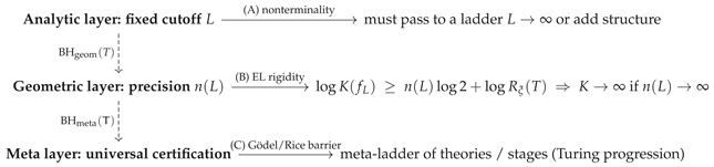
Remark 55

(Why this is the right “bigger generalization”). The theorem is not about ξ alone; it is about aprogram architecture: inverse limits of finite stages along several independent refinement axes. Every new refinement axis (height window T, precision n, bandwidth A, spectral cutoff L, conductor Q, error tolerance ε, ...) can be treated as a new coordinate in a multi-parameter ladder. If each coordinate has a positive energy increment, then energy diverges along any cofinal path. This is the general mechanism behind the repeated appearance of “infinite splitting” and “energy obstruction” across analytic, geometric, and meta-logical layers.

23. Explicit Two-parameter III+ Ladder for $\zeta$ via $\xi$: stages $(T,n)$ and the Energy $E_{\xi }^{\left(n\right)}\left(T\right)$

23.1. Discrete Height Ladder and Precision Ladder

Recall $\xi \left(s\right)=\frac{1}{2}s(s-1){\pi }^{-s/2}\Gamma (s/2)\zeta \left(s\right)$ and that RH for $\zeta$ is equivalent to “all zeros of $\xi$ in $0<\Re s<1$ lie on $\Re s=\frac{1}{2}$”.

Fix a base height $T_0>1$ and define the dyadic height ladder

$$T_m:=T_0+2m,uadm\in .$$

(41)

(Using step size 2 matches the level-height decomposition $I_j=(2j-1,2j+1)$.)

Fix also the precision ladder $n\in$ (corridor tightening level).

For each pair $(m,n){\in }^2$, define the stage $(m,n)⟷(T_m,n).$ Define the coordinate successor operators

$${\Sigma }_T(m,n):=(m+1,n)(\mathrm{increase}\mathrm{height}\mathrm{window}),uad{\Sigma }_n(m,n):=(m,n+1)(\mathrm{tighten}\mathrm{corridor}).$$

(42)

We equip ² with the product partial order $(m,n)⪯(m^{\prime },n^{\prime }):⟺m\le m^{\prime }\mathrm{and}n\le n^{\prime }.$

23.2. Two-Parameter Energy

Assume the $\xi$-corridor system has been defined at each height $T_m$: active levels ${\mathcal{J}}_{\xi }\left(T_m\right)$, representative zeros ${\rho }_j\left(T_m\right)={\sigma }_j\left(T_m\right)+\mathrm{i}{t}_j\left(T_m\right)$, and corridor radius $r_{\xi }\left(T_m\right)>0$. For each precision n define the tightened target corridors $Q_{j,n}^{\mathrm{tgt}}\left(T_m\right)$ and admissible class ${\mathcal{F}}_{\xi }^{\left(n\right)}\left(T_m\right)$ as in the main text.

Define the two-parameter truncated Teichmüller energy

$$E(m,n):=E_{\xi }^{\left(n\right)}\left(T_m\right):=\underset{f\in {\mathcal{F}}_{\xi }^{\left(n\right)}\left(T_m\right)}{inf}logK\left(f\right)\in [0,+\infty ],uad(inf⌀:=+\infty ).$$

(43)

23.3. The Explicit Two-Parameter Lower Bound (Geometric Increment in n)

Define the dimensionless corridor ratio at height T by

$$R_{\xi }\left(T\right):={\displaystyle \frac{{\displaystyle \sum _{j\in {\mathcal{J}}_{\xi }\left(T\right)}\left(1-2{\sigma }_j\left(T\right)-2r_{\xi }\left(T\right)\right)}}{{\displaystyle |{\mathcal{J}}_{\xi }\left(T\right)|·2r_{\xi }\left(T\right)}}}\in (0,+\infty ),$$

(44)

with the convention that $R_{\xi }\left(T\right)$ is undefined when ${\mathcal{J}}_{\xi }\left(T\right)=⌀$. (When ${\mathcal{J}}_{\xi }\left(T\right)\ne ⌀$, Lemma (Positivity of source corridor widths) implies $R_{\xi }\left(T\right)\ge 3$.)

Theorem 29

(Two-parameter explicit inequality for $E_{\xi }^{\left(n\right)}\left(T_m\right)$). Fix $m\in$ and assume ${\mathcal{J}}_{\xi }\left(T_m\right)\ne ⌀$. Then for every $n\in$,

$$E(m,n)=E_{\xi }^{\left(n\right)}\left(T_m\right)\ge nlog2+log{R}_{\xi }\left(T_m\right).$$

(45)

In particular, for each fixed m one has $E(m,n)⟶+\infty (n\to \infty ),$ so exact axis landing (the formal limit $n\to \infty$) is an infinite-energy boundary phenomenon at every fixed height window $T_m$.

Proof. 

This is exactly the $\xi$–tightening extremal-length lower bound specialized at $T=T_m$: at precision n, the target corridor widths are $2^{-n}\left(2r_{\xi }\left(T_m\right)\right)$, so modulus ratios force $K\left(f\right)\ge 2^n{R}_{\xi }\left(T_m\right)$ for every $f\in {\mathcal{F}}_{\xi }^{\left(n\right)}\left(T_m\right)$. Taking log and infimizing gives (45). □

23.4. Two Explicit Increments Along the Stage Lattice (a Genuine “III+” Form)

Define the lower-envelope energy at stage $(m,n)$ by

$$\underline{E}(m,n):=nlog2+log{R}_{\xi }\left(T_m\right).$$

(46)

Then Theorem 29 says $E(m,n)\ge \underline{E}(m,n)$.

The envelope $\underline{E}$ has explicit additive successor increments:

$$\underline{E}\left({\Sigma }_n(m,n)\right)-\underline{E}(m,n)=log2,uad\underline{E}\left({\Sigma }_T(m,n)\right)-\underline{E}(m,n)={\Delta }_T\left(m\right),$$

(47)

where

$${\Delta }_T\left(m\right):=log\left({\displaystyle \frac{R_{\xi }\left(T_{m+1}\right)}{R_{\xi }\left(T_m\right)}}\right).$$

(48)

Thus $(m,n)\mapsto \underline{E}(m,n)$ is a fully explicit two-parameter “III+” ladder: one coordinate has a constant increment $log2$, and the other has an explicit increment ${\Delta }_T\left(m\right)$ governed entirely by the corridor ratio data at successive height windows.

Remark 56 (A clean sufficient condition for astricttwo-increment III+ regime)If there exist constants $m_{*}\in$ and $\Lambda >1$ such that $R_{\xi }\left(T_{m+1}\right)\ge \Lambda R_{\xi }\left(T_m\right)uad\mathrm{for}\mathrm{all}m\ge m_{*},$ then ${\Delta }_T\left(m\right)\ge log\Lambda >0$ for all $m\ge m_{*}$, and hence $E(m,n)\ge \underline{E}(m,n)\ge \underline{E}(m_{*},0)+(m-m_{*})log\Lambda +nlog2uad(m\ge m_{*},n\ge 0).$ In this regime energy diverges alongeitherrefinement axis ($m\to \infty$ or $n\to \infty$), and along any cofinal path in².

23.5. Optional: Successor Permission in the n Direction (Upper Increment)

When the disc-preserving tightening maps exist (as constructed earlier, for $n\ge 1$), one also has an upper increment bound in the precision direction.

Proposition 5

(Successor permission for n (for $n\ge 1$)). Fix $m\in$ and assume ${\mathcal{J}}_{\xi }\left(T_m\right)\ne ⌀$. Then for every $n\ge 1$, $E(m,n+1)\le E(m,n)+log2,d_{\xi }^{(n+1)}\left(T_m\right)\le d_{\xi }^{\left(n\right)}\left(T_m\right)+\frac{1}{2}log2,$ provided $E(m,n)<\infty$ (i.e. ${\mathcal{F}}_{\xi }^{\left(n\right)}\left(T_m\right)\ne ⌀$).

Proof. 

Compose any near-minimizer $f\in {\mathcal{F}}_{\xi }^{\left(n\right)}\left(T_m\right)$ with the explicit disc-preserving tightening map $G_{T_m,n}$ of dilatation 2 on the target side. The composition lies in ${\mathcal{F}}_{\xi }^{(n+1)}\left(T_m\right)$ and has dilatation at most $2K\left(f\right)$, hence adds at most $log2$ to $logK$. □

23.6. Stage Diagram

[row sep=large,column sep=huge] (m,n) [r,"&#x003A3;n"] [d,"&#x003A3;T"’] (m,n+1)

(m+1,n) [r,"&#x003A3;n"’] (m+1,n+1)

On the explicit lower envelope $\underline{E}(m,n)=nlog2+log{R}_{\xi }\left(T_m\right)$, the ${\Sigma }_n$–increment is exactly $log2$ and the ${\Sigma }_T$–increment is ${\Delta }_T\left(m\right)=log(R_{\xi }\left(T_{m+1}\right)/R_{\xi }\left(T_m\right))$.

Remark 57

(How this specializes the III+ trichotomy to $\zeta$). The inequality (45) is the fully quantified “geometric clause” of the III+ trichotomy, specialized to the Riemann zeta function via its completion ξ: tightening precision n forces Teichmüller energy to increase at least linearly in n.

The “analytic clause” (finite-resolution nonterminality) is orthogonal to (45): it says that any strategy claiming to decide RH from a fixed cutoff using finitely many probes is nonterminal and must pass to a resolution ladder (a different coordinate). If one posits a bridge mapping analytic resolution to geometric tightening $L\mapsto n\left(L\right)$, then (45) converts that analytic ladder into a Teichmüller energy ladder automatically.

References

- Abikoff, W. The Real Analytic Theory of Teichmüller Space. In Lecture Notes in Mathematics; Springer-Verlag: Berlin–New York, 1980; Vol. 820. [Google Scholar]
- Adem, A.; Leida, J.; Ruan, Y. Orbifolds and Stringy Topology. In Cambridge Tracts in Mathematics; Cambridge University Press: Cambridge, 2007; Vol. 171. [Google Scholar]
- Ahlfors, L. V. Lectures on Quasiconformal Mappings . In University Lecture Series, 2nd ed.; American Mathematical Society: Providence, RI, 2006; Vol. 38. [Google Scholar]
- Ahlfors, L. V. Conformal Invariants: Topics in Geometric Function Theory . In McGraw–Hill Series in Higher Mathematics; McGraw–Hill Book Co.: New York; AMS Chelsea Publishing: Providence, RI, 1973. [Google Scholar]
- Ahlfors, L. V.; Beurling, A. The boundary correspondence under quasiconformal mappings. Acta Math. 1956, 96, 125–142. [Google Scholar] [CrossRef]
- Ahlfors, L. V.; Sario, L. Riemann Surfaces . In Princeton Mathematical Series; Princeton University Press: Princeton, NJ, 1960; Vol. 26. [Google Scholar]
- Astala, K.; Iwaniec, T.; Martin, G. Elliptic Partial Differential Equations and Quasiconformal Mappings in the Plane . In Princeton Mathematical Series; Princeton University Press: Princeton, NJ, 2009; Vol. 48. [Google Scholar]
- Bott, R.; Tu, L. W. Differential Forms in Algebraic Topology . In Graduate Texts in Mathematics; Springer-Verlag: New York–Berlin, 1982; Vol. 82. [Google Scholar]
- Conrey, J. B. The Riemann hypothesis. Notices Amer. Math. Soc. 2003, 50(no. 3), 341–353. [Google Scholar]
- Davenport, H.; Montgomery, H. L. Multiplicative Number Theory, revised and with a preface by. In Graduate Texts in Mathematics, 3rd ed.; Springer-Verlag: New York, 2000; Vol. 74. [Google Scholar]
- Edwards, H. M. Riemann’s Zeta Function . In Pure and Applied Mathematics; Academic Press: New York–London, 1974; Vol. 58. [Google Scholar]
- Gardiner, F. P.; Lakic, N. Quasiconformal Teichmüller Theory . In Mathematical Surveys and Monographs; American Mathematical Society: Providence, RI, 2000; Vol. 76. [Google Scholar]
- Haefliger, A. Groupoïdes d’holonomie et classifiants. Astérisque 1984, 116, 70–97. [Google Scholar]
- Hubbard, J. H. Teichmüller Theory and Applications to Geometry, Topology, and Dynamics . In Teichmüller Theory; Matrix Editions: Ithaca, NY, 2006; Vol. 1. [Google Scholar]
- Imayoshi, Y.; Taniguchi, M. An Introduction to Teichmüller Spaces; Springer-Verlag: Tokyo, 1992. [Google Scholar]
- Ivić, A. The Riemann Zeta-Function: Theory and Applications; originally published by; Dover Publications: Mineola, NY; John Wiley & Sons, 2003. [Google Scholar]
- Iwaniec, H.; Kowalski, E. Analytic Number Theory . In American Mathematical Society Colloquium Publications; American Mathematical Society: Providence, RI, 2004; Vol. 53. [Google Scholar]
- Katok, A.; Hasselblatt, B. Introduction to the Modern Theory of Dynamical Systems . In Encyclopedia of Mathematics and its Applications; Cambridge University Press: Cambridge, 1995; Vol. 54. [Google Scholar]
- Kawasaki, T. The index of elliptic operators over V-manifolds. Nagoya Math. J. 1981, 84, 135–157. [Google Scholar] [CrossRef]
- Lehto, O.; Virtanen, K. I. Quasiconformal Mappings in the Plane . In Grundlehren der Mathematischen Wissenschaften, 2nd ed.; Springer-Verlag: New York–Heidelberg, 1973; Vol. 126. [Google Scholar]
- Moerdijk, I.; Pronk, D. A. Orbifolds, sheaves and groupoids. K-Theory 1997, 12(no. 1), 3–21. [Google Scholar] [CrossRef]
- Nag, S. The Complex Analytic Theory of Teichmüller Spaces. In Canadian Mathematical Society Series of Monographs and Advanced Texts; John Wiley & Sons, Inc.: New York, 1988. [Google Scholar]
- Riemann, B. Über die Anzahl der Primzahlen unter einer gegebenen Grösse. Monatsberichte der Königlichen Preussischen Akademie der Wissenschaften zu Berlin 1859, 671–680. [Google Scholar]
- Satake, I. On a generalization of the notion of manifold. Proc. Natl. Acad. Sci. USA 1956, 42, 359–363. [Google Scholar] [CrossRef] [PubMed]
- Strebel, K. Quadratic Differentials . In Ergebnisse der Mathematik und ihrer Grenzgebiete (3); Springer-Verlag: Berlin, 1984; Vol. 5. [Google Scholar]
- Thurston, W. P. The Geometry and Topology of Three-Manifolds . Princeton University Lecture Notes. 1979. Available online: http://library.msri.org/books/gt3m/.
- Titchmarsh, E. C. The Theory of the Riemann Zeta-Function, 2nd ed.; Heath-Brown, D. R., Ed.; Oxford Science Publications, Clarendon Press, Oxford University Press: Oxford, 1986. [Google Scholar]
- Väisälä, J. Lectures on n-Dimensional Quasiconformal Mappings . In Lecture Notes in Mathematics; Springer-Verlag: Berlin–New York, 1971; Vol. 229. [Google Scholar]
- Vuorinen, M. Conformal Geometry and Quasiregular Mappings. In Lecture Notes in Mathematics; Springer-Verlag: Berlin, 1988; Vol. 1319. [Google Scholar]
- Warner, F. W. Foundations of Differentiable Manifolds and Lie Groups . In Graduate Texts in Mathematics; Springer-Verlag: New York, 1983; Vol. 94. [Google Scholar]
Disclaimer/Publisher’s Note: The statements, opinions and data contained in all publications are solely those of the individual author(s) and contributor(s) and not of MDPI and/or the editor(s). MDPI and/or the editor(s) disclaim responsibility for any injury to people or property resulting from any ideas, methods, instructions or products referred to in the content. |
© 2026 by the authors. Licensee MDPI, Basel, Switzerland. This article is an open access article distributed under the terms and conditions of the Creative Commons Attribution (CC BY) license (http://creativecommons.org/licenses/by/4.0/).
Copyright: This open access article is published under a Creative Commons CC BY 4.0 license, which permit the free download, distribution, and reuse, provided that the author and preprint are cited in any reuse.