
Submitted:
09 January 2026
Posted:
12 January 2026
You are already at the latest version
Abstract
Water shortage is a major problem that affects sustainability of agricultural sector in northeastern Thailand especially areas remote from a main river. This study aims at developing a system for water shortage risk assessment at sub-district level in Maha Sarakham Province. QSWAT model for sub-watershed streamflow simulation was integrated with WEAP model to analyze water balance and assess water shortage based on water demand from five sectors: non-irrigated agriculture, irrigated agriculture, consumption, services, and industry. The findings revealed that both models provided the results of calibration, and the validated results of streamflow analysis were at satisfactory to good level. From spatial analysis, distribution of provincial water resource was significantly different. Sub-districts located along the Chi River had high streamflow but low water shortage while those from central to southern part had limited streamflow although water demand was high especially for agricultural sector. According to temporal analysis, critical period of water shortage was found in the dry season and seasonal transition after post-harvest period. Integration of data on streamflow and water demand can be useful to divide subdistricts into three group: positive water balance, balance, and negative water balance. Most sub-districts were classified as negative water balance that needed urgent measures for water resource development. These findings have provided important data for planning water resource management locally and supporting development of drought mitigation measures for vulnerable areas in Maha Sarakham Province.
Keywords:
hydrological modeling
; drought vulnerability
; seasonal variation
; Chi River Basin
; agricultural water demand
; decision support system
; GIS-based risk assessment
1. Introduction
Climate change has significantly affected hydrologic cycles and water resource management over the past decade. Particularly, an increase in global average temperature leads to the changes in rainfall, runoff, and increased evaporation rate [1]. These changes cause higher severity of water-related disasters especially unusual prolonged drought in many regions around the world during 2020-2023 [2]. Impact assessment and a plan for coping with the climate change require a numeric model with high precision to simulate hydrological processes and prediction of global changes [3,4]. Southeast Asia is one region that has been most significantly affected by the climate change. Cambodia, Vietnam, and Laos, in particular, has been affected by the drought during 2020-2022, impacting region’s agricultural productivity and food security [5]. Water management in this region is complicated since both physical and socioeconomic factors have to be considered. As a result, models for hydrologic and water management become more attracted [6], and this results in the development of decision support system integrating several models for systematic problem analysis and strategic planning in water management [3,7].
Thailand has experienced severe drought over the past decade, especially the Northeast where agriculture is damaged over 15,000 million Baht in 2022 [8,9]. Applying hydrologic models to water prediction and management planning is unlimited in Thailand [10]. Most of the previous studies have tried to use single models for problem analysis, such as using hydrologic models to assess the impacts of land use changes on the runoff in the Northeast [11], using water budget models to analyze water demand in the Chao Phraya River Basin [12]. However, studies on integration of several models are not sufficient although the potential of problem analysis is high [7]. Moreover, those studies emphasize watershed or province level analysis, so the analysis at smaller level for supporting local planning is still lacking [13]. Development of spatial water assessment and monitoring system is important to improving the efficiency of country’s water resource management [6], especially a system to support decision making at local level integrating with national water management system [7,14]. Integrating hydrologic model technology with geographic information system is essential for decision support system development on future water management [15].
Currently, spatial model is employed in situational analysis of water because it can display geospatial and temporal data to support stakeholders to have more understanding of situations easily [16]. Integration between hydrologic model and water budget model is more widely used in many regions throughout the world for spatial water prediction. In Cambodia, for example, Touch et al. [17] used both of these models to assess the impacts of urban development on water security in the Tonle Sap Lake Tributary Basin. The study of Tran et al. [16] shows the quality of water management planning for semi-arid areas in Cuba. Also, in Vietnam, Khoi et al. [18] applied both mentioned model to assess water scarcity risk at sub-basin level in Vietnam.
One of the hydrologic models globally used for hydrologic analysis in river basins is SWAT because it can be used to simulate complicated hydrologic processes at sub-watershed level [19]. A study conducted by Bal et al. [20] demonstrates that SWAT can be used to simulate the impacts of land use changes in India on runoff precisely. This is consistent with a study conducted in Turkey by Aibaidula et al. [21] using SWAT to analyze the effects of climate change on reservoir water storage volume. In Ethiopia, Eshete et al. [22] used SWAT to analyze water scarcity risk in drought-prone areas. The important advancement of SWAT is that it was developed into a public domain model that can help researchers develop their model without financial constraints. This can lead to the integration of Quantitative Soil and Water Assessment Tool (QSWAT) [23,24,25] and Quantum Geographic Information System (QGIS) [25,26] to increase capacity in spatial analysis. Currently, QSWAT has been widely used for hydrologic model development in Southeast Asia, such as an analysis related to the effects of climate change on rained-dependent agricultural sites in Asia conducted by Goswami et al. [27], a study on geospatial and temporal hydrologic elements in a basin at regional level in Thailand [28,29,30], and potential assessment of water resources for dry-season crop cultivation planning [31].
Also, Water Evaluation and Planning System (WEAP) is a model widely used because it has the strengths in analyzing water balance and water scarcity in a drought-prone area, and it has been widely applied in many regions both in historic-present and future [32,33]. In South Africa, WEAP was utilized by Al-Mukhtar and Mutar [34] to analyze water allocation for different sectors in dry season while Ben Salem et al. [35] applied it to irrigation system and water scarcity risk assessment in drought-prone areas in Morocco. In the context of Southeast Asia, WEAP is also commonly used. In Vietnam, for example, the research conducted by Dau et al. [36] applied it to the water scarcity risk assessment for irrigated area in the Mekong Delta. In Thailand and Southeast Asia, Kuntiyawichai and Wongsasri [37] assessed the impacts of drought on water security at community level while Forni et al. [38] and Guzman et al. [39] developed a decision support system for water management in agricultural sites with water scarcity risk in Cambodia and Philippines, focusing on community participation in water utilization planning.
However, the previous studies lack small-scale spatial analysis, especially at local government organization level [40,41]. The study conducted by Candido et al. [42] and Nagata et al. [43] report the challenges of the development of output system that is easily understood by local users. Thailand has encountered several constrains in local water management, such as a lack of efficient tools for analyzing and forecasting water situation and limited data sharing between central and local government organizations, which cause inefficiency in local drought management. Therefore, this research emphasizes integration of QSWAT and WEAP models to solve these mentioned constrains through a developed sub-district level water scarcity risk assessment that can display the output in clear maps and graphs. Moreover, an open-source model was used for system modification to fit the local context. Integration of both models also increase capacity in hydrologic analysis and water resource management [33], which are essential for water management planning in drought-prone areas in Thailand.
This study aims to integrate QSWAT and WEAP models for sub-district level water scarcity risk assessment in Maha Sarakham Province, which is regarded as a drought-prone area in the Chi River watershed, northeastern Thailand. Maha Sarakham has repetitively faced severe drought over the past decade, especially in a prolonged dry season that agricultural sector is affected. Although the Chi River is the major water resource in this province, allocation of water into remote areas is limited because agricultural sites and communities have been expanded. As a result, QSWAT-WEAP integration is the key to systematic water situation analysis in a drought-prone area particularly in considering streamflow at sub-watershed level using QSWAT together with assessing sub-district level water scarcity risk using WEAP. Furthermore, this study focuses on developing decision support system that can display clear maps of sub-district level water scarcity risk in order that local government organizations and stakeholders can use it as a tool for planning their drought solutions in drought-prone areas, where water demand is high but water source is limited.
The result of this study can be useful for any agencies responsible for water management and drought solution at both policy and operational levels, such as Office of the National Water Resources, Royal Irrigation Department, and Local Government Organization, in order to assess water scarcity risk and establish mitigation measures for drought-prone areas. The displayed output of low risk can allow local administrators and officers to understand situations and provide high efficiency of resource allocation policy especially in Maha Sarakham, where water management for drought-prone area is very challenging. Integrating QSWAT and WEAP models with Geographic Information System (GIS) can improve the precision of analysis and forecast of water scarcity risk. Farmers and water consumers can utilize data from this system for their cultivation planning and water consumption aligned with water source available at each time period. In addition, the methodology of the study can serve as a model for system development of water scarcity risk assessment in other drought-prone areas, where water allocation is limited and water demand is various.
2. Materials and Methods
2.1. Study Area
2.1.1. Hydrological Characteristics of the Study Area
The study area is within the Chi-Mun Rivers system in northeastern Thailand (see Figure 1) including diverse topographic features but mostly the Korat Plateau with elevation from 193 to 371 meters above mean sea level (MSL). On the western side, the topographic features include mountains in Phetchabun Province with elevation from 729 to over 1,622 meters above MSL. Its hydrologic network is composed of two main rivers including the Chi River, where its source is from a western mountainous area, and the Mun River, which flows through the southern part of area. Additionally, it consists of two large reservoirs; Ubolrat and Lam Pao Reservoirs, which help control streamflow in the watershed. There is also a network of six meteorological monitoring stations (E.22B, E.91, E.9, E.66 and M.95) strategically distributed throughout the watershed to monitor spatial variability of flow patterns. Diverse physical features and comprehensive inspection network of this area become significantly reasonable to develop hydrologic modeling by using QSWAT.
2.1.2. Administrative Boundaries and Adjacent Areas
The major study area is Maha Sarakham Province including 5,292 square kilometers (sq.km) located in a strategic location, where several tributaries within the Chi-Mun system joining together. The Province borders Khon Kaen Province to the north, Roi Et Province to the east, and Surin Province to the south. It consists of 133 sub-districts, and each of them is clearly defined boundaries for systematic assessment and water resource management. Nevertheless, this study area also extends into the adjacent provinces which are part of the watershed to ensure that the hydrologic system is fully covered. Administrative boundaries serve as fundamental units to implement water management and availability assessment of water at sub-district level.
2.2. Hydrologic Modeling
2.2.1. QSWAT Model
QSWAT, which integrates Soil and Water Assessment Tool (SWAT) with QGIS, is a comprehensive hydrologic model system designed to simulate hydrologic processes at watershed level [19]. This integrated model was developed to increase capacity in accessing hydrologic analysis, and it has been extensively applied in different fields as well as fluid dynamics assessment, sediment yield analysis, and analysis of impacts of land use and climate change on water resource [20,21,22,28,29,30]. The model depends on hydrologic foundation using water balance equations calculating change in storage as component difference of flow in and out, and it also uses energy balance approach for evapotranspiration modeling. The latest application demonstrates diverse models in different geographic and hydrologic contexts as well as runoff and erosion assessment [44,45], flood risk model development [46,47], efficiency improvement of watershed management [48] emphasizing potential of the model in its accuracy and adaptability. Water balance in QSWAT is shown in Equation (1).
where SWtotal is soil water content at time t (mm); SW0 is initial soil water content (mm); t is time in day unit; Rd is daily cumulative rainfall on day i (mm); Qs is cumulative runoff on day i (mm); Ea is actual evapotranspiration on day i (mm); wseep is infiltration on day i (mm); Qgw is groundwater content on day i (mm).
2.2.2. Data Collection
2.2.3. Sub-Basin Delineation
The study area is located in Maha Sarakham Province covering one part of all Chi and Mun Basins. The Chi Basin has four sub-watersheds including Chi Watershed 3, Chi Watershed 4/1, lower Phong Watershed 2, and Lower Lam Pao Watershed. For sub-watershed division in QSWAT of the Chi watershed, source of the Chi River and Ubolrat Reservoir’s catchment area have to be considered. The Mun Basin also has four sub-watersheds including Lam Siao Yai Watershed 1, Lam Phang Chu Watershed, Lam Plapphla Watershed, and Lam Tao Watershed. All of them are tributaries of the Mun River. In QSWAT, however, division of additional sub-watersheds for the Mun Watershed is unnecessary. Sub-watershed in QSWAT integrates DEM data with available stream network data. This process results in attaining 90 watersheds in Maha Sarakham Province, which is consistent with sub-district administrative boundary as shown in Figure 1.
2.2.4. Importing Rainfall and Meteorological Data
QSWAT is calibrated and validated using rainfall and meteorology data covering divided sub-watersheds as mentioned in 2.1.1. data obtained from the Thai Meteorological Department (TMD) and the Hydro - Informatics Institute (HII) include station 111 rainfall monitoring stations, 34 temperature monitoring station (minimum and maximum), 34 relative humidity monitoring stations, 8 wind speed monitoring stations, and 5 solar radiation monitoring stations. The 14-year daily data are analyzed (2010 - 2023). Spatial distributions of meteorological variables for each sub-watershed are identified by Thiessen polygon method as shown in Figure 2.
2.2.5. Importing Hydrologic Response Units
Generally, all watershed areas are different in land use, soil types, slope, and land management. A watershed area probably has more than one type of land use, or it uses different ways of land management for each plant depending on soil type and land slope [20]. Each part of the watershed has its own hydrologic parameters, such as curve number (CN) based on land use and soil type, which can lead to different hydrologic outcomes [49].
For this study, QSWAT employed a spatial analysis tool in QGIS importing two layers of GIS data, i.e., land use data in 2019 and soil series data in 2015 recorded by the Land Development Department (LDD). These imported data were overlaid in order to gain new data layers. The new layers in each boundary were from the intersection of two-layer data, referred to as Hydrologic Response Units (HRUs). Each HRU can be imported different hydrologic parameters. This calculation can give more details and reliability to the model. This study land use data were imported by land use type based on land use code in QSWAT database, totaling 19 types while the imported soil series types were defined by code in QSWAT database, totaling 41 types. Then the two-layer data spatially overlaid by QSWAT resulted in the attainment of 414 HRUs. The details of land use map and soil series inputs for the model are presented in Figure 3 (a) and (b).
2.3. WEAP Model
Water Evaluation and Planning System (WEAP) model was developed by Stockholm Environment Institute (SEI) in 1988. It serves as an integrating tool for water resource planning and assessment [32]. The model requires basic data regarding hydrology, meteorology, water resources, water demand, and water infrastructure in the study area. WEAP has been globally used because of its capacity in simulating complex system of water resource, analyzing water management policy, and simulating to assess water management options. Model’s flexibility allowed parameters and conditions to be adaptable for assessing the impacts of climate change, land use change, and water infrastructure development in order to analyze priority-based water allocation as well as water scarcity risk assessment by sector [32,33,34,35,36,37,38,39]. WEAP can be integrated with other hydrologic models, such as SWAT, using the result of streamflow simulation as water resource data for water balance analysis and scarcity assessment [33,50,51]. Moreover, compatibility with groundwater model and water quality can lead to comprehensively quantitative and qualitative analysis as well as higher precision and reliability of the results.
WEAP uses four basic equations for water balance modeling and water scarcity analysis [37], including Equation (2): mass balance for water volume change in a system, Equation (3): water balance at the node for storage volume change, Equation (4): water demand calculation inclusive of efficiency and area, and Equation (5): water scarcity specified by difference between demand and supply as follows:
where dV/dt is rate of water volume change rate per time system; Qin is water volume flowing into system; Qout is water volume flowing out system; S(t+1) and S(t) is storage volume at time t+1 and t respectively; I(t) is water content flowing in at time t; O(t) is water content flowing out at time t; WD is water demand; AWR is rate of water demand per unit of area; ef is water use efficiency; AL is water consuming area; WS is water scarcity
WEAP requires three main types of input: 1) water supply, 2) spatial data, and 3) water demand data (Table 2), including seven components: 1) demand site node, 2) flow requirement node, 3) reservoir node, 4) river, 5) transmission link, 6) return flow, and 7) streamflow gauge. Imported GIS data as the background of model include watershed boundary, river network, water source, streamflow gauge, irrigation area, road, and sub-district boundary as seen in Figure 4 and Figure 5, respectively.
2.4. Model Performance Assessment
Efficiency of QSWAT and WEAP models were assessed by three statistical indices. For the assessment, QSWAT used Coefficient of Determination (R²) to identify the relationship between measured and modeled streamflow values (Equation 6), Nash-Sutcliffe Efficiency (NSE) to measure model’s forecast precision compared to observed mean (Equation 7), and ratio of RMSE to standard deviation of observed values (RSR) (Equation 8). The assessment covered the whole phase of calibration (2010-2016) and validation (2017-2023) - each of them spanned 7 years.
On the other hand, WEAP utilized simulation results obtained from QSWAT as its inputs. The efficiency assessment emphasized R² and NSE values since they have been normally used for precision assessment of streamflow simulation in the water balance model. The results obtained from simulation were compared to the measured data during a 14-year period (2010-2023). The study used statistically reliable criteria for calibrating monthly model to assess its precision and accuracy [52]:
where Oi is streamflow content recorded at the streamflow gauge; Ō is average streamflow content recorded at the streamflow gauge; Pi is streamflow content calculated by QSWAT and WEAP; is average streamflow content calculated by QSWAT and WEAP; i is data sequence
2.5. QSWAT-WEAP Framework for Water Balance Simulation
According to the concept of water balance assessment by developing integrated QSWAT-WEAP model (see Figure 6-Framework for water balance assessment), the study included both supply and demand sides. The supply side consists of streamflow content simulation of QSWAT that required important inputs, such as DEM, land use, river network, soil type, sub-watershed boundary, meteorological data, reservoir specifications, data regarding storage capacity, storage curve, and evaporation rate, and operational rules. These data were processed in QSWAT to simulate streamflow for each sub-watershed. On the other hand, the demand side, as seen in the upper part of Figure 6, comprises water demand in four sectors, i.e., industry, consumption, agriculture (both irrigated and non-irrigated areas), and services. These sectors were calculated as water demand combined with spatial data including water source, administrative boundary, watershed boundary, irrigation zone, and streamflow gauge location for water balance simulation in WEAP.
The simulation results from WEAP demonstrating on the right side created 4 major spatial outcomes at sub-district level including 1) sub-district streamflow, 2) water demand, 3) water shortage, and 4) level of water shortage. These outcomes were presented through spatial distribution to support decision making on water management and water allocation planning at sub-district level.
3. Results and Discussions
3.1. Streamflow Simulation from QSWAT
3.1.1. Parameter Sensitivity Analysis
Sensitivity analysis of parameters for QSWAT was conducted using SWAT-CUP through Sequential Uncertainty Fitting version 2 (SUFI2) [53] to analyze parameters related to the streamflow calculation in the model compared to 14-year (2010-2023) monthly streamflow data of six monitoring stations. Optimization to obtain comparable results to measured value was 300 iterations by selecting 14 parameters affecting the streamflow [28] and defining Nash-Sutcliffe (NSE) as an objective function. The result of global sensitivity analysis from SWAT-CUP was expressed through t-Stat and p-Value obtained from hypothesis testing of a relationship between parameters and objective function. This analysis indicated that the leading three parameters affecting calculation result were GWQMN (3537), SOL_AWC (0.07), and GW_REVAP (0.83). In analyzing absolute values of t-Stat and p-Value approaching zero, it indicated significant sensitivity to objective function [54]. The remaining 11 parameters with low sensitivity were ranked and presented in Table 3.
3.1.2. Performance Assessment of Models
The result of performance assessment of QSWAT and WEAP models are illustrated in Figure 7, which presents heat map indices, and Figure 8, which represents the consistency of monthly streamflow data from monitoring stations and the calculation results gained from time series model of six stations during 2010-2023. According to the result from QSWAT during calibration period (2010-2016), most stations had R2 between high and very high level (0.66–0.87). Station E.66 had the highest level (0.87). NSE was between 0.14 and 0.83; station E22B and Ubolrat Reservoir (Inflow UB) had variation below satisfactory range (at 0.14 and 0.46, respectively). The period of low streamflow was noticed at both stations. The values obtained from the models were higher than the observed values as shown in Figure 8 (b) and 8 (c); however, based on the average of all six stations, NSE was at satisfactory level (0.58). RSR index was consistent with NSE (0.63), which was satisfactory. In the period of model validation (2017-2023), each index showed better outcomes. Stations E9, E91, and E66 indicated their results at very good level from three indices. The remaining stations were at good and satisfactory levels represented by the average of R2 = 0.72, NSE = 0.70, and RSR = 0.54.
Performance assessment of streamflow simulation using WEAP was to reverify the calculation results of streamflow gained from QSWAT. In WEAP context, the streamflow of main river, which flows through the study area and become potential and applicable, has led to water balance analysis for three parts: 1) water availability, 2) water demand, and 3) sub-district level water shortage in Maha Sarakham Province. In assessment, R2 and NSE indices were used focusing on four main stations (E.9, E.91, E.66A, and M.95). The first three stations aimed to monitor streamflow in the Chi River affecting northern Maha Sarakham Province. On the other hands, M.95 needed performance assessment for Lam Siao River located in the South outside Maha Sarakham Province area. This study found that WEAP was able to simulate streamflow and had R2 between 0.66 and 0.80 and NSE between 0.65 and 0.71, compared to four monitoring stations, and had consistency of temporal data during 2010-2023 as presented in Figure 8 (a), (d), (e), and (f). The average of both indices was at good level, and the optimal models ranked by performance were E.9, E.91, E.66, and M.95. The overall performance assessment for QSWAT and WEAP supported that streamflow stimulated by both models provided reliable data from satisfactory to good level compared to model standard and temporal data consistency.
3.2. Spatial Distribution of Water Resources
3.2.1. Sub-District Streamflow Analysis
The results of streamflow analysis in QSWAT and WEAP during 2010-2023 shown in Figure 9 (a) were classified into five levels of spatial distribution. Sub-districts located near the Chi River, which is a main river flowing through northern and central parts of the province (represented by the dark blue in the map), demonstrated high to very high streamflow (Ranges 4-5: 250-7,600 MCM per year) due to surface runoff over sub-district area and influence of water from the main river. On the other hand, southern and southwestern sub-districts in the province (represented by the light green), which is far from the main river and relies only on surface runoff in the area, had low streamflow (Range 1: 2-40 MCM per year). From analyzing quantitative data (see Figure 9 (b)), Range 1 covers 2,212 sq.km or 46% of the total area including 66 sub-districts while Range 5 covers only 359 sq.km or 8% of the total area including 7 sub-districts. For Range 2-4, it covers 2,521 sq.km or 47% including 59 sub-districts (40, 16, and 3 sub-districts respectively) distributing in central part of the province, which is a border area between the main river and areas remote from the river.
The analysis of monthly streamflow changes as shown in Figure 9 (c) and 9 (d) revealed seasonal changes consistent with spatial distribution in Figure 8(a). Ranges 1-3 (Figure 9 (c)) had low streamflow; maximum during September – October with 4.2 - 42.7 MCM streamflow and minimum during February – April with 0.02-0.28 MCM streamflow. This is related to the light yellow, light green, and light blue areas in the distribution map covering 122 sub-districts or 91% of the total sub-districts. In case of Ranges 4-5 as shown in Figure 9 (d), the maximum streamflow was 1,665.5-1,750.3 MCM in October, and the average streamflow in the dry season (December - July) was 94.3-555.6 MCM, which is in line with light and dark blue areas in the map of distribution along the Chi River.
According to the analysis of spatial streamflow distribution corresponding to area size, the number of district, and monthly temporal changes in Maha Sarakham Province, the study found seasonal imbalance and limited streamflow in the dry season. In contrast, intensity became high in the rainy season, which was significantly consistent with spatial contribution and geographical characteristics of Maha Sarakham Province. In the dry season, the areas with 0 – 100 MCM per year streamflow (Ranges 1-2) covering 2,047 sq.km area (78% of the total area) including 106 sub-districts (out of 133 sub-districts) indicated low monthly streamflow that reflected widespread distribution of sub-district level drought. For the central area (100 – 250 MCM per year), it included 709 sq.km or 13% of the total area. The areas with high streamflow (250 - 7,600 MCM per year), which are mostly located near the Chi River covering 489 sq.km including only 11 sub-districts, obviously showed higher value from June to October. This imbalance reflets that the area between central and southern parts had low level of monthly streamflow change while there were not many northern sub-districts having very high intensity of streamflow in the rainy season. Significant difference of streamflow between areas close to and far from the main river reflects a key role of the Chi River in being a major water resource of the province as well as influence of Ubolrat Reservoir to control the streamflow in the dry season. It is consistent with the findings of He et al. [55] indicating that the areas far from the main water resource in the Mekong watershed normally encounter water shortage, and the findings of Cheng et al. [56] highlighting that the distance from a main river is a factor to identify the availability of local water resources.
3.2.2. Sub-District Water Demand Analysis
Water demand at sub-district level through WEAP was analyzed based on five activities: non-irrigated agriculture, irrigated agriculture, consumption, services, and industry as shown in Figure 10 (a) and 10 (b), and it was also divided into five levels. Most of the sub-districts in the province were at level 1 of water demand (1 – 10 MCM per year) including 32 sub-districts and covering 903 sq.km or 17% of the total area, which distributed outside the province to the north and the east (represented by yellow). There were 98 sub-districts having medium level of water demand (Ranges 2 – 4: 10 – 40 MCM per year) covering 4,211 sq.km or 80% distributing in northern, central, and southern part of the province. The highest level of water demand (Range 5: 40 – 55 MCM per year) was found in only three sub-districts covering 178 sq.km or 3% (represented by dark purple in the map). An important notice from comparing between Figure 10 (a) and Figure 9 (a) is that water demand distribution is obviously different from streamflow distribution. In other words, the sub-districts where water demand is high do not need to be close to a main water resource, so this inconsistency becomes an important cause of water shortage for the areas remote to a main river.
Figure 10 (c) presents the change of monthly average water demand which is in line with local crop calendar. All sub-districts have water demand starting from June, which is the period of in-season rice cultivation. For the sub-districts with level 5 of water demand, they need 9.8 MCM water in August while those with Range 1 of water demand require 1.4 MCM water in the same month. During the dry season (January - May), areas of all levels have significantly lower water demand. The sub-districts with Range 1 have average water demand of 0.9 MCM per month. From analyzing the proportion of water demand by sector (Figure 10 (d)), non-irrigated agriculture shows the highest proportion at 1,713.5 MCM per year (88.7%), followed by irrigated agriculture at 185.8 MCM per year (9.6%), consumption at 18.9 MCM per year (0.98%), industry at 12.0 MCM per year (0.6%), and services at 2.6 MCM per year (0.13%). Figure 10 (e) demonstrates the trend of annual water demand, which has continually increased since 1981 from approximately 1,500 MCM to approximately 2,500-3,000 MCM in 2023, representing an average annual increase of 1.7%, caused by agricultural area expansion and population growth. The water demand proportion for non-irrigated agriculture increasing 88.7% reflects that local agriculturists are reliant mainly on rainfall, which is vulnerable to climate change. Considered in conjunction with Figure 9 (a), southern sub-districts in Maha Sarakham Province, where the streamflow is low, have moderate – high water demand (Ranges 2-4). This indicates the imbalance between demand and supply of water that can lead to water shortage.
3.3. Water Shortage Risk Assessment
3.3.1. Sub-District Water Shortage Analysis
Due to calculating the difference between water demand and available streamflow in each sub-district, sub-district level water shortage can be assessed as shown in Figure 11 (a) and classified into five ranges. There were 28 sub-districts having lowest water shortage (Range 1: 0-2 MCM per year) covering 980 sq.km or 19% of the total area. These sub-districts distribute over the north along the Chi River (represented by light yellow) influenced by high volume of streamflow (Ranges 4-5: 250-7,600 MCM per year). Figure 11 (b) presents 79 sub-districts with moderate water shortage (Ranges 2-3: 2-10 MCM per year) covering 3,172 sq.km or 60% of the total area distributing widely around central part of the province. There were 26 sub-districts facing severe water shortage (Ranges 4-5: 10-35 MCM per year) covering 1,140 sq.km or 22% of the total area distributing in the south and the southwest (represented by dark orange and red). These distributions represent the imbalance mentioned in Section 3.2.1 and Section 3.2.2; in other words, the southern area has low streamflow (Ranges 1-2: 2-100 MCM per year), but its water demand is at moderate to high level (Ranges 2-5: 10-55 MCM per year).
Figure 11 (c) and 11 (d) represent monthly change of water shortage obviously different from streamflow and water demand. The sub-districts with Range 1 as presented in Figure 11 (c) have low constant water shortage throughout the year. The maximum is 0.07 MCM in December while the minimum is 0.0 MCM in April, May, and October. The sub-districts with Ranges 2-5 as shown in Figure 11 (d) have maximum water shortage during November – December; 5.63 MCM in November for Range 5 followed by 2.85 MCM for Range 4. All ranges show the minimum in May (0.01-0.08 MCM), which is in the beginning of the rainy season. An interesting finding is that the critical period of water shortage (November - December) is not the highest water demand period (June - August) as described in Section 3.2.2. On the contrary, the streamflow rapidly decreases in post-harvest period while water is demanded for land preparation for the next cycle. This phenomenon indicates that seasonal transition is the critical period of water shortage in agricultural areas [57], and it suggests the importance of water allocation in order of priority during this critical period [58].
3.3.2. Sub-District Level of Water Shortage Analysis
Analyzing proportion of water shortage severity by percentage of unmet water demand receives more insightful answers than considering only absolute water shortage as described in Section 3.3.1 since the sub-districts with low water demand but high proportion of water shortage are probably affected higher than those with high water demand but low proportion of water shortage. Figure 12 (a) demonstrates five levels of severity classification. The sub-districts with high severity cover 1,664 sq.km or 31.4% including 40 sub-districts and distributing in the south and the east of the province (represented by orange). Secondly, sub-districts with medium severity cover 1,397 sq.km or 26.4% including 32 sub-districts and distributing in central part of the province. Figure 12 (b) shows the sub-districts with very high severity. Although it includes only 33 sub-districts, it covers 1,242 sq.km or 23.5% distributing in the southernmost and southwestern parts (represented by red), and overlapping with the areas with low streamflow (Ranges 1-2 in Section 3.2.1). On the other hand, there are only 28 sub-districts with very low to low severity covering 989 sq.km or 16% and distributing in the north along the Chi River.
Monthly severity changes as shown in Figure 12 (c) and 12 (d) reveal a critical situation for the areas with high and very high severity. The sub-districts with very high severity show 99.24% water shortage in March and the severity is still higher than 95% during January – April. It means that water demand has not been responded in the dry season although in the rainy season, the value is still at 35.23 - 51.80%, which is regarded as very high. The sub-districts with high severity show similar result; maximum = 96.82% in March while minimum = 4.96% in October, while those with medium severity have the maximum at 85.00% in March and the minimum at 0.79% in October. Those with very low severity have low and constant values throughout the year, and the maximum is only at 0.22% in June. The overall result indicates that there are 105 sub-districts or 79% of the total sub-districts (medium to very high) significantly affected by water shortage risk in terms of water use activities especially during January – April at all levels (except very low) with higher 50% water shortage. This result suggests that areas from central to southern part need urgent measures, such as minor water source development, promotion of water use efficiency, and cultivation planning based on water availability.
3.4. Synthesis of Water Balance and Shortage Risk Findings
The finding integration between distribution of water resources (Section 3.2) and water shortage risk assessment (Section 3.3) represents an obvious relationship between water supply and demand at sub-district level in Maha Sarakham Province. The study found the imbalance between available streamflow and water demand that was significantly different between the north and the south of the province. The northern area along the Chi River has high streamflow (Ranges 4-5: 250-7,600 MCM per year) covering 11 sub-districts and 489 sq.km (9%), and has very low to low severity of water shortage covering 28 sub-districts and 989 sq.km (18.7%). Conversely, from central to southern area has low streamflow (Ranges 1-2: 2-100 MCM per year) covering 106 sub-districts and 4,094 sq.km (78%), and has high to very high severity covering 73 sub-districts and 2,906 sq.km (54.9%). This difference was caused by the concentration of main water sources in the north while water demand distributed throughout the province; in other words, most sub-districts (101 sub-districts or 76%) had medium to high water demand (Ranges 2-5: 10-55 MCM per year) as shown in Table 4.
Based on temporal analysis, interesting findings on monthly water shortage were revealed. Section 3.3.1 has described that maximum water shortage was found during November – December; that is to say Range 5 area had maximum at 5.63 MCM in November. Section 3.3.2 has indicated that the areas with very high level had 99.24% water shortage in March and were higher than 95% during January – April, which means water demand was not met in the dry season. After considering sub-district characteristics of each risk level as presented in Table 5, sub-districts with very high risk had common characteristics, i.e., being located more than 25 km from a main river, streamflow intensity below 0.5 MCM per sq.km, and dependence on rainwater as a main water source, and the critical period was long from November to June. On the other hand, the sub-districts with very low risk were located near or within five km of the Chi River, and they had the streamflow intensity over 100 MCM per sq.km and benefited from the existing irrigation system. These characteristics indicate that a distance from the main river and irrigation system accessibility are factors for specifying risk level that can be used as criteria to screen target areas for future development of water sources. Overall, the findings support the necessary to develop minor water sources and local irrigation system in the south of the province as well as promotion of water use efficiency for non-irrigated agriculture, which needed high water demand at 88.7%.
4. Conclusions
Maha Sarakham Province is an important agricultural area in northeastern Thailand that has encountered persistent water shortage over the past decade, especially in a long dry season that affects agricultural sector significantly. The Chi River is the main provincial water source; however, distributing water to remote areas is limited while agricultural areas and communities have continuously expanded. As a result, average water demand increases 1.7% per year; in other words, it increased from approximately 1,500 MCM per year in 1981 to approximately 2,500 - 3,000 MCM per year in 2023. This study aimed to develop water shortage risk assessment at sub-districts level through QSWAT and WEAP integration. QSWAT was used for streamflow simulation at sub-watershed level using DEM, land use, soil types, and meteorological data. WEAP was used for water balance analysis and water shortage risk assessment at sub-districts level by analyzing water demand in five sectors: non-irrigated agriculture, irrigated agriculture, consumption, services, and industry.
The research findings revealed that QSWAT and WEAP models were efficient. The average R² and NSE during validation period for QSWAT were 0.72 and 0.70 respectively and for WEAP were 0.74 and 0.67 respectively. According to analyzing water resource distribution, the streamflow became localized in the north of province along the Chi River. There were 11 sub-districts (9%) in this area having high streamflow (Ranges 4-5: 250-7,600 MCM per year) while 106 sub-districts from the center to the south (78%) had low streamflow (Ranges 1-2: 2-100 MCM per year). The average water demand at provincial level was 1,932.8 MCM per year; the maximum proportion was at 88.7% in non-irrigated agricultural sector. In assessing water shortage risk, there were 105 sub-districts (79%) with medium to very high risk faced water shortage that could significantly affect water use activities. The areas with very high risk had water shortage at 99.24% in March and higher than 95% during January – April. The maximum water shortage could be found during November – December; in other words, the areas with Range 5 had 5.63 MCM in November.
In summary, integration between QSWAT and WEAP can assess water shortage risk at sub-district level efficiently, and the results can be presented in an understandable map for local users. Classification of sub-district characteristics at each level of risk can help specify important risk factors, such as a distance from the main river and irrigation system accessibility, which can be used as screening criteria for target areas to develop future water sources. The findings can be utilized by concerned organizations, such as DWR, RID, and Local Administrative Organizations, to develop a plan to manage water resources and define measures of drought solution in the target area, particularly for 73 sub-districts with high to very high risk covering 3,044.16 sq.km (54.79%) from central to southern part of the province. In case of further study, groundwater should be integrated with a model to enhance completeness of water resource assessment and to develop a model to predict the effects of climate change and land use change on long-term water shortage risk. In addition, monitoring and real-time warning systems integrated with a model can improve performance in proactive water management for drought-prone areas as well as possibility studies on development of water distribution from surplus areas along the Chi River to deficit areas in the south.
Author Contributions
Conceptualization, J.S., H.P., A.K. and P.B.; methodology, J.S., H.P., K.S. and W.C.; software, H.P., R.H., S.W. and W.C.; validation, J.S., H.P. and S.W.; formal analysis, K.S., S.M. and K.P.; investigation, J.S., H.P. and S.M.; resources, J.S., H.P., K.S. and K.P.; data curation, H.P, R.H., S.M., K.P, S.W. and W.C.; writing—original draft preparation, J.S. and H.P.; writing—review and editing, J.S., H.P., A.K and K.S; visualization, H.P. and S.W.; supervision, A.K., K.S., S.M.; project administration, A.K., R.H. and P.B.; funding acquisition, A.K. and P.B.
Funding
This research was funded by the Agricultural Research Development Agency (Public Organization), grant number PRP6705032340.
Acknowledgments
This research was conducted under the project entitled “Integrating soil, water, and air resource management systems to reduce disaster risk in agricultural areas under climate variabilities and changes to support sustainable modern agriculture. Case study: Maha Sarakham Sandbox” with Maha Sarakham University as the grant recipient. The authors would like to thank the Faculty of Industry and Technology, Rajamangala University of Technology Isan, Sakon Nakhon Campus and Faculty of Engineering, Rajamangala University of Technology Isan, Khon Kaen Campus for their support in allowing to participate in this research. Sincere appreciation is extended to the Royal Irrigation Department (RID), Electricity Generating Authority of Thailand (EGAT), Department of Water Resources (DWR), Land Development Department (LDD), Thai Meteorological Department (TMD), Hydro-Informatics Institute (HII), and other relevant agencies for providing the data used in this research. The authors also gratefully acknowledge all research team members for their contributions to the successful completion of this research. .
Conflicts of Interest
The authors declare no conflicts of interest.
Abbreviations
The following abbreviations are used in this manuscript:
| QSWAT | Quantitative Soil and Water Assessment Tool |
| WEAP | Water Evaluation and Planning |
| QGIS | Quantum Geographic Information System |
| MSL | Mean Sea Level |
| DWR | Department of Water Resource |
| RID | Royal Irrigation Department |
| LDD | Land Development Department |
| TMD | Thailand Meteorology Department |
| EGAT | Electricity Generating Authority of Thailand |
| HII | Hydro-Informatics Institute |
| HRUs | Hydrologic Response Units |
| R2 | Coefficient of Determination |
| NSE | Nash-Sutcliffe Efficiency |
| RMSE | the standard deviation of the residuals (prediction errors) |
| RSR | Root Mean Squared Deviation Ratio |
| SWAT-CUP | SWAT Calibration and Uncertainty Programs |
| SUFI2 | Sequential Uncertainty Fitting version 2 |
| MCM | Million Cubic Meters |
| sq.km | Square Kilometers |
References
- Wang, X.; Liu, L. The Impacts of Climate Change on the Hydrological Cycle and Water Resource Management. Water 2023, 15, 2342. [Google Scholar] [CrossRef]
- Yuan, X.; Wang, Y.; Wu, P.; Ji, P.; Sheffield, J.; Otkin, J.A. Warming Accelerates Global Drought Severity. Nature 2025, 637, 1046–1052. [Google Scholar]
- Abbas, S.A.; Xuan, Y.; Bailey, R.T. Assessing Climate Change Impact on Water Resources in Water Demand Scenarios Using SWAT-MODFLOW-WEAP. Hydrology 2022, 9, 164. [Google Scholar] [CrossRef]
- Mounir, K.; Fadili, A.; Azrour, M. Assessing Climate Change’s Impacts on Hydrology Using the SWAT Model: A Literature Review. J. Water Clim. Change 2025, 16, 1979–2010. [Google Scholar]
- Venkatappa, M.; Sasaki, N.; Han, P.; Abe, I. Impacts of Droughts and Floods on Croplands and Crop Production in Southeast Asia – An Application of Google Earth Engine. Sci. Total Environ. 2021, 795, 148829. [Google Scholar] [CrossRef] [PubMed]
- Rossi, C.G.; Dybala, T.J.; Moriasi, D.N.; Arnold, J.G.; Amonett, C.; Marek, T. Improved Hydrological Decision Support System for the Lower Mekong River Basin Using Satellite-Based Earth Observations. Remote Sens. 2018, 10, 885. [Google Scholar]
- Alcoforado de Moraes, M.M.; Cai, X.; Ringler, C.; Alburquerque, B.E.; Vieira da Rocha, S.P.; Amorim, C.A. Review of Decision Support Systems and Allocation Models for Integrated Water Resources Management Focusing on Joint Water Quantity-Quality. J. Water Resour. Plan. Manag. 2022, 148, 03121001. [Google Scholar] [CrossRef]
- Wanders, N.; Thober, S.; Kumar, R.; Pan, M.; Sheffield, J.; Samaniego, L.; Wood, E.F. Indicator-to-Impact Links to Help Improve Agricultural Drought Preparedness in Thailand. Nat. Hazards Earth Syst. Sci. 2023, 23, 2419–2437. [Google Scholar]
- Pongpunpurt, S.; Arunpraparut, W.; Kulworawanichpong, T. Analysis of Drought and Extreme Precipitation Events in Thailand: Trends, Climate Modeling, and Implications for Climate Change Adaptation. Sci. Rep. 2025, 15, 4521. [Google Scholar] [CrossRef]
- Bannwarth, M.A.; Sangchan, W.; Grovermann, C.; Tiyapairat, Y.; Tiyatim, S. Hydrological Model Parameter Regionalization: Runoff Estimation Using Machine Learning Techniques in the Tha Chin River Basin, Thailand. MethodsX 2024, 12, 102741. [Google Scholar]
- Khadka, D.; Babel, M.S.; Abatan, A.A.; Collins, M. Assessing the Impact of Climate and Land-Use Changes on the Hydrologic Cycle Using the SWAT Model in the Mun River Basin in Northeast Thailand. Water 2023, 15, 3672. [Google Scholar] [CrossRef]
- Sriwongsitanon, N.; Suwawong, T.; Thianpopirug, S.; Williams, J.; Jia, L.; Bastiaanssen, W. Water Budget Closure in the Upper Chao Phraya River Basin, Thailand Using Multisource Data. Remote Sens. 2022, 14, 173. [Google Scholar]
- Borah, D.K.; Bera, M. Hydrological Models for Climate-Based Assessments at the Watershed Scale: A Critical Review of Existing Hydrologic and Water Quality Models. Sci. Total Environ. 2023, 867, 161489. [Google Scholar]
- Jolk, C.; Greassidis, S.; Jaschinski, S.; Stolpe, H.; Zindler, B. Regional Water and Land Use Planning: Systematic Planning Support. In Geospatial Technology for Water Resource Applications; Sharma, A., Ed.; IntechOpen: London, UK, 2022. [Google Scholar]
- Wardropper, C.; Brookfield, A. Decision-Support Systems for Water Management. J. Hydrol. 2022, 610, 127928. [Google Scholar] [CrossRef]
- Tran, B. C.; Tran, A. P.; Tran, D. H.; Nguyen, A. D.; Campbell, S. B.; Nguyen, N. A.; Le, T. H. Coupling of SWAT and WEAP Models for Quantifying Water Supply, Demand and Balance Under Dual Impacts of Climate Change and Socio-Economic Development: A Case Study from Cauto River Basin, Cuba. Water 2025, 17, 2672. [Google Scholar] [CrossRef]
- Touch, T.; Oeurng, C.; Jiang, Y.; Mokhtar, A. Integrated Modeling of Water Supply and Demand Under Climate Change Impacts and Management Options in Tributary Basin of Tonle Sap Lake, Cambodia. Water 2020, 12, 2462. [Google Scholar] [CrossRef]
- Khoi, D.N.; Nguyen, V.T.; Sam, T.T.; Mai, N.T.H.; Vuong, N.D.; Cuong, H.V. Assessment of Climate Change Impact on Water Availability in the Upper Dong Nai River Basin, Vietnam. J. Water Clim. Chang. 2021, 12, 3851–3864. [Google Scholar] [CrossRef]
- Tufa, F.G.; Sime, C.H. Stream Flow Modeling Using SWAT Model and the Model Performance Evaluation in Toba Sub-Watershed, Ethiopia. Model. Earth Syst. Environ. 2021, 7, 2653–2665. [Google Scholar] [CrossRef]
- Bal, M.; Dandpat, A.K.; Naik, B. Hydrological Modeling with Respect to Impact of Land-Use and Land-Cover Change on the Runoff Dynamics in Budhabalanga River Basing Using ArcGIS and SWAT Model. Remote Sens. Appl. Soc. Environ. 2021, 23, 100527. [Google Scholar] [CrossRef]
- Aibaidula, D.; Ates, N.; Dadaser-Celik, F. Modelling Climate Change Impacts at a Drinking Water Reservoir in Turkey and Implications for Reservoir Management in Semi-Arid Regions. Environ. Sci. Pollut. Res. Int. 2023, 30, 13582–13604. [Google Scholar] [CrossRef]
- Eshete, D.G.; Rigler, G.; Shinshaw, B.G.; Belete, A.M.; Bayeh, B.A. Evaluation of Streamflow Response to Climate Change in the Data-Scarce Region, Ethiopia. Sustain. Water Resour. Manag. 2022, 8, 187. [Google Scholar] [CrossRef]
- Munoth, P.; Goyal, R. Hydromorphological Analysis of Upper Tapi River Sub-Basin, India, Using QSWAT Model. Model. Earth Syst. Environ. 2020, 6, 2111–2127. [Google Scholar] [CrossRef]
- Gebremichael, H.B.; Raba, G.A.; Beketie, K.T.; Feyisa, G.L.; Anose, F.A. Projection of Hydrological Responses to Changing Future Climate of Upper Awash Basin Using QSWAT Model. Environ. Syst. Res. 2023, 12, 25. [Google Scholar] [CrossRef]
- Dashavant, P.B.; Dandu, M.M. Estimation of Water Balance Components of Patapur Micro Watershed in the Tungabhadra River Basin Using QSWAT Model in QGIS Environment. Int. J. Environ. Clim. Change. 2022, 12, 1013–1028. [Google Scholar] [CrossRef]
- Park, S.; Nielsen, A.; Bailey, R.T.; Trolle, D.; Bieger, K. A QGIS-Based Graphical User Interface for Application and Evaluation of SWAT-MODFLOW Models. Environ. Model. Softw. 2019, 111, 493–497. [Google Scholar] [CrossRef]
- Goswami, G.; Prasad, R.K.; Mandal, S. Streamflow Variability Under SSP2-4.5 and SSP5-8.5 Climate Scenarios Using QSWAT Plus for Subansiri River Basin in Arunachal Pradesh, India. Theor. Appl. Climatol. 2025, 156, 1–23. [Google Scholar] [CrossRef]
- Hormwichian, R.; Kaewplang, S.; Kangrang, A.; Supakosol, J.; Boonrawd, K.; Sriworamat, K.; Muangthong, S.; Songsaengrit, S.; Prasanchum, H. Understanding the Interactions of Climate and Land Use Changes with Runoff Components in Spatial-Temporal Dimensions in the Upper Chi Basin, Thailand. Water 2023, 15, 3345. [Google Scholar] [CrossRef]
- Kangrang, A.; Srisupaus, P.; Sivanpheng, O.; Prasanchum, H. Assessing the Impact of Groundwater Variability on Dam Safety Based on Flood Situation and Climate Change Scenarios Using Hydrological Model. Eng. Access 2024, 10, 65–72. [Google Scholar]
- Prasanchum, H.; Tumma, N.; Lohpaisankrit, W. Establishing Spatial Distributions of Drought Phenomena on Cultivation Seasons Using the SWAT Model. Geogr. Tech. 2022, 17, 1–13. [Google Scholar] [CrossRef]
- Bekele, A.A.; Pingale, S.M.; Hatiye, S.D.; Tilahun, A.K. Impact of Climate Change on Surface Water Availability and Crop Water Demand for the Sub-Watershed of Abbay Basin, Ethiopia. Sust. Water Resour. Manage. 2019, 5, 1859–1875. [Google Scholar] [CrossRef]
- Nivesh, S.; Patil, J.P.; Goyal, V.C.; Saran, B.; Singh, A.K.; Raizada, A.; Malik, A.; Kuriqi, A. Assessment of Future Water Demand and Supply Using WEAP Model in Dhasan River Basin, Madhya Pradesh, India. Environ. Sci. Pollut. Res. Int. 2023, 30, 27289–27302. [Google Scholar] [CrossRef]
- Touseef, M.; Chen, L.; Yang, W. Assessment of Surface Water Availability Under Climate Change Using Coupled SWAT-WEAP in Hongshui River Basin, China. ISPRS int. j. geo-inf. 2021, 10, 298. [Google Scholar] [CrossRef]
- Al-Mukhtar, M.M.; Mutar, G.S. Modelling of Future Water Use Scenarios Using WEAP Model: A Case Study in Baghdad City, Iraq. Eng. Technol. J. 2021, 39, 488–503. [Google Scholar] [CrossRef]
- Ben Salem, S.; Ben Salem, A.; Karmaoui, A. Vulnerability of Water Resources to Drought Risk in Southeastern Morocco: Case Study of Ziz Basin. Water 2023, 15, 4085. [Google Scholar] [CrossRef]
- Dau, Q.V.; Kuntiyawichai, K.; Adeloye, A.J. Future Changes in Water Availability Due To Climate Change Projections for Huong Basin, Vietnam. Environ. Process. 2021, 8, 77–98. [Google Scholar] [CrossRef]
- Kuntiyawichai, K; Wongsasri, S. Assessment of Drought Severity and Vulnerability in the Lam Phaniang River Basin, Thailand. Water 2021, 13, 2743. [Google Scholar] [CrossRef]
- Forni, L.; Bresney, S.; Espinoza, S.; Lavado, A.; Mautner, M.R.; Han, J.Y.-C.; Nguyen, H.; Sreyphea, C.; Uniacke, P.; Villarroel, L.; Lindberg, M.; Resurrección, B.P.; Huber-Lee, A. Social Hydrological Analysis for Poverty Reduction in Community-Managed Water Resources Systems in Cambodia. Water 2021, 13, 1848. [Google Scholar] [CrossRef]
- Guzman, J.C.D.; Ozalaso, J.M.; Espinoza, A.G.; Sta. Ana, M.L. Integrating Water Evaluation and Planning Modeling into Integrated Water Resource Management: Assessing Climate Change Impacts on Future Surface Water Supply in the Irawan Watershed of Puerto Princesa, Philippines. Earth 2024, 5, 738–756. [Google Scholar] [CrossRef]
- Lukat, E.; Pahl-Wostl, C.; Lenschow, A. Deficits in Implementing Integrated Water Resources Management in South Africa: The Role of Institutional Interplay. Environ. Sci. Policy 2022, 136, 304–313. [Google Scholar] [CrossRef]
- Grigg, N.S. Framework and Function of Integrated Water Resources Management in Support of Sustainable Development. Sustainability 2024, 16, 5441. [Google Scholar] [CrossRef]
- Candido, L.A.; Coêlho, G.A.G.; de Moraes, M.M.G.A.; Florêncio, L. Review of Decision Support Systems and Allocation Models for Integrated Water Resources Management Focusing on Joint Water Quantity-Quality. J. Water Resour. Plan. Manag. 2022, 148, 03121001. [Google Scholar] [CrossRef]
- Nagata, K.; Shoji, I.; Arima, T.; Otsuka, T.; Kato, K.; Matsubayashi, M.; Omura, M. Practicality of Integrated Water Resources Management (IWRM) in Different Contexts. Int. J. Water Resour. Dev. 2022, 38, 897–919. [Google Scholar] [CrossRef]
- Zewde, N.T.; Denboba, M.A.; Tadesse, S.A.; Getahun, Y.S. Predicting Runoff and Sediment Yields using Soil and Water Assessment Tool (SWAT) Model in the Jemma Subbasin of Upper Blue Nile, Central Ethiopia. Environ. Challenges 2024, 14, 100806. [Google Scholar] [CrossRef]
- Prasanchum, H.; Phisnok, S.; Thinubol, S. Application of the SWAT Model for Evaluating Discharge and Sediment Yield in the Huay Luang Catchment, Northeast of Thailand. ASM Sci. J. 2021, 14, 1–16. [Google Scholar] [CrossRef]
- Yang, H.; Tao, J.; Li, J.; Lu, J.; Shi, S.; Meng, Y.; Zhang, H. SWAT-Based Analysis of Flood Regulation Service Dynamics in the Pearl River Basin (2006–2018): Mechanisms From Hydrological Modelling to Flood Events. J. Clean. Prod. 2025, 532, 146958. [Google Scholar] [CrossRef]
- Prasanchum, H.; Sirisook, P.; Lopaisankrit, W. Flood Risk Areas Simulation Using SWAT and Gumbel Distribution Method in Yang Catchment, Northeast Thailand. Geogr. Tech. 2020, 15, 29–39. [Google Scholar] [CrossRef]
- Saadatpour, M.; Pourhasan, E.; Ganjaee, T. Evaluation of the Impacts of Combined Best Management Practices and Waste Load Allocation Using SWAT Model for Sustainable River-Basin Management. Sust. Water Resour. Manage. 2025, 11, 65. [Google Scholar] [CrossRef]
- Pang, S.; Wang, X.; Melching, C.S.; Feger, K.H. Development and Testing of A Modified SWAT Model Based on Slope Condition and Precipitation Intensity. J. Hydrol. 2020, 588, 125098. [Google Scholar] [CrossRef]
- Shaabani, M.K.; Abedi-Koupai, J.; Eslamian, S.S.; Gohari, S.A.R. Simulation of the Effects of Climate Change, Crop Pattern Change, and Developing Irrigation Systems on the Groundwater Resources by SWAT, WEAP and MODFLOW Models: A Case Study of Fars Province, Iran. Environ. Dev. Sustain. 2024, 26, 10485–10511. [Google Scholar] [CrossRef]
- Priya, R.Y.; Manjula, R. A Review for Comparing SWAT and SWAT Coupled Models and Its Applications. Mater. Today Proc. 2021, 45, 7190–7194. [Google Scholar] [CrossRef]
- Moriasi, D.N.; Gitau, M.W.; Pai, N.; Daggupati, P. Hydrologic and Water Quality Models: Performance Measures and Evaluation Criteria. Trans. ASABE 2015, 58, 1763–1785. [Google Scholar] [CrossRef]
- Hosseini, S.H.; Memarian, H.; Memarian, H.; Khaleghi, M.R. Application of SWAT Model and SWAT-CUP Software in Simulation and Analysis of Sediment Uncertainty in Arid and Semi-Arid Watersheds (Case Study: The Zoshk–Abardeh Watershed). Model. Earth Syst. Environ. 2020, 6, 2003–2013. [Google Scholar] [CrossRef]
- Abbaspour, K.C. SWAT Calibration and Uncertainty Programs. A user manual 2015, 103, 17–66. [Google Scholar]
- He, H.; Yin, M.; Chen, A.; Liu, J.; Xie, X.; Yang, Z. Optimal Allocation of Water Resources from the “Wide-Mild Water Shortage” Perspective. Water 2018, 10, 1289. [Google Scholar] [CrossRef]
- Cheng, K.; Fu, Q.; Meng, J.; Li, T.X.; Pei, W. Analysis of the Spatial Variation and Identification of Factors Affecting the Water Resources Carrying Capacity Based on the Cloud Model. Water Resour. Manag. 2018, 32, 2767–2781. [Google Scholar] [CrossRef]
- Li, X.; Zhang, Y.; Tian, J.; Zhang, X.; Ma, N. Seasonal Agricultural Irrigation Water Deficit in Northern China: Pattern, Trend and Causality. Irrig. Sci. 2025, 43, 819–841. [Google Scholar] [CrossRef]
- Bai, Y.; Wang, L.; Hu, R.; Li, D. Equal Allocation, Demand Priority or Negotiated Allocation? How to Allocate Water Resources in the Tigris and Euphrates River Basin Efficiently. Heliyon 2024, 10, e31458. [Google Scholar] [CrossRef] [PubMed]
Figure 1.
Topographic and hydrological features of the study area.
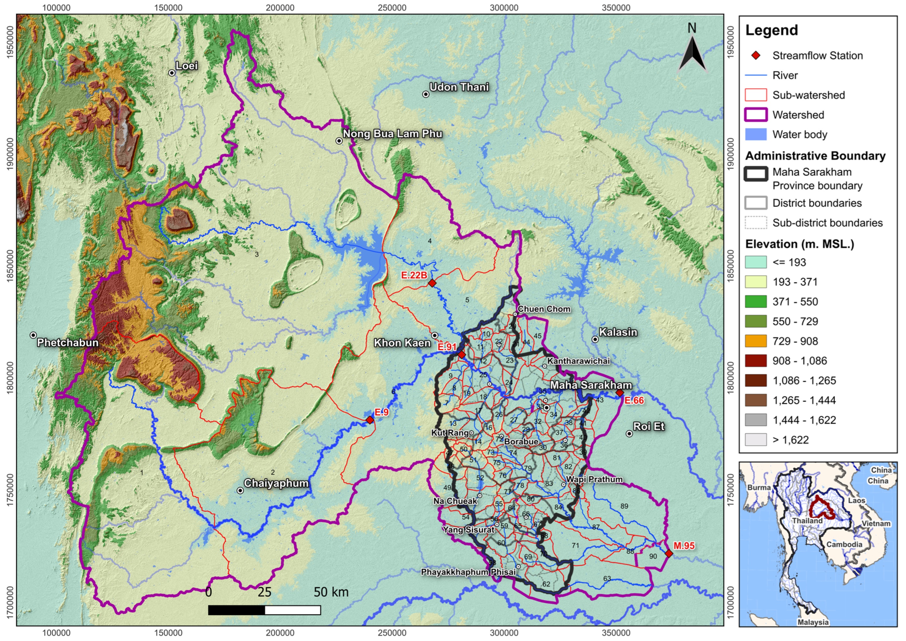
Figure 2.
Spatial distributions of meteorological monitoring stations and delineation of rainfall catchment areas using the Thiessen polygon method.
Figure 2.
Spatial distributions of meteorological monitoring stations and delineation of rainfall catchment areas using the Thiessen polygon method.
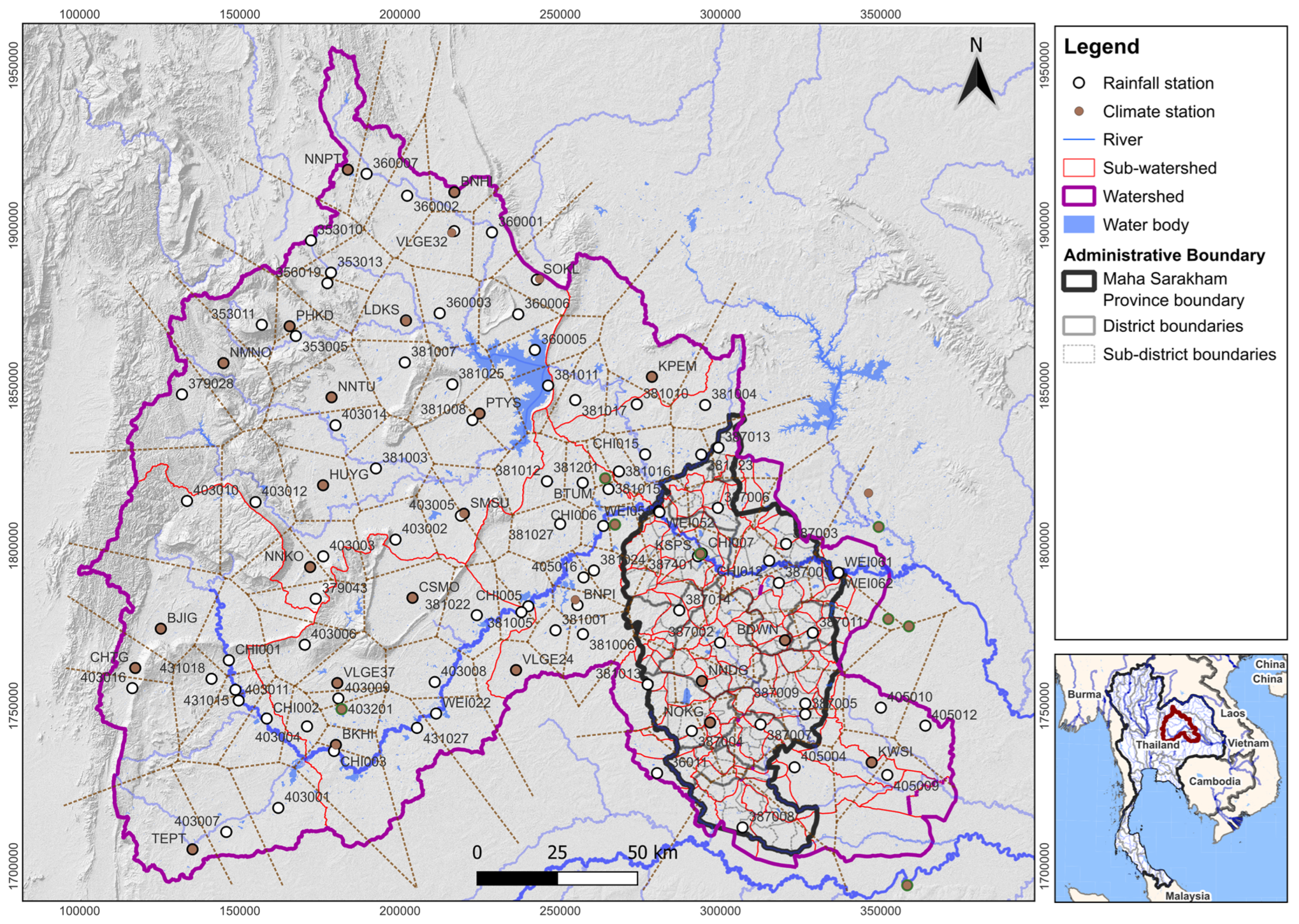
Figure 3.
Spatial data for the development of QSWAT HRUs: (a) Land use map; (b) Soil type map.
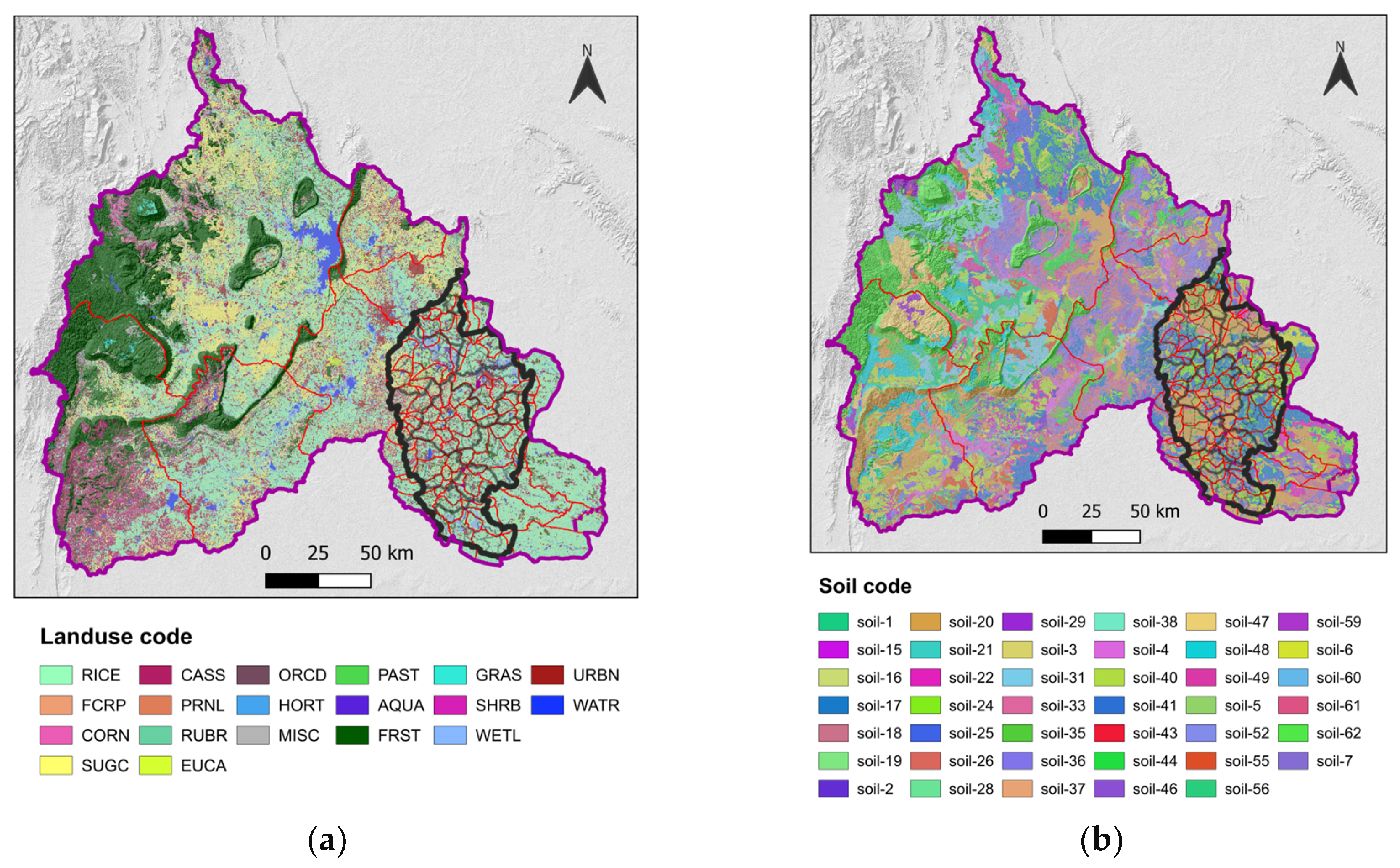
Figure 4.
Spatial data used for water balance assessment in the WEAP model.
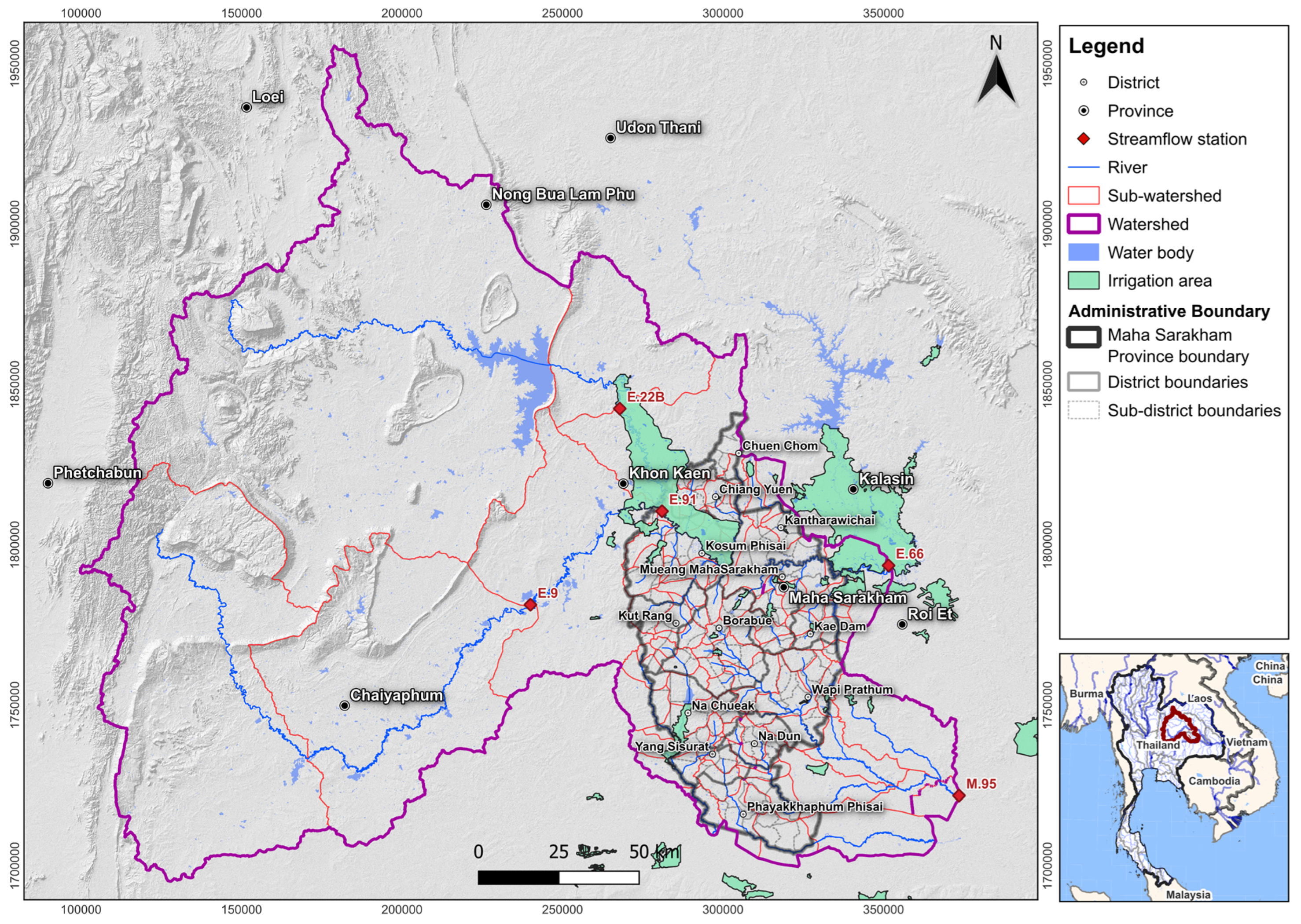
Figure 5.
Structure and components of the WEAP model in Maha Sarakham Province.
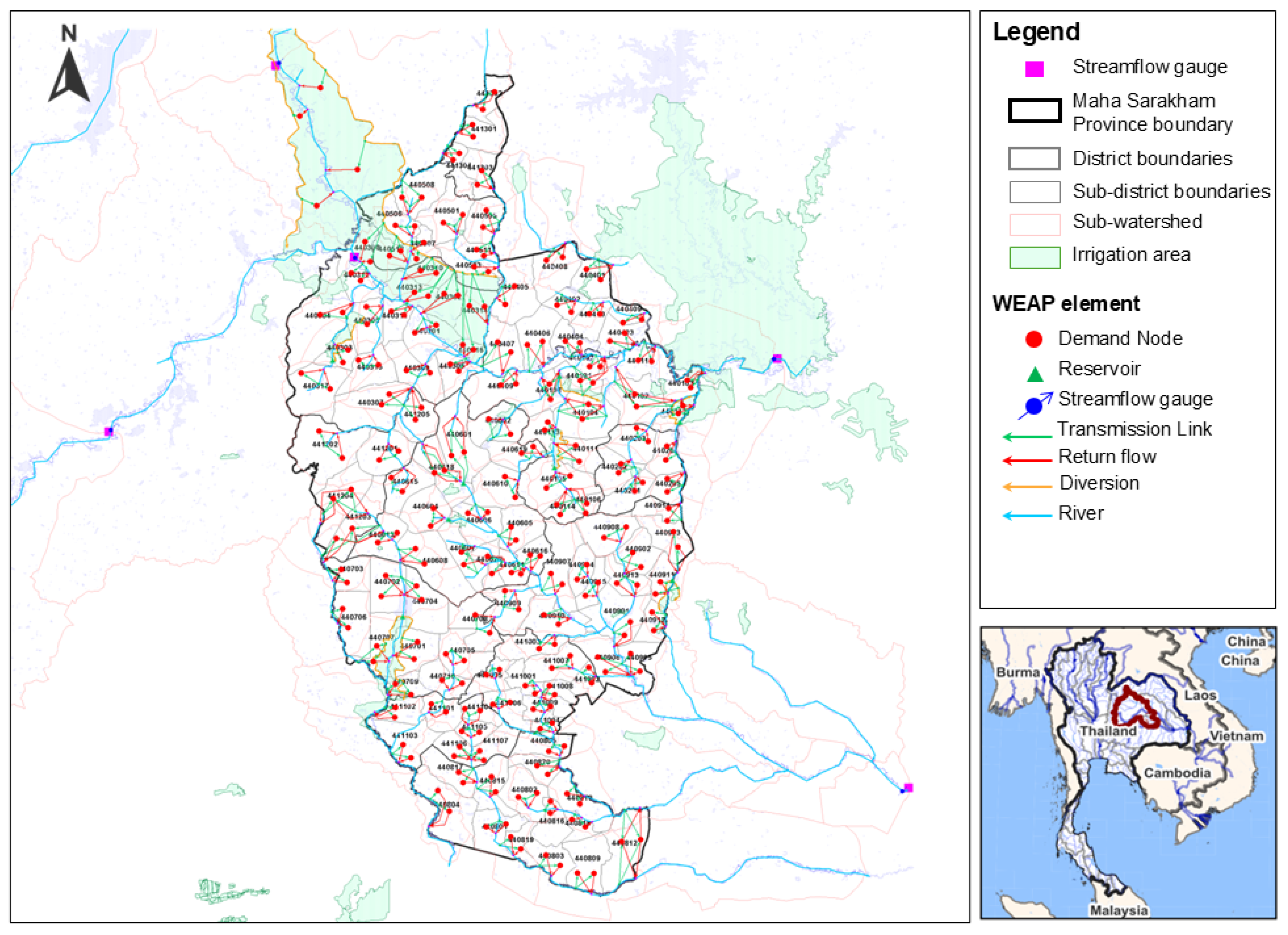
Figure 6.
Framework for water balance assessment using QSWAT-WEAP integration.
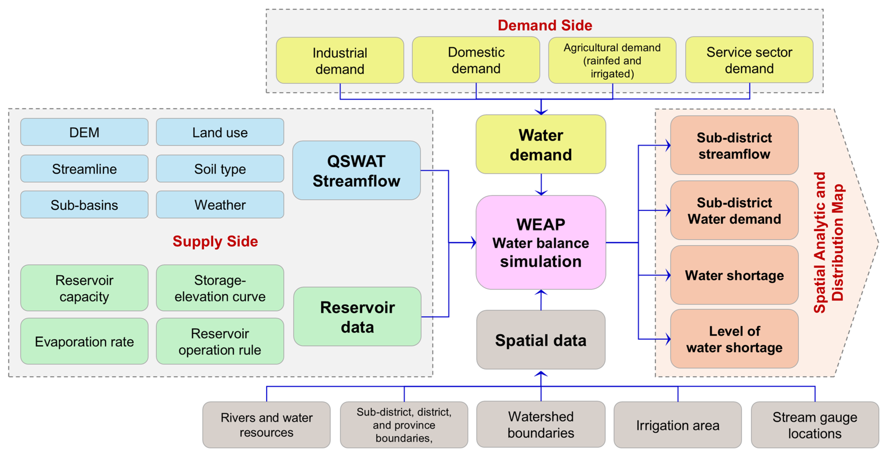
Figure 7.
QSWAT and WEAP performance assessment results.
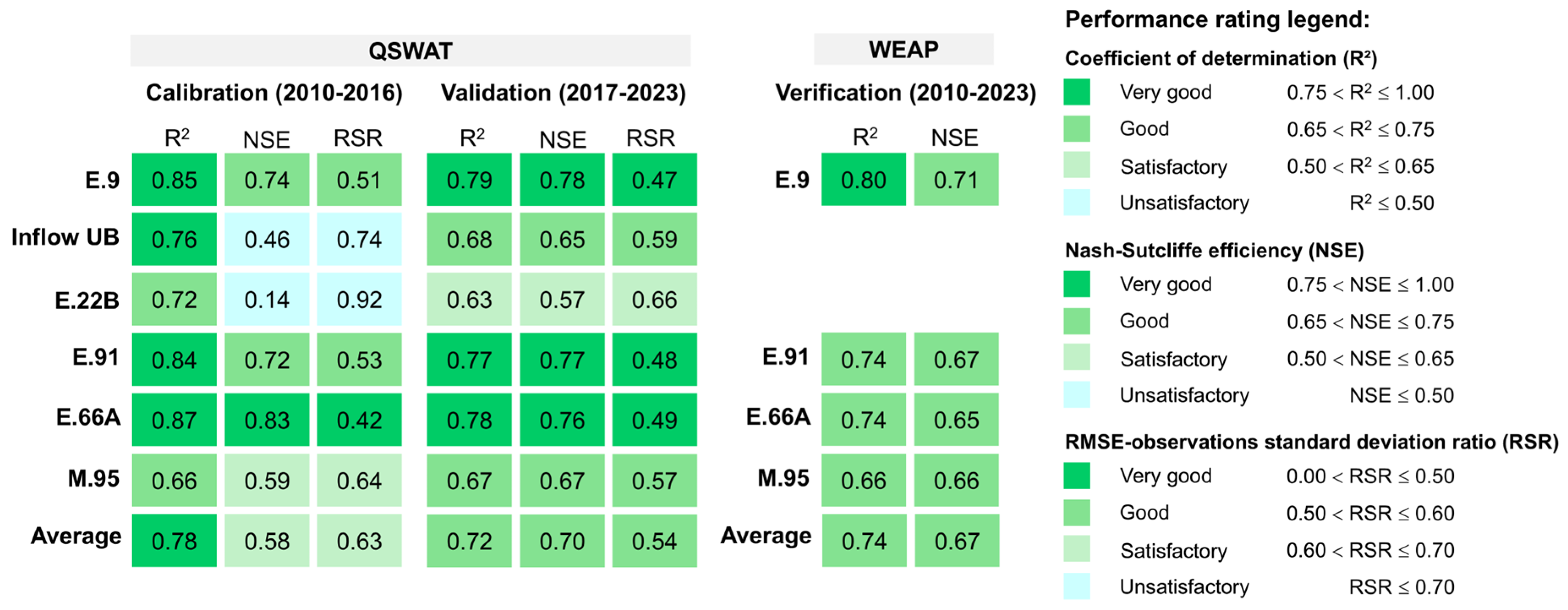
Figure 8.
Comparison of QSWAT and WEAP simulated streamflow with observed data (2010-2023): (a) E.9; (b) Inflow of Ubolrat Dam; (c) E.22B, (d) E.91; (e) E.66A; (f) M.95.
Figure 8.
Comparison of QSWAT and WEAP simulated streamflow with observed data (2010-2023): (a) E.9; (b) Inflow of Ubolrat Dam; (c) E.22B, (d) E.91; (e) E.66A; (f) M.95.
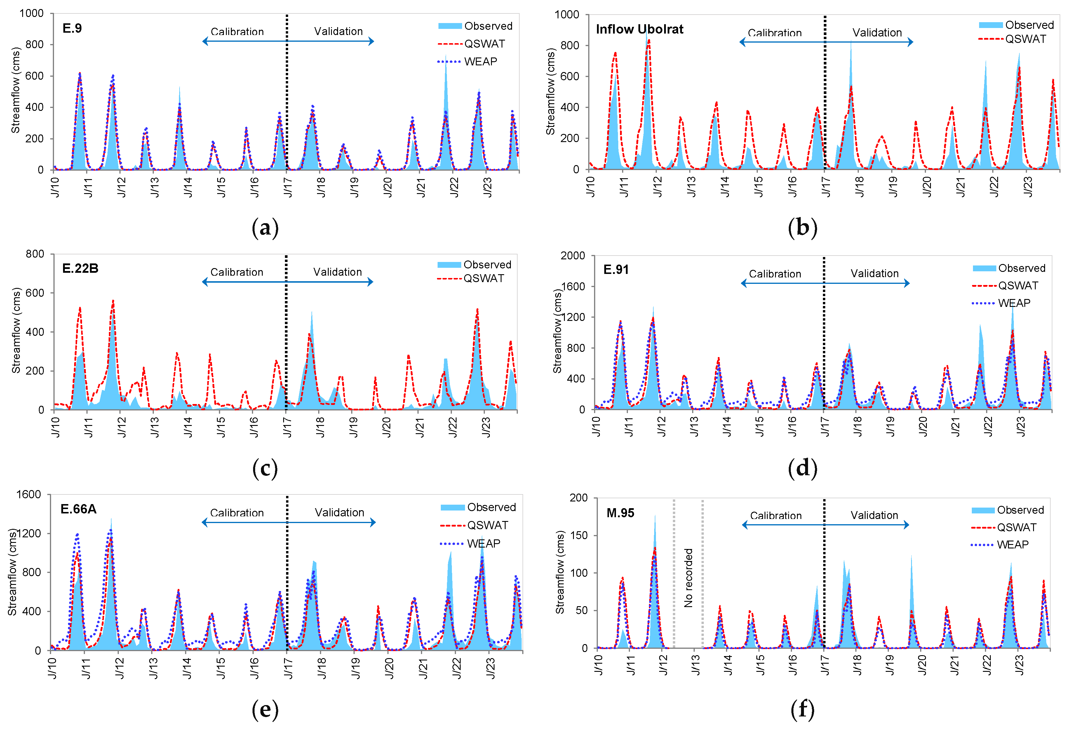
Figure 8.
Sub-district streamflow analysis: (a) spatial distribution by sub-district; (b) quantitative area analysis at the local level; (c) monthly temporal changes in Range 1-3; (d) monthly temporal changes in Ranges 4-5.
Figure 8.
Sub-district streamflow analysis: (a) spatial distribution by sub-district; (b) quantitative area analysis at the local level; (c) monthly temporal changes in Range 1-3; (d) monthly temporal changes in Ranges 4-5.
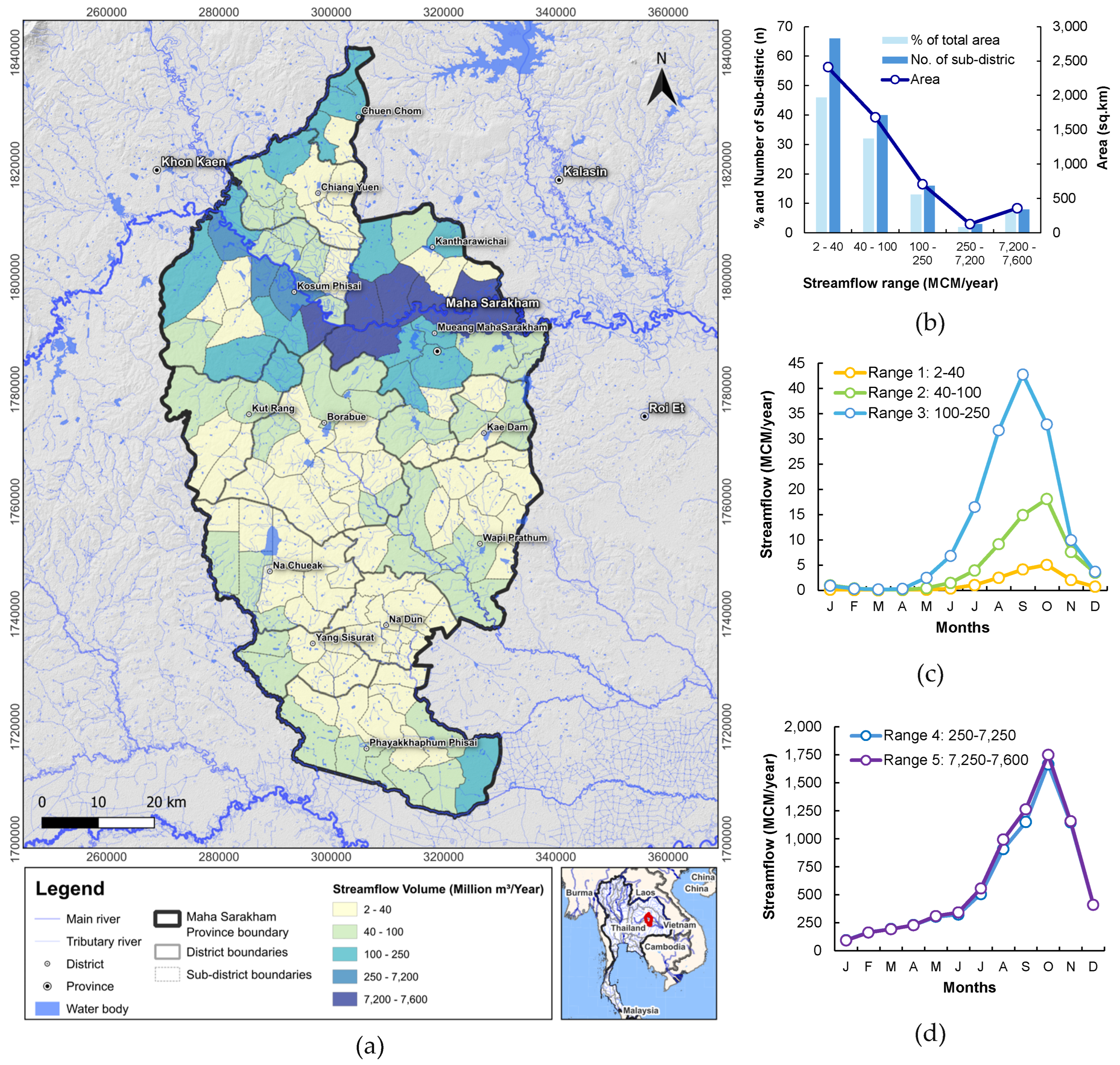
Figure 10.
Sub-district water demand analysis: (a) spatial distribution by sub-district; (b) quantitative area analysis at the local level; (c) monthly temporal changes in Ranges 1-5; (d) average annual water demand by sector; (e) annual quantity temporal changes.
Figure 10.
Sub-district water demand analysis: (a) spatial distribution by sub-district; (b) quantitative area analysis at the local level; (c) monthly temporal changes in Ranges 1-5; (d) average annual water demand by sector; (e) annual quantity temporal changes.
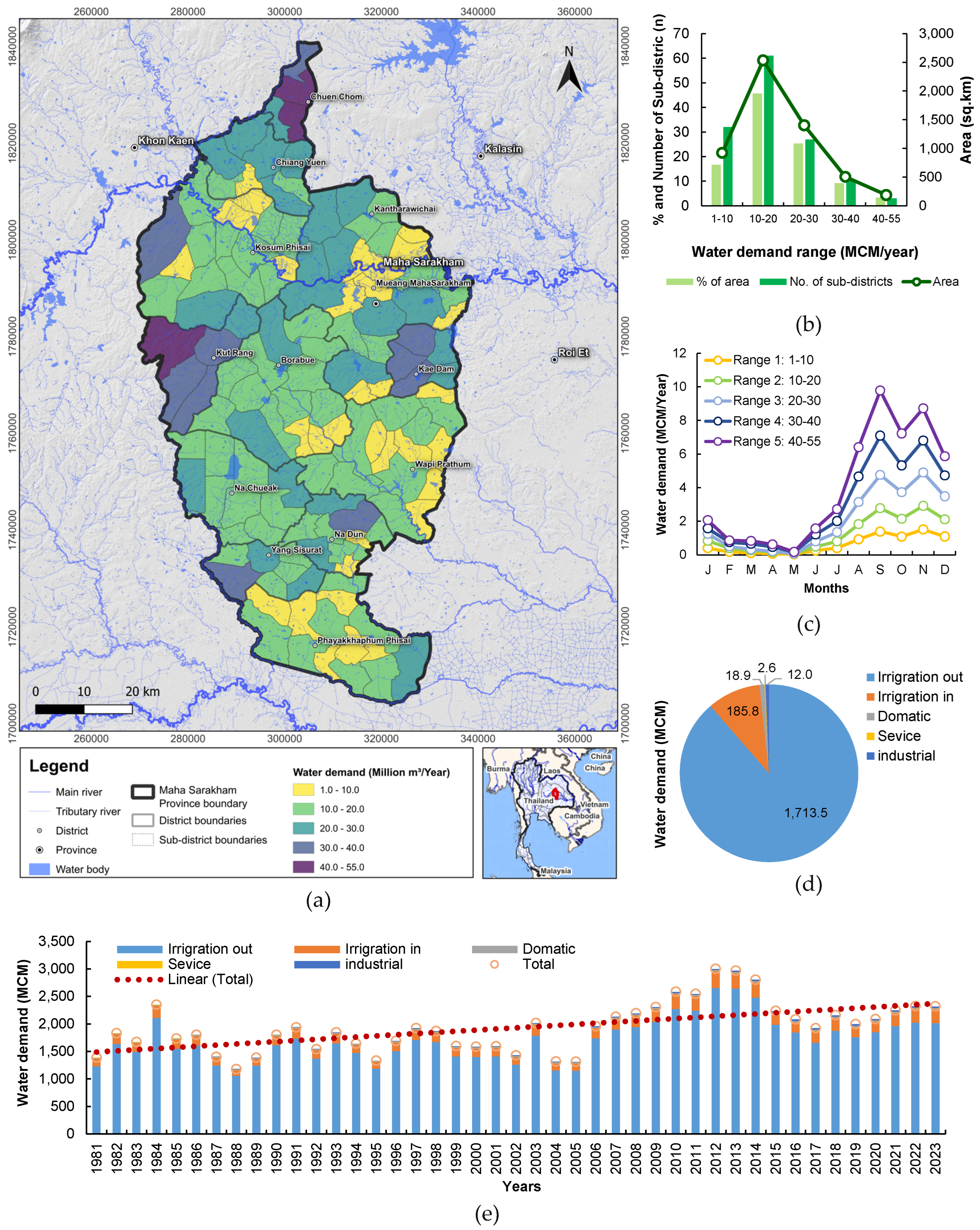
Figure 11.
Sub-district water shortage analysis: (a) spatial distribution by sub-district; (b) quantitative area analysis at the local level; (c) monthly temporal changes in Range 1; (d) monthly temporal changes in Ranges 2-5.
Figure 11.
Sub-district water shortage analysis: (a) spatial distribution by sub-district; (b) quantitative area analysis at the local level; (c) monthly temporal changes in Range 1; (d) monthly temporal changes in Ranges 2-5.
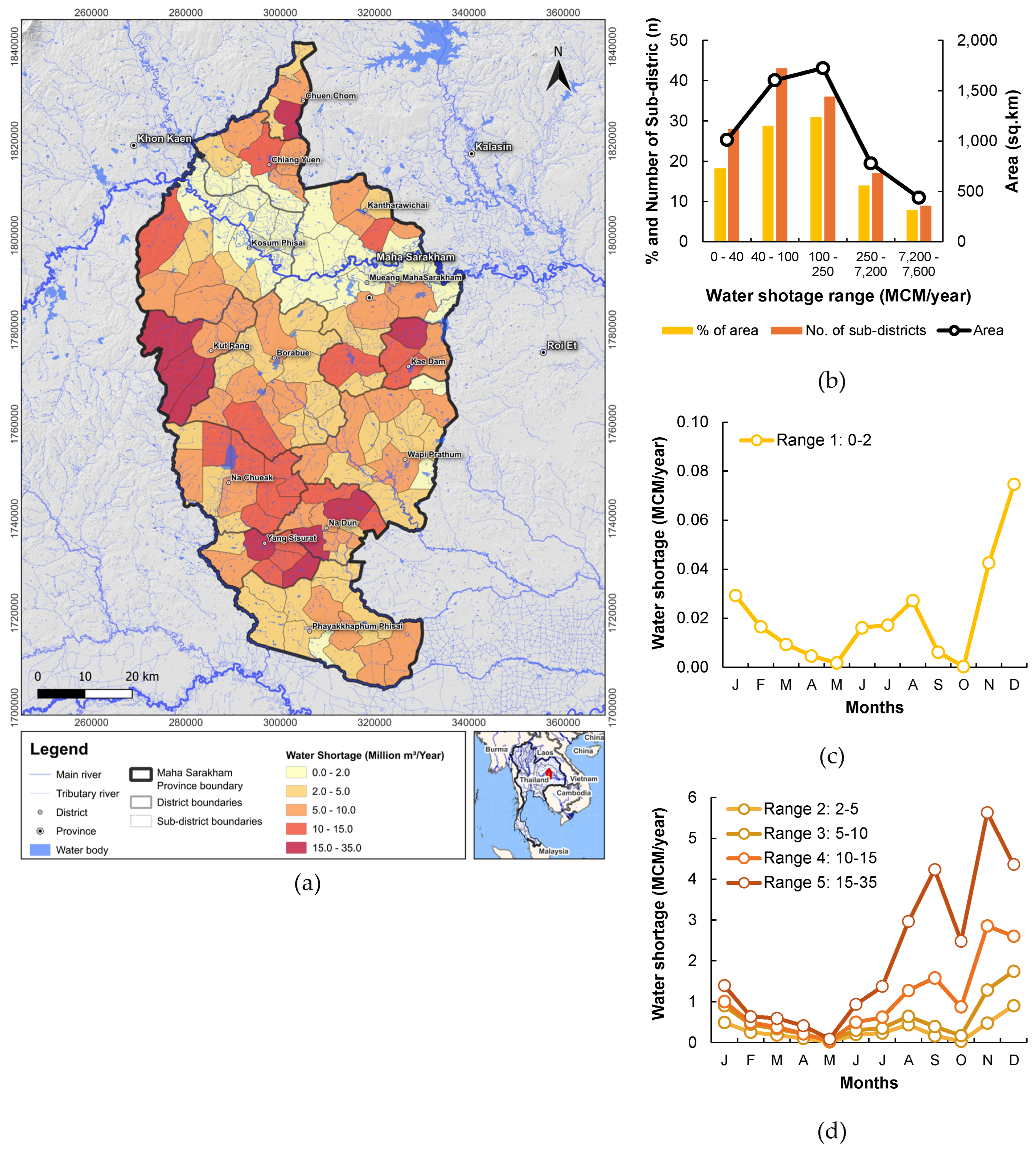
Figure 12.
Sub-district level of water shortage analysis: (a) spatial distribution by sub-district; (b) quantitative analysis at the local level from very low (0% - 5%) to very high (>45%); (c) monthly temporal changes in very low level (0% - 5%), and (d) monthly temporal changes in low level (5% - 15%) to very high (>45%).
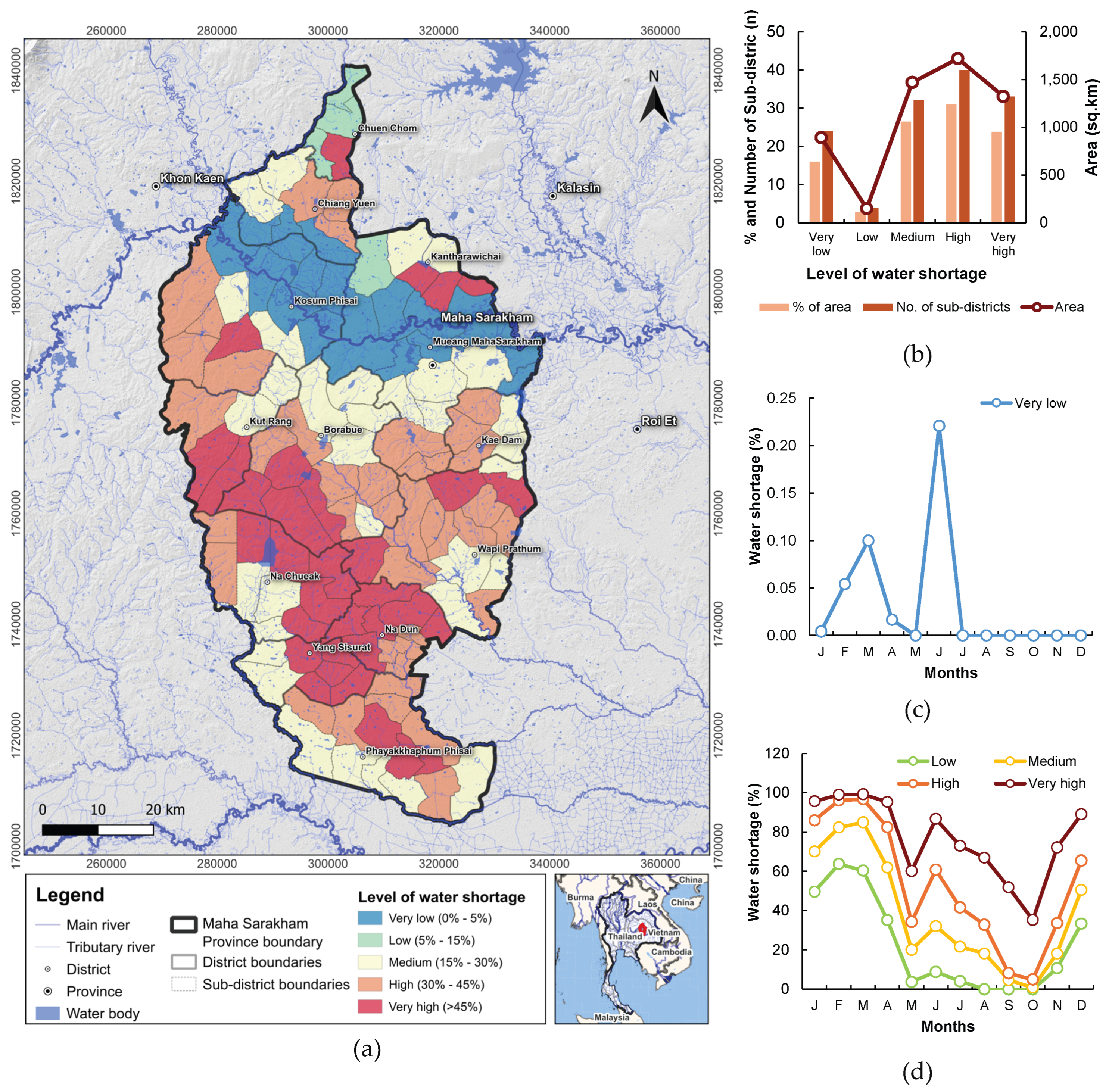

Table 1.
Data collection for QSWAT input.
| No. | Type of data | Resolution | Range | Sources |
|---|---|---|---|---|
| 1 | Watershed physical data | |||
| 1.1 | Digital Elevation Model (DEM) 30x30 m resolution | 30x30 m | 2019 | SRTM |
| 1.2 | Soil type map | 30x30 m | 2015 | LDD |
| 1.3 | Soil type map | 30x30 m | 2019 | LDD |
| 1.4 | Watershed boundary, water bodies, and stream network | DWR | ||
| 2 | Meteorological data | |||
| 2.1 | Rainfall | Daily | 2010 - 2023 | TMD, HII |
| 2.2 | Maximum-minimum temperatures, relative humidity, wind speed and sunshine hours |
Daily | 2010 - 2023 | TMD |
| 3 | Hydrological data | |||
| 3.1 | Streamflow at Stations E.9, E.22B, E.91, E.66A and M.95 | Daily | 2010 - 2023 | RID |
| 3.2 | Inflow of Ubolrat Reservoir | Daily | 2010 - 2023 | EGAT |
| 4 | Ubolrat Reservoir physical data | |||
| 4.1 | Normal and maximum storage capacity | Monthly | 2010 - 2023 | EGAT |
| 4.2 | Normal and maximum surface area | Monthly | 2010 - 2023 | EGAT |
| 4.3 | Storage target | Monthly | 2010 - 2023 | EGAT |
| 4.4 | Maximum-minimum release | Monthly | 2010 - 2023 | EGAT |
Table 2.
Data for WEAP input.
| No. | Type of Data | Remarks |
|---|---|---|
| 1 | Water supply data | Used for simulating streamflow and reservoir operation. |
| 1.1 | Streamflow data from the QSWAT model | |
| 1.2 | Reservoir data (reservoir capacity, storage-elevation curve, evaporation rate, reservoir operation rule) | |
| 2 | Spatial data | Used as background for creating river network and defining parameters in the WEAP model, as shown in Figure 4. |
| 2.1 | Rivers and water resources | |
| 2.2 | Sub-district, district, and province boundaries | |
| 2.3 | Watershed boundaries | |
| 2.4 | Irrigation area (within the study area, irrigated land covers 1,098.2 sq.km, of which Maha Sarakham Province accounts for 402.6 sq.km (36.8%)) | |
| 2.5 | Stream gauge locations | |
| 3 | Water demand data | Used for determining water demand in each sub-district. |
| 3.1 | Agricultural water demand (rainfed area and irrigated area) | |
| 3.2 | Domestic water demand | |
| 3.3 | Industrial water demand | |
| 3.4 | Service sector water demand |
Table 3.
The optimal parameter values obtained from calibration and validation of QSWAT.
| Rank | Parameter | Descriotion | Fitted Value | Adjust Range | t-Stat | p-Value |
|---|---|---|---|---|---|---|
| 1 | V__GWQMN.gw | Baseflow alpha factor (days) | 3537.500 | 0 - 5000 | 7.30 | 0.000000 |
| 2 | R__SOL_AWC(..).sol | Available water capacity of the soil layer | 0.07 | -0.4 - 0.4 | 5.64 | 0.000000 |
| 3 | V__GW_REVAP.gw | Groundwater “revap” coefficient | 0.18 | 0.02 - 0.2 | 5.31 | 0.000000 |
| 4 | V__ALPHA_BF.gw | Treshold depth of water in the shallow aquifer required for return flow to occur (mm) | 0.83 | 0 - 1 | 3.62 | 0.000381 |
| 5 | V__GW_DELAY.gw | Groundwater delay (days) | 362.85 | 30 - 450 | 2.36 | 0.019295 |
| 6 | R__SOL_K(..).sol | Saturated hydraulic conductivity | 0.05 | -0.4 - 0.4 | -1.89 | 0.060140 |
| 7 | R__CN2.mgt | SCS runoff curve number | 0.07 | -0.5 - 0.1 | 1.56 | 0.121035 |
| 8 | V__CH_N2.rte | Manning’s “n” value for the main channel | 0.02 | 0.01 - 0.1 | -1.48 | 0.140046 |
| 9 | V__CH_K2.rte | Effective hydraulic conductivity in main channel alluvium | 26.50 | 0 - 200 | -1.17 | 0.242679 |
| 10 | V__REVAPMN.gw | Threshold depth of water in the shallow aquifer for “revap” to occur (mm) | 48.750 | 0 - 100 | 0.84 | 0.399348 |
| 11 | V__EPCO.bsn | Plant uptake compensation factor | 0.94 | 0 - 1 | 0.70 | 0.482973 |
| 12 | V__CH_N1.sub | Manning’s “n” value for the tributary channels | 0.022 | 0.01 - 0.1 | -0.50 | 0.615715 |
| 13 | V__ESCO.bsn | Soil evaporation compensation factor | 0.868 | 0 - 1 | -0.47 | 0.639584 |
| 14 | R__SLSUBBSN.hru | Average slope length | -0.330 | -0.4 - 0.4 | 0.07 | 0.941914 |
Table 4.
Synthesis of water balance and shortage risk assessment by sub-district classification.
| Classification | No. of Sub-districts |
Area (sq.km) | % of total area |
Streamflow level (MCM per year) | Demand level (MCM per year) | Shortage level | Risk level |
|---|---|---|---|---|---|---|---|
| Surplus | 11 | 489 | 9 | High: Ranges 4-5 (250-7,600) | Low-Medium: Ranges 1-3 (1-30) | Very Low - Low | Low |
| Balanced | 16 | 709 | 13 | Medium: Range 3 (100-250) | Medium: Ranges 2-3 (10-30) |
Medium | Moderate |
| Deficit | 106 | 4,094 | 78 | Low: Ranges 1-2 (2-100) |
Medium-High: Ranges 2-5 (10-55) |
High - Very High | High |
| Total | 133 | 5,292 | 100 |
Table 5.
Characteristics of sub-districts by water shortage risk level.
| Risk level | No. of sub-districts |
Area (sq.km) | % of area | Distance from Chi River (km) | Streamflow density (MCM per sq.km) |
Primary water source | Critical period | Key vulnerability factor |
|---|---|---|---|---|---|---|---|---|
| Very low | 24 | 846 | 16.0 | < 5 | > 100 | Chi River | None | Low vulnerability |
| Low | 4 | 143 | 2.7 | 5 - 10 | 10 - 100 | Chi River + tributaries | Mar - Apr | Limited dry season supply |
| Medium | 32 | 1,397 | 26.4 | 10 - 15 | 2 - 10 | Tributaries | Feb - May | Seasonal fluctuation |
| High | 40 | 1,664 | 31.4 | 15 - 25 | 0.5 - 2 | Tributaries + rainfall | Jan - May | Distance from main river |
| Very high | 33 | 1,242 | 23.5 | > 25 | < 0.5 | Rainfall dependent |
Nov - Jun | No reliable water source |
| Total | 133 | 5,292 | 100 |
Disclaimer/Publisher’s Note: The statements, opinions and data contained in all publications are solely those of the individual author(s) and contributor(s) and not of MDPI and/or the editor(s). MDPI and/or the editor(s) disclaim responsibility for any injury to people or property resulting from any ideas, methods, instructions or products referred to in the content. |
© 2026 by the authors. Licensee MDPI, Basel, Switzerland. This article is an open access article distributed under the terms and conditions of the Creative Commons Attribution (CC BY) license (http://creativecommons.org/licenses/by/4.0/).
Copyright: This open access article is published under a Creative Commons CC BY 4.0 license, which permit the free download, distribution, and reuse, provided that the author and preprint are cited in any reuse.


