
Submitted:
10 January 2026
Posted:
12 January 2026
You are already at the latest version
Abstract
SLAM-based laser scanners generate extremely dense point clouds burdened with a high level of surface noise arising from random measurement errors and repeated scanning of identical regions. This increases data volume and complicates subsequent processing. The present study introduces four novel noise filtering and subsampling algorithms that selectively preserve the points closest to the true surface. Each algorithm assigns a filtering characteristic to individual points based either on their distance from a locally estimated (planar or quadratic) surface or on the degree of local eccentricity in the spherical neighborhood of the point. The proposed methods were tested on point clouds acquired using three SLAM scanners (Emesent Hovermap ST-X, FARO Orbis, and ZEB Horizon) in three different scenes with reference data acquired by a static terrestrial scanner Leica P40. All four proposed methods effectively reduced surface noise and data volume without compromising the cloud quality, clearly outperforming the standard subsampling tools (random, octree, or spatial subsampling). The most reliable surface noise removal in point clouds dominated by planar surfaces (building interior with planar walls) was achieved using the method based on local plane fitting. In contrast, the use of a quadratic surface proved more effective for uneven or rugged surfaces.
Keywords:
point cloud
; subsambling
; filtering
; SLAM
; 3D scanning
1. Introduction
Laser scanning systems, including static laser scanners (SLS), have become a well-established technology in many fields, including civil engineering, industry, and environmental sciences. In recent years, the use of handheld kinematic scanners based on Simultaneous Localization and Mapping (SLAM) algorithms is on the rise. These systems significantly accelerate data acquisition and can be employed in a wide range of environments [1,2,3,4,5].
Point clouds produced by SLAM scanners differ fundamentally from those acquired using static scanners in that the scanned surfaces have non-negligible thickness – in other words, the profile (i.e., cross-section) of the scanned surface is relatively thick compared to static scanners (see [6,7]). This results from two principal factors, namely the (typically) centimeter-level accuracy of the rangefinders and the repeated scanning of the same areas during motion. In practice, the resulting thickness of the point cloud may reach several centimeters, depending on the scanner type, and the point density within a profile follows a normal distribution. Consequently, a large number of redundant points are present, which complicates further processing both due to the sheer data volume and the fact that further processing steps typically assume a point cloud with negligible thickness (as is the case in point clouds acquired by static terrestrial scanners). The same issue (though less pronounced) can also be observed in point clouds acquired using 3D scanners mounted on unmanned aerial vehicles ([8,9]). For further processing, it is, therefore, highly desirable to dilute (subsample) the point cloud and to filter out as much noise as possible.
Numerous subsampling methods have been developed so far. They can generally be categorized into methods based on surface reconstruction using triangulated irregular networks (TIN), methods operating directly on the points within the dataset, and approaches employing machine learning techniques, such as neural networks. However, these approaches cannot be reasonably used on SLAM data due to the inherent “depth” (as mentioned above, these methods assume relatively thin point clouds) and the sheer amount of SLAM data, which leads to extreme computational demands.
For example, application of TIN-based methods ([9,10,11,12,13,14,15]) to noisy SLAM point clouds would result in the creation of an excessive number of randomly oriented triangles. Methods directly subsampling point clouds typically aim to achieve a spatial coverage of the scanned surface that is as uniform as possible, which is the case of algorithms such as Random Sampling (RS, [16]), Uniformly Voxelized Sampling (UVS, known also as octree subsampling [17]), Farthest Point Sampling (FPS, [18]), or Spatial Sampling (SS) used in CloudCompare software.
The Random sampling method simply selects points from the cloud at random until a predefined target quota is reached, either in terms of an absolute or relative (percentage of dilution) number of points. The UVS/octree method retains one point per voxel at a selected level of the octree structure, typically the point closest to the voxel center. Farthest Point Sampling iteratively selects points that are farthest from the already selected points, thus aiming to achieve the most faithful representation of the original point cloud for a given target number of points. In Spatial Sampling, a minimum distance between any two points is defined. The algorithm then selects points from the original cloud in a way to ensure that no point in the output cloud lies closer to another point than the specified threshold; increasing this value results in a lower number of retained points.
An interesting approach to subsampling aims to reduce the number of points in the cloud progressively by retaining fewer points in simple areas and more points in geometrically complex regions, thus preserving the quality of the surface representation as much as possible while greatly reducing the point cloud size [19]. Yet another approach to point reduction relies on the detection of key points [20,21,22,23,24], sufficient to describe the scanned object. Such key points are typically located at the corners and edges, i.e., points located at the margin of the cloud. Noisy SLAM point clouds, however, pose a fundamental challenge for these methods, as the points at the margin of the cloud are inherently the most distant from the true surface, thus constituting the least reliable points in the cloud.
Other algorithms are based on deep learning or artificial intelligence [25,26,27]. However, similarly to TIN-based methods, their practical applicability for real-world point clouds is limited by high computational demands.
The issue of cloud denoising is closely related to subsampling. The use of deep neural networks in the field of denoising has been rapidly evolving over the last few years. However, the regularity of the input data is a common prerequisite for applying neural networks to point cloud processing. This typically requires transforming the point cloud into a voxel-based representation, as employed, for example, in the MSVC terrain filtering method [28]. This limitation is partially addressed in the PointNet neural network architecture [29], which directly processes the entire irregular point cloud and segments it into meaningful objects. Other tools build upon this network and combine its advantages with additional approaches to noise filtering [30,31]. However, the datasets used for training and testing in these studies are synthetic and contain significantly fewer points than real-world point clouds. The reason for this lies in the computational demands of these algorithms: every point in the point cloud is represented by at least three parameters (coordinates; the use of additional parameters, such as intensity or color, further increases the demands), and a sufficiently large neighborhood of each point must be applied to enable its classification. A common SLAM-acquired cloud comprises 200 mil. points, leading to a large number of points even in a relatively small neighborhood (for example, approx. 4,000 points are likely to fall within a spherical neighborhood with a radius of 50 mm). In view of the computational demands for calculating such an immense task, the use of neural networks for real-world SLAM data would be too computationally demanding.
To complete the list, it is also necessary to mention statistical filters for the identification and filtering of outliers, such as the SOR filter (Statistical Outlier Removal, PCL library [32]). This filter is, however, designed for the removal of outliers, but not for the removal of the Gaussian noise produced by SLAM scanners. Smoothing methods can, of course, also be used to reduce noise; they, however, do not dilute the cloud but only move the points closer to the fitted surface (e.g. [33]). In this way, a principally new point cloud is created, consisting largely of points that are not real but rather conform to the adopted approximation, while the original points are lost.
All the above implies that the current widely used subsampling/noise filtering methods are suboptimal for subsampling and noise filtering of dense SLAM-acquired point clouds, and that other approaches respecting the characteristics of such clouds are needed for this purpose.
Here, we propose a new approach through four algorithms performing simultaneous subsampling and noise filtering of SLAM-acquired point clouds. These algorithms are designed to preferentially remove points distant from the scanned surface, thus, at the same time, reducing excessive data volume. This paper, therefore, aims: (i) to define new methods for simultaneous subsampling of SLAM-acquired clouds and surface noise filtering, (ii) to test these methods and their parameters on real-world datasets, including comparisons with commonly used approaches, with high-accuracy point clouds serving as a reference, and (iii) to identify the most effective algorithm out of the newly proposed ones.
2. Materials and Methods
2.1. Tested Methods
The surface noise in SLAM-acquired point clouds is approximately normally distributed; the most likely position of correct points is, therefore, in the region of the highest density of the points (if considering the direction perpendicular to the actual surface). A comparison of a terrestrial scanner, Leica P40 with extremely low noise, and a SLAM scanner is shown in Figure 1).
Four methods to subsampling combined with filtering of the surface noise will be proposed and tested here. All these methods are based on the estimate of the true position of the scanned surface, followed by a calculation of a characteristic of the quality of each point compared to the estimated surface. In the last step, the points are sorted according to the value of this characteristic (thus forming a histogram of points with the horizontal axis indicating their quality), and a selected percentage of the points with the poorest values is removed. In two of the proposed methods, the scanned surface is simulated using a planar surface within a spherical neighborhood of each point, while a quadratic surface is fitted in the other two methods. The four methods are:
- Standardized distance to the planar surface (SDP),
- Ratio of standard deviations from the planar surfaces (RSDP),
- Standardized distance to quadratic surface (SDQ),
- Ratio of standard deviations relative to quadratic surfaces (RSDQ).
The common first step for all four algorithms lies in the identification of all points within a spherical neighborhood of each respective point. The radius of the spherical neighborhood should be greater than the maximum noise distance from the surface (“maximum noise thickness” in the entire cloud) to allow reasonable fitting of the surface approximation (see Figure 2).
2.1.1. Standardized Distance to the Planar Surface (SDP)
This method uses a plane passing through the center of gravity of all points within the spherical neighborhood, which is defined by the coordinates of the center of gravity and by the normal vector. Once this plane (center of gravity plane) is fitted by the least squares method, the closest (perpendicular) distance of each evaluated point from the plane is calculated (Figure 2) and divided by the standard deviation of the plane fit (in this case, standard deviation from the center of gravity plane, SDCGP) as follows (Equations (1,2,3)):
where d stands for distance of the i-th point from the plane, A, B, C, D are plane coefficients, x, y, z are the i-th point coordinates, n is the number of points within the spherical neighborhood, and PI indicates the point of interest.
The SDP value, therefore, shows the distance of the point from the plane expressed in multiples of standard deviation. This calculation is performed for (and the SDP value assigned to) each point within the point cloud.
2.1.2. Ratio of Standard Deviations from the Planar Surface (RSDP)
Within each spherical neighborhood, the standard deviation of distances of all points from the plane fitted to pass through the center of gravity (i.e., the plane used in the SDP method) is always the lowest possible (i.e., lower than the standard deviation relative to any other plane passing through the spherical neighborhood). A second plane is also fitted to all points in the spherical neighborhood, but this plane is forced to pass through the investigated point. Subsequently, the standard deviation of all points from the second plane (investigated point plane, SDIPP) is also calculated. RSDB is then acquired as a ratio of the two variances (i.e., SD2) following Equation (4):
Each point then acquires its RSDP characteristic, ranging from 0 to 1. The further the respective point is from the center of gravity plane, the poorer is the fit of the investigated point plane and the higher is its standard deviation, resulting in a lower RSDP value (Figure 3).
2.1.3. Standardized Distance to the Quadratic Surface (SDQ)
If a curved surface is being scanned, the linear approximation used in the two previous “planar” methods can be insufficient for satisfactory noise filtering. For this reason, quadratic surface approximation might be more suitable for real-world applications (Figure 4a,b). However, the full equation describing a general quadratic surface contains a large number of parameters, which makes its use computationally demanding. This can, fortunately, be avoided through simplification of the surface orientation. First, an auxiliary plane is fitted to all points in the spherical neighborhood of the investigated point and the entire neighborhood is spatially transformed (rotated about axes x, y, and z) so that the normal vector of this auxiliary plane is parallel to the z axis. This provides mathematical simplification of subsequent operations while also ensuring that the mutual relationships (distances) between points in the spherical neighborhood remain unchanged. Such a quadratic surface can then be described by Equation (5):
where A, B, C, D, E, and F are coefficients of the quadratic surface, x, y, z are the coordinates of points resting on the quadratic surface.
After this transformation, a quadratic surface best fitting all points in the transformed spherical neighborhood is calculated using the least squares method. The z-differences (Δz) are calculated from Equation (6) and the standard deviation of the z-differences is calculated from Equation (7). The resulting SDQ parameter is then calculated using Equation (8).
where n is the number of points within the spherical neighborhood and PI is the point of interest.
2.1.4. Ratio of Standard Deviations Relative to Quadratic Surfaces (RSDQ)
This method is equivalent to the RSDP method; the difference lies only in the use of a quadratic surface instead of a planar one. The first quadratic surface is fitted to all points in the spherical neighborhood, the second is also fitted to all points but forced to pass through the point of interest (Figure 5). The RSDQ parameter is then calculated as the ratio of variances of all points in the neighborhood relative to each of the quadratic surfaces (9).
where σF2 is the variance of the best-fitting quadratic surface, and σPI2 is the variance of the quadratic surface forced to pass through the point of interest.
2.2. Evaluation of the Proposed Methods
The proposed methods were used to assign metrics to each point in the cloud. As an example, Figure 6 shows a part of the point cloud with individual colors indicating the values of the SDQ metric.
The performance of each of the methods is then expected to depend on two parameters, namely the radius of the spherical neighborhood and the cut-off percentile used to remove points based on the values of the given metric (SDP, RSDP, SDQ, RSDQ). For this reason, it was crucial to evaluate the RMSDs of subsampled point clouds (relative to the reference cloud) resulting from multiple combinations of spherical neighborhood radius (0.0125 m, 0.025 m, 0.05 m, 0.1 m, and 0.2 m) and cut-off values (removing points with a step of 10%, i.e., 10% of the points with the highest values of the metric, 20%... 90% were removed). In addition, the distances between points in the resulting subsampled clouds and their RMSDs were evaluated.
The RMSDs relative to the reference surface (constructed using triangular irregular network from 15 closest points in the reference cloud acquired using a highly accurate terrestrial scanner Leica P40, with an accuracy of 1 mm) were calculated in CloudCompare for the remaining points (cloud-to-cloud distance function) and these RMSDs, calculated according to the Equation (10), were compared among methods and cut-off parameters.
where di is the distance of the i-th point from the retained cloud from the reference surface, and n is the number of all points in the retained cloud.
To be able to properly evaluate the performance of the proposed methods, their RMSD values were subsequently compared mutually and with commonly used subsampling methods, namely octree subsampling (in each voxel of a given octree level, a single point closest to the voxel center was preserved), random subsampling (a given percentage of points were randomly removed) and spatial subsampling (based on the minimum allowed distance between points). The parameters used for subsampling by the standard methods are detailed in Table 1.
2.3. Testing Point Clouds
As SLAM scanners are typically used for scanning indoor environments, and as it would be impossible to properly evaluate the accuracy of the resulting filtered clouds in an outdoor environment (due to the typical fine motion of vegetation, preventing the determination of an accurate reference cloud), two indoor scenes were used for evaluation.
The first scene (Hallway) captures a part of a building including a vertical pipe but generally dominated by planar surfaces (Figure 7a). To be able to more accurately evaluate the effect of filtering approaches on the edges, a corner part of that point cloud was evaluated separately (Hallway detail) (Figure 7b). To include a highly complex surface, a tunnel with highly rugged surface was added (Tunnel, Figure 7c). In view of the static character of the reference terrestrial scanner Leica P40, parts of the clouds were not available in the reference cloud due to shadowing effects and were removed from the evaluated clouds to allow reasonable comparison of the clouds (these parts are white in Figure 10).
Each scene was scanned, besides the aforementioned reference scanner Leica P40, with three SLAM scanners, namely Emesent Hovermap ST-X (Emesent, Australia), FARO Orbis (FARO Inc., USA), and Geoslam ZEB Horizon (Geoslam, United Kingdom). The parameters of individual point clouds are detailed in Table 2.
It is necessary to keep in mind that point clouds acquired using SLAM scanners are necessarily slightly distorted due to the principle of their scanning. For this reason (and because in this paper, we do not evaluate the performance of individual scanners but the performance of individual noise filtering/subsampling methods), the point clouds acquired using SLAM scanners were transformed to the reference cloud using the ICP (iterative closest point) algorithm. This ensured the best possible fit of the individual clouds to the reference cloud, thus leading to the elimination of systematic errors between the cloud points that could otherwise influence the results of accuracy of the filtered/subsampled clouds.
3. Results
3.1. Evaluation of the Best Neighborhood for Each Method
For each scanner-scene combination, the relationship between the resulting RMSD (relative to the reference cloud) and the percentile cut-off value calculated for each tested value of the spherical neighborhood and for each of the tested methods was plotted. One example of such a plot is depicted in Figure 8 (all plots are shown in the Appendix A, Figure A1, Figure A2, Figure A3). The spherical neighborhood showing the best RMSDs across the entire range of cut-off values (i.e., the lowest area under the curve, AUC) was then always chosen as the best-performing neighborhood and used for subsequent evaluations. The resulting best neighborhoods for individual scene/scanner/method combinations, along with RMSDs of the original clouds, are presented in Table 3. The accuracy of newer scanners (Emesent Hovermap ST-X, FARO Orbis) is substantially better (RMSDs of 5-6 mm) than that of the older SLAM scanner ZEB Horizon (10-13 mm). A general trend of larger spherical neighborhoods being more suitable for quadratic methods and for less accurate scanners can be observed. Still, it is necessary to select a spherical neighborhood of sufficient radius to contain the entire profile captured by the scanner – this is clearly demonstrated by the poor performance of the smallest tested radius of 0.0125 m in Figure 8. On the other hand, if the spherical neighborhood is too large (0.1, 0.2 m), the quadratic surface is unable to approximate sharp edges with sufficient accuracy, which reduces the quality of the filtering and produces rounded edges, see. Figure 9).
3.2. Challenging Aspects
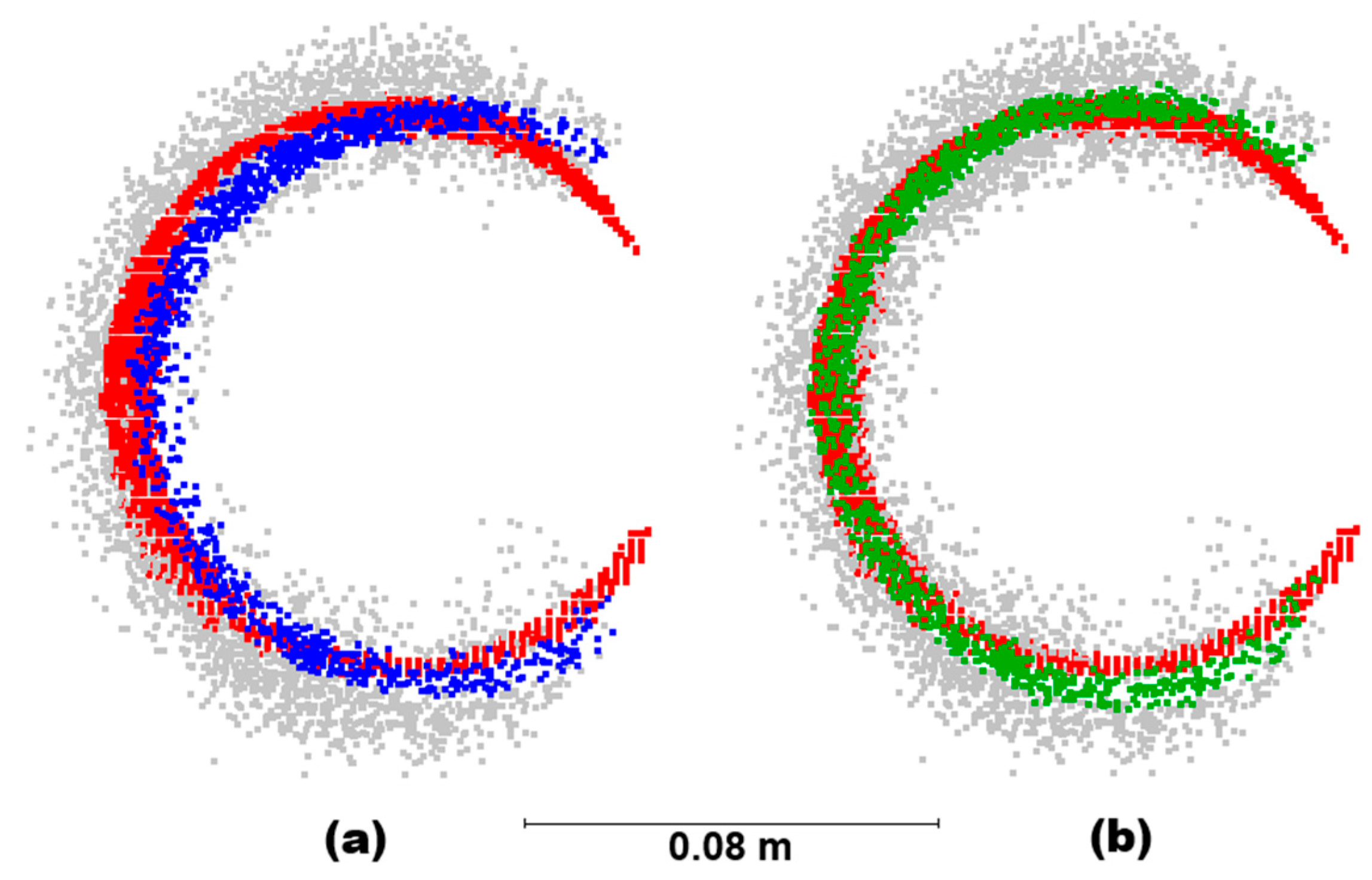
The waste piping at the wall in the Hallway scene offers a good illustration of the differences in the use of planar and quadratic methods on non-planar surfaces. As seen in Figure 10 (reference points are highlighted in red), the planar method (SDP, blue) incorrectly preserves the innermost points of the surface, removing most of the correct points, while the quadratic method (SDQ, green) is much more successful in identifying the actual surface.
Figure 10.
A profile of the detail of the Hallway scene containing piping. Red points indicate the reference cloud, grey points indicate the removed noise points. (a) Blue points show the result of filtering using SDP, while (b) green points present the result of SDQ filtering (both methods with 30% of preserved points, spherical neighborhood of 0.05 m, scanned with Emesent Hovermap ST-X). Note the better fit of the SDQ method to the reference cloud compared to the SDP method. The points of the filtered cloud are always in the foreground.
It is also necessary to consider an additional issue of residual outliers – when using the optimal radius of the spherical neighborhood, noise points that are further from the true surface than the radius itself remain preserved in the cloud (see Figure 11). This is caused by the fact that a lack of a reasonable number of points in the spherical neighborhood of the point representing noise can influence the fitting of the planar or quadratic surfaces, which then pass through the particular point and, as a result, the investigated point appears to have a low metric value; in effect, such points remain unfiltered (Figure 11b). This problem has been partially resolved by establishing a minimum number of six neighboring points, i.e., points with less than six other points in their spherical neighborhood were removed from the cloud. This method is helpful, but perfect removal of these residual outliers needs application of additional filtering (such as SOR, [32]), which will be the subject of further study.
3.3. The Influence of the Proportion of Preserved Points on the Accuracy
For practical use, as well as for the evaluation of the method's performance, establishing the correct level of filtering is crucial. Even though RMSDs generally improve with a greater proportion of removed points, a minimum required density/level of detail must be considered when setting up the cut-off. It is, therefore, not possible to establish a universal cut-off value. Figure 12 compares the original cloud (Figure 12a,b) with a cloud from which 90% of the points were filtered out (Figure 12c). The profiles obviate that despite such extensive filtering, the shape and geometric structure of the scene are preserved, which demonstrates the excellent performance of the method in removing redundant and erroneous points while preserving the points of highest quality.
Figure 13 plots the increasing mean distances between points during progressive filtering (the numbers are shown in Appendix B, Table A1). Considering the average accuracy of the new-generation SLAM scanners of approx. 2.5 cm (noise thickness), even the approx. 13 mm distance at the highest used level of filtering (90%) is still sufficient. However, one must keep in mind that the curves only show the distances between points; for this reason, Figure 13b was used for the visualization of one of the scenes (Hallway) along with the indicator of accuracy (RMSD). Note also that the distances between points after a 90% filtering depend on the original cloud density, which is influenced by multiple factors (scanner type, speed of motion during acquisition, distance, etc.), so this result needs to be interpreted with caution.
3.4. Performance of the Novel Filtering/Subsampling Methods
For each scene-scanner pair, results of all seven tested methods (with the best-performing spherical neighborhood in the case of the newly proposed methods) were plotted (see Figure 14 as an example; all plots are shown in the Appendix C, Figure A4, Figure A5, Figure A6). It is obvious that all four novel subsampling/filtering methods proposed in this paper lead to notable improvement of RMSD with increasing level of filtering. This is the opposite of the results of standard subsampling methods, in which RMSDs remain unchanged or deteriorate. For this reason, and to allow a clearer depiction, plots presented below will only compare the performances of the four novel methods.
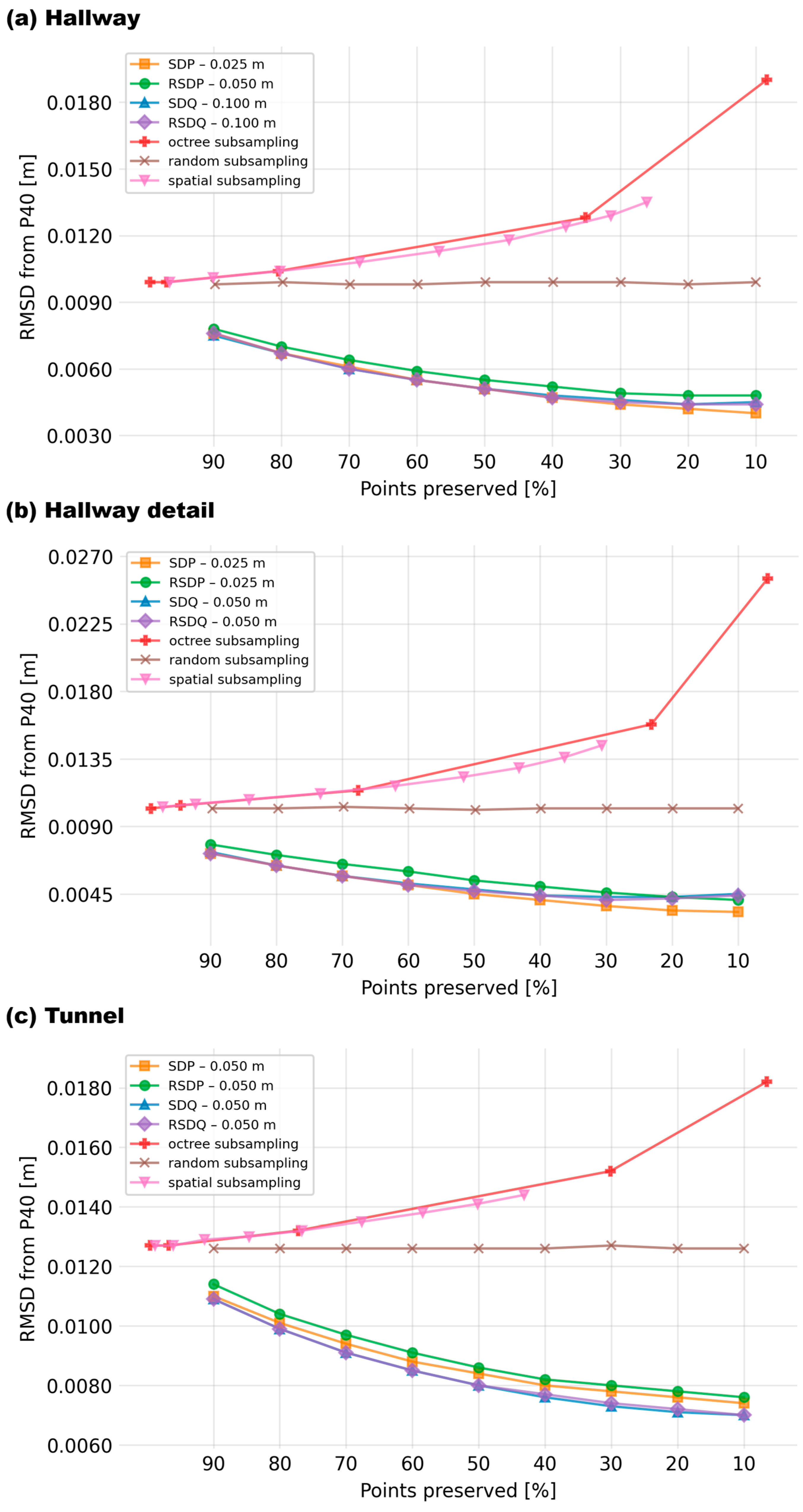
Figure 15 presents the comparison of the four developed algorithms across all scenes, scanners, and levels of filtering. All algorithms obviously greatly improved the accuracy, improving (after subsampling to 10% of the original cloud) the RMSDs by 50% or more compared to the original cloud in all instances, with the exception of ZEB Horizon in the Tunnel scene, where the improvement was only by 44%, see Appendix D, Table A2.
In the point clouds of scenes dominated by planar surfaces (Hallway and Hallway detail) acquired using the new generation scanners (Emesent Hovermap ST-X and FARO Orbis, Figure 15a,b,d,e, all methods performed similarly from the perspective of overall RMSD until the level of filtering of approx. 30%. Although the edges are likely better captured by the quadratic methods as demonstrated in Figure 10, there are too few of them in these two scenes to have a major impact on the overall RMSD. Still, the RSDP method appears to have the poorest performance in all these combinations, which is even more pronounced in the case of the less accurate ZEB Horizon (Figure 15g,h). In the case of the highly rugged surface of the tunnel (Figure 15c,f,i), quadratic methods (SDQ, RSDQ) clearly outperform the planar ones.
Interestingly, in certain scene-scanner combinations (Figure 15d,e,g,h), a deterioration in the performance of quadratic filters can be observed at very high dilution below 30%. This is caused by the residual outliers discussed above (Figure 11, Chapter 3.2). With the decreasing total number of points, the relative influence of these outliers increases, which leads to the growing RMSD at extreme dilutions. This effect was not observed in the case of the Tunnel scene due to the different character of the scene and the resulting clouds.
4. Discussion
The use of SLAM scanners has been growing in popularity over the last decade due to the ease of use and rapid scanning. However, SLAM-acquired point clouds, although very dense, suffer from a relatively high level of surface noise that reduces their accuracy. Standard subsampling/filtering methods are capable of diluting the point clouds to manageable numbers of points, but do not improve the reliability of the cloud. In this paper, we have proposed and tested four subsampling methods that not only reduce the number of points in the cloud, but, even more importantly, preferentially remove the lower quality points (i.e., noise).
All the proposed algorithms use a spherical neighborhood of each individual point for determining its quality. The radius of the spherical neighborhood is an important parameter influencing the performance of all proposed algorithms. Although no universally valid best-performing radius can be recommended based on our results, we can propose some general recommendations. Importantly, the radius must be sufficiently large to contain the entire noise profile; in effect, its size depends on the scanner and its accuracy. As a rule of thumb, we could propose a 2.5*rangefinder accuracy for the planar algorithms (SDP and RSDP) and 5*rangefinder accuracy for the algorithms using quadratic surfaces (SDQ and RSDQ). The higher values needed for the methods employing quadratic surfaces are caused by the curvature that needs to be taken into account for better performance of these algorithms. Note that this rule of thumb is valid for the initial estimation of the spherical neighborhood, but it needs to be fine-tuned based on a particular cloud and the evaluation of its noise. Still, as shown in Figure 8 (and Figure A1, Figure A2, Figure A3 in the Appendix A), the performance of the algorithms is relatively robust providing that the entire depth of the noise profile is captured (for example, in Figure 8, the results of radiuses of 0.025, 0.05, and 0.1 are pretty similar) and it is better to err on the side of caution by choosing a greater spherical neighborhood than a smaller one.
All four algorithms proposed in this study outperformed the standard subsampling algorithms (Figure 14). While these preserve the original accuracy of the cloud (random subsampling) or even worsen the original accuracy due to preferentially removing points from the densest, i.e., the most accurate, points within the cloud (octree, spatial subsampling), all the proposed algorithms actually lead to an improvement of accuracy with increasing level of subsampling because they preferentially remove the points that are furthest from the densest part of the cloud.
The mutual comparison of the proposed algorithms (Figure 15) then shows that the RSDP algorithm generally performs the worst of the lot (despite still significantly outperforming the standardly used algorithms). For simple planar surfaces (such as building interiors), the other planar algorithm (SDP) performs excellently until very high dilutions (dilution to 10% of the original cloud). On the other hand, quadratic approaches (SDQ, RSDQ) outperform it in the case of rugged uneven surfaces. It needs to be said that quadratic approaches perform well even for planar surfaces as long as the dilution is not to less than 30% of the original cloud and as such, they could be recommended as universally preferred if the required dilution does not exceed this level (not the least because the quadratic approaches better preserve the edges and corners even in clouds showing largely planar environments, such as building interiors; this better performance at the edges is, however, overwhelmed by the very high number of the points describing the planar surfaces).
The (albeit minor) decrease in the accuracy in planar environments at very high dilutions (below 30%) is the only downside of the quadratic approaches. This is largely caused by the aforementioned residual outliers, the relative amount of which increases with decreasing number of points in the cloud. Further research, which would likely comprise a combination of these algorithms with another method for outlier removal, needs to address this issue. Providing such a workflow is devised, it is highly likely that the quadratic approaches would perform much better even at high dilutions.
Comparison with the literature is difficult. The widely used subsampling methods discussed above are generally employed without giving thought to their unsuitability for SLAM data, and research on improving the quality of the cloud simultaneously with subsampling is almost non-existent in scientific literature. We are aware only of a single study addressing this issue [34]. In their paper, they divided the cloud into voxels and within each voxel, points were filtered based on the distances from a Poisson surface fitted to all points within the voxel. The authors have, however, not tested the results against an independent reference cloud. Testing was performed only on artificially introduced synthetic noise and the effect of their filtering on cloud accuracy was not quantified. The method employed in their paper allows only two parameters to be set – the level of octree (implying the voxel size) and the cut-off value for the multiple of standard deviation for preserving/removing points from the cloud. From this perspective, the simple selection of the percentage of points to be preserved can be considered a practical advantage of our approach.
From the perspective of computational demands, the quadratic approaches are more demanding than the planar ones, and the approaches using ratios (RSDP, RSDQ) are more demanding than those using only a single surface. Still, even with the most demanding algorithm (RSDQ), the filtering of the point cloud with approx. 2.5 mil. points took no more than a few minutes. Considering that the proposed approaches are capable of reducing real-world point clouds by up to 90%, while at the same time improving cloud accuracies by (typically) 50-70%, we believe that these approaches hold great promise for use in conjunction with SLAM scanners.
Limitations of the proposed algorithms include the aforementioned issue of outliers and slight rounding of edges (especially with the planar approaches). Also, the relatively longer time needed for the computation of quadratic approaches could be considered a limitation. However, these issues can be resolved by further research – for example, by creating a smart combined algorithm that would switch between the quadratic and planar methods depending on the region of the cloud.
5. Conclusions
To summarize the results, all four novel algorithms for simultaneous subsampling/noise filtering proposed in this paper outperformed the standard subsampling algorithms in terms of improving point cloud quality (improving the RMSD of the original cloud by approx. 50-70% with dilution to 30%-10% of the original cloud size). Planar algorithms (SDP, RSDP) performed very well on clouds from simple environments, such as building interiors with predominance of planar surfaces. Quadratic approaches can, however, be considered more universal, and when subsampling to no less than 30% of the original cloud, they could be considered preferable due to their greater versatility. Both quadratic approaches perform similarly; from this perspective, the SDQ could be recommended thanks to its lower computational demands.
Author Contributions
Conceptualization, M.B. and M.Š.; methodology, M.B. and M.Š.; software, M.B.; validation, M.B., M.Š. and H.V.; formal analysis, M.B. and M.Š.; investigation, M.B.; resources, M.B.; data curation, M.B.; writing—original draft preparation, M.B., M.Š. and H.V.; writing—review and editing, M.B., M.Š., H.V. and J.K.; visualization, H.V. and J.K.; supervision, M.Š.; project administration, M.B.; funding acquisition, M.B. All authors have read and agreed to the published version of the manuscript.
Funding
The research was co-funded by the Grant Agency of the Czech Technical University in Prague, grant No. SGS25/045/OHK1/1T/11 "Point cloud filtering and classification using machine learning methods" and The Technology Agency of The Czech Republic under the project MESVYVED no. SQ01010105.
Institutional Review Board Statement
Not applicable.
Informed Consent Statement
Not applicable.
Data Availability Statement
The data presented in this study are available on request from the corresponding author. The data are not publicly available due to the size of the data.
Conflicts of Interest
The authors declare no conflicts of interest.
Appendix A
Figure A1.
Plots of RMSDs of Emesent Hovermap ST-X scans relative to the reference cloud resulting from individual filtering cut-offs (preserving 90% to 10% of the points) for individual sizes (radii) of the spherical neighborhood. Each row shows results for different method (SDP – (a-c), RSDP – (d-f), SDQ – (g-i), RSDQ – (j-l)), each column shows results for a different scene (Hallway – (a,d,g,j); Hallway detail – (b,e,h,k); Tunnel – (c,f,i,l)).
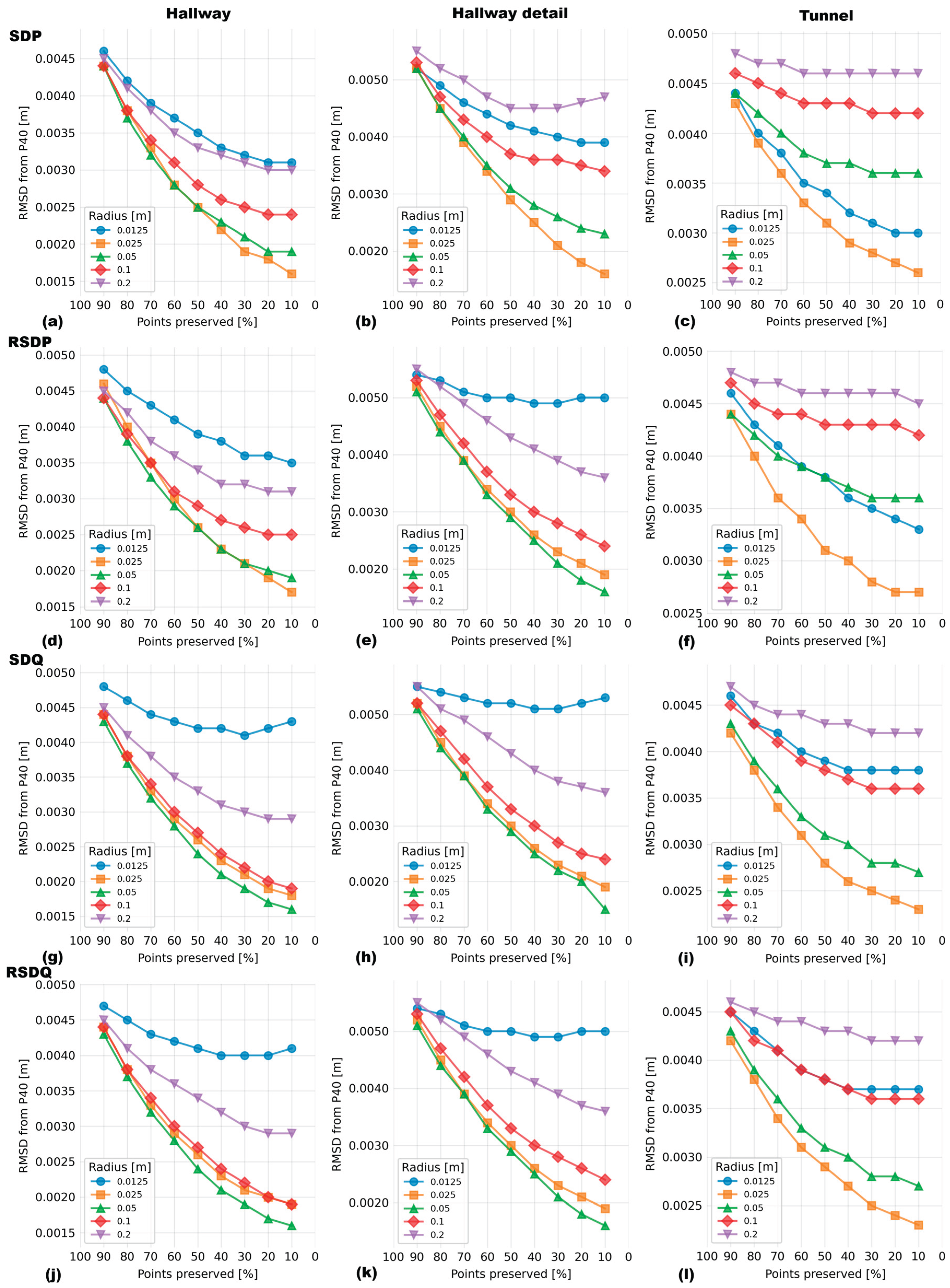
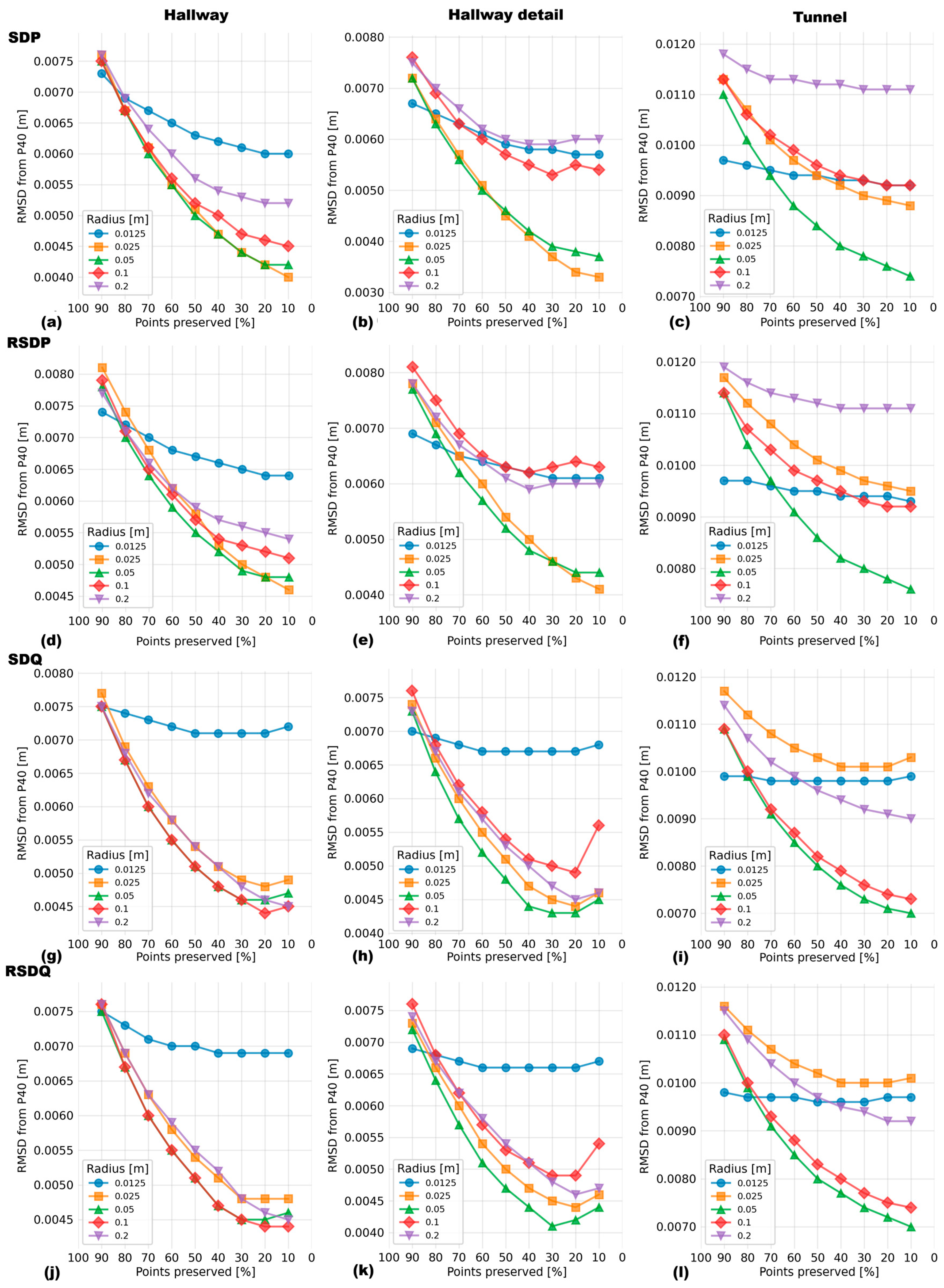
Figure A2.
Plots of RMSDs of FARO Orbis scans relative to the reference cloud resulting from individual filtering cut-offs (preserving 90% to 10% of the points) for individual sizes (radii) of the spherical neighborhood. Each row shows results for different method (SDP – (a-c), RSDP – (d-f), SDQ – (g-i), RSDQ – (j-l)), each column shows results for a different scene (Hallway – (a,d,g,j); Hallway detail – (b,e,h,k); Tunnel – (c,f,i,l)).
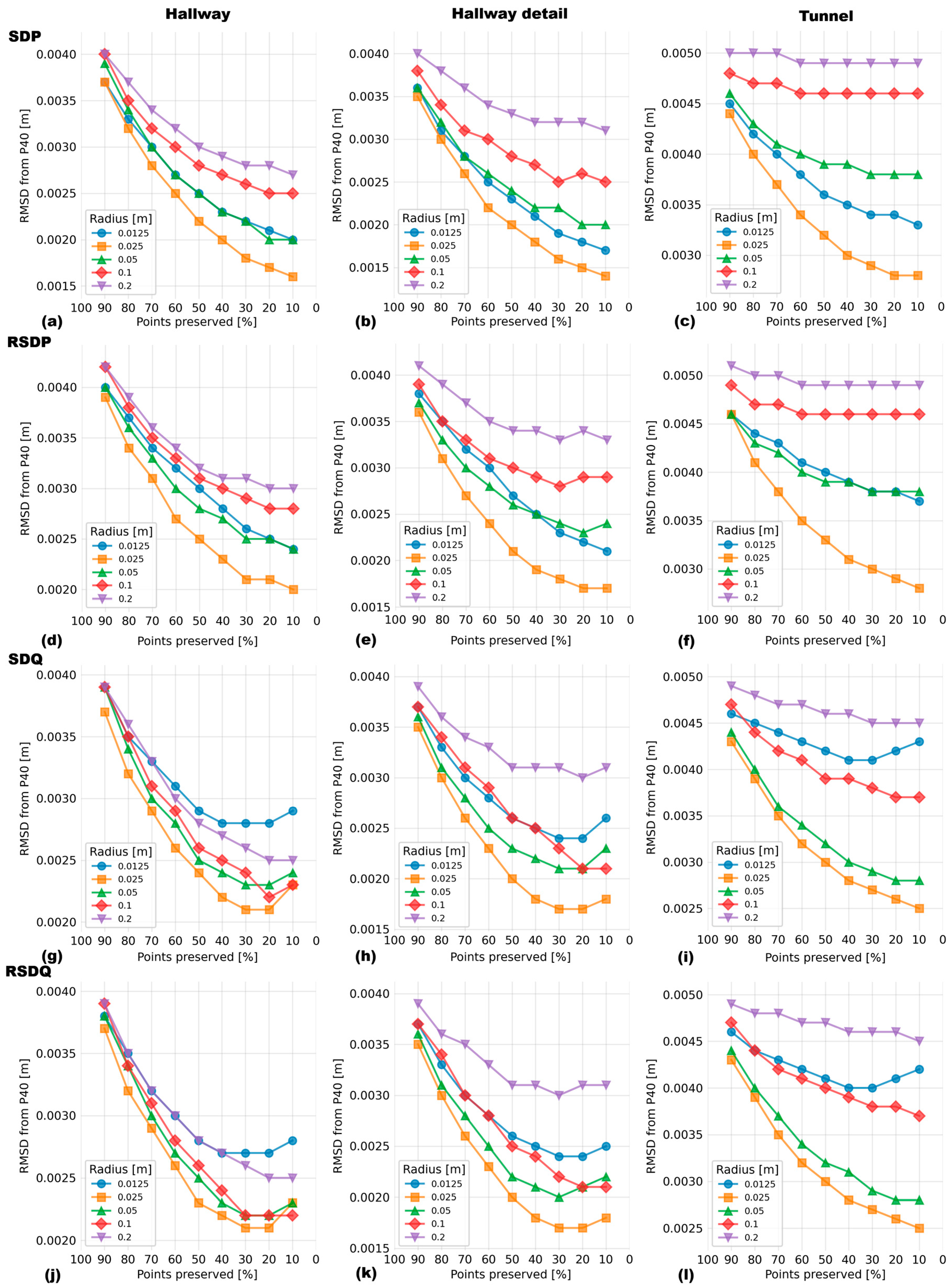
Figure A3.
Plots of RMSDs of ZEB Horizon scans relative to the reference cloud resulting from individual filtering cut-offs (preserving 90% to 10% of the points) for individual sizes (radii) of the spherical neighborhood. Each row shows results for different method (SDP – (a-c), RSDP – (d-f), SDQ – (g-i), RSDQ – (j-l)), each column shows results for a different scene (Hallway – (a,d,g,j); Hallway detail – (b,e,h,k); Tunnel – (c,f,i,l)).
Appendix B

Table A1.
Mean point-to-point distance [m] of neighboring points at gradual filtering – SDQ, with a spherical neighborhood with radius of 0.05 m.
Table A1.
Mean point-to-point distance [m] of neighboring points at gradual filtering – SDQ, with a spherical neighborhood with radius of 0.05 m.
| Scanner | Scene | Points preserved [%] | |||||||||
|---|---|---|---|---|---|---|---|---|---|---|---|
| 100 | 90 | 80 | 70 | 60 | 50 | 40 | 30 | 20 | 10 | ||
| Emesent Hovermap ST-X | Hallway | 0.004 | 0.005 | 0.005 | 0.005 | 0.006 | 0.006 | 0.007 | 0.008 | 0.010 | 0.014 |
| Hallway detail | 0.005 | 0.005 | 0.005 | 0.006 | 0.006 | 0.007 | 0.007 | 0.008 | 0.010 | 0.014 | |
| Tunnel | 0.004 | 0.004 | 0.004 | 0.005 | 0.005 | 0.005 | 0.006 | 0.007 | 0.008 | 0.012 | |
| FARO Orbis | Hallway | 0.003 | 0.003 | 0.003 | 0.004 | 0.004 | 0.004 | 0.005 | 0.006 | 0.007 | 0.010 |
| Hallway detail | 0.003 | 0.003 | 0.003 | 0.004 | 0.004 | 0.004 | 0.005 | 0.005 | 0.007 | 0.009 | |
| Tunnel | 0.004 | 0.004 | 0.005 | 0.005 | 0.005 | 0.006 | 0.007 | 0.008 | 0.009 | 0.013 | |
| ZEB Horizon | Hallway | 0.004 | 0.004 | 0.005 | 0.005 | 0.005 | 0.006 | 0.006 | 0.007 | 0.009 | 0.013 |
| Hallway detail | 0.005 | 0.005 | 0.005 | 0.006 | 0.006 | 0.007 | 0.007 | 0.009 | 0.010 | 0.015 | |
| Tunnel | 0.006 | 0.006 | 0.006 | 0.007 | 0.007 | 0.008 | 0.009 | 0.010 | 0.012 | 0.017 | |
Appendix C
Figure A4.
RMSDs acquired after different degrees of filtering with standard filtering/subsampling approaches and with the novel approach introduced in this study scanned with Emesent Hovermap ST-X in different scenes – (a) Hallway, (b) Hallway detail, (c) Tunnel.
Figure A4.
RMSDs acquired after different degrees of filtering with standard filtering/subsampling approaches and with the novel approach introduced in this study scanned with Emesent Hovermap ST-X in different scenes – (a) Hallway, (b) Hallway detail, (c) Tunnel.
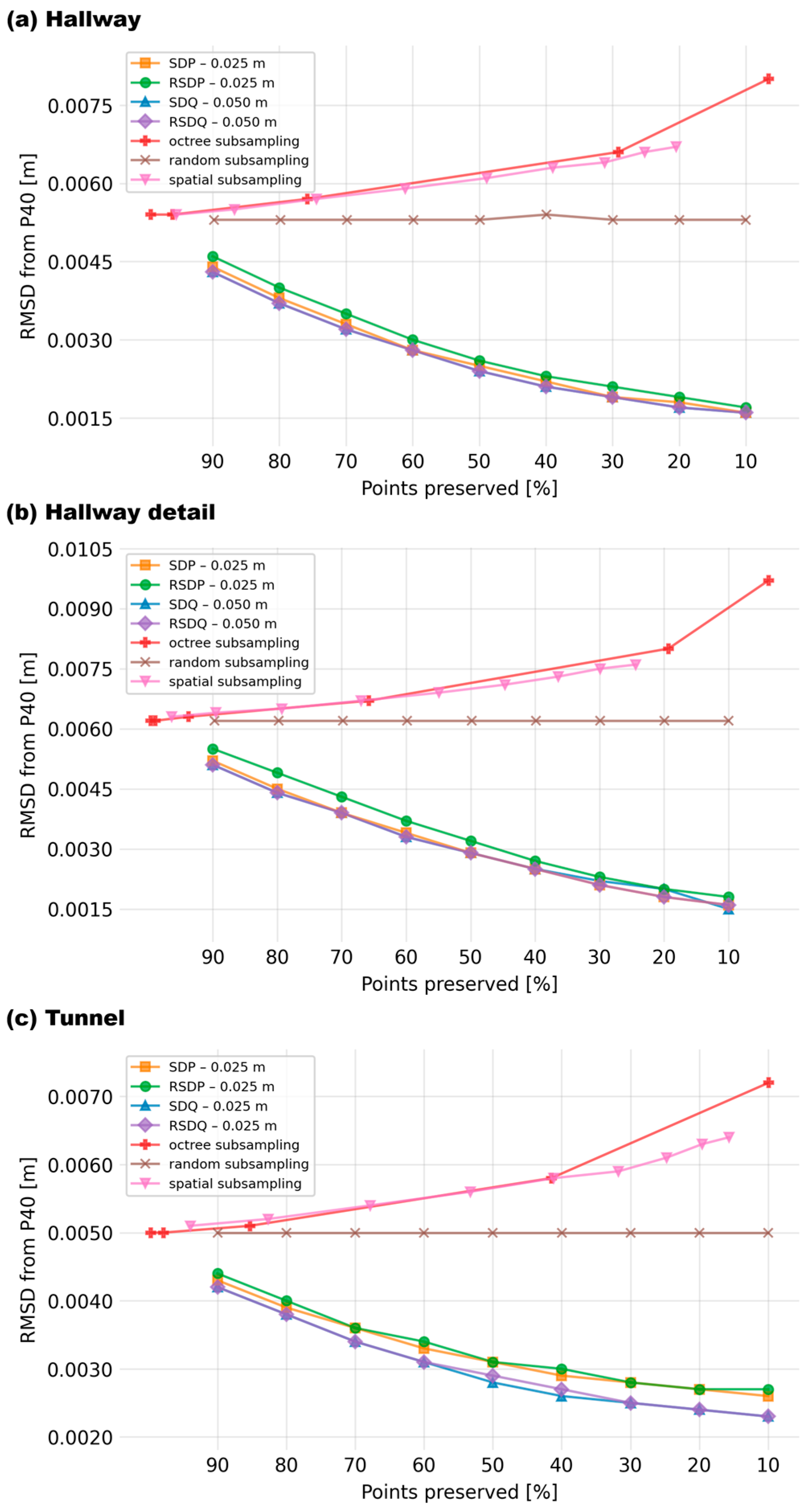
Figure A5.
RMSDs acquired after different degrees of filtering with standard filtering/subsampling approaches and with the novel approach introduced in this study scanned with FARO Orbis in different scenes – (a) Hallway, (b) Hallway detail, (c) Tunnel.
Figure A5.
RMSDs acquired after different degrees of filtering with standard filtering/subsampling approaches and with the novel approach introduced in this study scanned with FARO Orbis in different scenes – (a) Hallway, (b) Hallway detail, (c) Tunnel.
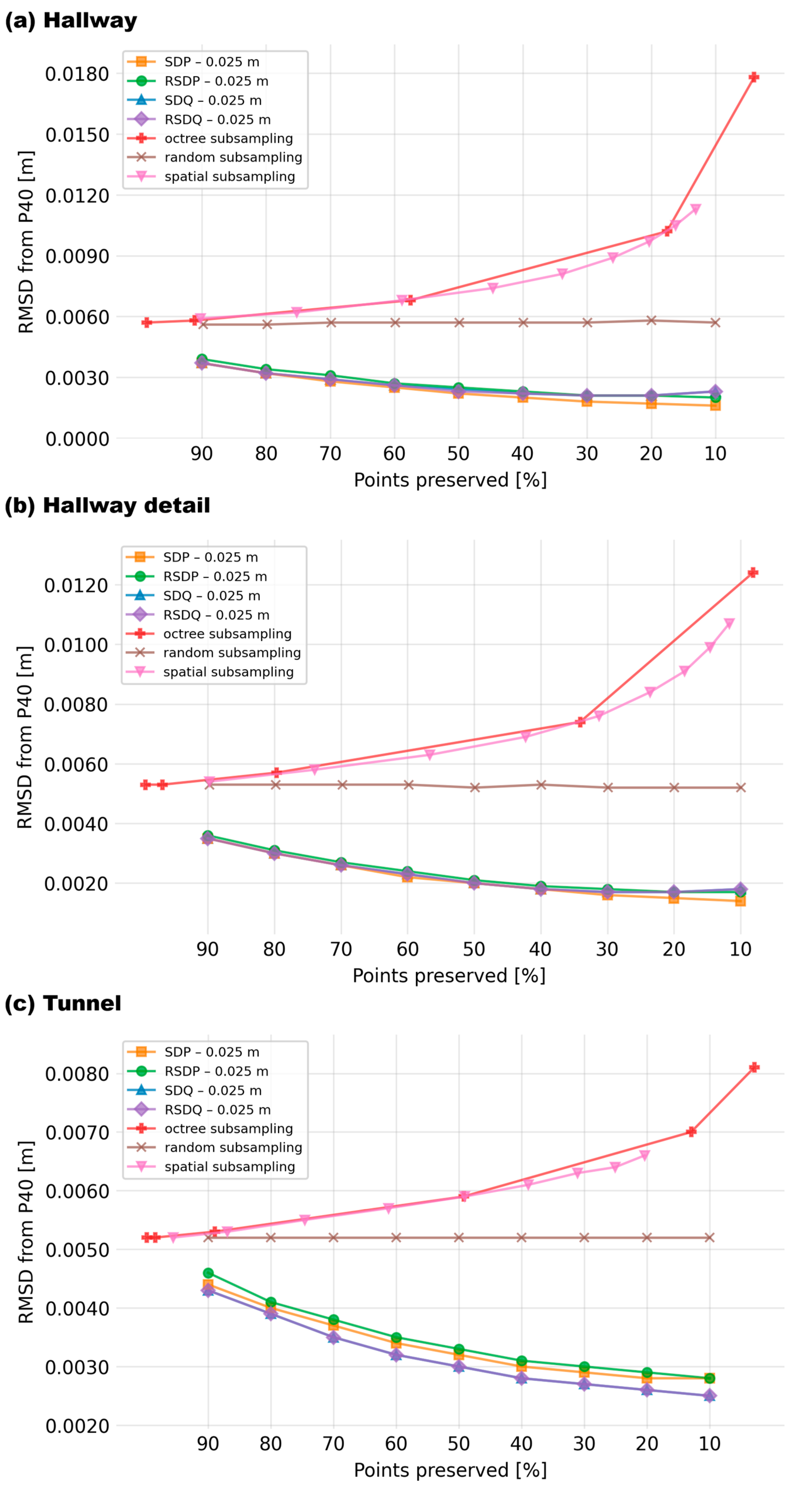
Figure A6.
RMSDs acquired after different degrees of filtering with standard filtering/subsampling approaches and with the novel approach introduced in this study scanned with ZEB Horizon in different scenes – (a) Hallway, (b) Hallway detail, (c) Tunnel.
Figure A6.
RMSDs acquired after different degrees of filtering with standard filtering/subsampling approaches and with the novel approach introduced in this study scanned with ZEB Horizon in different scenes – (a) Hallway, (b) Hallway detail, (c) Tunnel.
Appendix D
Table A2.
Improvement in accuracy (RMSD relative to the reference cloud) after subsampling to 10% of the original cloud using the best-performing algorithm for the respective scanner-scene combination (scanner Emesent Hovermap ST-X).
Table A2.
Improvement in accuracy (RMSD relative to the reference cloud) after subsampling to 10% of the original cloud using the best-performing algorithm for the respective scanner-scene combination (scanner Emesent Hovermap ST-X).
| Scanner | Scene | Method | Original RMSD [mm] | Final RMSD [mm] |
% of original RMSD |
|---|---|---|---|---|---|
| Emesent Hovermap ST-X | Hallway | SDQ, RSDQ | 5.3 | 1.6 | 30.2 |
| Hallway detail | SDP, RSDQ | 6.2 | 1.6 | 24.2 | |
| Tunnel | SDQ, RSDQ | 5.0 | 2.3 | 46.0 | |
| FARO Orbis | Hallway | SDP | 5.7 | 1.6 | 28.1 |
| Hallway detail | SDP | 5.3 | 1.4 | 26.4 | |
| Tunnel | SDQ, RSDQ | 5.2 | 2.5 | 48.1 | |
| ZEB Horizon | Hallway | SDP | 9.8 | 4.0 | 40.8 |
| Hallway detail | SDP | 10.2 | 3.3 | 32.4 | |
| Tunnel | SDQ, RSDQ | 12.6 | 7.0 | 55.6 |
References
- Singh, S.K.; Banerjee, B.P.; Raval, S. A Review of Laser Scanning for Geological and Geotechnical Applications in Underground Mining. International Journal of Mining Science and Technology 2022, 33, 133–154. [CrossRef]
- Gharineiat, Z.; Kurdi, F.T.; Henny, K.; Gray, H.; Jamieson, A.; Reeves, N. Assessment of NAVVIS VLX and BLK2GO SLAM Scanner Accuracy for Outdoor and Indoor Surveying Tasks. Remote Sensing 2024, 16, 3256. [CrossRef]
- Keitaanniemi, A.; Kukko, A.; Virtanen, J.-P.; Vaaja, M.T. Measurement Strategies for Street-Level SLAM Laser Scanning of Urban Environments. The Photogrammetric Journal of Finland/the Photogrammetric Journal of Finland 2020, 27, 1–19. [CrossRef]
- Křemen, T.; Michal, O.; Jiřikovský, T.; Kuric, I.: Long-Distance SLAM Scanning of Mine Tunnel - Testing of Precision and Accuracy of Emesent Hovermap ST-X. Acta Montanistica Slovaca 2024, 29, 630–642. [CrossRef]
- Běloch, L.; Pavelka, K. Optimizing Mobile Laser Scanning Accuracy for Urban Applications: A Comparison by Strategy of Different Measured Ground Points. Appl. Sci. 2024, 14, 3387. [CrossRef]
- Chrbolková, A.; Štroner, M.; Urban, R.; Michal, O.; Křemen, T.; Braun, J. A Comparative Study of Indoor Accuracies Between SLAM and Static Scanners. Appl. Sci. 2025, 15, 8053. [CrossRef]
- Štroner, M.; Urban, R.; Křemen, T.; Braun, J.; Michal, O.; Jiřikovský, T.: Scanning the underground: Comparison of the accuracies of SLAM and static laser scanners in a mine tunnel. Measurement. 2025, 242(242), ISSN 1873-412X.
- Urban, R.; Štroner, M.; Křemen, T.; Braun, J.; Kovanič, L.; Blišťan, P.; Peťovský, P.; Topitzer, B.: Testing the accuracy and characteristics of data acquired using DJI Zenmuse L1 and L2 lidar systems and photogrammetric data acquired using DJI Zenmuse P1 in a quarry environment. European Journal of Remote Sensing. 2025, 58(1), ISSN 2279-7254.
- Štroner, M.; Urban, R.; Křemen, T.; Braun, J. UAV DTM Acquisition in a Forested Area – Comparison of Low-Cost Photogrammetry (DJI Zenmuse P1) and LiDAR Solutions (DJI Zenmuse L1). European Journal of Remote Sensing 2023, 56. [CrossRef]
- Boltcheva, D.; Lévy, B. Surface Reconstruction by Computing Restricted Voronoi Cells in Parallel. Computer-Aided Design 2017, 90, 123–134. [CrossRef]
- Hanocka, R.; Metzer, G.; Giryes, R.; Cohen-Or, D. Point2Mesh. ACM Transactions on Graphics 2020, 39. [CrossRef]
- F. Williams, T. Schneider, C. Silva, D. Zorin, J. Bruna and D. Panozzo, "Deep Geometric Prior for Surface Reconstruction," 2019 IEEE/CVF Conference on Computer Vision and Pattern Recognition (CVPR), Long Beach, CA, USA, 2019, pp. 10122-10131. [CrossRef]
- Maglo, A.; Lavoué, G.; Dupont, F.; Hudelot, C. 3D Mesh Compression. ACM Computing Surveys 2015, 47, 1–41. [CrossRef]
- Luebke, D.P. A Developer’s Survey of Polygonal Simplification Algorithms. IEEE Computer Graphics and Applications 2001, 21, 24–35. [CrossRef]
- Bernardini, F.; Mittleman, J.; Rushmeier, H.; Silva, C.; Taubin, G. The Ball-Pivoting Algorithm for Surface Reconstruction. IEEE Transactions on Visualization and Computer Graphics 1999, 5, 349–359. [CrossRef]
- Vitter, J.S. Faster Methods for Random Sampling. Communications of the ACM 1984, 27, 703–718. [CrossRef]
- R. B. Rusu and S. Cousins, "3D is here: Point Cloud Library (PCL)," 2011 IEEE International Conference on Robotics and Automation, Shanghai, China, 2011, pp. 1-4. [CrossRef]
- Moenning C, Dodgson NA. Fast marching farthest point sampling. Cambridge: University of Cambridge, Computer Laboratory; 2003.
- Štroner, M.; Křemen, T.; Urban, R. Progressive Dilution of Point Clouds Considering the Local Relief for Creation and Storage of Digital Twins of Cultural Heritage. Appl. Sci. 2022, 12, 11540. [CrossRef]
- Gong, M.; Zhang, Z.; Zeng, D. A New Simplification Algorithm for Scattered Point Clouds with Feature Preservation. Symmetry 2021, 13, 399. [CrossRef]
- Zhang, K.; Qiao, S.; Wang, X.; Yang, Y.; Zhang, Y. Feature-Preserved Point Cloud Simplification Based on Natural Quadric Shape Models. Appl. Sci. 2019, 9, 2130. [CrossRef]
- Lee, K.H.; Woo, H.; Suk, T. Data Reduction Methods for Reverse Engineering. The International Journal of Advanced Manufacturing Technology 2001, 17, 735–743. [CrossRef]
- Xu, X.; Li, K.; Ma, Y.; Geng, G.; Wang, J.; Zhou, M.; Cao, X. Feature-Preserving Simplification Framework for 3D Point Cloud. Scientific Reports 2022, 12, 9450. [CrossRef]
- Leal, E.; Sanchez-Torres, G.; Branch-Bedoya, J.W.; Abad, F.; Leal, N. A Saliency-Based Sparse Representation Method for Point Cloud Simplification. Sensors 2021, 21, 4279. [CrossRef]
- O. Dovrat, I. Lang and S. Avidan, "Learning to Sample," 2019 IEEE/CVF Conference on Computer Vision and Pattern Recognition (CVPR), Long Beach, CA, USA, 2019, pp. 2755-2764. [CrossRef]
- E. Nezhadarya, E. Taghavi, R. Razani, B. Liu and J. Luo, "Adaptive Hierarchical Down-Sampling for Point Cloud Classification," 2020 IEEE/CVF Conference on Computer Vision and Pattern Recognition (CVPR), Seattle, WA, USA, 2020, pp. 12953-12961. [CrossRef]
- ZHANG, Dongbo; LU, Xuequan; QIN, Hong a HE, Ying. Pointfilter: Point Cloud Filtering via Encoder-Decoder Modeling. Online. IEEE Transactions on Visualization and Computer Graphics. 2021, vol. 27, no. 3, p. 2015-2027. ISSN 1077-2626. [CrossRef]
- ŠTRONER, Martin; BOUŠEK, Martin; KUČERA, Jakub; VÁCHOVÁ, Hana a URBAN, Rudolf. Multi-Size Voxel Cube (MSVC) Algorithm—A Novel Method for Terrain Filtering from Dense Point Clouds Using a Deep Neural Network. Online. Remote Sensing. 2025, vol. 17, no. 4. ISSN 2072-4292. [CrossRef]
- QI, Charles R.; SU, Hao; MO, Kaichun and GUIBAS, Leonidas J. PointNet: Deep Learning on Point Sets for 3D Classification and Segmentation. Online. 2017. [CrossRef]
- LUO, Shitong a HU, Wei. Differentiable Manifold Reconstruction for Point Cloud Denoising. Online. Proceedings of the 28th ACM International Conference on Multimedia. 2020, p. 1330-1338. ISBN 9781450379885. [CrossRef]
- RAKOTOSAONA, Marie-Julie; LA BARBERA, Vittorio; GUERRERO, Paul; MITRA, Niloy J. a OVSJANIKOV, Maks. PointCleanNet: Learning to Denoise and Remove Outliers from Dense Point Clouds. Online. Computer Graphics Forum. 2020, vol. 39, no. 1, p. 185-203. ISSN 0167-7055. [CrossRef]
- Removing outliers using a StatisticalOutlierRemoval filter. Online. Point Cloud Library documentation: https://pcl.readthedocs.io/projects/tutorials/en/latest/statistical_outlier.html.
- M. Alexa, J. Behr, D. Cohen-Or, S. Fleishman, D. Levin and C. T. Silva, "Computing and rendering point set surfaces," in IEEE Transactions on Visualization and Computer Graphics, vol. 9, no. 1, pp. 3-15, Jan.-March 2003. [CrossRef]
- AMBROSINO, Antonella; DI BENEDETTO, Alessandro a FIANI, Margherita. Hybrid Denoising Algorithm for Architectural Point Clouds Acquired with SLAM Systems. Online. Remote Sensing. 2024, vol. 16, no. 23. ISSN 2072-4292. [CrossRef]
Figure 1.
Comparison of the profiles (cross-sections in the perpendicular direction to the surface) from a SLAM scanner Emesent Hovermap ST-X (red) and a reference cloud from a static terrestrial scanner Leica P40 (blue).
Figure 1.
Comparison of the profiles (cross-sections in the perpendicular direction to the surface) from a SLAM scanner Emesent Hovermap ST-X (red) and a reference cloud from a static terrestrial scanner Leica P40 (blue).
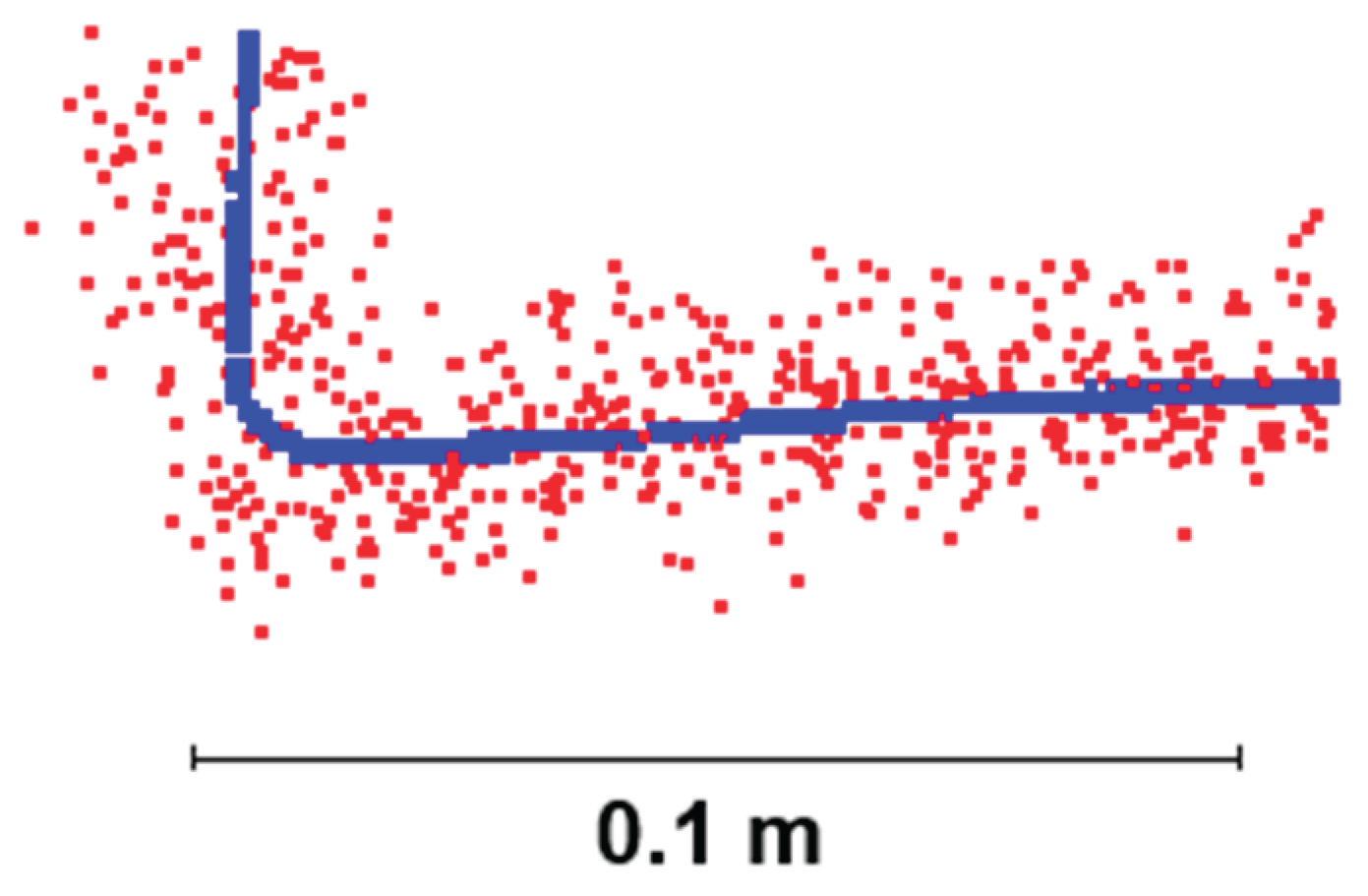
Figure 2.
A simplified (two-dimensional) depiction of the spherical neighborhood and the principle of the SDP method (Standardized distance to the planar surface). The evaluated characteristic is then calculated as the distance of the point of interest (red) from the plane fitted to all points in the spherical neighborhood, divided by the standard deviation of all points in the neighborhood relative to the fitted plane.
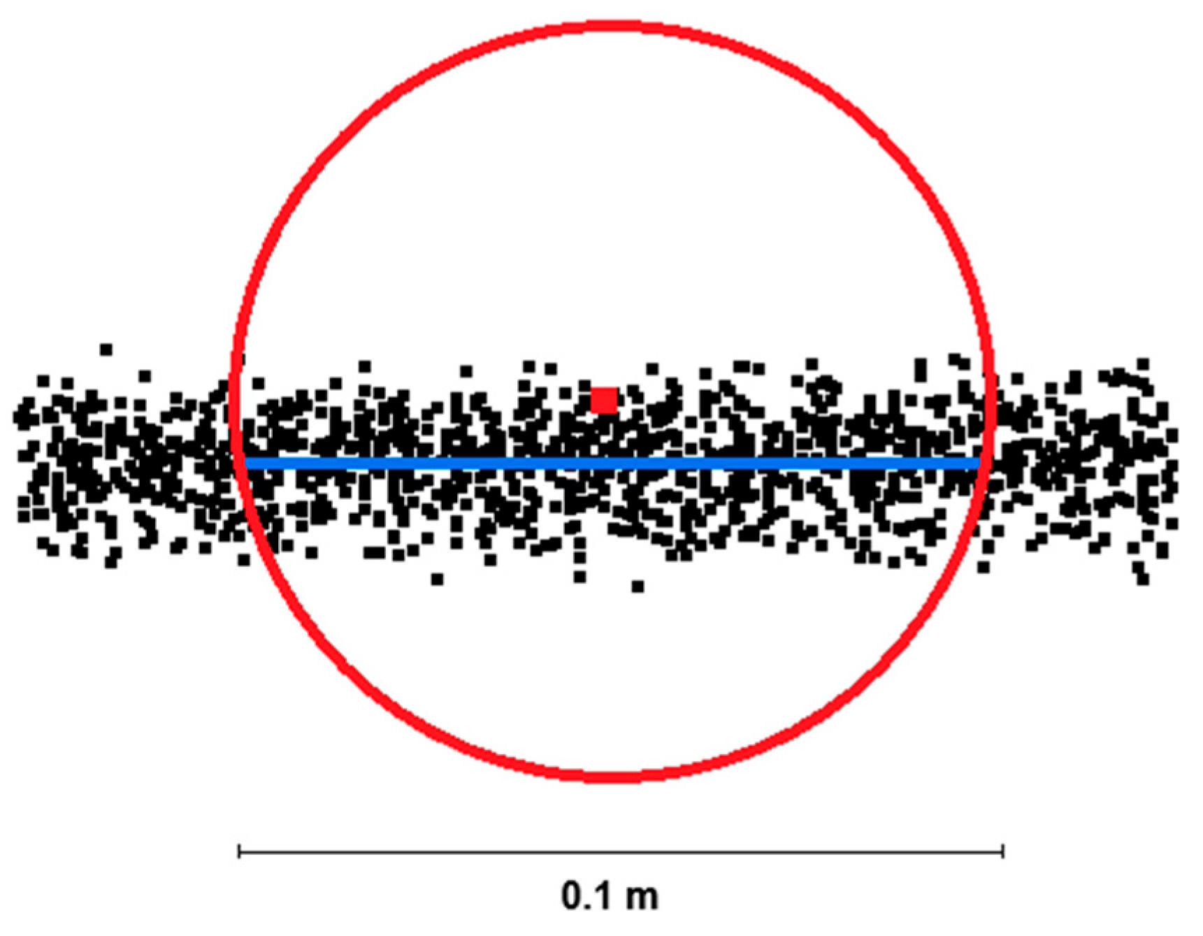
Figure 3.
A simplified (2D) depiction of the RSDP (Ratio of standard deviations from the planar surface) algorithm. The value is calculated as the ratio of standard deviations of all points within the neighborhood calculated relative to the fitted plane forced to pass through the investigated point (green) and relative to the plane representing the best possible fit (blue).
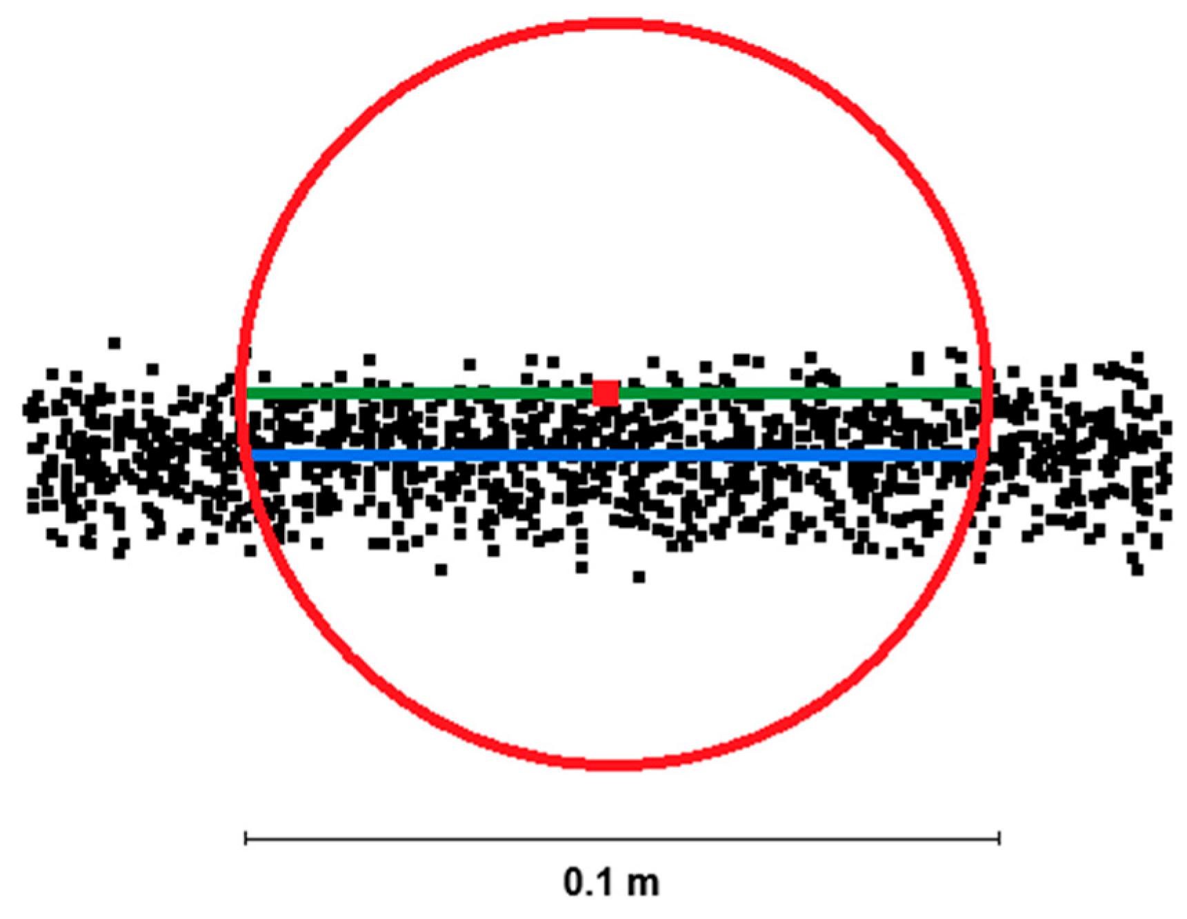
Figure 4.
A simplified (2D) depiction of the benefits brought to the evaluation by replacing the planar surface (b) with a quadratic one (a).
Figure 4.
A simplified (2D) depiction of the benefits brought to the evaluation by replacing the planar surface (b) with a quadratic one (a).
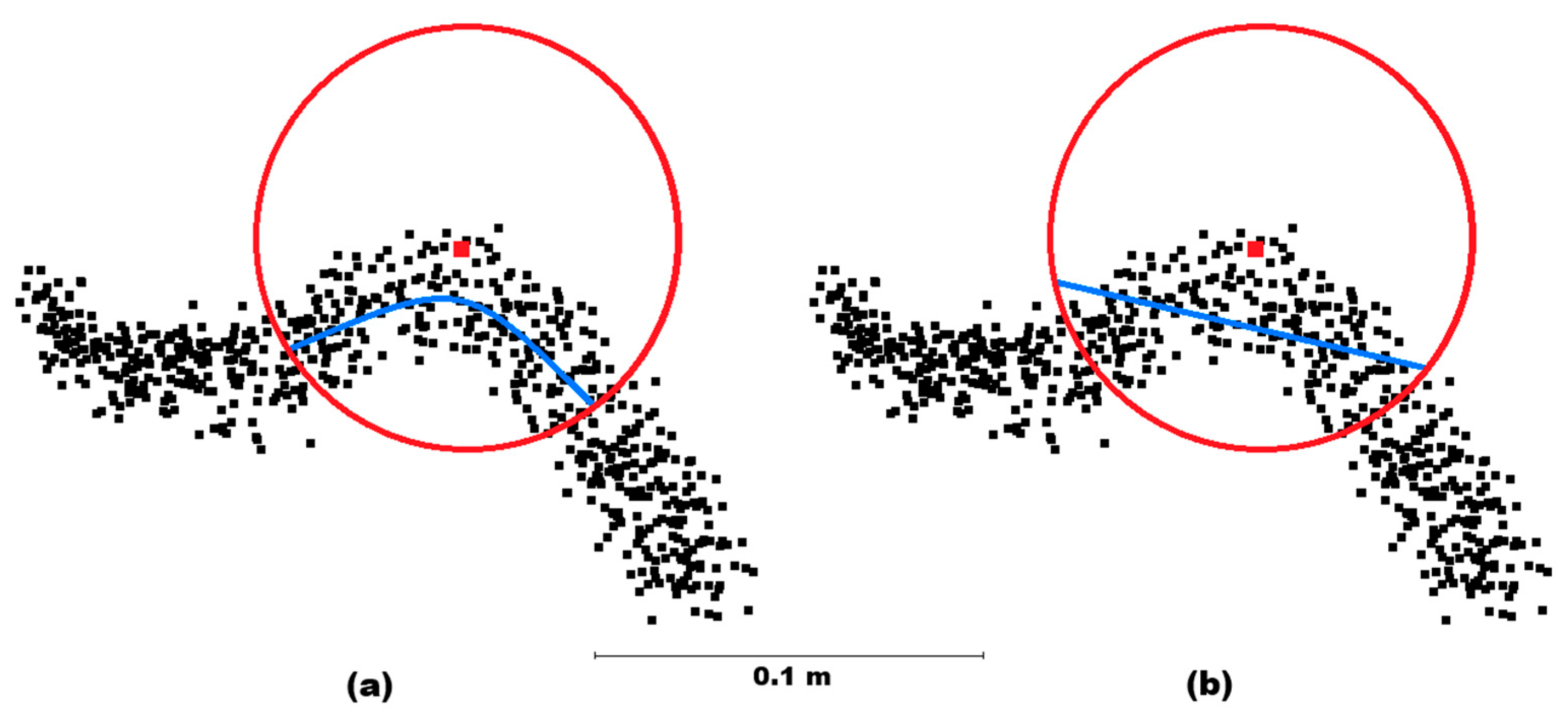
Figure 5.
A simplified (2D) depiction of the principle of the RSDQ (Ratio of standard deviations relative to quadratic surfaces) method, with the blue line indicating the best possible quadratic surface and the green line representing the best possible quadratic surface forced to pass through the point of interest.
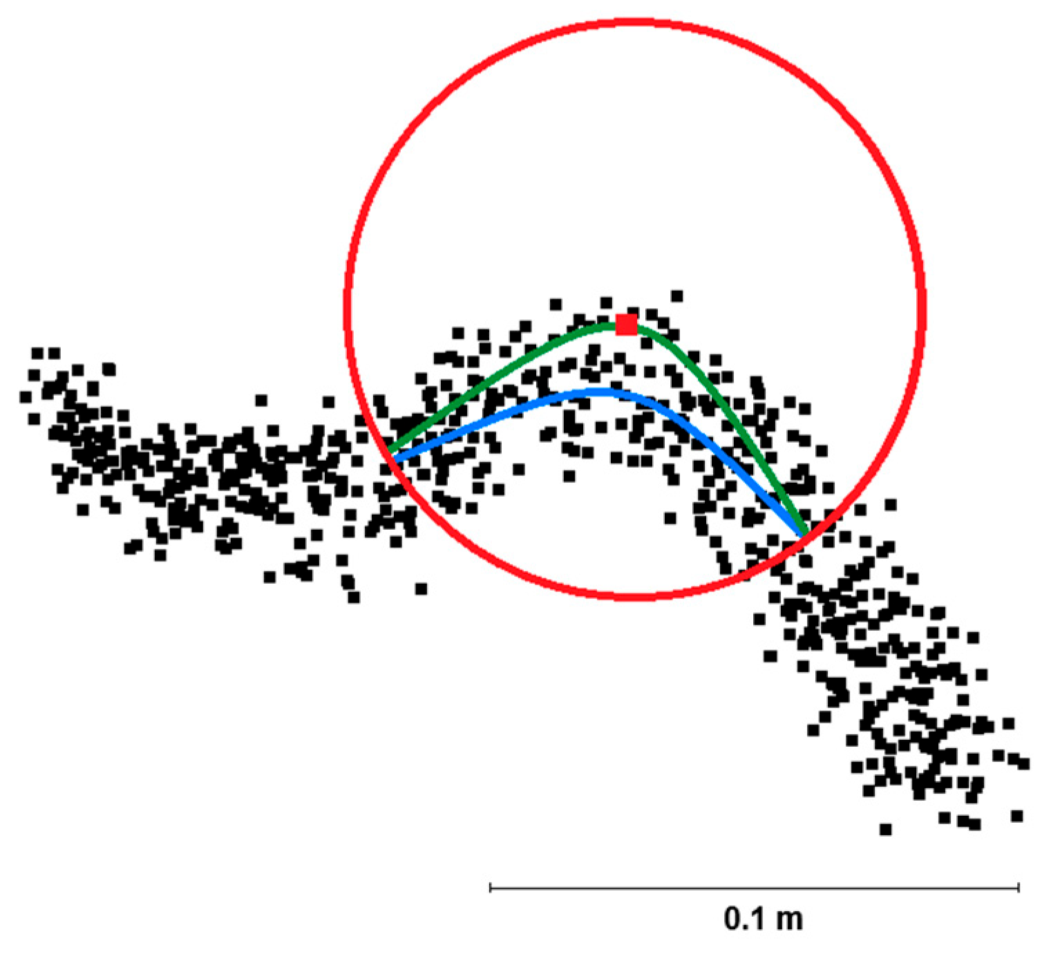
Figure 6.
Section through a part of the point cloud with colors of points indicating the values of the Standardized distance to quadratic surface (SDQ) metric calculated for a spherical neighborhood of 0.05 m.
Figure 6.
Section through a part of the point cloud with colors of points indicating the values of the Standardized distance to quadratic surface (SDQ) metric calculated for a spherical neighborhood of 0.05 m.
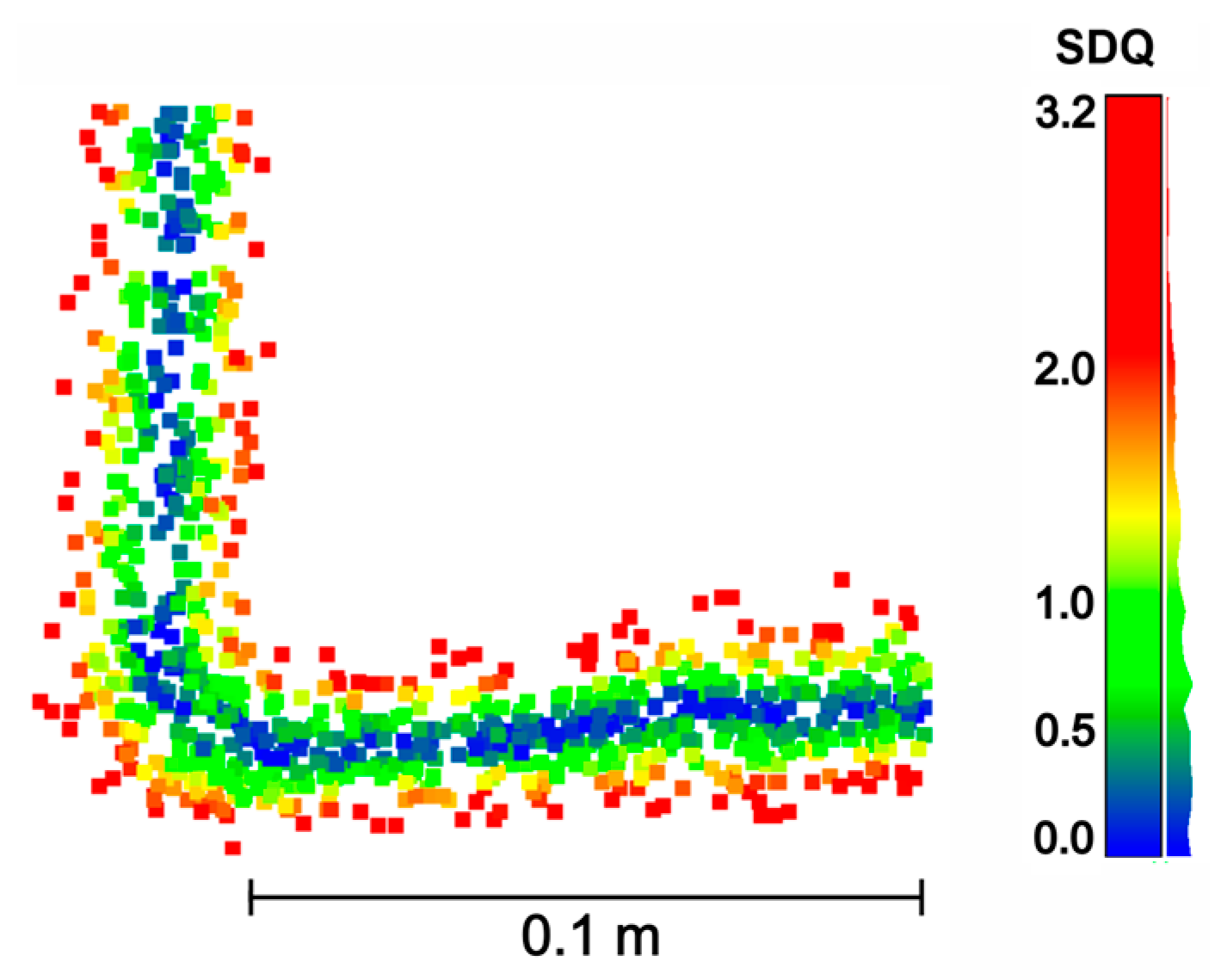
Figure 7.
The scenes used for evaluation: (a) Hallway, (b) Hallway detail, (c) Tunnel; note that the missing (white) parts were removed from analysis as they were not properly scanned by the reference static terrestrial scanner due to shadowing effects.
Figure 7.
The scenes used for evaluation: (a) Hallway, (b) Hallway detail, (c) Tunnel; note that the missing (white) parts were removed from analysis as they were not properly scanned by the reference static terrestrial scanner due to shadowing effects.
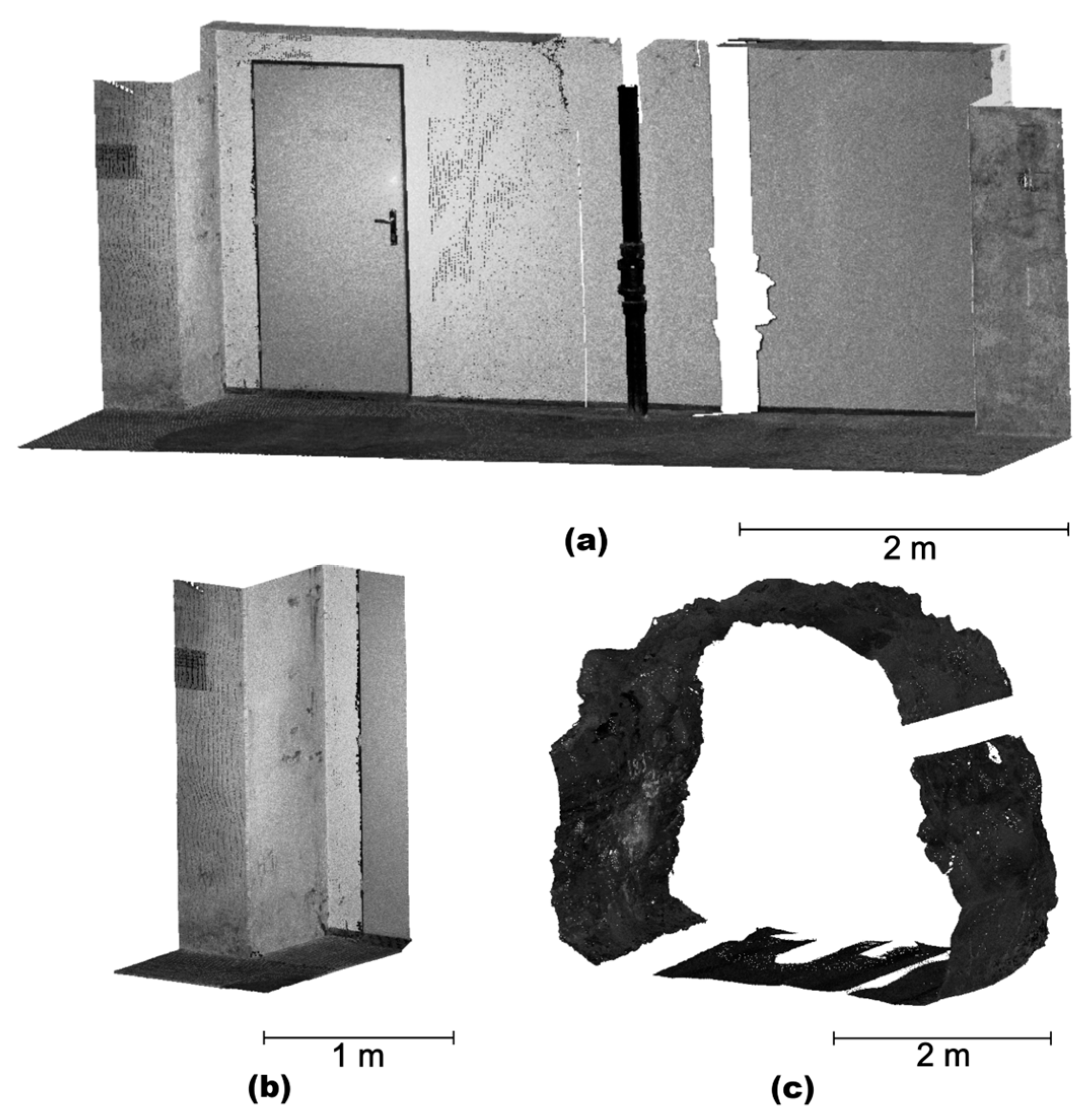
Figure 8.
Plot of RMSDs relative to the reference cloud using the SDQ filtering method for the Hallway (detail) scene scanned using the Emesent Hovermap ST-X scanner for individual sizes (radii) of the spherical neighborhood.
Figure 8.
Plot of RMSDs relative to the reference cloud using the SDQ filtering method for the Hallway (detail) scene scanned using the Emesent Hovermap ST-X scanner for individual sizes (radii) of the spherical neighborhood.
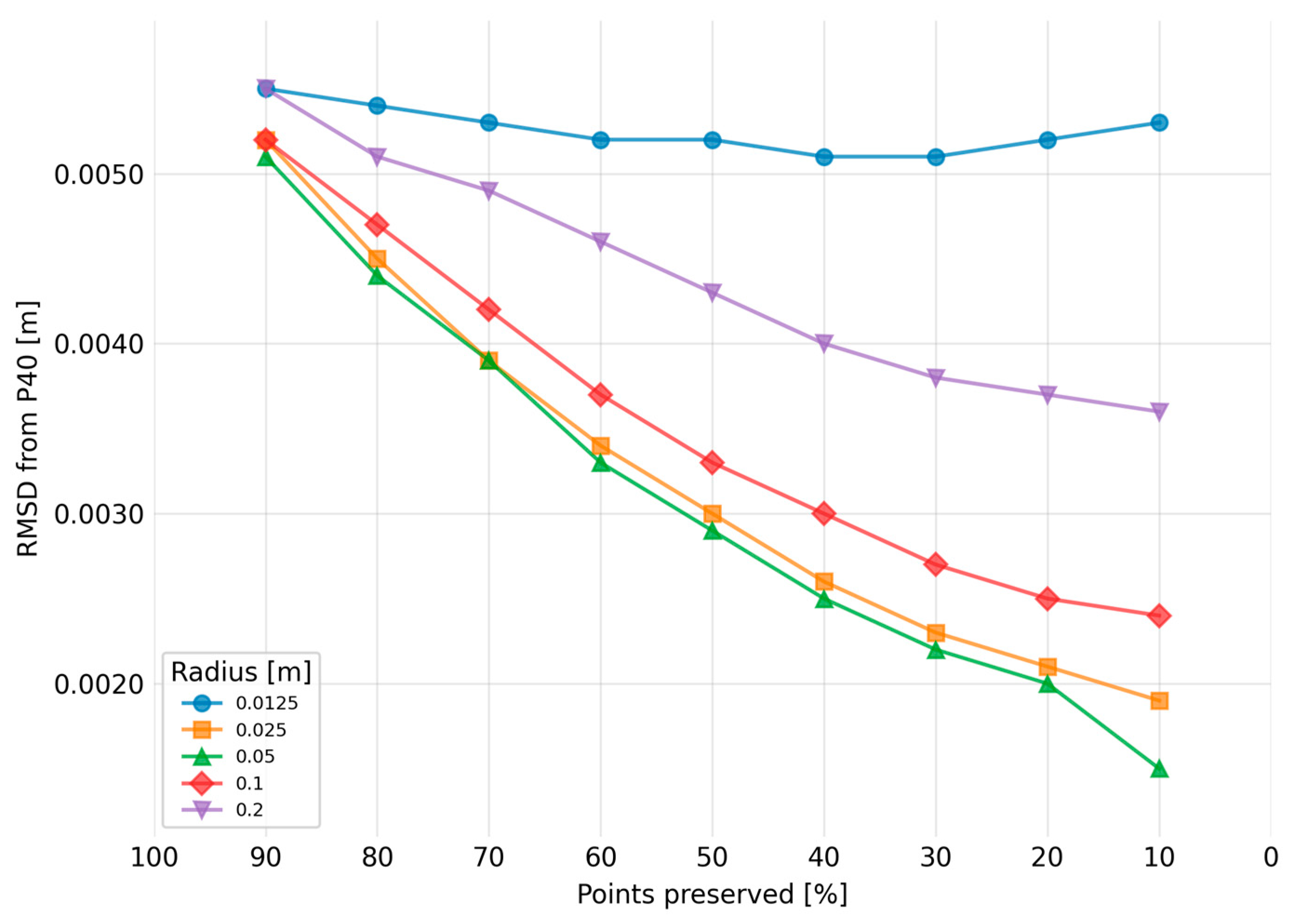
Figure 9.
Point cloud depicting a corner with point quality color-coded according to the SDQ parameter for two sizes of the spherical neighborhood: (a) radius of 0.025 and (b) radius of 0.2 m. Blue points will be retained after filtering; note the fewer and incorrectly identified points kept in the region of the edge with larger spherical surroundings.
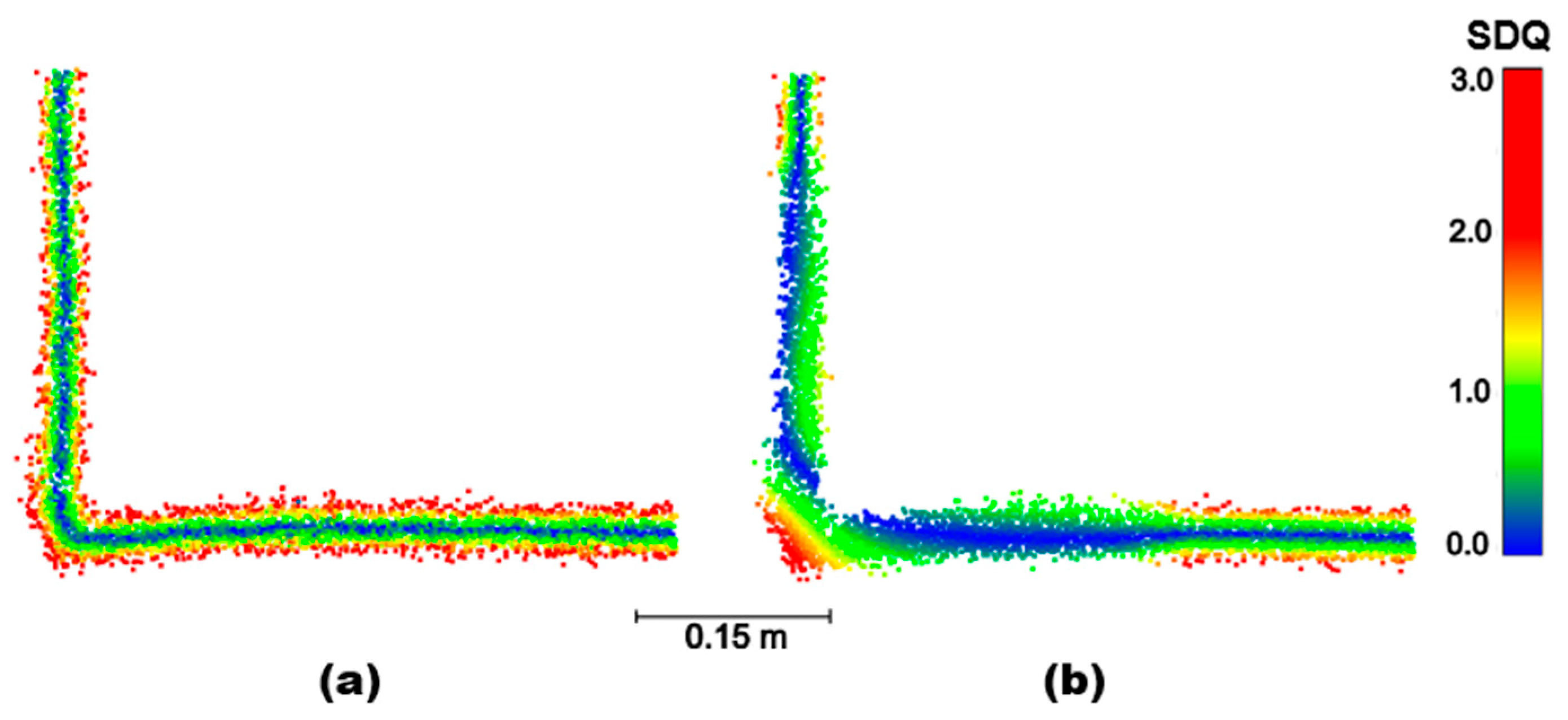
Figure 11.
An example of the profile of (a) an unfiltered cloud and (b) cloud after filtering with remaining outliers (scene Hallway, FARO Orbis, SDQ filtering with 20% points preserved, spherical neighborhood 0.05 m).
Figure 11.
An example of the profile of (a) an unfiltered cloud and (b) cloud after filtering with remaining outliers (scene Hallway, FARO Orbis, SDQ filtering with 20% points preserved, spherical neighborhood 0.05 m).

Figure 12.
(a) A part of the point cloud (Hallway, Emesent Hovermap) with the highlighted profile and the profiles (b) from the original point cloud with 742,846 points and (c) from the filtered point cloud (SDQ, spherical neighborhood of 0.05 m), preserving only 10% of points.
Figure 12.
(a) A part of the point cloud (Hallway, Emesent Hovermap) with the highlighted profile and the profiles (b) from the original point cloud with 742,846 points and (c) from the filtered point cloud (SDQ, spherical neighborhood of 0.05 m), preserving only 10% of points.
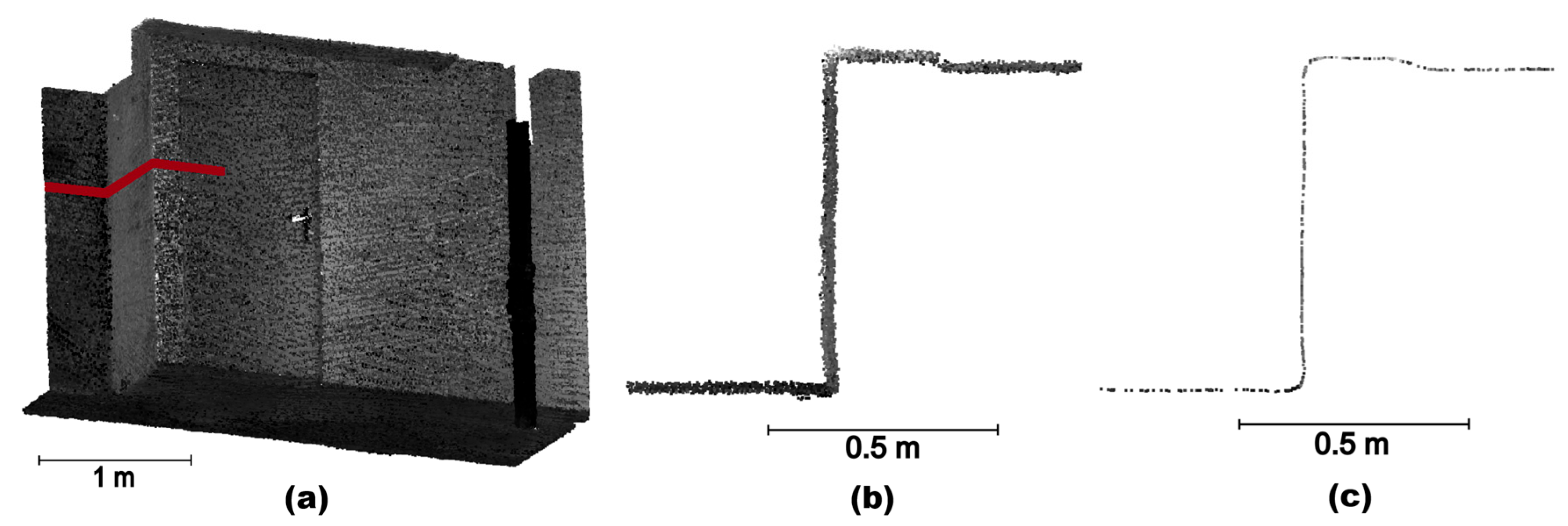
Figure 13.
Mean point-to-point distances resulting from individual filtering cut-offs for (a) all point clouds from individual scanners and scenes, (b) point clouds from the Hallway scene comparing all three scanners. Note that the curves only indicate distances between points; accuracies (RMSDs compared with P40) are indicated by the numbers at individual points (SDQ filtering, spherical neighborhood 0.05 m).
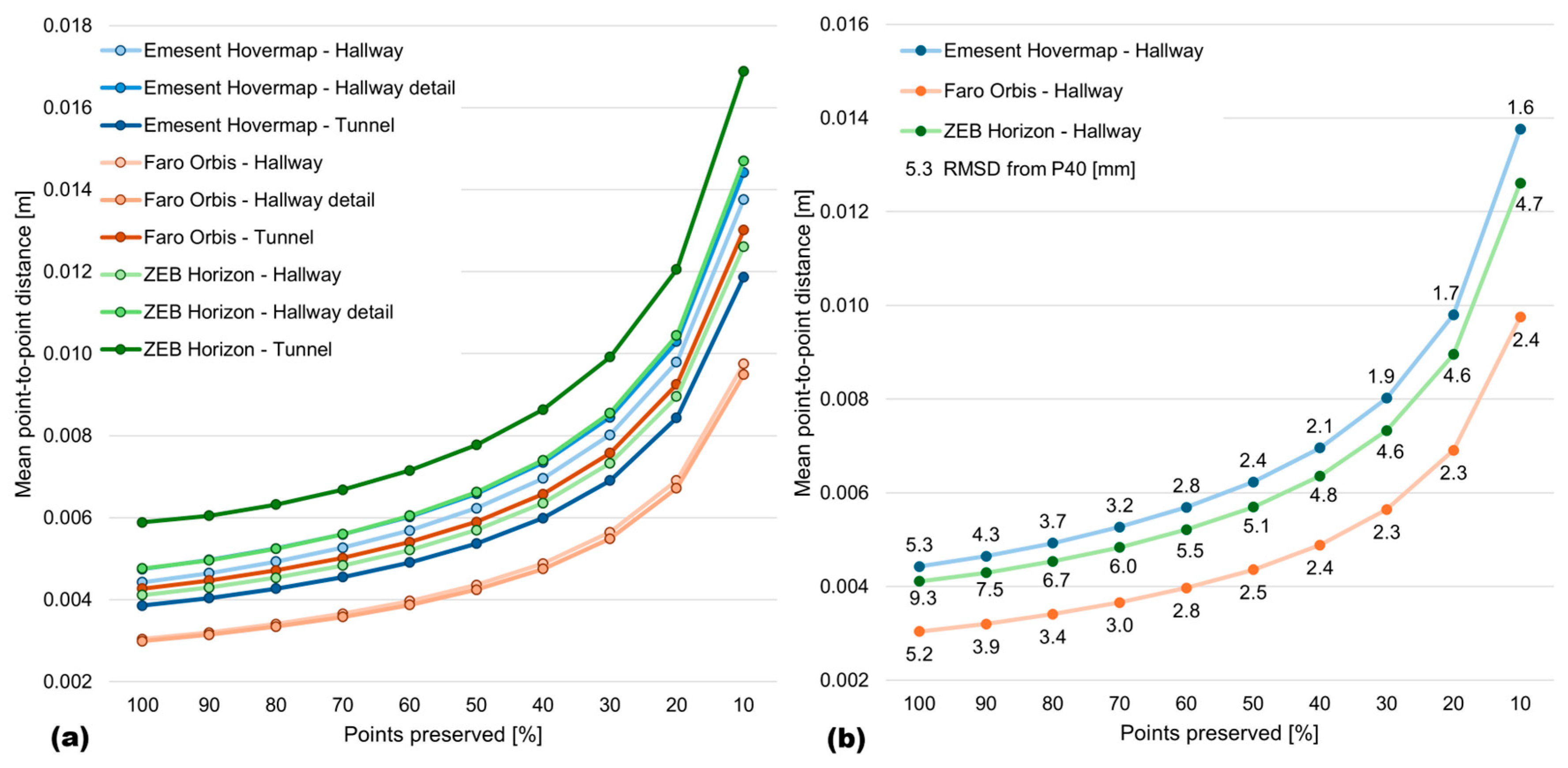
Figure 14.
RMSDs acquired after different degrees of filtering with standard filtering/subsampling approaches and with the novel approach introduced in this study (scene Hallway, Emesent Hovermap ST-X).
Figure 14.
RMSDs acquired after different degrees of filtering with standard filtering/subsampling approaches and with the novel approach introduced in this study (scene Hallway, Emesent Hovermap ST-X).
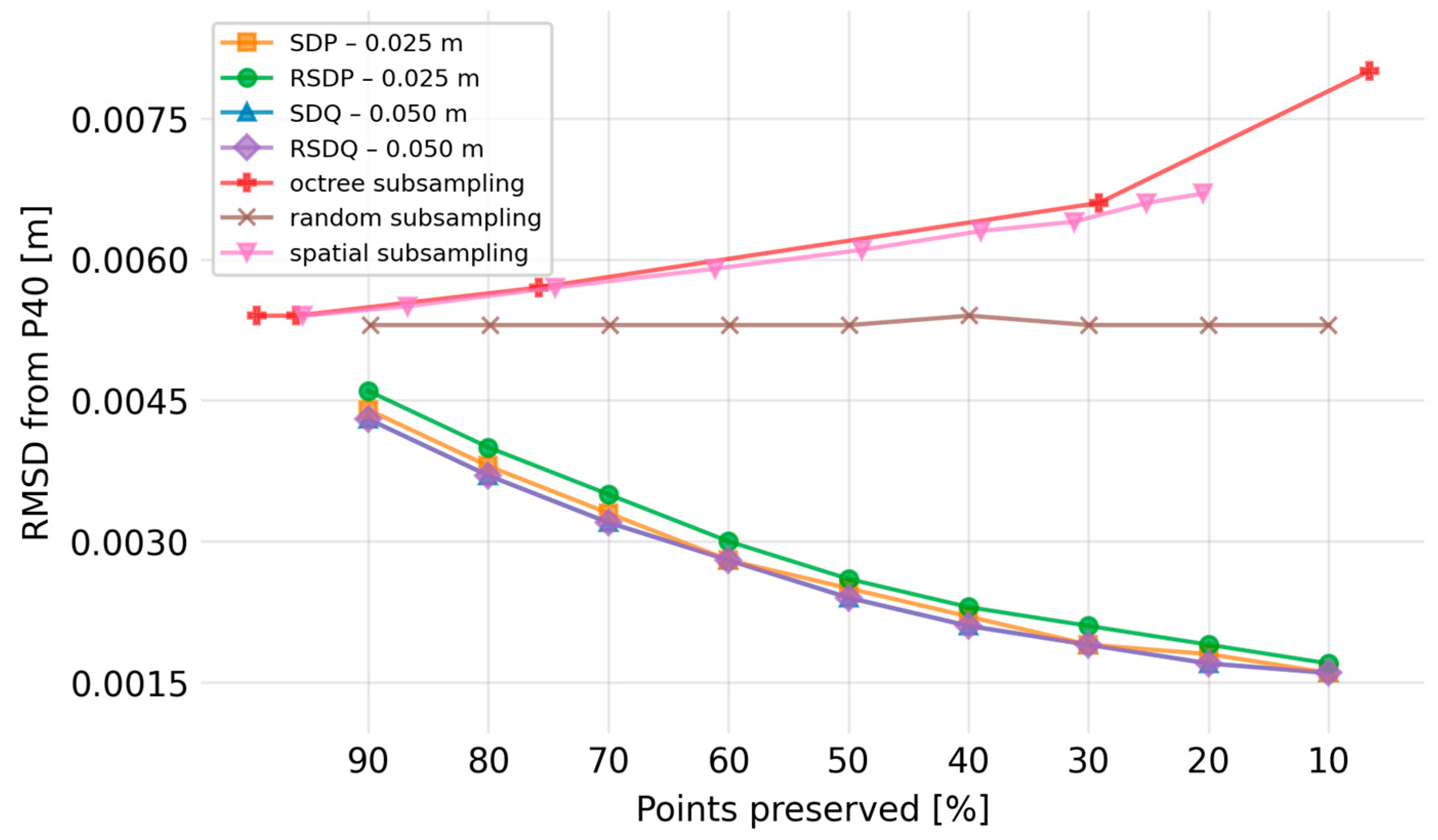
Figure 15.
RMSDs relative to the reference cloud resulting from individual filtering cut-offs (preserving 90% to 10% of the points) using the best-performing spherical neighborhood and all four newly proposed noise filtering methods. Each row of panels shows results of scanning with one scanner (Emesent Hovermap ST-X – panels (a-c); Faro Orbis – panels (d-f); ZEB Horizon – panels (g-i)), each column shows results for a different scene (Hallway – (a, d, g); Hallway detail – (b, e, h); Tunnel – (c, f, i)).
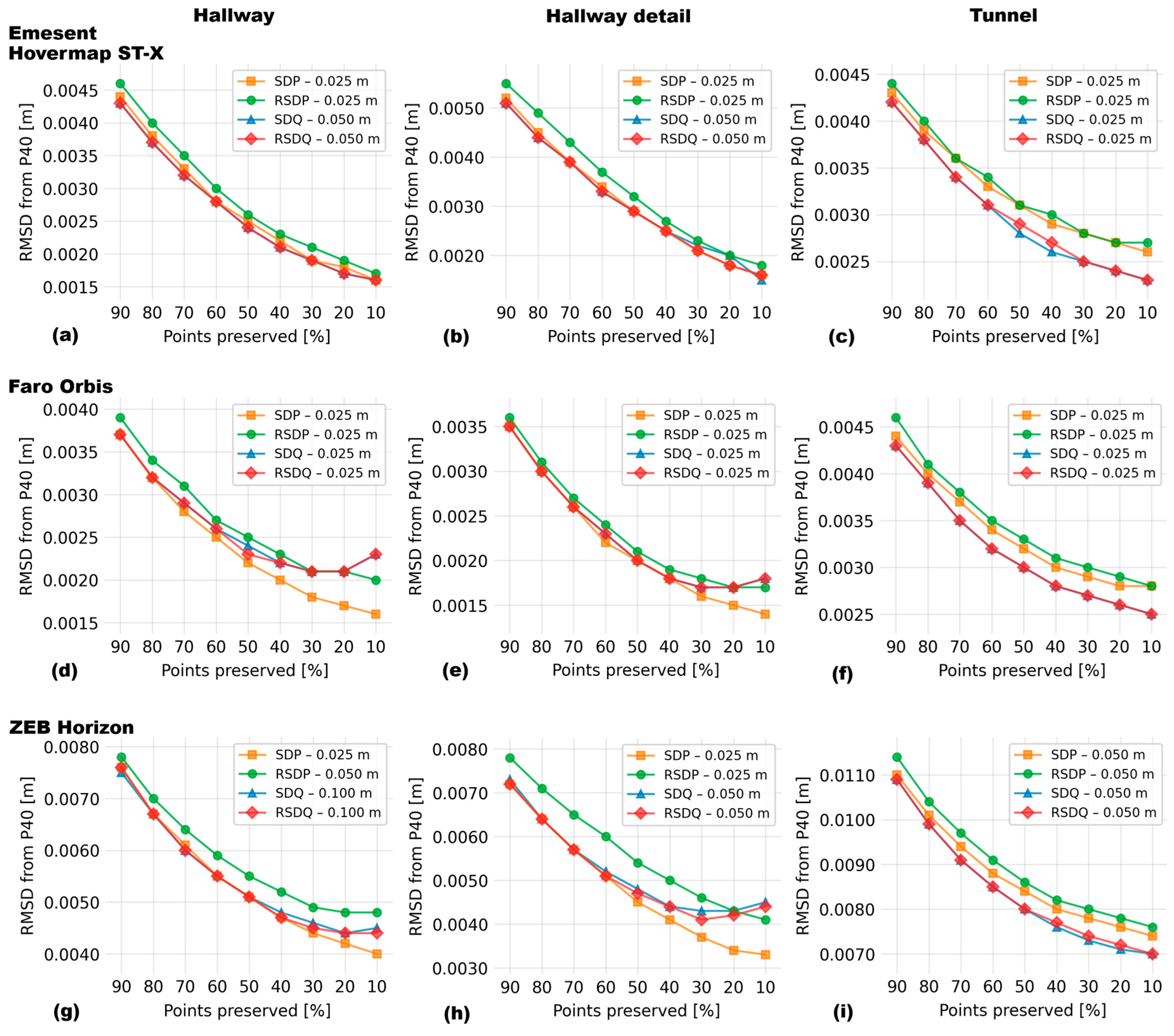
Table 1.
Parameters of standard subsampling methods implemented in CloudCompare used for the comparison with proposed algorithms.
Table 1.
Parameters of standard subsampling methods implemented in CloudCompare used for the comparison with proposed algorithms.
| Standard subsampling method | Used parameters |
|---|---|
| Octree subsampling level | 12, 11, 10, 9, 8, 7, 6 |
| Random subsampling [%] | 10, 20, 30, 40, 50, 60, 70, 80, 90 |
| Spatial subsampling [mm] | 2, 3, 4, 5, 6, 7, 8, 9, 10 |
Table 2.
Parameters of the used point clouds.
| Scene | Point cloud dimensions (width x length x height) [m] |
Scanner | Number of points | Average density [points/m2] |
|---|---|---|---|---|
| Hallway | 6.2 × 2.1 x 2.3 | Emesent Hovermap ST-X | 1,451,730 | 51,137 |
| FARO Orbis | 2,523,183 | 108,365 | ||
| ZEB Horizon | 1,470,007 | 59,163 | ||
| Leica P40 | 25,887,573 | 1,214,220 | ||
| Hallway detail | 0.9 x 2.1 x 2.0 | Emesent Hovermap ST-X | 186,724 | 44,516 |
| FARO Orbis | 407,653 | 112,071 | ||
| ZEB Horizon | 162,429 | 44,151 | ||
| Leica P40 | 5,414,767 | 1,287,852 | ||
| Tunnel | 4.3 x 1.9 x 3.6 | Emesent Hovermap ST-X | 1,745,018 | 67,273 |
| FARO Orbis | 1,297,448 | 54,884 | ||
| ZEB Horizon | 731,227 | 28,874 | ||
| Leica P40 | 31,132,854 | 1,223,351 |
Table 3.
The RMSDs of the original point clouds and best-performing spherical neighborhoods for individual scanner-method-scene combinations.
Table 3.
The RMSDs of the original point clouds and best-performing spherical neighborhoods for individual scanner-method-scene combinations.
| Scanner | Scene | RMSD of the unfiltered point cloud [m] | Radius for SDP1 [m] | Radius for RSDP2 [m] | Radius for SDQ3 [m] | Radius for RSDQ4 [m] |
|---|---|---|---|---|---|---|
| Emesent Hovermap ST-X | Hallway | 0.0053 | 0.025 | 0.025 | 0.050 | 0.050 |
| Hallway detail | 0.0062 | 0.025 | 0.025 | 0.050 | 0.050 | |
| Tunnel | 0.0050 | 0.025 | 0.025 | 0.025 | 0.025 | |
| FARO Orbis | Hallway | 0.0057 | 0.025 | 0.025 | 0.025 | 0.025 |
| Hallway detail | 0.0053 | 0.025 | 0.025 | 0.025 | 0.025 | |
| Tunnel | 0.0052 | 0.025 | 0.025 | 0.025 | 0.025 | |
| ZEB Horizon | Hallway | 0.0098 | 0.025 | 0.050 | 0.100 | 0.100 |
| Hallway detail | 0.0102 | 0.025 | 0.025 | 0.050 | 0.050 | |
| Tunnel | 0.0126 | 0.050 | 0.050 | 0.050 | 0.050 |
1 standardized distance to plane, 2 ratio of standard deviations from the planar surfaces, 3 standardized distance to quadratic surface, 4 ratio of standard deviations relative to quadratic surfaces.
Disclaimer/Publisher’s Note: The statements, opinions and data contained in all publications are solely those of the individual author(s) and contributor(s) and not of MDPI and/or the editor(s). MDPI and/or the editor(s) disclaim responsibility for any injury to people or property resulting from any ideas, methods, instructions or products referred to in the content. |
© 2026 by the authors. Licensee MDPI, Basel, Switzerland. This article is an open access article distributed under the terms and conditions of the Creative Commons Attribution (CC BY) license (http://creativecommons.org/licenses/by/4.0/).
Copyright: This open access article is published under a Creative Commons CC BY 4.0 license, which permit the free download, distribution, and reuse, provided that the author and preprint are cited in any reuse.


