Submitted:
09 January 2026
Posted:
12 January 2026
You are already at the latest version
Abstract
To enhance the anti-jamming performance and operational reliability of drones, this paper presents the design, fabrication, and measurement of a novel polarization-reconfigurable metasurface antenna that meets these demands. The design process is guided systematically by characteristic mode analysis, in which the modal significance coefficient is used as a key tool to predict resonant frequencies and optimize bandwidth. A major innovation lies in the mechanical rotation mechanism, which enables the antenna to switch between left-hand circular polarization, linear polarization, and right-hand circular polarization, thereby avoiding losses associated with active electronic components. The antenna features a compact geometry of 0.49λ × 0.49λ and delivers strong performance across all polarization states, impedance bandwidth exceeds 29.9%, average gain ranges from 5.1 to 6.0 dBi, and high polarization purity is achieved, with an axial ratio bandwidth >10% in circular polarization modes and cross-polarization discrimination >23 dB in the linear polarization state. Simulated and measured results are in good agreement, confirming the effectiveness and robustness of the proposed design for modern 5G/6G terminals.
Keywords:
metasurface antenna
; polarization reconfigurable
; characteristic mode analysis
; modal significance
; drone terminals
1. Introduction
With the expanding application of unmanned aerial vehicles (UAVs), or drone, the operational reliability of their communication links, particularly anti-jamming capability, has become increasingly critical. Leveraging the polarization characteristics of electromagnetic waves presents a significant technical approach to address such challenges. The polarization properties of antennas, especially the ability to dynamically reconfigure polarization in response to varying operational scenarios—known as polarization reconfigurability—constitute a key research focus in this field. The application scenario is illustrated in Figure 1.
The rapid deployment of 5G and the ongoing evolution towards 6G technology impose increasingly stringent requirements on terminal antennas, compelling a focused research effort on achieving miniaturization, wide impedance bandwidth, high gain, and adaptive functionality within extremely confined spaces. The limited physical size of modern mobile devices necessitates antenna designs that are not only compact but also capable of supporting high data rates and reliable connectivity. Traditional microstrip antennas, while low-profile and easy to integrate, fundamentally struggle to meet these multi-faceted demands due to their inherent limitations in bandwidth, gain, and functional agility [1].
Metasurface antennas, which leverage two-dimensional artificial electromagnetic structures composed of subwavelength unit cells, have emerged as a profoundly promising alternative [2]. They offer a unique combination of a low profile, high integration potential, and exceptional control over wavefronts and polarization states, enabling performance characteristics that are difficult to achieve with conventional designs. Significant research efforts have been directed towards addressing three critical challenges in antenna technology for modern wireless systems [3,4]. The first is miniaturization, which is paramount for integration into compact smart terminals and internet of things (IoT) devices. Techniques such as employing slotting and branch-loading on patches, as well as incorporating defected ground structures (DGS) [5], have been effectively used to reduce antenna size and achieve multi-band operation. The second key area is the generation of circular polarization, which is highly desirable for its robustness against multipath fading and orientation mismatches between transmitting and receiving antennas [6]. It has been proved that metasurfaces is exceptionally capable in this regard. It was often used as superstrates to transform a linearly polarized source into a radiator with wide axial ratio bandwidth [7]. The critical research focus is reconfigurability [8], which allows a single antenna to dynamically adapt to varying channel conditions and communication standards.
Polarization configurability, in particular, is crucial for optimizing signal quality, mitigating interference, and improving compatibility with diverse network infrastructures. Conventional reconfiguration techniques predominantly rely on active components like PIN diodes or varactors [9]. However, these introduce well-documented drawbacks, including insertion loss, design complexity, DC power consumption, and the potential for harmonic radiation [10].
To overcome these limitations, a promising direction is the development of passive, mechanically reconfigurable antennas. The design process for such innovative antennas can be rigorously guided by characteristic mode analysis (CMA) [11], a powerful computational method for analyzing the inherent resonant properties (or characteristic modes) of a conducting structure without the influence of a specific excitation. The modal significance (MS) parameter serves as a central design metric within CMA [12], quantitatively identifying the most significant resonant modes of the metasurface structure. This analytical approach provides deep physical insight and systematically guides the structural evolution towards optimal performance for both miniaturization and multi-polarization generation [13]. Research has demonstrated that CMA can be effectively used to design metasurfaces that excite multiple broadside modes, which is essential for achieving wide impedance bandwidth.
Polarization-reconfigurable antennas represent an advanced form of antenna technology. They can dynamically switch or adjust their polarization states—such as linear or circular polarization—based on the channel environment and interference conditions. This capability allows the antenna to maintain optimal matching with the signal while maximizing interference suppression, which requires intelligent sensing and fast control algorithms.
In this approach, the principal contributions of this paper are as follows.
i) Systematic Design via CMA
The application of CMA and MS analysis to systematically design and optimize a miniaturized metasurface unit cell. This method enables a targeted adjustment of the structure's resonant properties, achieving a significant reduction in operational frequency and ensuring optimal excitation of desired modes for wideband performance.
ii) Low-Loss Polarization Switching
The introduction of a simple yet effective mechanical rotation mechanism applied to the metasurface layer. This passive approach enables low-loss and highly reliable polarization switching among left-hand circular polarization (LHCP), Linear Polarization (LP), and right-hand circular polarization (RHCP) states, effectively eliminating the losses and complexities associated with active electronic components.
iii) Experimental Validation of a High-Performance Antenna
The realization and experimental validation of a compact antenna prototype that demonstrates wide impedance bandwidth (>29.9%), stable gain across all polarization states (5.1 to 6.0 dBi), and high polarization purity. The excellent agreement between simulation and measurement confirms its potential as a robust solution for 5G terminal devices.
This approach aims to bridge the gap between the demanding requirements of modern wireless communication and the limitations of current antenna solutions by presenting a passively reconfigurable metasurface antenna that excels in size, bandwidth, and adaptive functionality. To achieve the above, the paper is structured as follows. Section 2 introduces the design principles, including the theoretical basis of characteristic modes and MS analysis. Section 3 presents simulation results. To verify our newly designed antenna, experimental results and analysis have been provided in Section 4. Finally, we offer conclusions last section.
2. Antenna Design Principles with MS Analysis
2.1. Theoretical Foundation of Characteristic Modes
The theory of characteristic modes provides a deterministic framework for analyzing the modal behavior of a conducting body. It involves solving a weighted eigenvalue equation derived from the method of moments impedance matrix [14].
where Jn is the n-th mode characteristic current, rand X is the real and imaginary parts of the impedance matrix, and λn is the associated eigenvalue. A key derived parameter is the MS defined by
MSn=1/∣1+jλn∣
The MS indicates how easily a mode can be excited. Its value close to 1 signifies a strong, easily excited mode that dominates the radiation at a specific frequency. Since CMA is independent of the feed, it offers profound physical insight into the structure's intrinsic resonances, making it ideal for initial design and optimization.
2.2. CMA-Guided Evolution of the Metasurface Unit Cell
Without generality, the core of the antenna consists of a 4x4 periodic metasurface array. In order to present the metasurface as an antenna’s radiator with polarization transformer, we verify the unit cell changing through four stages, and the CMA method is used. By using CST Microwave Studio's integral equation solver, the evolution of the surface current distribution and MS has been checked. We summarize four stages, as shown in Figure 2 to Figure 13. These figures not only indicate the law of polarization changes with antenna structure changes, but also guide our design.
i) Square Patch
The initial analysis of a simple square patch revealed weak current distributions for the four modes, as shown in Figure 2. While modes 3 and 4 showed orthogonal currents, their radiation pattern for these modes were depicted in Figure 3. We found these patterns almost the same form. The MS peaks were narrow and occurred at a high frequency of approximately 7 GHz, as shown in Figure 4, it is unsuitable for a compact design.
ii) Patch with Corner Cutouts
When cutting off a pair of opposite corners of a square, we can enhance the orthogonal current components. The current distributions and radiation patterns of four model are depicted in Figure 5 and Figure 6, respectively. The MS peaks moved to lower frequency, to about 5.18 GHz (mode 1) and 5.83 GHz (mode 2) with wider bandwidths. However, degenerate modes (modes 3 & 4) posed a risk of mutual interference, as shown in Figure 7.
iii) Patch with Two Hollows
In order to reduce the size, the frequency must be moved to lower. Therefore, we can consider improving the structure of the metasurface unit. Based on the step 2, if we add two symmetric hollows in the metasurface unit, it will further increase the current path length. Current distributions and radiation patterns are illustrated in Figure 8 and Figure 9, respectively. Then, the MS of these four modes are plotted in Figure 10. We can find peaks of modes 1 and 2 are reduced to 4.98 GHz and 5.41 GHz, respectively. However, the modes remained too closely spaced for other modes. It must be improved further.
iv) Final Design with Three Hollows
From Figure 10, we found that the MS=1, the bandwidth is not enough. Incorporating a third interconnected hollow significantly intensified the current density and elongated the path. We can improve the structure of unit. The final optimization yielded well-separated, strong MS peaks at 4.06 GHz (mode 1), 3.56 GHz (mode 2), 4.38 GHz (mode 3), and 3.76 GHz (mode 4). The corresponding surface current distributions and radiation patterns, depicted in Figure 11 and Figure 12 respectively, show distinct and orthogonal modes suitable for generating circular polarization.
Parametric studies based on MS were conducted to finalize key dimensions, such as the unit cell side length wo and the hollow size w, leading to the optimal values of wo=11.0 mm and w=3.68 mm. Parameter optimization (e.g., unit cell size w₀, hollow size w₁) based on MS and current distribution led to the final dimensions: w₀ = 11.0 mm, w₁ = 3.68 mm. More importantly, the characteristic angle difference between the orthogonal modes 1 and 2 was approximately 90° within the 3.62–4.25 GHz band, confirming their potential to generate circular polarization when excited with equal amplitude and a 90° phase difference. This property will be summarized in next section. With three hollow small squares, The MS of metasurfaces is depicted in Figure 13. The procedure of finding the size will be discussed next section.
3. Overall Antenna Structure and Reconfiguration Mechanism
From analysis above, we can implement the polarization reconfiguration of the metasurface antenna. Its principle, as shown in Figure 14, can be concluded as follows.
i) 0° Position (LHCP). The metasurface orientation decomposes the incident field into orthogonal components (E1, E2). The asymmetric loading (hollows) introduces a 90° phase lead in E1 relative to E2, generating LHCP.
ii) 45° Rotation (LP). Rotating the metasurface by 45° equalizes the path lengths and phase for the orthogonal components, resulting in LP.
iii) 90° Rotation (RHCP). Further rotation to 90° reverses the phase relationship, causing E1 to lag E2 by 90°, generating RHCP.
When the metasurface is in its initial position, as shown in Figure 14(a), the vector electric field E parallel to the x-axis is decomposed into two orthogonal components, E1 and E2. The amplitudes of these two components are equal. Since squares are etched on the metasurface, the two vector components travel paths of different electrical lengths, resulting in E1 leading E2 by a phase difference of 90 degrees, thus achieving the LHCP. When the metasurface structure is rotated by 45°, as shown in Figure 14(b), the amplitudes and phases of E1 and E2 become equal, and the antenna realizes a conversion to linear polarization. When the metasurface structure is rotated by 90°, as shown in Figure 14(c), E1 now lags E2 by a phase difference of 90°, and the antenna achieves conversion from LP to RHCP. The characteristic angles are shown in Figure 15. Within the frequency band of 3.62-4.25 GHz, the characteristic angles of mode 1 and mode 2 differ by approximately 90°. Combining the analysis of the surface currents and radiation patterns for each mode presented above, the antenna can achieve LHCP in its initial position. Furthermore, through mechanical rotation, it can achieve polarization conversion from LHCP to LP and then to RHCP.
Having determined the structure and specific parameter values of the metasurface unit, the feasibility of achieving circular polarization with the metasurface is next analyzed based on the characteristic angles obtained from characteristic mode theory. The characteristic angle diagram of the metasurface is shown in Figure 15. From 4.78 GHz to 4.98 GHz, there is an approximate 90-degree phase difference between mode 1 and mode 2. Combined with the 90-degree angular difference in the surface current flow directions of mode 1 and mode 2 shown in Figure 11, and the identical radiation directions of mode 1 and mode 2 shown in Figure 12, when a suitable excitation source is designed to excite these two modes of the metasurface, the conditions for achieving circular polarization are met because the amplitudes of the two modes are equal, the current flow directions differ by 90 degrees, and their phases differ by 90 degrees. Therefore, the antenna can exhibit circular polarization characteristics within this frequency band.
The complete antenna structure, illustrated in Figure 16, comprises two FR4 dielectric substrates (εr=4.4, tanδ=0.02). Top Layer, A circular substrate carrying the optimized 4x4 units forming a metasurface. Bottom Layer, A square substrate featuring a slot-coupled feeding structure on its top side and a partial ground plane with a coupling slot on the bottom. A 50Ω coaxial probe feeds the antenna from underneath. This is a simple yet practical method for the low-profile antenna design of unmanned aerial vehicles (UAVs), as shoun in Figure 1 [16]. The final size of designed antenna is listed in Table 1 as follows.
A slot-coupled feed provides stable excitation across configurations. Key feed parameters (slot length lf, width wf, stub length ls and the same width with slot) were optimized via parametric studies in CST for impedance matching across all states. Polarization reconfiguration is achieved by mechanically rotating the top circular metasurface layer relative to the fixed bottom feed layer. The principle is illustrated as follows.
At 0° (LHCP State), the asymmetrical loading (three hollows) of the metasurface causes the incident field to decompose into two orthogonal components (E₁ and E₂). The structure introduces a 90° phase lead for E₁ relative to E₂, resulting in LHCP radiation.
At 45° (LP State), rotating the metasurface by 45° equalizes the path lengths and phase for the orthogonal components, leading to linear polarization.
At 90° (RHCP State), at this orientation, the phase relationship is reversed, causing E₁ to lag E₂ by 90°, thus generating RHCP.
Key parameters of the feeding structure (slot length lf, width wf, and stub length ls) were optimized via parametric studies in CST to ensure good impedance matching across all three polarization states.
Next, we will check the influence of various antenna structures and parameters on the S-parameters under three polarization states. First, the initial position, i.e., the left-hand circular polarization state, is discussed. The effects of the circular dielectric substrate thickness h, the square dielectric substrate thickness h0, the strip patch length ls, and the slit width wf on the S-parameters are analyzed, and the simulation results are shown in Figure 17. When the thicknesses of the two dielectric substrates are altered, the trend of the antenna’s |S11| simulation results remain essentially unchanged. Only when the thickness changes significantly vary the reflection coefficient of the antenna increase due to impedance mismatch, leading to a substantial reduction in the impedance bandwidth. As the length of the strip patch and the width of the slit increase, the excited modes change, causing the resonant frequency to shift towards higher frequencies and the impedance bandwidth to decrease. The radiation patterns for LHCP and RHCP are shown in Figure 18. In this case, the LHCP is about 18 dBi higher than the RHCP, indicating that the antenna achieves the characteristics of LHCP.
Continuing the discussion on the metasurface rotated at 45° in the linear polarization state, the influence of the numerical values of the circular dielectric substrate thickness h, the length of the strip patch ls, the gap length lf, and the gap width wf on the S-parameters is analyzed, with simulation results shown in Figure 19. When the thickness of the circular dielectric substrate changes, the variation in the simulated |S₁₁| of the antenna is minimal, with only certain frequency bands developing stopbands, indicating a degree of stability. When the length of the strip patch increases, the impedance mismatch becomes more severe, preventing the antenna from functioning properly. When the length and width of the gap are altered, the S-parameters of the antenna remain almost unchanged, demonstrating strong stability in the coupling feed structure. The radiation patterns for the co-polarization and cross-polarization are shown in Figure 20. At both phi = 0° and phi = 90°, the co-polarization level is approximately 20 dBi higher than the cross-polarization level, indicating that the antenna exhibits good anti-interference characteristics [17].
The following analysis delves into the final optimized configuration of the metasurface-based antenna, specifically when it is rotated by 90 degrees to operate in the RHCP state. A detailed parametric study is crucial for understanding how different physical dimensions influence the antenna's performance, particularly its S11.
The study investigates the impact of four key parameters, circular dielectric substrate thickness h, square dielectric patch thickness h0, coupling gap length lf, and coupling gap width wf.
The findings, summarized in Figure 21, reveal distinct behaviors for each parameter.
When the thicknesses of the dielectric substrates, h and h0, are altered, the antenna's impedance bandwidth experiences a slight decrease. However, a key indicator of stability is that the resonant frequency points remain almost unchanged. This suggests that while the range of frequencies over which the antenna is well-matched to the feed line narrows slightly, the fundamental operating frequencies are robust against variations in substrate thickness. This stability is often a desirable characteristic in antenna design, as shown in Figure 21(a) and (b).
The analysis shows that the length of the gap, lf , in the coupling structure has only a minor impact on the antenna's overall performance. This implies that the design is not highly sensitive to minor manufacturing tolerances in this specific dimension, as shown in Figure 21 (c).
In contrast to the gap length, the width of the gap, wf, has a significant and critical influence[18]. As the gap width increases, a notable phenomenon occurs: the entire operating frequency band shifts towards lower frequencies. Furthermore, undesired stopbands (frequency bands where signal transmission is blocked) begin to appear within the intended operating band. This can severely degrade antenna performance and is a critical consideration during the design and tuning process, as shown in Figure 21 (d).
The radiation patterns for both Left-Hand Circular Polarization (LHCP) and Right-Hand Circular Polarization (RHCP) are presented in Figure 22. The results provide clear and compelling evidence for the antenna's polarization state. At two principal planes, phi = 0° and phi = 90°, the RHCP gain is approximately 21 dBi higher than the LHCP gain in the direction of maximum radiation.
This substantial difference, known as the axial ratio performance in practice, serves as a definitive confirmation that the antenna successfully achieves high-purity Right-Hand Circular Polarization. The 90-degree rotation of the metasurface effectively excites the desired orthogonal modes with a 90-degree phase difference, which is the fundamental principle for generating circular polarization, while significantly suppressing the unwanted LHCP component.
In summary, the parametric study confirms the stable operation of the antenna's core resonance while highlighting the gap width as a critical tuning parameter. The radiation pattern measurements ultimately validate the design's success in achieving excellent RHCP performance. We can conclude the final size of designed antenna as in Table 1. According these sizes, the antenna can be fabricated then tested. Results will be discussed next section.
4. Experimental Results
4.1. Fabrication and Measurement Setup
After the overall structure of the reconfigurable metasurface antenna was determined through simulation and analysis, the antenna was fabricated, and its parameters were measured. A prototype antenna was fabricated using a precision printing and metallization process on FR4 substrate. The photograph of the fabricated prototype and the measurement setup are shown in Figure 23. The measured performance was characterized using a vector network analyzer (Keysight N5224A) for S-parameters and in an anechoic chamber for radiation patterns, gain, and axial ratio.
Figure 23(a) shows a photograph of the fabricated antenna prototype. Figure 23(b) and 23(c) depict the antenna connected to a vector network analyzer for measurement and the antenna under test in an anechoic chamber, respectively. The antenna was first connected to the analyzer. Based on the voltage standing wave ratio (VSWR) and the Smith chart, the antenna was adjusted, and its |S₁₁| parameter was measured, as shown in Figure 24.
The simulation results of the antenna's S-parameters are in good agreement with the measured results. The antenna resonates at 3.92 GHz, with a relative impedance bandwidth of 48.17%. Subsequent tests were conducted in an anechoic chamber to evaluate the antenna's axial ratio bandwidth, radiation gain, and radiation pattern. Figure 25 presents the antenna's gain plot and axial ratio bandwidth plot. From Figure 25(a), it can be observed that the simulated and measured gain results are close within the operating band, with an average gain of approximately 5.9 dBi. Figure 25(b) indicates that the antenna's relative axial ratio bandwidth is 9.75%. Figure 26 shows the simulated and measured radiation patterns of the antenna at 3.85 GHz and 4.37 GHz, demonstrating that the measured results in very good agreement with the simulations; and that the antenna exhibits good directivity.
At the initial position, the simulated and measured results of the antenna's LHCP and RHCP are shown in Figure 27. In both the phi = 0° and phi = 90° planes, the LHCP component is approximately 21 dBi higher than the RHCP component, demonstrating excellent left-hand circular polarization characteristics.
After the antenna was rotated 90 degrees clockwise from its original configuration, a series of key performance measurements were conducted. These included the reflection coefficient |S11|, gain, axial ratio, and radiation patterns at two specific frequencies, 3.85 GHz and 4.37 GHz. The measured radiation patterns for both LHCP and RHCP in the two principal planes, phi = 0° and phi = 90°, are presented in Figure 28 and Figure 29, respectively. Both simulation and measurement results show strong agreement, confirming the antenna’s stable and satisfactory performance across these metrics.
A summary of the simulated and measured performance for the three polarization states is provided in Table 2. The data in the table indicates excellent consistency between simulated predictions and actual measured results. This close alignment not only validates the accuracy of the simulation model but also underscores the robustness and reliability of the antenna design in practical implementation[19].
4.2. Performance Analysis
i) Impedance Matching. The antenna exhibits wide impedance bandwidths across all states. For the LHCP and RHCP states, the measured bandwidth exceeds 47%, which is remarkably wide. A slight frequency shift observed in the measurements, particularly for the LP state (e.g., measured -10 dB bandwidth is 29.9% vs. simulated 32.68%), is attributed to fabrication tolerances and the influence of the coaxial connector. The comparison between simulated and measured |S11| for the LHCP state demonstrates in good agreement.
ii) Radiation Patterns. The measured radiation patterns at representative frequencies (e.g., 3.85 GHz and 4.37 GHz) are stable and show in good agreement with simulations.
iii) Gain and Polarization Purity. The measured gain is stable across the operating bands, with an average of 5.7 dBi for LHCP and 5.0 dBi for RHCP. The measured axial ratio (AR) bandwidths are approximately 10.3% for LHCP and 10.1% for RHCP, confirming high-quality circular polarization. The LHCP-to-RHCP isolation exceeds 20 dBi in the boresight direction, indicating high polarization purity. Similarly, the LP state demonstrates a cross-polarization discrimination level greater than 23 dBi.
5. Conclusions
This approach has successfully presented a miniaturized, polarization-reconfigurable metasurface antenna for 5G terminal applications. The design was systematically guided by Characteristic Mode Analysis, with the Modal Significance coefficient serving as an effective tool for predicting performance and optimizing the structure for low-frequency resonance and polarization diversity. The proposed mechanical rotation mechanism provides a low-loss, reliable, and simple solution for achieving polarization reconfiguration among LHCP, LP, and RHCP states. The compact antenna (0.49λ×0.49λ) demonstrates wide impedance bandwidth (>29.9%), stable gain (>5.1 dBi), and high polarization purity across all states, as validated by excellent agreement between simulation and measurement. This work demonstrates that a CMA-guided design combined with a passive mechanical approach offers a highly competitive strategy for developing high-performance reconfigurable antennas for next-generation wireless systems. Future work will explore multilayer metasurfaces for further miniaturization and bandwidth enhancement, as well as mechanisms for faster reconfiguration while maintaining low loss.
Author Contributions
methodology, H. Y.; software, X. W.; validation, H. Y., S. Z. and H. Z.; formal analysis, S. Z.; investigation, X. W.; resources, H.Y.; data curation, H. Z.; writing—original draft preparation, S.Z.; writing—review and editing, H. Z.; project administration, H. Z.; funding acquisition, H. Z. All authors have read and agreed to the published version of the manuscript.
Funding
This research was funded by National Natural Science Foundation of China, grant number 62071166.
Acknowledgments
The authors thank the Electromagnetic Field and Microwave Technology Laboratory at Hebei University of Technology for providing the experimental facilities.
Conflicts of Interest
The authors declare no conflicts of interest. The funders had no role in the design of the study; in the collection, analyses, or interpretation of data; in the writing of the manuscript; or in the decision to publish the results.
References
- Behera, B. R.; Alsharif, M. H.; and Jahid, A. Investigation of a circularly polarized metasurface antenna for hybrid wireless applications, Micromachines 2023, 14, 2172. [CrossRef]
- Tu, L.-T.; Thai, D. N.; Tran, N. V.-D.; Tran, H.; and Dat N. -T. Circularly polarized reconfigurable MIMO antenna for WLAN applications, Sensors 2025, 25, 1257. [CrossRef]
- Alharbi, M.; Alyahya, M. A.; Ramalingam, S.; Modi, A. Y.; Balanis, C. A.; and Birtcher, C. R. Metasurfaces for reconfiguration of multi-polarization antennas and Van atta reflector arrays, Electronics 2020, 9, 1262; https://doi:10.3390/electronics9081262.
- Behera, B. R.; Mishra, S. K.; Alsharif, M. H. and Jahid, A. Reconfigurable antennas for RF energy harvesting application: current trends, challenges, and solutions from design perspective, Electronics 2023, 12, 2723. [CrossRef]
- Iqbal, Z.; Li, X.; Qi, Z.; Zhao, W.; Akram, Z.; and Ishfaq, M. Wideband reconfigurable reflective metasurface with 1-bit phase control based on polarization rotation, Telecom 2025, 6, 65. [CrossRef]
- Han, L.; Wang, G.; Zhang, L.; Jiang, W.; Zhao, P.; Tang, W.; Dang, T.; and Zheng, H. Tightly coupled ultra-wideband phased-array implemented by three-dimensional inkjet printing technique; Electronics 2022, 11, 3320. [CrossRef]
- Tang, C.; Zheng, H. Li, Z.; Zhang, K.; Wang, M.; Fan, C.; and Li, E. Broadband flexible microstrip antenna array with conformal load-bearing structure; Micromachines 2023, 14, 403. [CrossRef]
- Wang, L.; Li, Z.; and Zheng, H. Investigation of parallel and orthogonal MIMO antennas with two-notched structures for ultra-wideband application; Micromachines 2023, 14, 1406. [CrossRef]
- Qin, Y.; Han, M.; Zhang, L.; Mao, C. -X.; and Zhu, H. A compact dual-band omnidirectional circularly polarized filtering antenna for UAV communications, IEEE Trans. Veh. Technol., 2023, 72, 12, 16742-16747. [CrossRef]
- Yue, T.; Jiang, Z. H.; and Werner, D. H. A compact metasurface-enabled dual-band dual-circularly polarized antenna loaded with complementary split ring resonators, IEEE Trans. Antennas Propag. 2019, 67, 2, 794-802. [CrossRef]
- Scarborough, C. P.; Werner, D. H.; and Wolfe, D. E. Compact low-profile tunable metasurface-enabled antenna with near-arbitrary polarization, IEEE Trans. Antennas Propag. 2016, 64, 7, 2775-2783. [CrossRef]
- Soric, J. C.; Monti, A.; Toscano, A.; Bilotti, F.; and Alù, A. Dual-polarized reduction of dipole antenna blockage using mantle cloaks, IEEE Trans. Antennas Propag. 2015, 63, 11, 4827-4834. [CrossRef]
- Zhang, S.; Yang, X.-S.; Chen, B. -J.; and Wang, B. -Z. Miniaturized wideband ±45° dual-polarized metasurface antenna by loading quasi-fractal slot, IEEE Antennas Wireless Propag. Lett. 2023, 22, 4, 893-897. [CrossRef]
- Zheng, B.; Li, N.; Li, X.; Rao, X.; and Shan, Y. Miniaturized wideband CP antenna using hybrid embedded metasurface structure, IEEE ACCESS, 2022, 10, 120056-120062. [CrossRef]
- Wu, Z.; Fang, X.; Chen, X.; Yang, J.; Ye, Y.; and Huang, Z. Miniaturized wideband metasurface antenna using fully multiplexed structure, IEEE Antennas Wireless Propag. Lett. 2025, 24, 7, 1784-1788. [CrossRef]
- Xiong, X.; Xue, W.; Qi, J.; Shang, W.; and Li, W. Miniaturized wideband metasurface antenna with filtering performance for 5G application, IEEE Antennas Wireless Propag. Lett. 2025, 24, 1, 3-7. [CrossRef]
- Liu, W. E. I.; Chen, Z. N.; Qing, X.; Shi, J.; and Lin, F. H. Miniaturized wideband metasurface antennas, IEEE Trans. Antennas Propag. 2017, 65, 12, 7345-7349. [CrossRef]
- Chen, D.; Yang, W.; Che, W.; and Xue, Q. Miniaturized wideband metasurface antennas using cross-layer capacitive loading, IEEE Antennas Wireless Propag. Lett. 2022, 21, 1, 19-23. [CrossRef]
- Zhang, Y. L.; Fang, Q.; Wu, Z.; and Wei, Y. F. Low-profile polarization reconfigurable metasurface antenna, Chinese journal of radio science, 2021, 36, 6, 912-917. (in Chinese). [CrossRef]
Figure 1.
Complex application scenario of the UAV, control signals coexisting with interference (generated by the AI auxiliary method).
Figure 1.
Complex application scenario of the UAV, control signals coexisting with interference (generated by the AI auxiliary method).
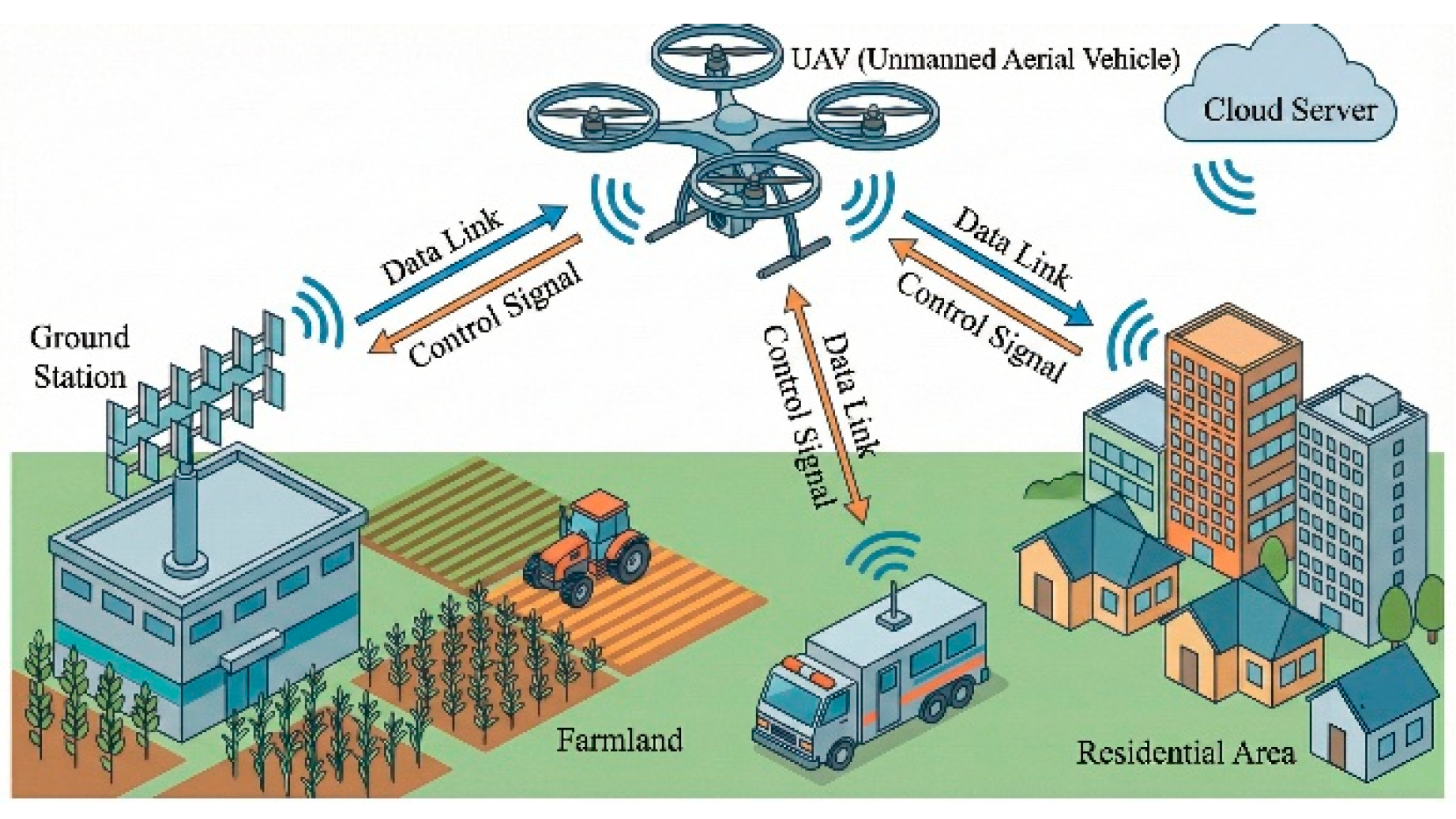
Figure 2.
Surface current distribution of periodic square metasurface for the 4x4 array, indicating in (a) mode 1, (b) mode 2, (c) mode 3, and (d) mode 4, especially, modes 3 and 4 shown orthogonal currents distribution.
Figure 2.
Surface current distribution of periodic square metasurface for the 4x4 array, indicating in (a) mode 1, (b) mode 2, (c) mode 3, and (d) mode 4, especially, modes 3 and 4 shown orthogonal currents distribution.
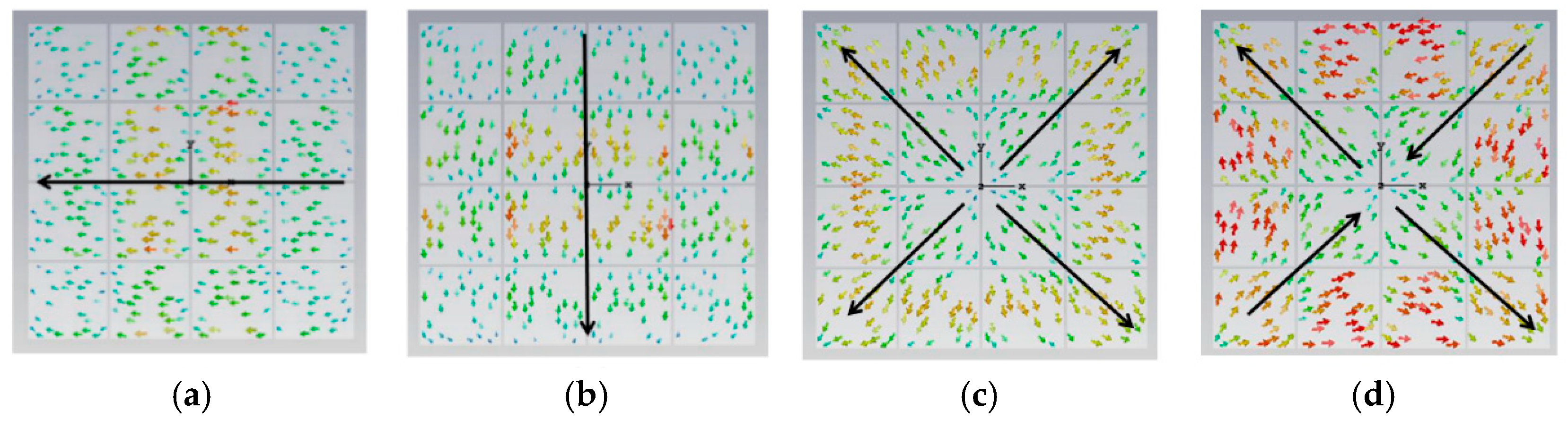
Figure 3.
Radiation pattern of a square unit metasurface for the 4x4 array, (a) mode 1, (b) mode 2, (c) mode 3, and (d) mode 4, modes 1 and 2 shown almost the same pattern, as well as modes 3 and 4.
Figure 3.
Radiation pattern of a square unit metasurface for the 4x4 array, (a) mode 1, (b) mode 2, (c) mode 3, and (d) mode 4, modes 1 and 2 shown almost the same pattern, as well as modes 3 and 4.
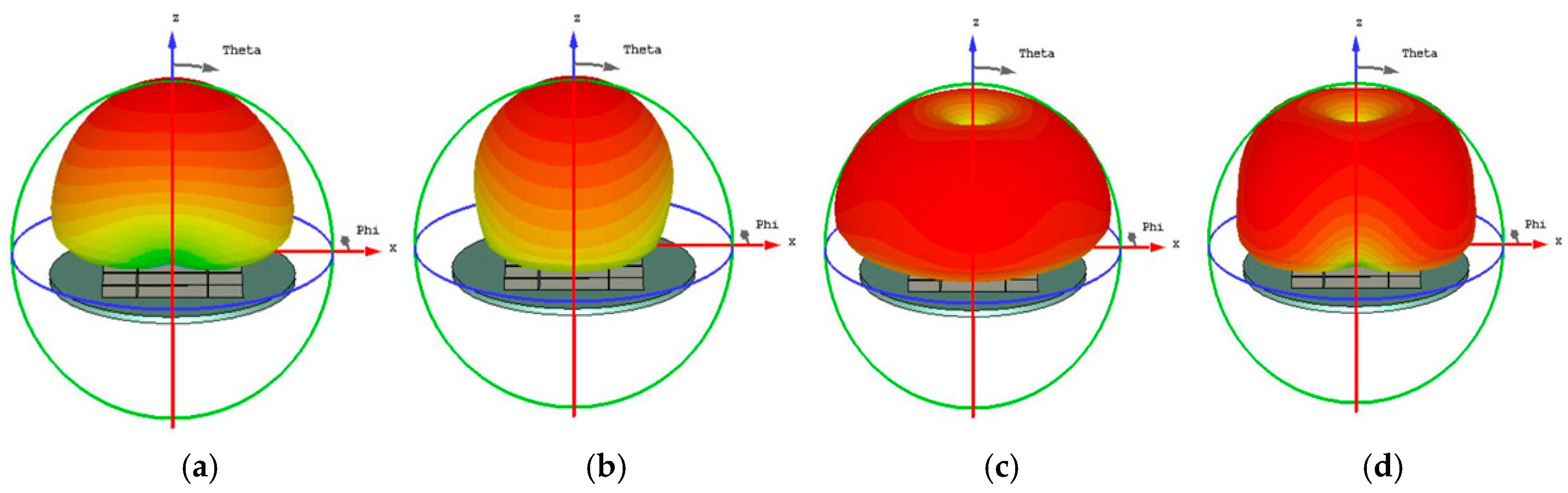
Figure 4.
The MS of 4x4 square unit metasurface, modes 1 and 2 shown almost the same MS distribution, modes 3 and 4 different, the MS peaks narrow.
Figure 4.
The MS of 4x4 square unit metasurface, modes 1 and 2 shown almost the same MS distribution, modes 3 and 4 different, the MS peaks narrow.
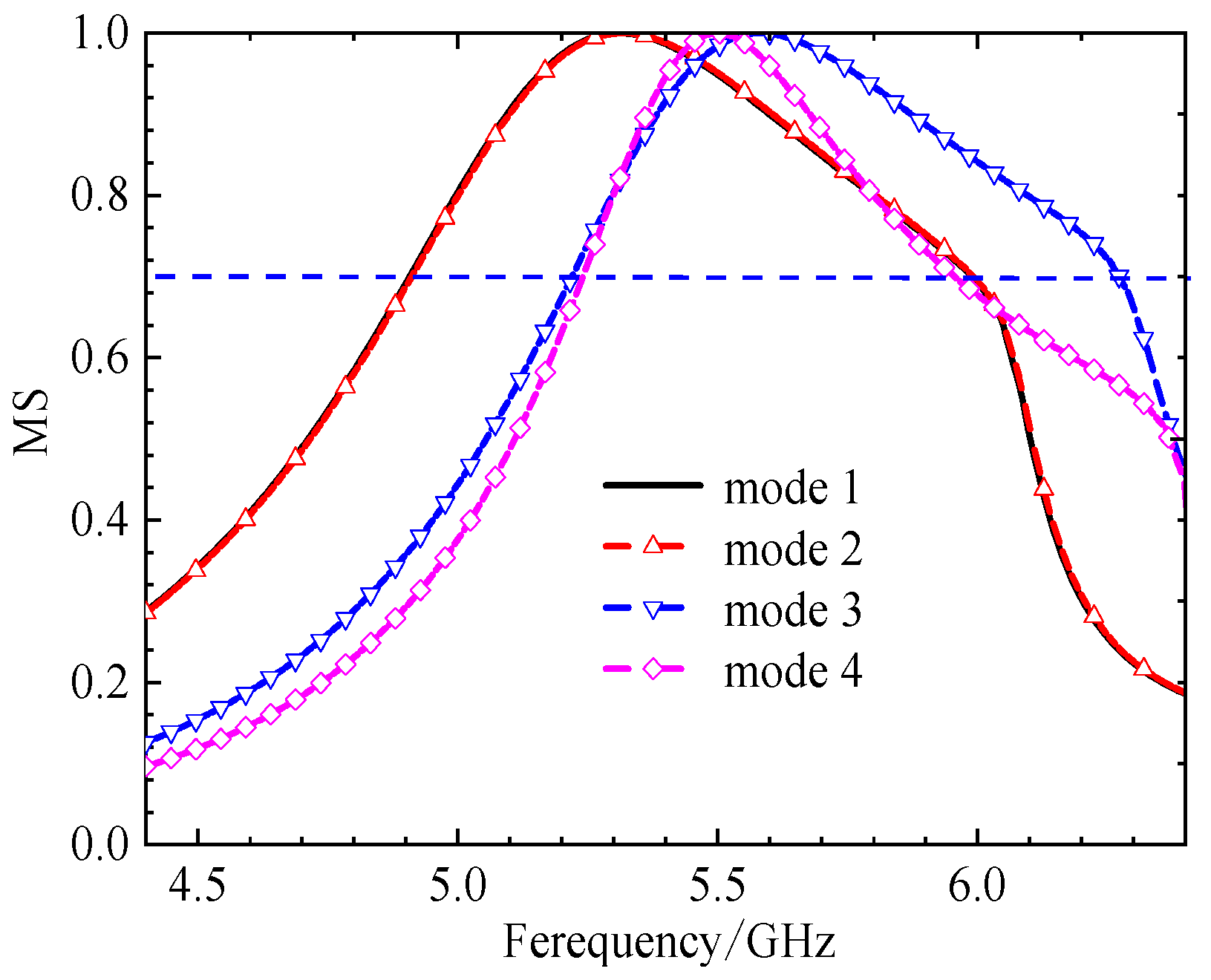
Figure 5.
Current distribution on the 4x4 metasurface while each square unit cut off a pair of opposite corners, in cases of (a) mode 1, (b) mode 2, (c) mode 3, and (d) mode 4.
Figure 5.
Current distribution on the 4x4 metasurface while each square unit cut off a pair of opposite corners, in cases of (a) mode 1, (b) mode 2, (c) mode 3, and (d) mode 4.
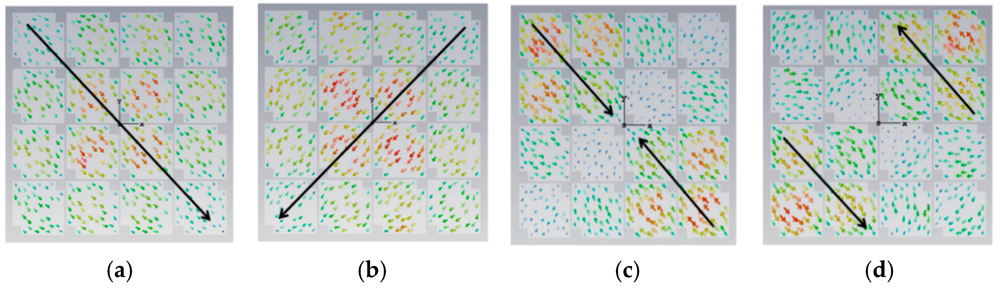
Figure 6.
Radiation pattern of 4x4 metasurface while each square unit cut off a pair of opposite corners, (a) mode 1, (b) mode 2, (c) mode 3, and (d) mode 4.
Figure 6.
Radiation pattern of 4x4 metasurface while each square unit cut off a pair of opposite corners, (a) mode 1, (b) mode 2, (c) mode 3, and (d) mode 4.
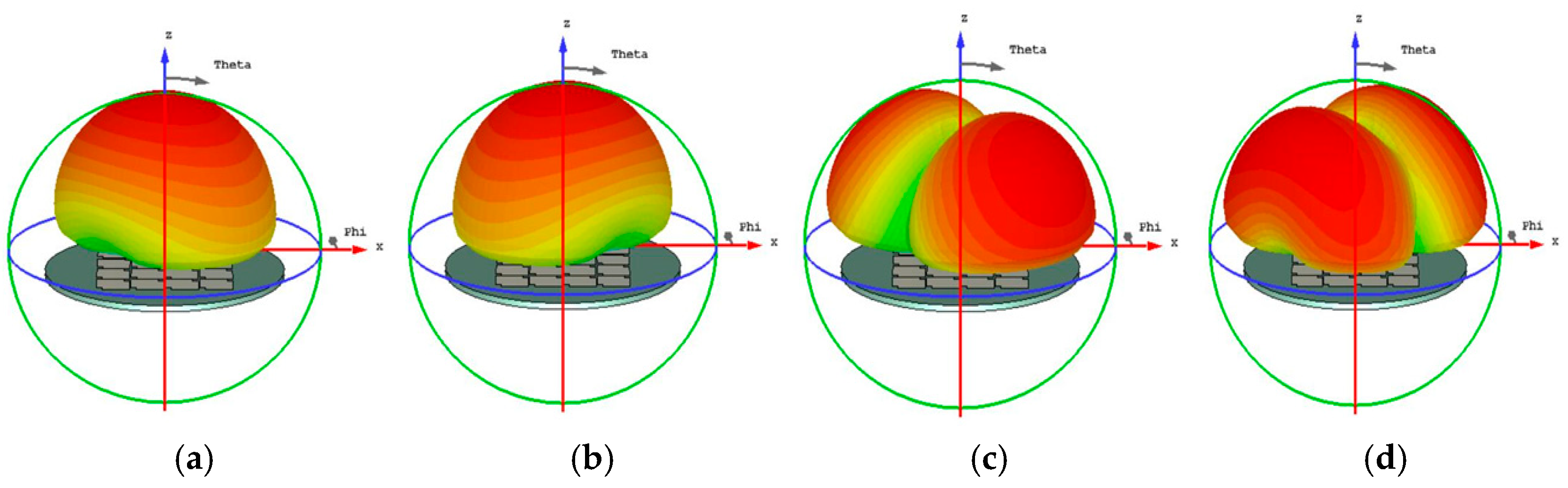
Figure 7.
The MS of 4x4 unit metasurface while each square unit cut off a pair of opposite corners, peaks moved to lower frequency.
Figure 7.
The MS of 4x4 unit metasurface while each square unit cut off a pair of opposite corners, peaks moved to lower frequency.
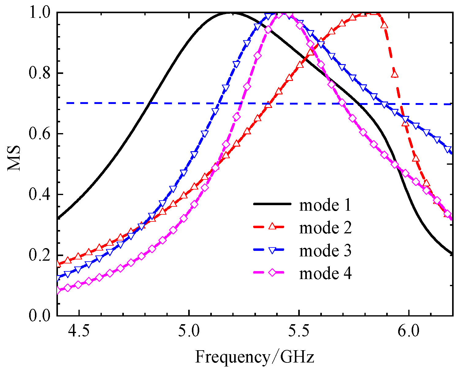
Figure 8.
Surface current distribution of each unit with two hollows (small squares), (a) mode 1, (b) mode 2, (c) mode 3, (d) mode 4.
Figure 8.
Surface current distribution of each unit with two hollows (small squares), (a) mode 1, (b) mode 2, (c) mode 3, (d) mode 4.
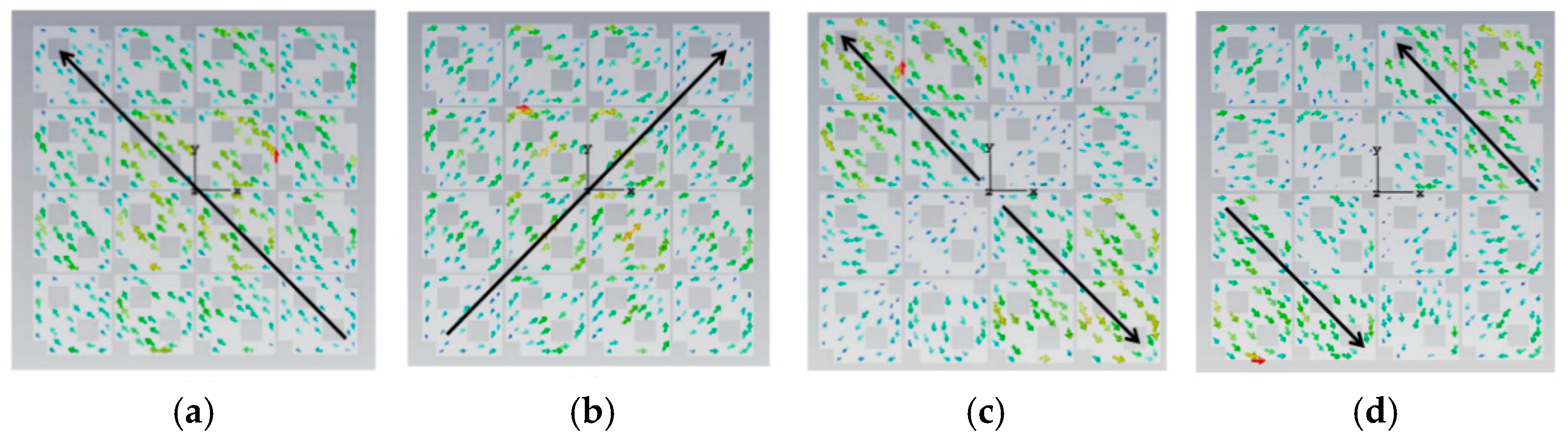
Figure 9.
Radiation pattern of each unit with two hollow (small squares), (a) mode 1, (b) mode 2, (c) mode 3, (d) mode 4.
Figure 9.
Radiation pattern of each unit with two hollow (small squares), (a) mode 1, (b) mode 2, (c) mode 3, (d) mode 4.
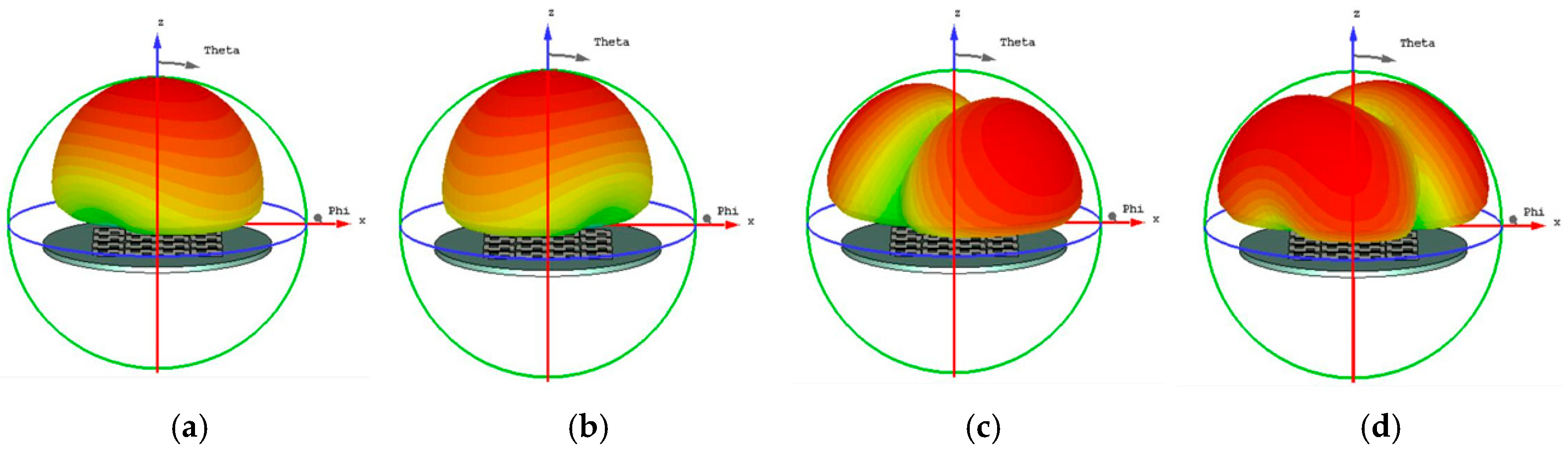
Figure 10.
The MS of each unit with two hollow small squares, peak frequency moved to lower, but too closely spaced for modes 3 and 4.
Figure 10.
The MS of each unit with two hollow small squares, peak frequency moved to lower, but too closely spaced for modes 3 and 4.
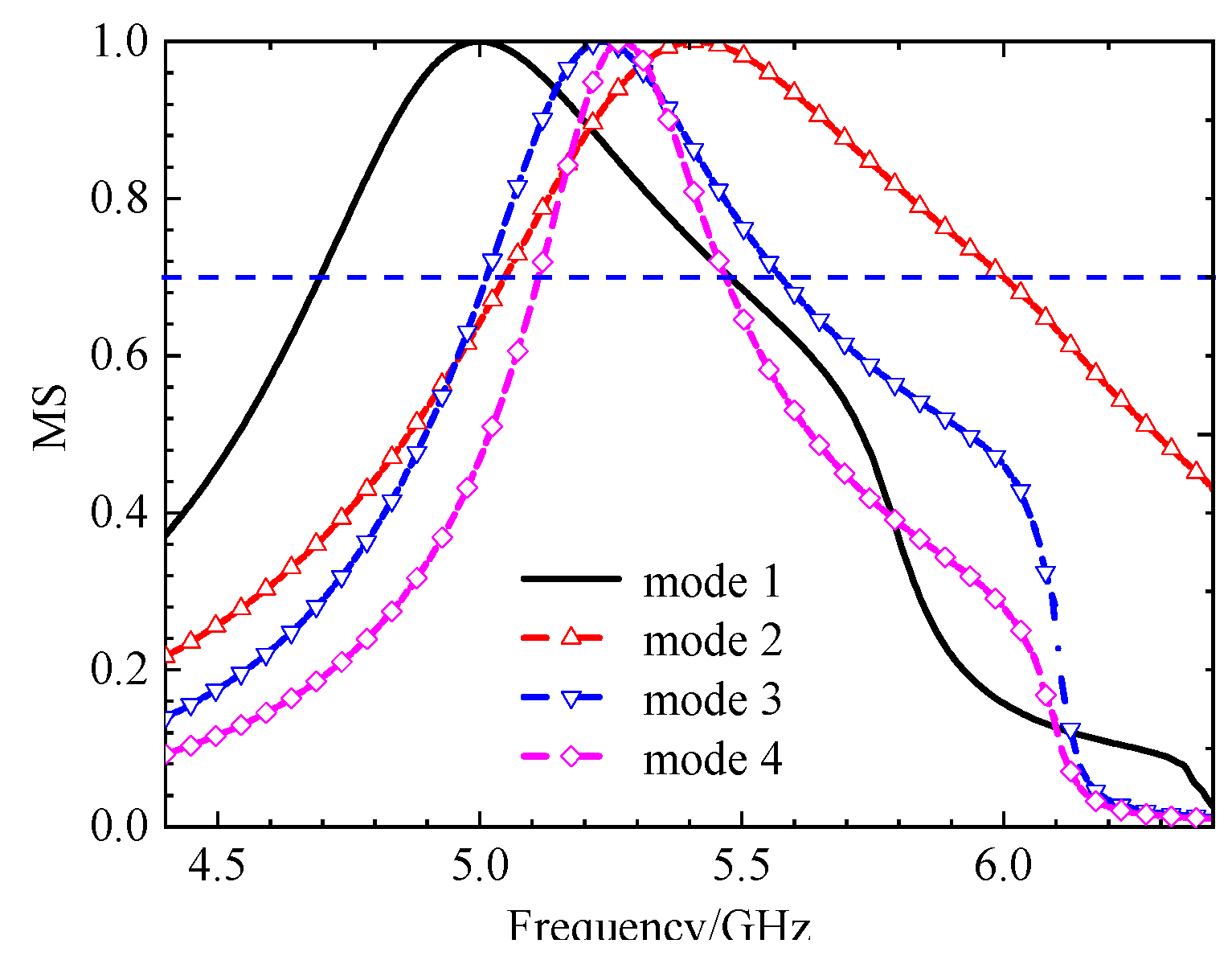
Figure 11.
Surface current distribution of small square with three hollows, (a) mode 1, (b) mode 2, (c) mode 3, and (d) mode 4.
Figure 11.
Surface current distribution of small square with three hollows, (a) mode 1, (b) mode 2, (c) mode 3, and (d) mode 4.
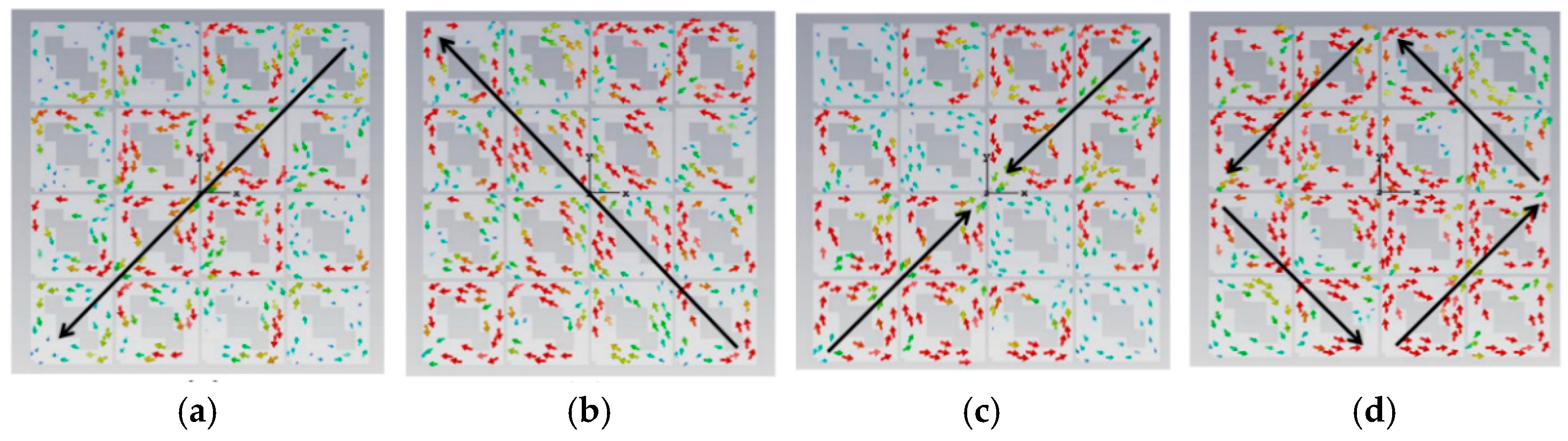
Figure 12.
Radiation pattern of 4x4 metasurfaces, each square unit with three hollow small squares, (a) mode 1, (b) mode 2, (c) mode 3, and (d) mode 4.
Figure 12.
Radiation pattern of 4x4 metasurfaces, each square unit with three hollow small squares, (a) mode 1, (b) mode 2, (c) mode 3, and (d) mode 4.
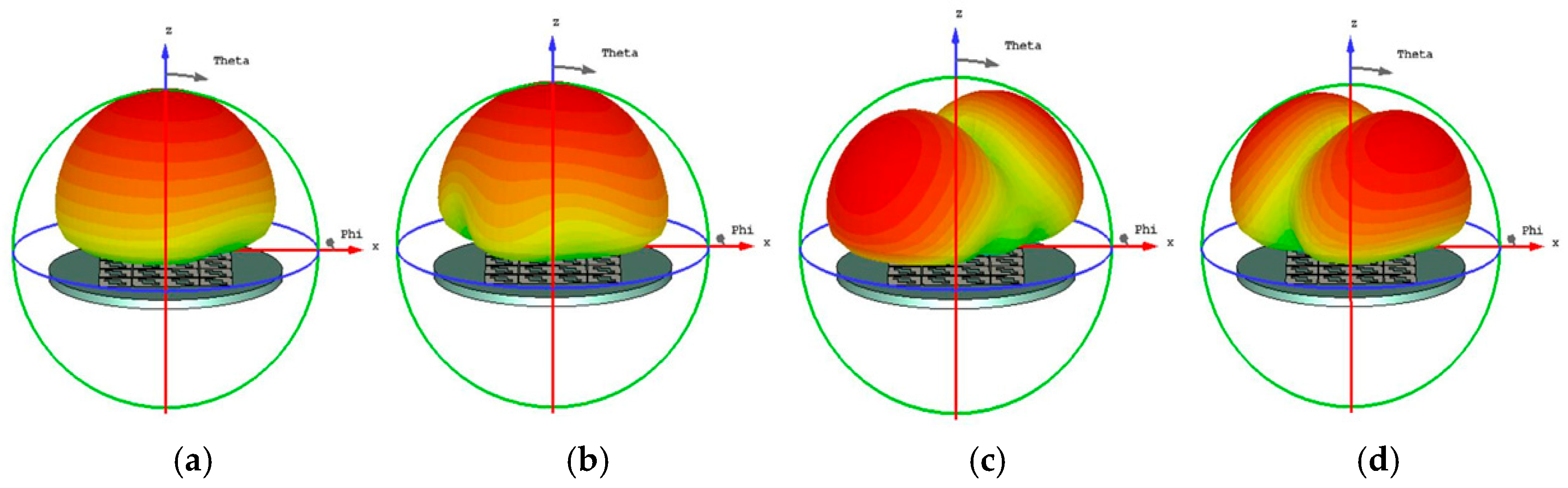
Figure 13.
The MS of 4x4 metasurfaces, each unit with three hollow small squares, the peak frequency with space enough.
Figure 13.
The MS of 4x4 metasurfaces, each unit with three hollow small squares, the peak frequency with space enough.
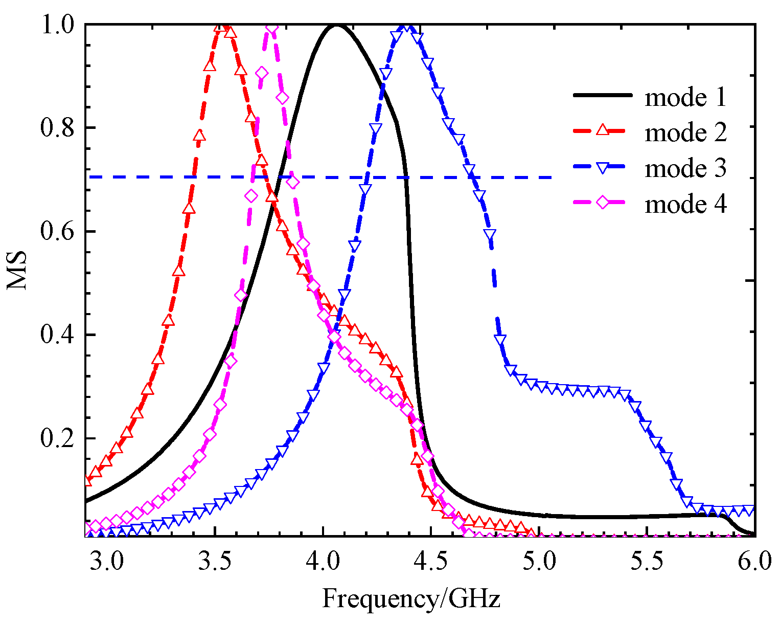
Figure 14.
Principle diagram of achieving polarization reconfigurable metasurface, (a) initial Position, (b) rotate 45°, and (c) rotate 90°.
Figure 14.
Principle diagram of achieving polarization reconfigurable metasurface, (a) initial Position, (b) rotate 45°, and (c) rotate 90°.
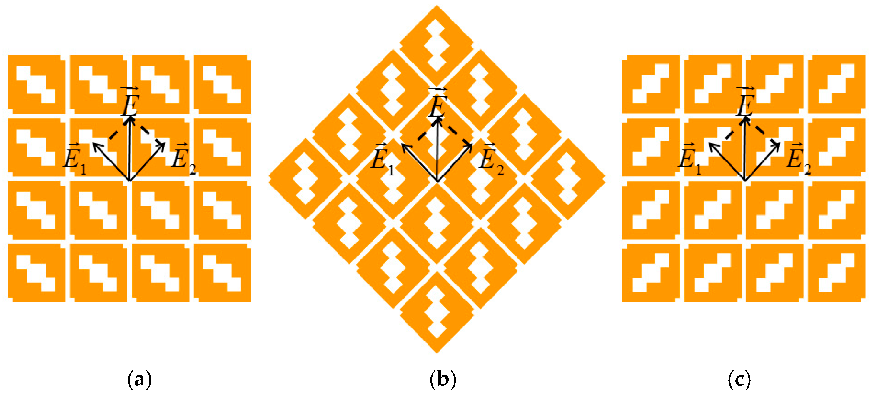
Figure 15.
Characteristic angle (CA) of metasurfaces with three hollow small squares.
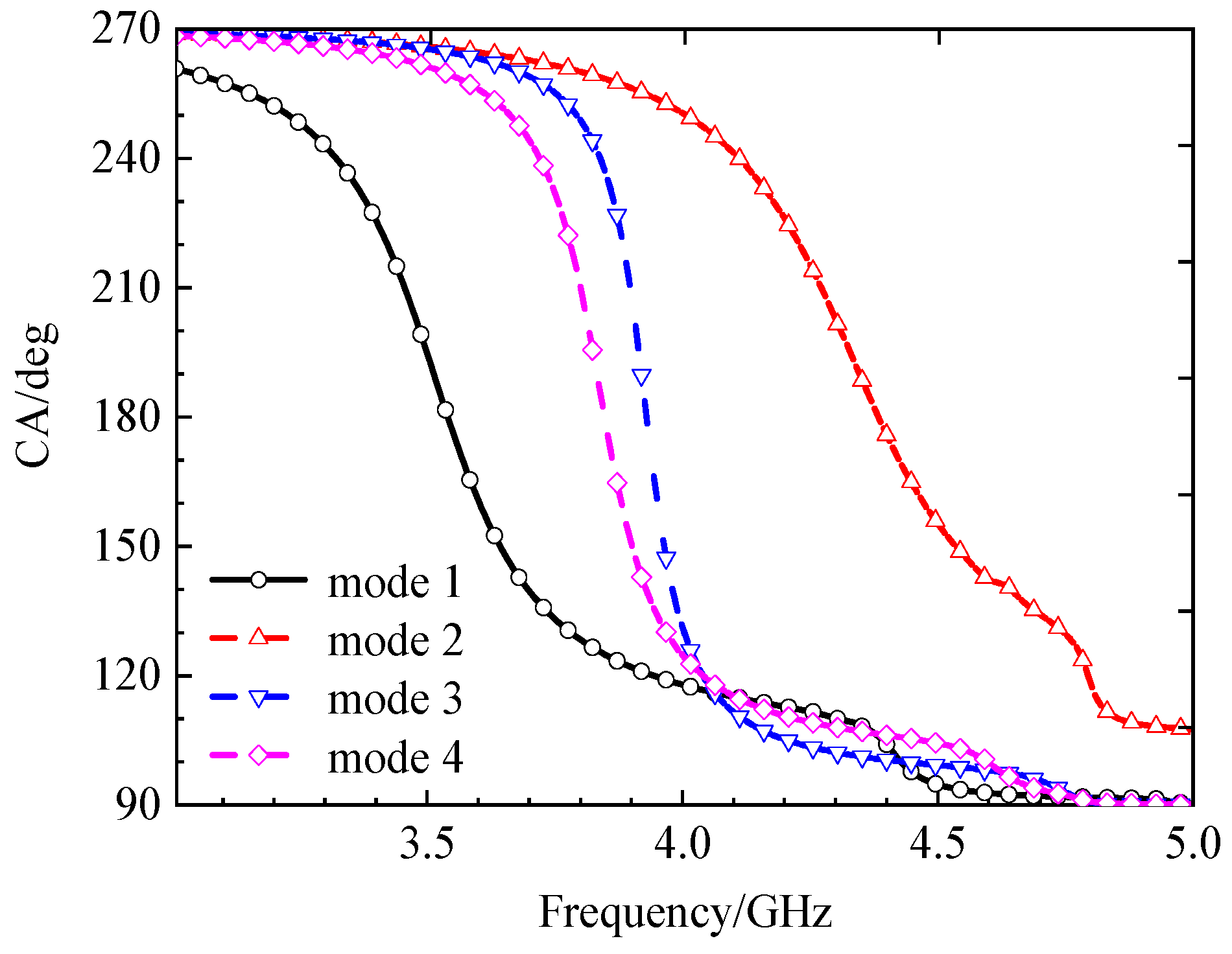
Figure 16.
Final designed Antenna Structure, metasurfaces with three hollow small squares, (a) top and side view, (b) bottom view (feed & ground).
Figure 16.
Final designed Antenna Structure, metasurfaces with three hollow small squares, (a) top and side view, (b) bottom view (feed & ground).
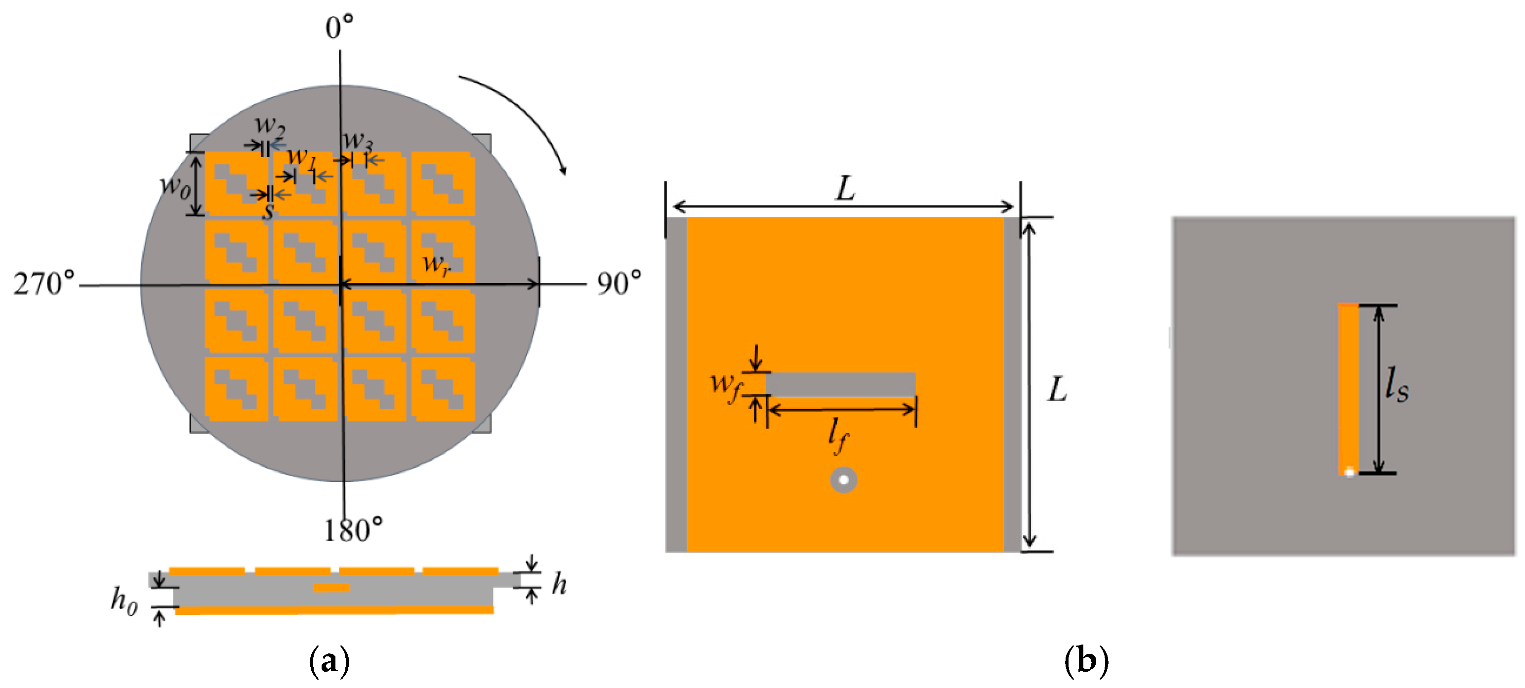
Figure 17.
Simulation results of |S11| for different thicknesses of circular dielectric substrates h, square dielectric substrates h0, strip patch length ls and gap width wf, (a)parameters h, (b) parameters h0, (c) parameters ls, and (d) parameters wf.
Figure 17.
Simulation results of |S11| for different thicknesses of circular dielectric substrates h, square dielectric substrates h0, strip patch length ls and gap width wf, (a)parameters h, (b) parameters h0, (c) parameters ls, and (d) parameters wf.
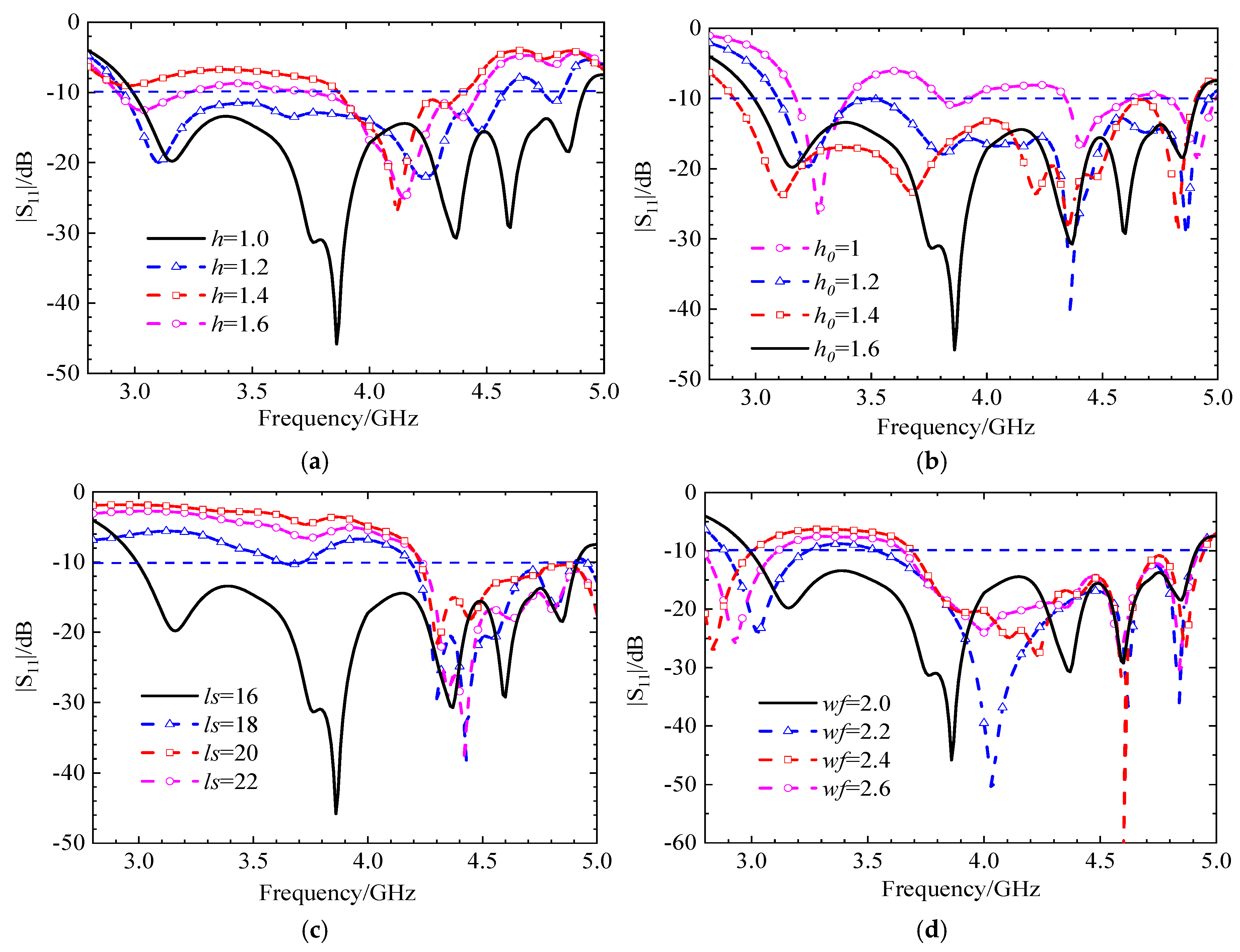
Figure 18.
Simulation diagram of LHCP and LHCP, (a) phi=0°, (b) phi=90°.
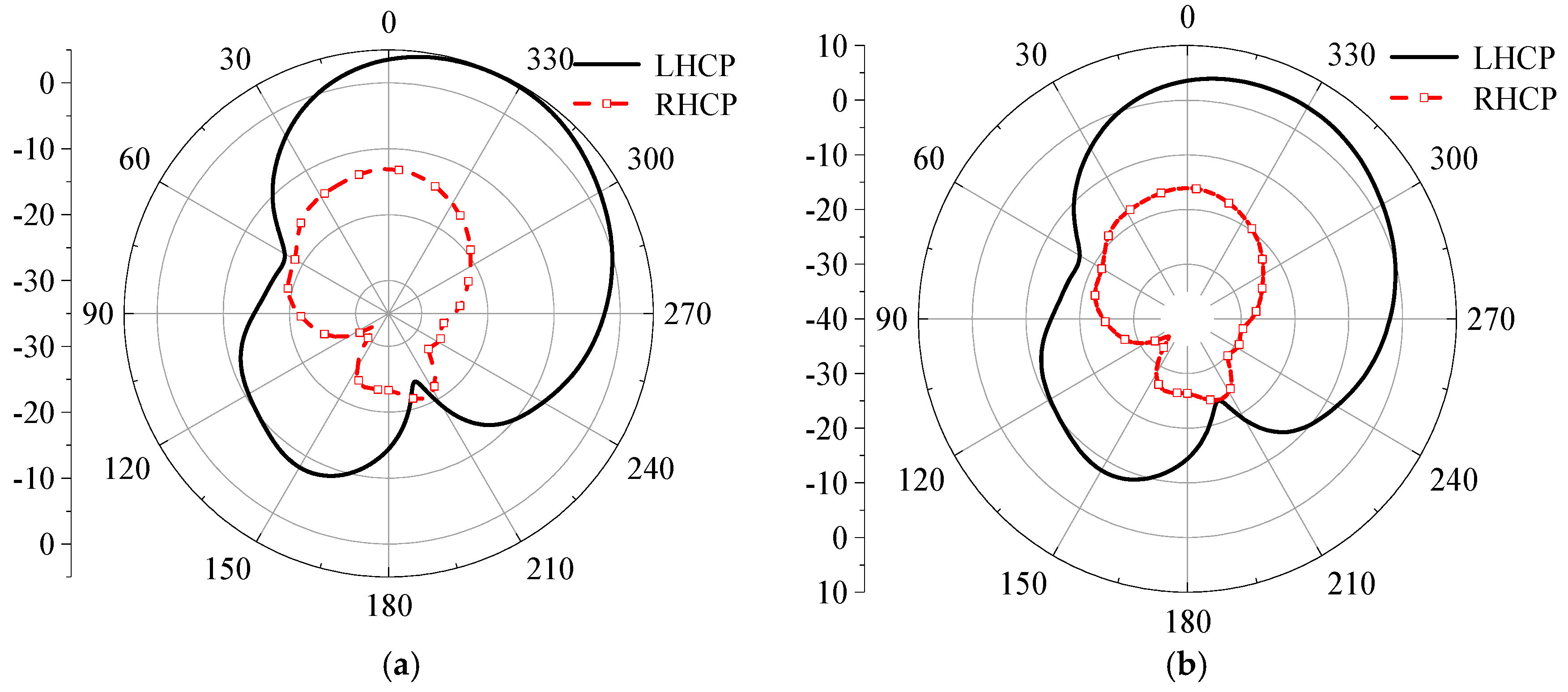
Figure 19.
Simulation results of |S11| for different thicknesses of circular dielectric substrates h, strip patch length ls, gap length lf and gap width wf, (a)parameters h, (b) parameters ls, (c) parameters lf, and (d) parameters wf.
Figure 19.
Simulation results of |S11| for different thicknesses of circular dielectric substrates h, strip patch length ls, gap length lf and gap width wf, (a)parameters h, (b) parameters ls, (c) parameters lf, and (d) parameters wf.
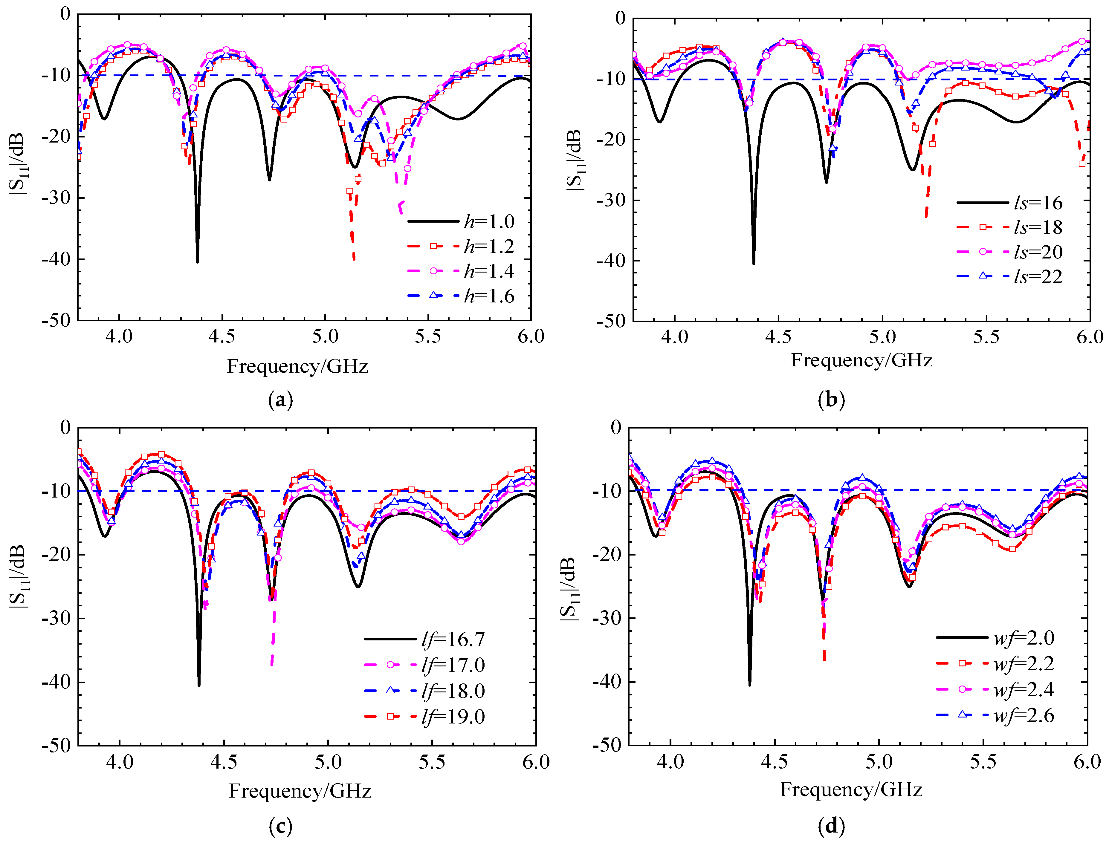
Figure 20.
Simulation diagram of main-polarization (MP) and cross-polarization (CP), (a) phi=0°, (b) phi=90°.
Figure 20.
Simulation diagram of main-polarization (MP) and cross-polarization (CP), (a) phi=0°, (b) phi=90°.
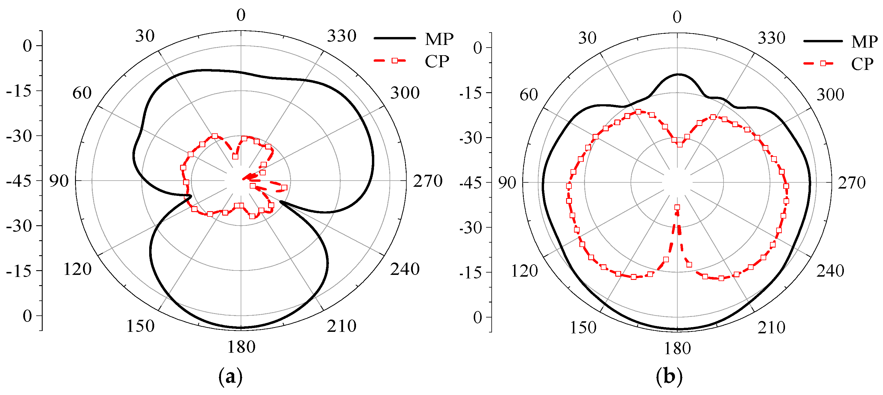
Figure 21.
Simulation results of |S11| for different thicknesses of circular dielectric substrates h, square dielectric substrates h0, gap length lf and gap width wf, (a) parameters h, (b) parameters h0, (c) parameters lf, and (d) parameters wf.
Figure 21.
Simulation results of |S11| for different thicknesses of circular dielectric substrates h, square dielectric substrates h0, gap length lf and gap width wf, (a) parameters h, (b) parameters h0, (c) parameters lf, and (d) parameters wf.
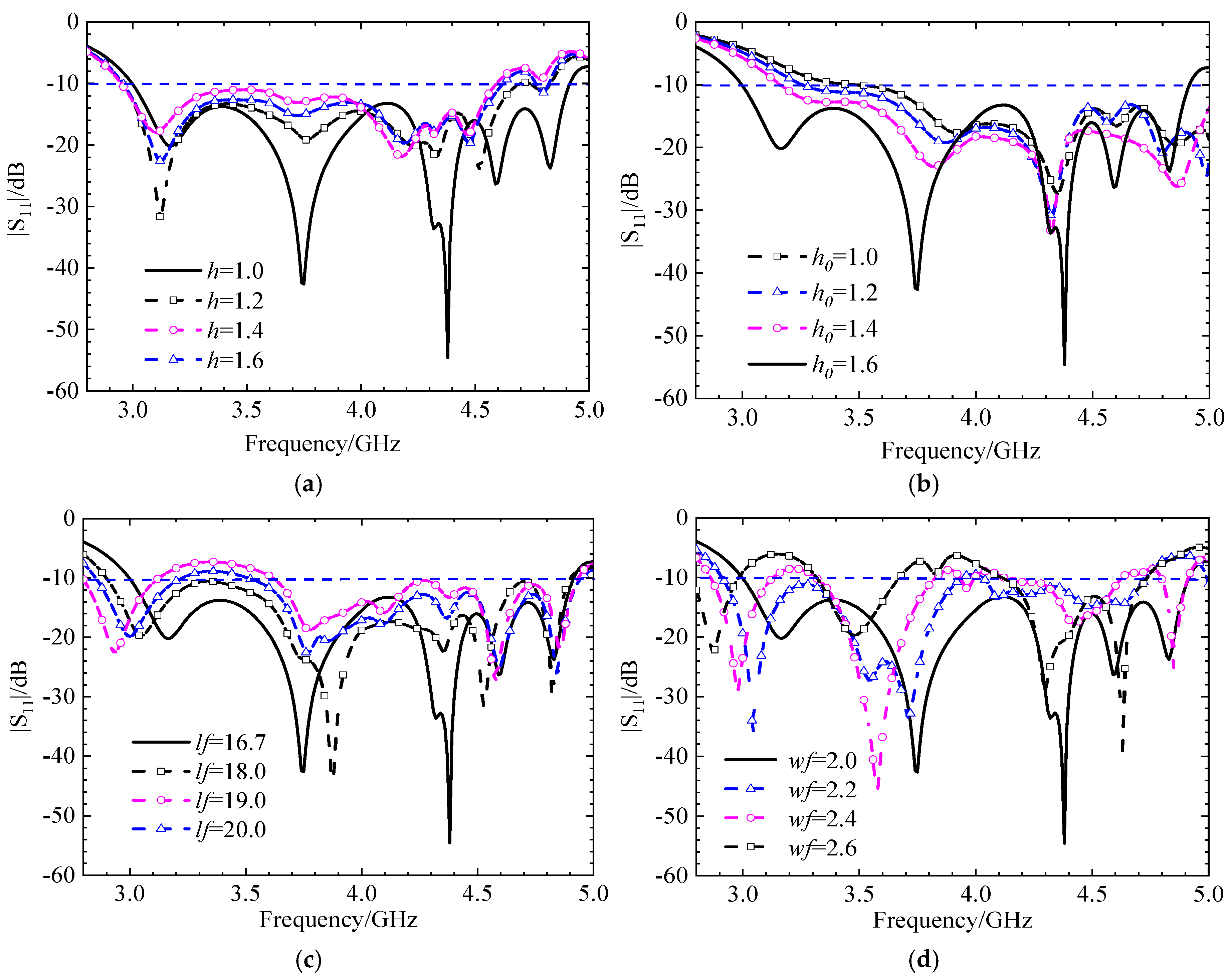
Figure 22.
Simulation diagram of LHCP and RHCP, (a) phi=0°, (b) phi=90°.
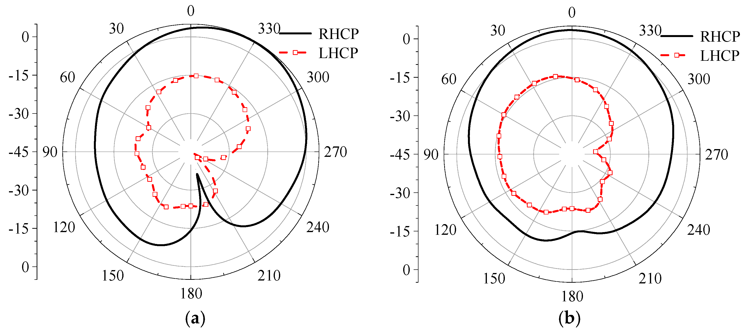
Figure 23.
Physical and test images of antennas, (a) physical image of antenna, (b) test diagram of antenna connection to vector network, and (c) test diagram of line in microwave anechoic chamber.
Figure 23.
Physical and test images of antennas, (a) physical image of antenna, (b) test diagram of antenna connection to vector network, and (c) test diagram of line in microwave anechoic chamber.
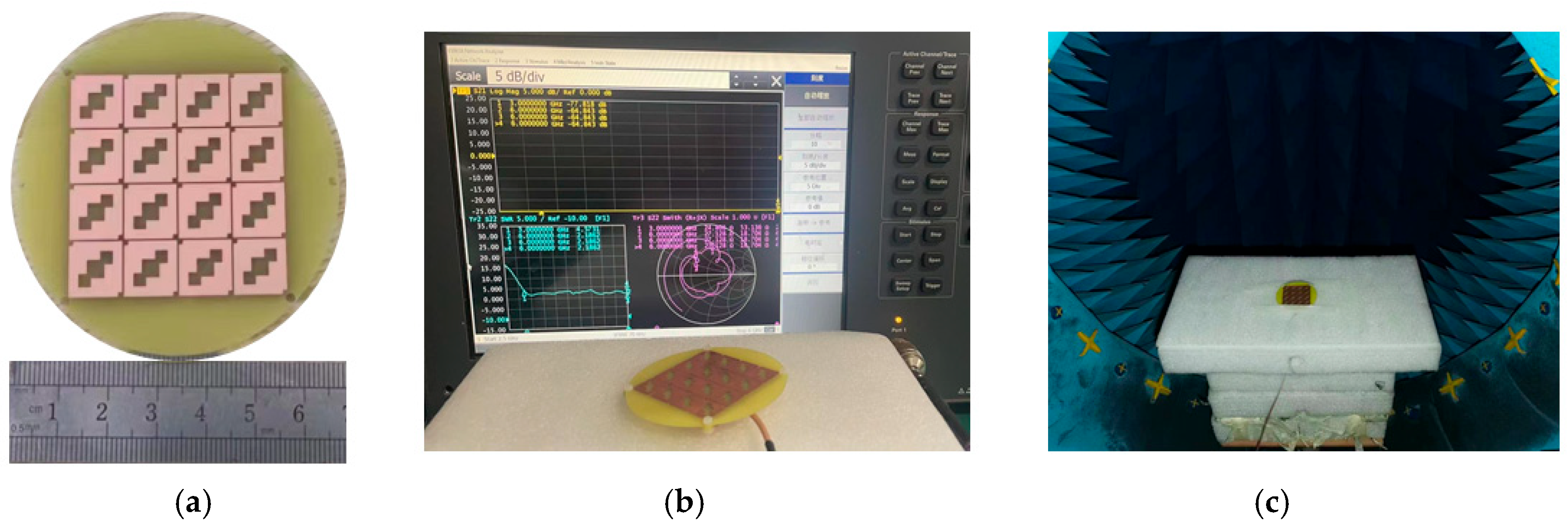
Figure 24.
Comparison between simulation (Simu.) and measurement (Measu.) of |S11| antenna at initial position.
Figure 24.
Comparison between simulation (Simu.) and measurement (Measu.) of |S11| antenna at initial position.
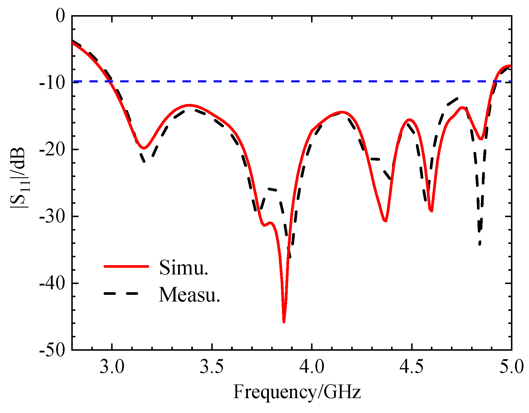
Figure 25.
Comparison between simulation and testing of gain and axial bandwidth at initial position, (a) gain chart, (b) axis ratio (AR) bandwidth graph.
Figure 25.
Comparison between simulation and testing of gain and axial bandwidth at initial position, (a) gain chart, (b) axis ratio (AR) bandwidth graph.
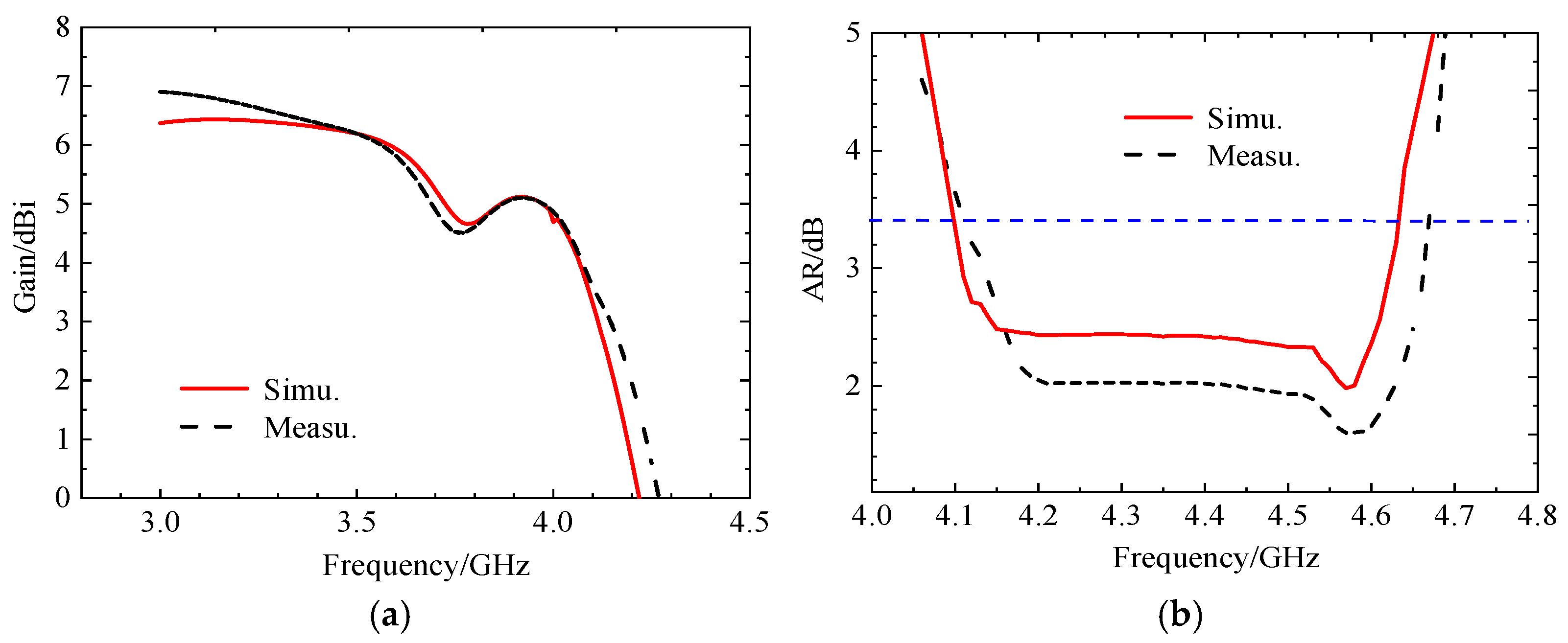
Figure 26.
Simulation and measurement of radiation pattern, antenna at initial position, (a) 3.85 GHz, (b) 4.37 GHz.
Figure 26.
Simulation and measurement of radiation pattern, antenna at initial position, (a) 3.85 GHz, (b) 4.37 GHz.
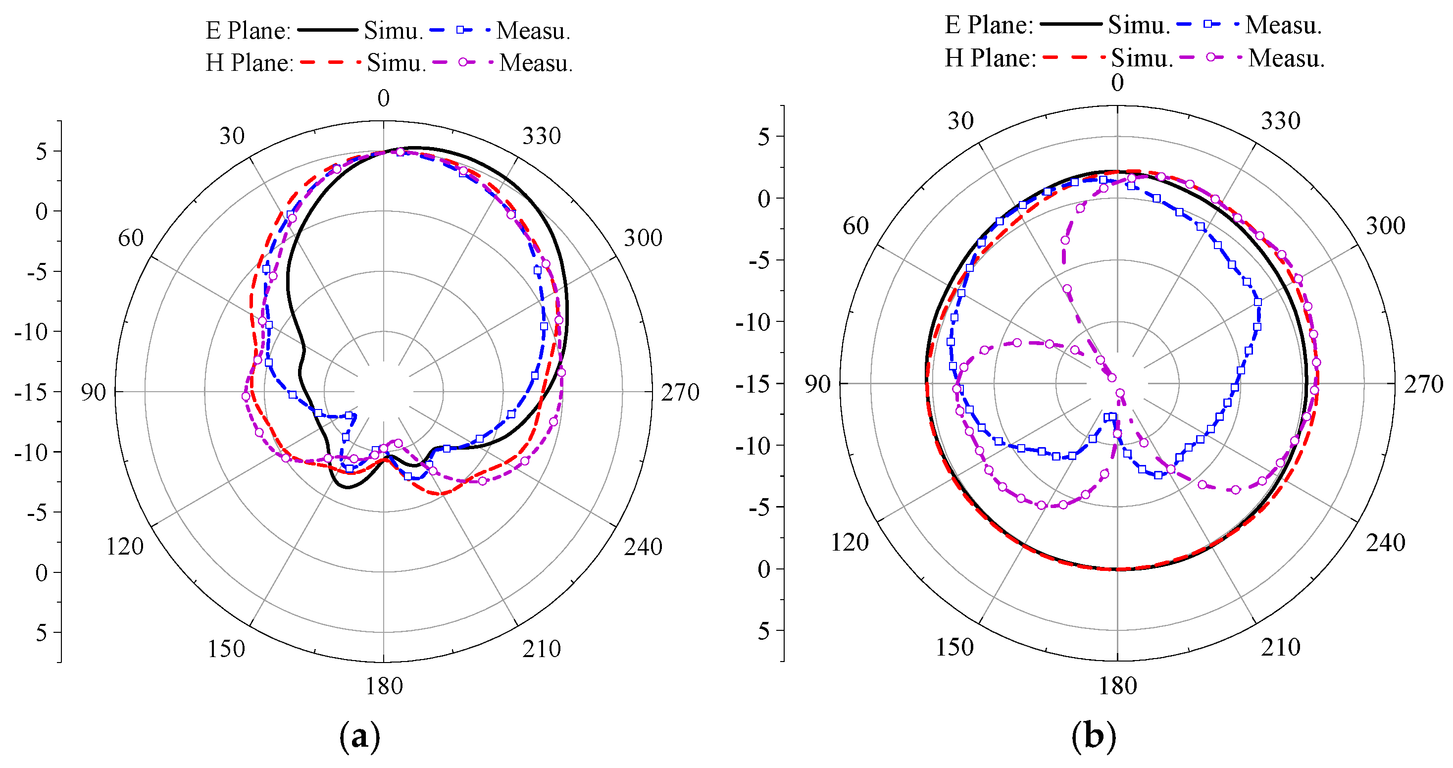
Figure 27.
Simulation and measurement of the LHCP and RHCP at initial position, (a) phi = 0°, (b) phi = 90°.
Figure 27.
Simulation and measurement of the LHCP and RHCP at initial position, (a) phi = 0°, (b) phi = 90°.
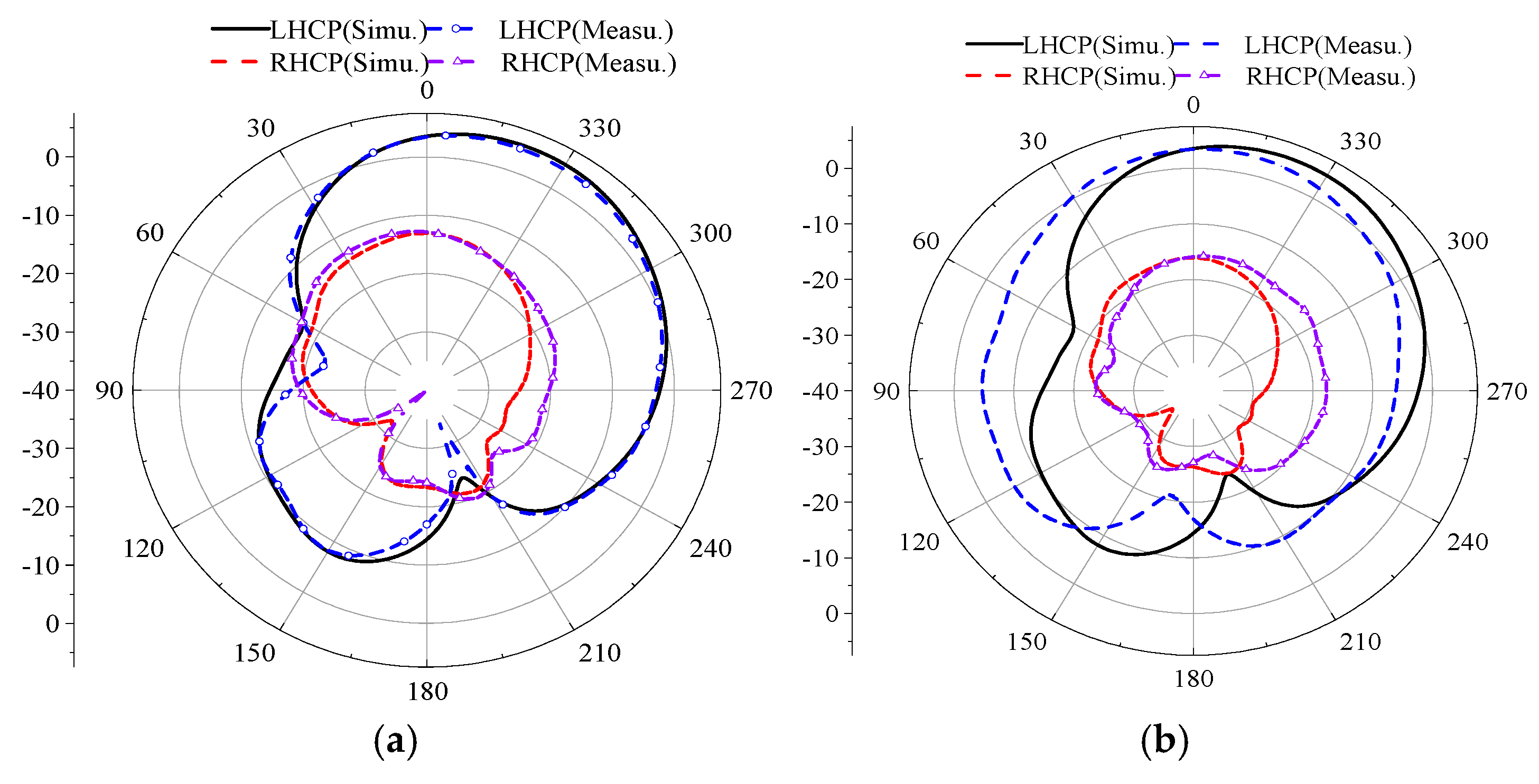
Figure 28.
Simulation and measurement of antenna radiation patterns when rotating 90°, (a) 3.85 GHz, (b) 4.37 GHz.
Figure 28.
Simulation and measurement of antenna radiation patterns when rotating 90°, (a) 3.85 GHz, (b) 4.37 GHz.
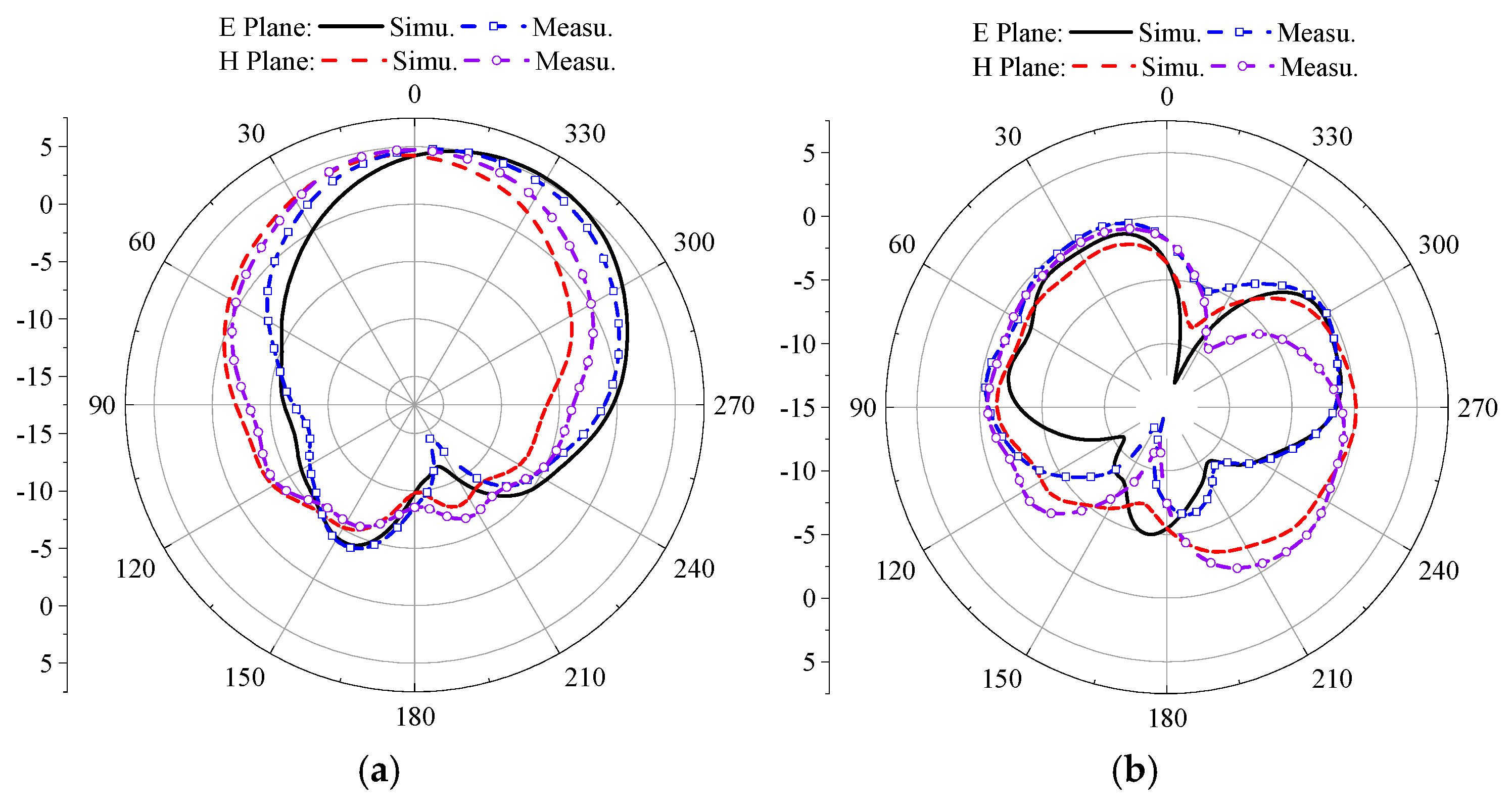
Figure 29.
Simulation and test comparison of left-handed circular polarization and right-handed circular polarization at 90 ° rotation (a) phi = 0°, (b) phi = 90° E plane.
Figure 29.
Simulation and test comparison of left-handed circular polarization and right-handed circular polarization at 90 ° rotation (a) phi = 0°, (b) phi = 90° E plane.
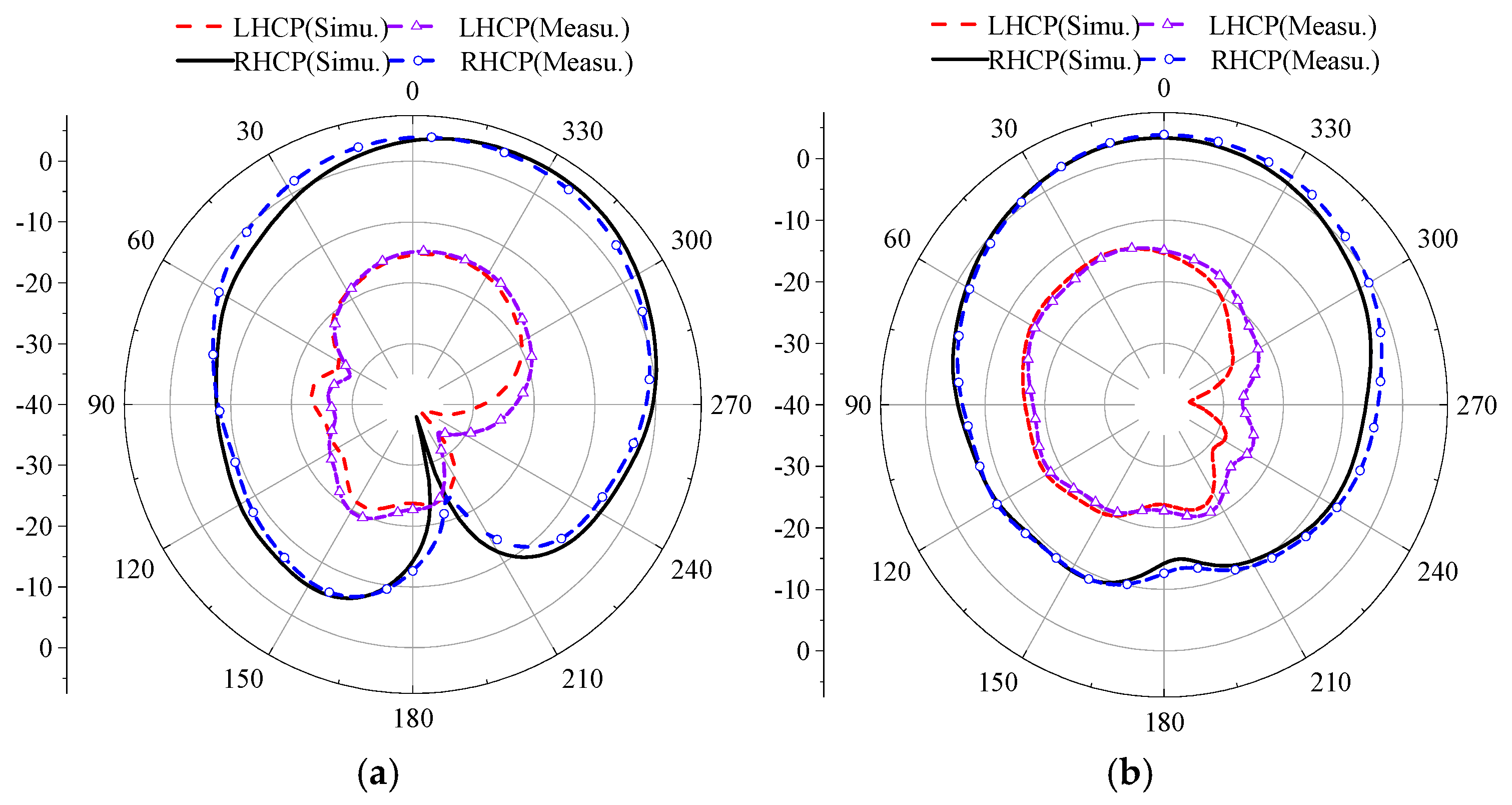

Table 1.
Final Size of Designed Antenna.
| Dimension | w0 | w1 | w2 | w3 | wr | wf |
| Size (mm) | 11 | 3.68 | 2.5 | 2.5 | 35 | 2 |
| Dimension | L | lf | ls | h0 | h | s |
| Size (mm) | 50 | 16.7 | 16 | 1.6 | 1 | 1 |
Table 2.
Summary of Antenna Performance.
| Polarization State | Parameter | Simulation | Measurement |
| LHCP (0°) | Impedance BW | 48.17% (3.01–4.92 GHz) | 47.0% (3.05–4.89 GHz) |
| 3-dB AR BW | 9.75% (4.12–4.64 GHz) | 10.3% (4.15–4.60 GHz) | |
| Avg. Gain | 5.9 dBi | 5.7 dBi | |
| LP (45°) | Impedance BW | 32.68% (4.30–5.98 GHz) | 29.9% (4.33–5.85 GHz) |
| XPD (Co/Cross-pol) | >23 dB | >23 dB | |
| Avg. Gain | 5.3 dBi | 5.1 dBi | |
| RHCP (90°) | Impedance BW | 48.29% (3.00–4.91 GHz) | 48.5% (2.98–4.88 GHz) |
| 3-dB AR BW | 9.98% (3.46–3.82 GHz) | 10.1% (3.42–3.78 GHz) | |
| Avg. Gain | 6.1 dBi | 6.0 dBi |
Disclaimer/Publisher’s Note: The statements, opinions and data contained in all publications are solely those of the individual author(s) and contributor(s) and not of MDPI and/or the editor(s). MDPI and/or the editor(s) disclaim responsibility for any injury to people or property resulting from any ideas, methods, instructions or products referred to in the content. |
© 2026 by the authors. Licensee MDPI, Basel, Switzerland. This article is an open access article distributed under the terms and conditions of the Creative Commons Attribution (CC BY) license.
Copyright: This open access article is published under a Creative Commons CC BY 4.0 license, which permit the free download, distribution, and reuse, provided that the author and preprint are cited in any reuse.


