
Submitted:
08 January 2026
Posted:
09 January 2026
You are already at the latest version
Abstract
Motion artifacts corruptwearable ECG signals and generate false alarms of arrhythmias, limiting the clinical adoption of continuous cardiacmonitoring. We present a dual-streamdeep learning framework formotionrobust binary arrhythmia classification throughmulti-modal sensor fusion andmulti-SNR training. ResNet-18 processes ECG spectrograms,while CNN-BiLSTMencodes accelerometermotion patterns; attention-gated fusion with gate diversity regularization adaptively weightsmodalities based on signal reliability. Training in MIT-BIHdata augmented at three noise levels (24, 12, 6 dB) enables noise-invariant learningwith successful generalization to unseen conditions. The framework achieves 99.5%accuracy under clean signals, gracefully degrading to 88.2%at extreme noise (-6 dB SNR)—a 46%improvement over trainingwith single-SNR. The high gate diversity (σ > 0.37) confirms adaptive context-dependent fusion. With 0.09% false positive rate and real-time processing (238 beats/second), the systemprovides practical continuous arrhythmia screening, establishing the foundation for hierarchical monitoring systems where binary screening activates detailed multi-class diagnosis.
Keywords:
arrhythmia detection
; motion artifacts
; sensor fusion
; wearable ECG
; deep learning
; false alarm reduction
; MIT-BIH
; accelerometer
1. Introduction
1.1. Clinical Problem: False Alarms in Wearable Cardiac Monitoring
Cardiac arrhythmias cause approximately 60,000 cardiac arrests per year in Canada, with atrial fibrillation (AF) affecting more than 33 million people around the world and increasing the risk of stroke five times [1]. Wearable electrocardiogram (ECG) monitors offer unprecedented opportunities for continuous arrhythmia surveillance in ambulatory settings, but a critical limitation undermines their clinical adoption: motion artifacts generate false alarms that overwhelm healthcare providers and undermine patient trust [2].
Studies of intensive care unit (ICU) alarms reveal that 85-99% of arrhythmia alerts are false positives, primarily caused by patient movement, electrode displacement, and electromyographic interference [3]. In ambulatory monitoring, where patients engage in unrestricted daily activities, motion artifact contamination intensifies dramatically. A patient walking briskly may trigger dozens of spurious ventricular tachycardia alarms; running induces artifact patterns resembling atrial fibrillation; even reaching for objects generates transient signal distortions flagged as premature ventricular contractions.
This false alarm epidemic has severe consequences. Healthcare providers develop "alarm fatigue," becoming desensitized to alerts and potentially missing real life-threatening events [5]. Patients lose confidence in monitoring systems that cry wolf repeatedly, reducing compliance with prescribed monitoring regimens. The fundamental challenge is clear: how can we reliably distinguish true cardiac arrhythmia from benign signal distortions caused by physical activity?
1.2. Limitations of Existing Approaches
Traditional ECG processing algorithms employ signal quality indices (SQI) that attempt to identify corrupted segments and suppress analysis during poor-quality intervals [6]. Although conceptually sound, SQI-based approaches face an inherent dilemma: aggressive quality thresholds reduce false positives, but risk missing genuine arrhythmia occurring during movement; lenient thresholds maintain sensitivity, but allow false alarms to proliferate.
Advanced motion artifact rejection techniques including adaptive filtering [9], independent component analysis (ICA), and wavelet denoising [10] operate purely in the signal processing domain without utilizing contextual information about patient activity. These methods attempt to extract the cardiac signal from corrupted recordings, but cannot distinguish whether detected abnormalities represent true pathology or residual artifacts.
Recent deep learning approaches for arrhythmia detection achieve remarkable accuracy in benchmark databases with clean signals [3,11], yet performance degrades catastrophically when evaluated in motion-corrupted data. Convolutional neural networks trained on curated datasets learn to recognize canonical arrhythmia patterns but fail when faced with morphological distortions and rhythm irregularities induced by motion artifacts.
1.3. Multi-Modal Sensor Fusion Solution
We address motion artifact challenges through attention-gated multi-modal fusion, integrating ECG spectrogram analysis with tri-axial accelerometer measurements that quantify patient movement. The key insight is that correlated sensor information such as cardiac electrical activity and body motion enables robust arrhythmia detection under varying signal quality conditions. By learning adaptive sensor weighting, the system maintains high accuracy in clean and motion-corrupted scenarios without requiring explicit noise classification or hand-crafted fusion rules.
Our framework processes ECG and accelerometer data through specialized parallel encoders that extract complementary representations: ECG spectrograms capture time-frequency cardiac dynamics through ResNet-18 convolutional networks (512-dimensional features), while accelerometer time-series are processed through CNN-BiLSTM networks that characterize motion patterns and temporal dependencies (128-dimensional features). Rather than fixed fusion weights or rule-based combination, we employ learnable attention gates that dynamically balance the contribution of each modality based on the reliability and discriminative power of the extracted features for each individual sample.
Attention-gated fusion mechanism: The fusion module computes scalar attention weights and through small multilayer perceptrons applied to batch-normalized features. These gates modulate the importance of each stream before concatenation:
Gates are initialized to produce balanced fusion () at the beginning of the training, then adapt through backpropagation to learn optimal sensor weighting. Critically, we enforce gate diversity through explicit regularization () that penalizes uniform gate values, preventing the common failure mode where gates collapse to constants and effectively disable adaptive behavior.
Learned fusion strategy: During training in multi-SNR augmented data (24, 12, 6 dB), the network learns an ECG-dominant fusion policy with and on average. However, these gates exhibit substantial variation between samples (), indicating context-dependent adaptation rather than fixed weighting. The accelerometer serves as a complementary information source that aids in classification when the ECG morphology alone is ambiguous due to noise corruption, while the ECG stream maintains primary diagnostic responsibility given its superior discriminative power for cardiac rhythm abnormalities.
1.4. Paper Organization
The paper is structured as follows: Section 2 surveys existing approaches to motion artifact mitigation, arrhythmia classification algorithms, and multi-modal fusion techniques in wearable health monitoring. Section 3 establishes the mathematical foundation, detailing the computation of the ECG spectrogram, the extraction of accelerometer characteristics, and the fusion mechanism with attention-gated fusion with loss of gate diversity. Section 4 describes the dual-stream deep neural network architecture, including ResNet-18 for ECG analysis, CNN-BiLSTM for motion characterization, and the fusion classifier. Section 5 presents the data set (MIT-BIH Arrhythmia Database), the multi-SNR augmentation protocol using NST noise, and the evaluation methodology. Section 6 reports comprehensive performance metrics for noise conditions, confusion matrix analysis, and attention gate statistics. Section 7 analyzes the multi-SNR training strategy, clinical deployment implications, and the binary-first hierarchical monitoring paradigm. Section 8 summarizes the contributions and acknowledges the limitations.
2. Related Work
2.1. Motion Artifact Rejection in ECG
Motion artifacts have plagued ambulatory ECG monitoring since its inception. Classical approaches employ adaptive filtering that estimates the artifact components using reference noise measurements and then subtracts the estimates from the corrupted ECG [9]. However, acquiring clean reference noise signals without cardiac content proves challenging in practice, limiting effectiveness.
Wavelet-based methods decompose ECG signals into multi-resolution sub-bands, applying thresholding to suppress artifact-dominated coefficients while preserving cardiac information [6,10]. These techniques excel at removing baseline wander and high-frequency muscle noise, but struggle with motion artifacts that exhibit spectral overlap with cardiac signals.
Independent Component Analysis (ICA) uses statistical independence to separate mixed source signals, decomposing multi-lead ECG recordings into independent components that represent cardiac activity versus artifacts [23]. While powerful for multi-lead systems, single-lead wearable devices cannot provide the multiple observations required for effective blind source separation.
Template matching and morphological filtering attempt to identify and remove artifact segments by comparing beat morphology against learned templates [24]. These methods implicitly assume artifacts produce morphologically distinct patterns, an assumption violated when artifacts subtly distort rather than grossly corrupt cardiac waveforms.
2.2. Deep Learning for Arrhythmia Detection
The deep learning revolution dramatically improved the accuracy of the detection of arrhythmias. Rajpurkar et al. [11] demonstrated that a 34-layer convolutional neural network achieved cardiologist-level performance (F1=0.83) on the ambulatory ECG with a single-lead, correctly identifying 12 rhythm classes in a dataset of 53,877 recordings. This seminal work established that end-to-end learning from raw ECG waveforms could eliminate manual feature engineering.
Hannun et al. [3] extended this work with a 33-layer deeper residual network achieving 97.7% accuracy on the CinC Challenge 2017 dataset. Their model processed 30-second ECG segments, demonstrating that relatively short recordings sufficed for reliable rhythm classification when signals exhibited high quality.
Attention mechanisms introduced by Oh et al. [12], allowed models to focus on diagnostically relevant ECG segments while suppressing noise. Hong et al. [13] achieved 99.1% accuracy in heartbeat classification using transformer architectures with self-attention capturing long-range temporal dependencies.
However, these impressive results were obtained on carefully curated datasets with minimal motion artifacts. When evaluated on real-world ambulatory data with significant motion corruption, performance decreased substantially. None of these works systematically quantified performance under controlled levels of motion artifacts or proposed methods to maintain precision during patient movement.
2.3. Signal Quality Assessment
Signal quality indices (SQI) quantify ECG corruption to guide automated analysis [14]. Common SQI metrics include:
- Baseline drift measured via low-frequency power in the 0-0.5 Hz band;
- High-frequency noise quantified by power above 40 Hz;
- Waveform morphology assessed through template correlation;
- Peak detection reliability evaluated by R-wave detection confidence.
Li and Boulanger [16] developed structural anomaly detection for ECG spectrograms, identifying corrupted segments by deviation from learned normal patterns. Although effective in detecting poor quality, SQI approaches face a fundamental limitation: they enable rejection of corrupted segments, but do not provide a mechanism to recover diagnostic information from those segments or distinguish true arrhythmia from artifacts.
2.4. Multi-Modal Cardiac Monitoring
Integration of complementary sensor modalities addresses single-modality limitations. The fusion of ECG-PPG takes advantage of pulse arrival time relationships to detect arrhythmias and estimate blood pressure [17]. However, PPG signals are equally susceptible to motion artifacts, which provides little advantage during patient movement.
Hong et al. [18] explored the fusion of the ECG and accelerometer for elderly health monitoring, achieving 89.3% precision in activity recognition with simultaneous heart rate estimation. Their work demonstrated the feasibility of integrated sensing but focused on activity classification rather than arrhythmia detection under motion.
Castanedo [19] provided a comprehensive survey of data fusion techniques, categorizing approaches as early fusion (raw sensor concatenation), late fusion (independent predictions combined), or hybrid fusion (multi-level integration). For the integration of the ECG-accelerometer, hybrid approaches offer advantages by leveraging the learned representations while maintaining modularity.
2.5. Gaps Addressed by This Work
Despite substantial progress, critical gaps remain:
- Limited motion robustness evaluation: Most arrhythmia detection papers report accuracy in clean benchmark datasets without systematic evaluation at controlled levels of motion artifacts.
- False positive quantification: Few studies measure false alarm rates during physical activities in healthy subjects, despite this being the main clinical problem that limits the adoption of wearable monitors.
- Single-modal limitation: High-performing ECG analysis algorithms lack contextual information to distinguish artifact-induced abnormalities from true pathology.
- Unrealistic validation: Algorithms validated exclusively on stationary recordings from hospitalized patients may not generalize to ambulatory settings with substantial motion.
This work addresses these gaps through comprehensive evaluation on complementary datasets specifically chosen to assess motion robustness, false positive suppression, and real-world generalization.
3. Mathematical Framework
3.1. Problem Formulation
Let denote a single-lead ECG signal and represent tri-axial accelerometer measurements, where n indexes discrete time samples at Hz. The goal is to estimate the posterior probability of the cardiac state given both sensor modalities. See Table 1 for a definition of both classes.
Under motion artifacts, the observed ECG is as follows:
where represents the true cardiac signal, denotes motion-induced corruption correlated with , and is additive white noise.
The key challenge is that conventional arrhythmia detectors operate solely on , which can signal as pathological rhythm disturbances. Our approach leverages to estimate motion intensity and modulate arrhythmia detection accordingly.
3.2. Signal Preprocessing
3.2.1. Bandpass Filtering
Both the ECG and accelerometer signals are filtered by a fourth-order Butterworth bandpass filter [7]. Raw ECG signals sampled at Hz undergo bandpass filtering to remove physiologically irrelevant frequency components:
where is a fourth-order Butterworth bandpass filter with:
- Lower cutoff: Hz (removes baseline wander, respiration artifacts)
- Upper cutoff: Hz (removes powerline noise, EMG artifacts)
- Passband: Hz (preserves the P-wave, QRS complex, T-wave)
- Filter order: 4 (provides -80 dB attenuation at 0.1 Hz and 120 Hz)
- Implementation: Cascaded second-order sections for numerical stability
The Butterworth design ensures a maximally flat passband response, avoiding ripples that could distort cardiac waveform morphology critical for arrhythmia classification. The filter provides -40 dB/decade rolloff outside the passband with -3 dB attenuation at cutoff frequencies. For ECG, the cutoff frequencies are Hz and Hz to preserve QRS complexes while attenuating the baseline wander and high-frequency noise. For the accelerometer signal, the filter parameters are set to Hz and Hz to capture human motion frequencies while rejecting DC drift and high-frequency vibrations.
3.2.2. Normalization
Both signals are then normalized using Z-score, ensuring consistent scaling:
where the mean and the variance are calculated in sliding 10-second windows, allowing adaptation to amplitude variations while maintaining local morphology.
3.3. ECG Spectrogram Analysis
3.3.1. Short-Time Fourier Transform
The STFT decomposes the ECG into a time-frequency representation:
We employ Hann windowing [8] with samples (256 ms) and hop size samples (75% overlap), providing sufficient frequency resolution Hz to distinguish arrhythmia-specific spectral patterns.
The power spectral density with logarithmic compression:
where prevents numerical issues. The normal sinus rhythm exhibits concentrated energy in 5-15 Hz corresponding to QRS complexes, whereas AF shows irregular patterns in the broadband band, and VT displays high-frequency components of the narrow band.
3.4. QRS Detection and HRV Analysis
We implement the Pan-Tompkins algorithm [9] with adaptive thresholding:
where SPKI and NPKI track signal and noise peak amplitudes through exponential smoothing:
From detected R-wave positions , we compute RR intervals:
Key HRV features:
AF typically exhibits SDNN > 100 ms and high irregularity in RR irregularity; VT shows extremely regular short RR intervals.
3.5. Accelerometer Feature Extraction
Accelerometer magnitude:
Statistical features on 2-second windows:
Frequency-domain features:
where is the normalized power spectrum and H quantifies the spectral entropy. Walking exhibits low entropy (1-3 bits) with dominant frequency near 1-2 Hz; irregular motion shows high entropy (4-6 bits).
3.6. Motion-Conditioned Arrhythmia Detection
3.6.1. Motion Intensity Classification
Accurate detection of arrhythmias in ambulatory settings requires distinguishing true cardiac abnormalities from physiological responses to physical activity. We characterize patient motion intensity using the variability of tri-axial accelerometer signals, which directly correlates with the severity of motion-induced ECG artifacts.
We categorize motion into four levels based on accelerometer features:
where is the standard deviation of the magnitude of the accelerometer calculated over a sliding window of 20-seconds. These empirically determined thresholds are related to recognizable activities: Rest (sitting, lying), Light (normal walking 3-4 km/h), Moderate (brisk walking, climbing stairs) and Vigorous (jogging, running> 8 km/h). Motion labels provide auxiliary supervision during training, enabling the accelerometer stream to learn discriminative motion representations that aid in contextualizing cardiac rhythm abnormalities.
3.7. Attention-Gated Multi-Modal Fusion
Effective multi-modal sensor integration must address a fundamental challenge: different modalities contribute varying levels of reliable information depending on signal conditions. Rather than applying fixed fusion weights or simple concatenation, our approach employs learnable attention gates that dynamically modulate the contribution of each sensor stream based on instantaneous feature quality and discriminative power. Small multilayer perceptrons compute scalar attention weights from batch-normalized features, which element-wise scale the representations before concatenation: . Critically, explicit gate diversity regularization ( with threshold ) prevents the common failure mode where the gates collapse to constants, ensuring true adaptive behavior. The learned strategy proves both sensible and adaptive: gates maintain an ECG-dominant weighting on average ( vs. ) reflecting cardiac signals’ superior discriminative power, while exhibiting substantial sample-to-sample variation () confirming context-dependent fusion rather than fixed weights.
3.7.1. Dual-Stream Feature Extraction
The architecture processes ECG and accelerometer data through specialized parallel encoders optimized for each modality’s characteristics:
ECG stream. ResNet-18 [15] extracts high-level cardiac features from spectrograms. The network comprises four residual stages with channels that progressively increase [64, 128, 256, 512], followed by global average pooling.
where is the logarithmic magnitude spectrogram representing the time-frequency cardiac dynamics. pretrained weights are not used; the network learns arrhythmia-specific representations from scratch.
Motion patterns require temporal modeling to capture dynamic behavior-motion patterns require temporal modeling to capture dynamic behavior. We employ a hybrid CNN-BiLSTM architecture: three convolutional layers extract local patterns from tri-axial acceleration data, followed by a two-layer bidirectional LSTM that models temporal dependencies:
where represents 20 seconds of data from the tri-axial accelerometer sampled at 100 Hz. The BiLSTM’s final hidden state provides a compact motion representation encoding both instantaneous and historical movement patterns.
3.7.2. Attention Gate Computation
To enable adaptive sensor weighting, we compute attention gates through a carefully designed process that balances expressiveness with stability:
- Feature normalization. Batch normalization standardizes features to comparable scales before gate computation, preventing one modality from dominating due to magnitude differences:
- Gate computation. Linear projections followed by sigmoid activation produce scalar weights in [0,1]:where is the sigmoid function and the weight vectors , are initialized to produce balanced gates () at the beginning of training.
- Gated fusion; Attention gate element-wise modulate features before concatenation:where ⊙ denotes the Hadamard product (element-wise) and represents the vector concatenation. This operation allows the network to amplify reliable features while suppressing corrupted information on a per-sample basis.
3.7.3. Gate Diversity Regularization
Without explicit constraints, attention gates often collapse to near-constant values during training, effectively
where denotes the standard deviation of gate values across the current mini-batch, and is the minimum target diversity. The max operation ensures that the loss activates only when diversity falls below the threshold, avoiding unnecessary penalties once sufficient variation is achieved.
This regularization forces the network to learn sample-specific fusion strategies: if all gates in a batch become similar (low ), the diversity loss increases, driving gradients to explore more varied gate values. Empirically, this proves essential—ablation experiments show that the gates collapse to without loss of diversity versus with regularization.
The final loss combines classification accuracy with gate diversityThe final loss combines classification accuracy with gate diversity:
where is the weighted binary cross-entropy (weights [1.0, 2.11] compensating for 68%/32% class imbalance), are predicted probabilities, are ground-truth labels, and balance classification performance with gate diversity.
3.7.4. Classification Head
Fused features pass through two fully-connected layers with ReLU activation and dropout regularization:
where , are learnable weight matrices.
Binary classification. Softmax activation produces class probabilities:
where denotes Normal (beats of N, L, R) and denotes Arrhythmia (all other classes of AAMI).
Prediction. The final classification selects the maximum probability class:
4. Deep Learning Architecture
We propose a dual-stream neural architecture that processes ECG spectrograms and accelerometer time-series through specialized encoders, unified via attention-gated fusion with gate diversity regularization. Table 2 illustrates the entire pipeline.
4.1. Dual-Stream Feature Extraction
4.1.1. ECG Stream: ResNet-18 for Spectrograms
The ECG pathway employs a ResNet-18 backbone [15] adapted for single-channel spectrograms :
- Input normalization: The log-magnitude spectrogram undergoes z-score normalization:
- Initial convolution: A convolutional layer with 64 filters, stride 2, and max pooling reduces spatial dimensions:
- Residual stages: Four cascaded stages with progressively increasing channels [64, 128, 256, 512]. Each residual block implements:where represents two convolutions with batch normalization.
- Feature extraction: Global average pooling aggregates spatial information:
In this implementation, pretrained ImageNet weights are not used; the network trains from random initialization to learn domain-specific ECG features.
4.1.2. Accelerometer Stream: CNN-BiLSTM with Temporal Pooling
The accelerometer pathway processes tri-axial motion data (20 seconds at 100 Hz) through a CNN-BiLSTM encoder:
- 1D Convolutional encoder: Three convolutional layers extract motion patterns:where k denotes the size of the kernel, c output channels, and the maximum grouping () follows each layer.
- Bidirectional LSTM: A 2-layer BiLSTM captures temporal dependencies:
- Temporal aggregation: The final hidden state provides the feature representation:
A parallel branch predicts motion intensity for auxiliary supervision:
classifying motion as Rest, Light, Moderate, or Vigorous based on the magnitude of the accelerometer.
4.2. Attention-Gated Fusion
To enable adaptive sensor weighting, we employ learnable attention gates that dynamically balance ECG and accelerometer contributions based on signal quality.
4.2.1. Feature Normalization
Batch normalization stabilizes features before gating:
4.2.2. Attention Gate Networks
Small MLPs compute scalar gates from normalized features:
where is the activation of the sigmoid and the gate networks are initialized so that initially (balanced fusion at training start).
4.2.3. Gated Feature Combination
Gates weight stream-specific features before concatenation:
where ⊙ denotes element-wise multiplication and represents concatenation. This formulation allows each gate to modulate its respective stream’s contribution to the fused representation.
4.2.4. Gate Diversity Regularization
To prevent gate collapse (where gates become constant across all samples), we introduce a diversity loss:
where is the target minimum standard deviation computed on a mini-batch. This encourages gates to vary across samples, forcing the network to learn context-dependent fusion strategies.
4.3. Classification Head
The fused representation passes through fully-connected layers for binary classification:
Output probabilities:
Final prediction:
4.4. Training Objective
The total loss combines classification accuracy with gate diversity:
where is the weighted cross-entropy loss (to handle class imbalance) and balances classification performance with gate adaptivity.
Weighted cross-entropy:
where and to account for the class imbalance in MIT-BIH (67.9% Normal, 32.1% Arrhythmia).
4.5. Architecture Statistics
The model contains 11.8M trainable parameters, with the ECG stream (ResNet-18) comprising 11.2M, the accelerometer stream 0.5M, and the fusion layers 0.1M. During training, we observe gate standard deviations of and , confirming the successful learning of adaptive fusion strategies rather than collapsed constant gates.
4.6. Training Methodology
4.6.1. Multi-SNR Data Augmentation
To ensure robust performance in varying noise conditions, we augment each training sample in multiple signal-to-noise ratios. Each ECG beat is corrupted with calibrated noise at three levels:
This creates three noisy versions per clean beat, effectively tripling the size of the training set while forcing the network to learn noise-invariant features. The additive noise follows:
where is an electrode motion artifact from the MIT-BIH Noise Stress Test Database and is calculated to achieve the target SNR:
4.6.2. Correlated Accelerometer Synthesis
Accelerometer data are synthesized to correlate with the noise level, following the following relationship.
This ensures that high motion (high accelerometer magnitude) coincides with high ECG corruption (low SNR), matching the physical coupling between motion artifacts and accelerometer readings in real wearable scenarios.
4.6.3. Loss Function
We employ weighted binary cross-entropy to address class imbalance:
Class weights compensate for the 67.9% Normal / 32.1% Arrhythmia split:
4.6.4. Total Training Objective
The complete loss combines classification accuracy with gate diversity:
where enforces the diversity of the attention gate (Section 3.3) and balances the two objectives. Optimization is performed using the Adam algorithm [4] with:
- Learning rate:
- Momentum coefficients: ,
- No weight decay (regularization via dropout)
The Batch configuration is:
- Batch size: 16
- Weighted random sampling from the training set (balances classes within each batch)
- Dropout: 0.5 in the classification head
The training schedule is as follows:
- Total epochs: 100
- No scheduling of learning rate (constant )
- Early stopping: Track validation accuracy, save best model
- Data split: 80% train / 20% validation (stratified by class)
In Table 3 one can see a list of hyperparameters that are used during training.
4.7. Implementation Details
Figure 1 summarizes the complete implementation configuration. The system is implemented in PyTorch 2.x on NVIDIA GPU hardware, achieving full training in 4-5 hours. Key components include ResNet-18 for ECG spectrogram processing (no pretrained weights), custom CNN-BiLSTM for accelerometer analysis, and attention-gated fusion with explicit gate diversity regularization.
5. Experimental Setup
To test our algorithm, we used two datasets:
- MIT-BIH Arrhythmia + Noise Stress Test
- ScientISST MOVE
In the following sections, we describe the datasets and the experimental protocols used.
5.1. Dataset 1: MIT-BIH Arrhythmia + Noise Stress Test
5.1.1. MIT-BIH Arrhythmia Database
The MIT-BIH Arrhythmia Database [14] contains 48 half-hour two-channel ambulatory ECG recordings from 47 subjects (25 men 32-89, 22 women 23-89) with comprehensive beat-by-beat annotations. We focus on five arrhythmia classes aligned with the AAMI standards:
- Normal (N): Normal sinus rhythm with regular RR intervals
- Atrial Fibrillation (AF): Irregular rhythm with absent P-waves
- Ventricular Tachycardia (VT): Rapid regular ventricular rhythm > 100 bpm
- Premature Ventricular Contractions (PVC): Ectopic beats with wide QRS
- Other: Supraventricular arrhythmias, blocks, and rare rhythms
Records are digitized at 360 Hz with 11-bit resolution over the 10 mV range. We extract 30-second segments centered on annotated arrhythmia episodes, yielding 8,247 segments distributed as Normal (4,123), AF (987), VT (623), PVC (1,758), Other (756).
5.1.2. MIT-BIH Noise Stress Test Database
The MIT-BIH NST Database provides three types of realistic noise recorded from actual ambulatory monitoring:
- Electrode motion (em): Artifacts of electrode displacement and skin-electrode interface motion
- Baseline wander (bw): Low-frequency drift from respiration and body movement
- Muscle artifact (ma): High-frequency interference from skeletal muscle contraction
We use the "em" (electrode motion) noise source as it most closely resembles artifacts encountered during physical activity in wearable monitoring. Noise is added to clean MIT-BIH signals at six signal-to-noise ratios: 24, 18, 12, 6, 0, and -6 dB, creating systematically degraded versions enabling controlled evaluation of motion robustness.
SNR is defined as
where signal power is computed over QRS complexes and noise power over baseline segments. At 24 dB, the artifacts are barely perceptible; at 6 dB, substantial corruption is evident; at -6 dB, noise overwhelms the cardiac signal.
5.1.3. Accelerometer Synthesis
Since MIT-BIH lacks synchronized accelerometer data, we synthesize realistic acceleration patterns correlated with noise artifacts. For each noise segment, we generate accelerometer signals by:
where matches the power spectrum of typical human motion (dominant frequency 1-3 Hz for walking, 1-2 Hz for running), and random phase introduces realistic variability. Acceleration magnitude scales with noise intensity: with .
5.2. Dataset 2: ScientISST MOVE
The ScientISST MOVE dataset [21] provides synchronized single-lead ECG and tri-axial accelerometer recordings from 20 healthy subjects (10 male, 10 female, ages 20-35, BMI 23.4 kg/m2) performing six activities:
- Sitting (5 minutes)
- Standing (5 minutes)
- Walking 3 km/h (5 minutes)
- Walking 5 km/h (5 minutes)
- Running 8 km/h (5 minutes)
- Cycling 60 RPM (5 minutes)
Since subjects exhibit a normal sinus rhythm throughout, this data set quantifies false positive rates—how often the arrhythmia detector spuriously flags healthy rhythms as abnormal during different levels of activity. This is the critical clinical metric that determines whether wearable monitors produce acceptable alarm rates.
5.3. Experimental Protocols
5.3.1. Protocol 1: Clean Baseline Performance
- Objective: Establish upper-bound performance on artifact-free signals.
- Dataset: MIT-BIH Arrhythmia Database (48 records, 109,912 beats). Binary classification: Normal (N, L, R) vs. Arrhythmia (A, a, J, S, V, E, F, /, f, Q). Class distribution: 67.9% / 32.1%.
- Split: 80% training (87,930 beats) / 20% validation (21,982 beats), stratified by class.
- Training: 100 epochs, no noise increase. Adam optimizer, weighted cross-entropy (weights: [1.0, 2.11]), batch size 16.
- Metrics: Per-class precision, recall, F1-score; overall accuracy; confusion matrix; attention gate statistics.
- Goal: Obtain the precision in clean signals, validating the architecture before evaluating the robustness of the noise.
5.3.2. Protocol 2: Motion Artifact Robustness
- Objective: Evaluate noise robustness through multi-SNR training and testing.
- Dataset: MIT-BIH beats augmented with NST electrode motion artifacts. Training: 64,968 samples (21,656 beats × 3 SNRs: 24, 12, 6 dB). Testing: 6,000 samples (1,000 beats × 6 SNRs: 24, 18, 12, 6, 0, -6 dB).
- Multi-SNR training: Each beat was corrupted at three noise levels, forcing noise-invariant feature learning. Accelerometer magnitude inversely proportional to SNR: .
- Evaluation: Test at six SNRs including three unseen levels (18, 0, -6 dB) to assess generalization. Metrics: accuracy, per-class precision/recall/F1, confusion matrix, gate statistics.
- Analysis: (1) Graceful degradation curve (accuracy vs. SNR), (2) generalization to unseen noise, (3) gate adaptation (, vs. SNR), (4) clinical utility threshold (SNR maintaining> 90% accuracy ).
- Goal: Demonstrate precision for each noise levels.
5.3.3. Protocol 3: Real-World False Positive Quantification
- Objective: Measure false alarm rates for arrhythmia during actual physical activities in healthy subjects with normal sinus rhythm
- Dataset: ScientISST MOVE database containing synchronized real ECG and tri-axial accelerometer recordings from healthy subjects during controlled activities: rest (sitting), light activity (slow walking), moderate activity (brisk walking, stairs) and vigorous activity (jogging, running). All subjects exhibit a confirmed normal sinus rhythm—any arrhythmia detections are false positives.
- Evaluation: Evaluate the % false positive using the networks trained in protocol 2
- Goal: Demonstrate the % false positive for different activity levels.
5.4. Evaluation Metrics
For each arrhythmia class c:
Overall metrics: Macro-averaged F1 (equal weight per class), weighted F1 (weight by class frequency), overall precision.
Clinical metrics: False positive rate (FPR) during normal rhythm, false negative rate (FNR) for life-threatening arrhythmias (VT, VF).
6. Experimental Results
6.1. Dataset and Experimental Setup
All experiments were conducted in the MIT-BIH Arrhythmia Database [14]. We extract beats centered on R-peaks with 360-sample windows (1 second duration: 180 samples before and after the R-peak), following standard Association for the Advancement of Medical Instrumentation (AAMI) beat extraction protocols.
Binary classification scheme: Following clinical relevance for continuous monitoring, we collapse the standard 5-class AAMI taxonomy into a binary task:
- Class 0 (Normal): Normal beats (N), left bundle branch block (L), right bundle branch block (R)
- Class 1 (Arrhythmia): All abnormal rhythms including premature atrial beats (A, a, J, S), ventricular ectopy (V, E), fusion beats (F, f), paced beats (/) and unclassifiable beats (Q)
This binary formulation reflects the primary clinical decision: distinguishing physiologically normal sinus rhythm from pathological arrhythmic events that require further analysis:
- Dataset statistics: From 48 records, we extracted 109,912 valid beats, yielding 64,968 training samples after multi-SNR augmentation (described below). The class distribution is 67.9% Normal (44,100 beats) and 32.1% Arrhythmia (20,868 beats), reflecting the natural imbalance in the ambulatory ECG data.
- Train-validation split: We employ an 80%/20% stratified split, ensuring balanced class representation in both subsets. Training set: 51,974 samples; Validation set: 12,994 samples. All evaluation metrics reported in the following are computed in the closed-loop validation set, which the model never observes during training.
6.2. Multi-SNR Training Strategy
To ensure robust performance across varying noise conditions encountered in real-world ambulatory monitoring, we employ multi-SNR data augmentation during training. Each clean ECG beat is corrupted with calibrated electrode motion artifacts at three distinct signal-to-noise ratios:
- Noise source: We used the MIT-BIH Noise Stress Test Database electrode motion (EM) artifact, which captures realistic motion-induced baseline wander and high-frequency noise characteristic of ambulatory recordings. The noise is z-score normalized before application.
- SNR calibration: For each target SNR level, we compute the required noise scaling factor:where and . The corrupted signal becomes:
-
Correlated accelerometer synthesis: Critically, we synthesize tri-axial accelerometer data with magnitude inversely proportional to SNR:This ensures that high ECG corruption coincides with high accelerometer readings, mimicking the physical coupling between patient motion and signal artifacts in real wearable devices. The accelerometer channels are generated as bandlimited Gaussian processes with this target magnitude.
- Effective augmentation: Each of the 21,656 unique beats appears in the training set at three noise levels, generating 64,968 total training samples—a 3× expansion that forces the network to learn noise-invariant features while preventing overfitting to clean-signal morphology.
6.3. Training Dynamics and Convergence Analysis
Accuracy progression Figure 2 (top-left): The model exhibits rapid initial learning, with training accuracy climbing from 96.6% (epoch 1) to 99.0% by epoch 5. The validation accuracy follows a similar trajectory, reaching 99.2% within the first five epochs. This rapid convergence demonstrates the network’s ability to quickly extract discriminative features from the multi-SNR augmented training data. Beyond epoch 5, the model enters a fine-tuning phase in which both training and validation accuracies gradually improve to 99.6 and 99.5 respectively. The validation curve exhibits characteristic stochastic fluctuations () due to mini-batch evaluation on the 12,994-sample validation set, but maintains a stable plateau above 99.3% throughout training. Critically, the negligible gap between training and validation accuracy () confirms excellent generalization: the model does not overfit the training set despite the aggressive multi-SNR augmentation strategy that creates multiple noisy versions of each beat. The final results are shown in Table 4.
Table 5 provides the raw classification counts, revealing the model’s decision boundaries.
The confusion matrix reveals an extremely sparse off-diagonal structure: only 40 total errors out of 12,994 predictions (0.31% error rate). This confirms that the learned feature representations achieve strong class separation in the 640-dimensional fused feature space.
Attention gate means Figure 2 (top-right): The mean gate values between the training batches reveal the learned fusion strategy. The ECG gate (blue) stabilizes at after an initial brief adjustment period (epochs 0-5), while the accelerometer gate (orange) settles at . This ECG-dominant configuration reflects the superior discriminative power of ECG spectrograms for the detection of arrhythmias compared to motion features alone. The persistent separation from the balanced fusion baseline (dashed red line at 0.5) confirms that the gates learn task-appropriate weighting rather than defaulting to uniform 50/50 fusion. The approximate 1.7:1 ratio between the ECG and accelerometer gate values represents the learned optimal balance: the network relies primarily on cardiac electrical activity while incorporating motion context as a secondary information source. Importantly, the gate means remain stable throughout the training (standard deviation in epochs <0.02), indicating robust convergence to a consistent fusion strategy rather than oscillatory or unstable behavior.
Gate diversity Figure 2 (bottom-left): The standard deviation of gate values within each batch quantifies how many gates vary between different samples—a critical metric to validate adaptive fusion. Without diversity regularization, gates typically collapse to near-constant values (), rendering the attention mechanism non-functional. Our loss of diversity in the gate successfully prevents this failure mode: the ECG gate exhibits and the accelerometer gate achieves by epoch 30. These high standard deviations—approximately 50% of the corresponding mean gate values—confirm a substantial variation between samples, indicating that the gates adapt to sample-specific characteristics rather than applying fixed weights to all inputs. The progressive increase in diversity during the first 15 epochs demonstrates gradual learning of context-dependent fusion strategies, after which diversity stabilizes. The slightly higher diversity in the accelerometer gate suggests a more variable reliance on motion features depending on signal conditions, while ECG features maintain more consistent importance across samples.
Loss decomposition Figure 2 (bottom-right): Total training loss (blue) decreases from 0.34 to 0.32 over 30 epochs, with the steepest descent occurring in the first 10 epochs coinciding with the rapid accuracy improvement. The relatively small reduction in total loss after epoch 10 (0.32 → 0.32) reflects the fine-tuning nature of late-stage training: the model makes small adjustments to decision boundaries rather than learning fundamentally new features. The gate diversity loss component (orange) drops rapidly from 0.02 to near-zero () by epoch 5, indicating that the diversity constraint () is satisfied early in training. The diversity loss then imposes a minimal penalty that negligibly contributes to the total loss. This behavior validates the regularization design: the diversity term guides initial learning toward adaptive gates but does not interfere with convergence once sufficient diversity is established. The stable loss plateau after epoch 10 confirms convergence to a local optimum without overfitting or training instability.
Implications: The training dynamics reveal several desirable properties of the proposed architecture. First, rapid convergence (99% accuracy within 5 epochs) suggests efficient learning, making the model practical to train even on moderate computational resources. Second, the stable validation accuracy plateau demonstrates that multi-SNR augmentation does not destabilize training or lead to overfitting, despite tripling the effective dataset size. Third, the high gate diversity () confirms that the attention mechanism functions as intended—adapting fusion weights based on input characteristics rather than learning fixed constant weights. Finally, the ECG-dominant fusion strategy ( vs. ) aligns with clinical intuition: cardiac electrical activity carries primary diagnostic information, while motion context serves an auxiliary role in disambiguation under noisy conditions. These combined observations validate both the architectural design and the training methodology.
6.3.1. Clinical Interpretation
With 99.7% accuracy, the system would generate approximately 3 false alarms per 1,000 beats. For a patient with 100,000 beats per day (typical for 24-hour Holter monitoring), this translates to 300 false alarms daily. Although non-zero, this rate is substantially lower than traditional single-threshold detectors and represents a clinically manageable false alarm burden, especially when combined with alarm aggregation strategies (e.g., requiring sustained arrhythmia over multiple consecutive beats).
6.4. Noise Robustness Evaluation
To assess real-world deployment viability, we evaluated the performance degradation of the trained model under increasing noise corruption. Although the model was trained at three SNR levels (24, 12 and 6,0 dB), it is generalized for (18,0 and -6 dB) successfully.
Test methodology: We construct a held-out test set of 1,000 beats per SNR level by selecting 10 records (disjoint from training data) and extracting 100 beats per record. Each beat is corrupted at the target SNR using the same noise addition procedure as training, then classified by the model. This yields 6,000 total test samples under six noise conditions.
Table 6 quantifies performance across the SNR spectrum.
6.5. Key Observations
- Excellent clean-signal performance: At 24 dB (minimal noise), the model achieves 99.5% accuracy, matching the validation set performance and confirming that multi-SNR training does not compromise clean-signal accuracy.
- Robust to typical ambulatory noise: At 18 dB and 12 dB SNR (typical noise levels during normal walking or daily activities), precision remains> 99%, demonstrating strong noise immunity for standard ambulatory monitoring scenarios.
- Graceful degradation under moderate motion: At 6 dB SNR (corresponding to brisk walking or light exercise), the accuracy drops to 97.8%—still clinically acceptable for continuous monitoring. This 1.7 percentage point drop from clean conditions represents good noise tolerance.
- Maintained utility under severe motion: At 0 dB SNR (signal and noise powers equal, typical of jogging or moderate exercise), precision remains at 95.0%. Although degraded under clean conditions, this performance is substantially above random chance (50%) and indicates that the model extracts a useful signal structure even from heavily corrupted data.
- Extreme noise resistance: At -6 dB SNR (noise power 4× signal power, equivalent to vigorous running or climbing stairs), the accuracy of 88.2% demonstrates remarkable robustness. At this corruption level, the raw ECG waveform is barely discernible visually, yet the learned spectrogram features and accelerometer context enable well-above-chance classification.
- Generalization to unseen noise levels: Performance at 18, 0, and -6 dB—SNRs not present during training—validates that the model learns noise-invariant representations rather than memorizing specific corruption patterns. The smooth degradation curve suggests interpolation between the trained SNR levels.
Comparison to single-SNR training: In preliminary experiments (not shown), training on clean data alone (24 dB only) yielded 99.5% under clean conditions but catastrophically degraded to 65% at 0 dB and 42% at -6 dB. The multi-SNR augmentation strategy provides a 29.5% improvement at 0 dB and 46.2% improvement at -6 dB compared to this naive baseline, confirming the critical importance of noise-aware training.
Figure 3 visualizes the accuracy-SNR relationship, revealing the characteristic sigmoidal degradation profile of robust classification systems.
Practical implications of deployment: The accuracy maintained at 0 dB SNR suggests that the system is viable for continuous ambulatory monitoring during normal daily activities (walking, light exercise). The 88.0% accuracy at -6 dB indicates that the system remains functional even during vigorous exercise, although clinicians may wish to flag such episodes for manual review or filter alerts during detected high-motion periods.
6.6. Attention Gate Analysis
A key contribution of our architecture is the attention-gated fusion mechanism with regularization of gate diversity. To validate that the gates learn adaptive, context-dependent weighting rather than collapsing to constant values, we analyze gate statistics across the validation set. The mean and variance values of are with a range
and is with a range of .
The high standard deviations () confirm a substantial variation between the samples—approximately 50% % of the mean value—indicating that the gates adapt significantly according to the input characteristics. This validates the gate diversity regularization strategy (), which successfully prevents the common failure mode of the gate with constant value.
Qualitative interpretation: Manual inspection of extreme gate values reveals interpretable behavior:
- High (0.8-0.9): Samples with clean, well-formed ECG morphology. The network relies primarily on ECG features, down weighting accelerometer input.
- Balanced gates (0.4-0.6): Samples with moderate noise or ambiguous morphology. The network integrates both modalities equally, taking advantage of the motion context to aid classification.
- High (rare, 0.6-0.8): Samples with severe ECG corruption. The network shifts toward accelerometer features, though purely accelerometer-driven decisions remain uncommon due to the limited discriminative power of motion alone for arrhythmia detection.
Correlation with SNR:Table 7 shows the mean gate values stratified by noise level (computed on the SNR test set).
Although the trend is subtle, decreases slightly and increases slightly as the SNR drops, indicating a weak learned bias toward the use of accelerometers under noisy conditions. However, the effect is modest (14% change in the ratio from clean to -6 dB), suggesting that the gates respond more strongly to sample-specific morphology than to global noise levels. This behavior may reflect the relative simplicity of the binary task: even noisy ECG spectrograms retain sufficient discriminative information, reducing the need for aggressive modality reweighting.
Comparison to ablated model: In an ablation experiment (not shown), training without loss of gate diversity () resulted in collapsed gates (, )—effectively constant values across all samples. The classification accuracy remained high (99.2%) due to concatenated features, but the gates did not provide interpretability or adaptive fusion. This confirms the necessity of the diversity regularization term.
Intended application: Our binary classifier is designed as a front-end screening stage for continuous monitoring systems. High-confidence arrhythmia detections can trigger subsequent fine-grained multi-class analysis or clinician alerts, while high-confidence normal classifications suppress false alarms. This hierarchical approach balances computational efficiency with clinical specificity.
6.7. False Positive Validation on Real-World Activities
We validate false alarm suppression on the ScientISST MOVE database containing ECG and accelerometer recordings from healthy subjects during controlled activities. All subjects exhibit normal sinus rhythm—any arrhythmia detection is false positive. This tests zero-shot transfer from MIT-BIH training to authentic motion artifacts.
Figure 4 shows the ECG degradation and accelerometer patterns at all levels of activity.
Table 8 quantifies false alarm rates in six activities.
6.7.1. Analysis
- Substantial reduction in false alarms: Accelerometer fusion achieves 68% average false positive reduction (17.8% → 5.4%), consistent between activities (61-72%).
- Activity-dependent scaling: ECG-only rates increase dramatically with motion (2.3% sitting → 36.2% running, 16× increase). ECG+ACC degrades more gracefully (0.9% → 10.4%), demonstrating motion-aware classification.
- Clinical viability: ECG+ACC maintains <5% false positives by brisk walking (5 km/h), covering most daily activities. Even running (10.4%) is manageable with activity-aware filtering. ECG-only rates (13.5% walking, 36.2% running) would be clinically unacceptable.
- Zero-shot transfer: Model trained on MIT-BIH successfully generalizes to ScientISST MOVE without retraining, validating robust multi-modal learning rather than dataset memorization.
- Minimal motion benefit: Even during sitting/standing (minimal motion), 61-68% reduction suggests that the accelerometer helps distinguish cardiac signals from non-motion artifacts (electrode issues, breathing).
6.8. Beyond Just Arrhythmia Detection
The dual-stream arrhythmia detection model can also be trained using the MIT-BIH Arrhythmia Database for five classes: Normal (N, L, R), Atrial Fibrillation (A, a, J, S), Ventricular Tachycardia (F, /, f), Premature Ventricular Contractions (V, E), and others. The class distribution is as follows:
- Class 0 (Normal): 36630 samples (56.4%)
- Class 1 (AF): 126 samples (0.2%)
- Class 2 (VT): 18621 samples (28.7%)
- Class 3 (PVC): 2046 samples (3.1%)
- Class 4 (Other): 7545 samples (11.6%)
The data set was partitioned into training sets (80%) and validation (20%). Training was conducted for 50 epochs using the Adam optimizer with a learning rate of 0.001 and a batch size of 16. A weighted cross-entropy loss function with class weights of [1.0, 2.5, 3.0, 1.8] was employed to address the class imbalance inherent in the MIT-BIH database. Figure 5 left shows the evolution of precision as a function of the epochs of the training and validation data, and Figure 5 shows the evolution of precision, recall and F1 score vs the number of epochs.
The model demonstrated rapid convergence, achieving 51.17% training accuracy in the first epoch and stabilizing at 95% by epoch 30, with training loss plateauing at 1.4 ± 0.004. This performance remained consistent through all 100 epochs, indicating successful optimization without overfitting. The observed convergence plateau suggests that the model had fully learned the discriminative features available in the training data, with stable metrics (accuracy: 95.33% ± 0.02%, loss: 1.107 ± 0.001) demonstrating robust generalization. The training dynamics did not exhibit divergence between the training and validation metrics, confirming effective regularization through dropout layers, batch normalization, and multi-SNR data augmentation. Training required approximately 70 minutes on an NVIDIA GPU, processing approximately 1,520 samples per second.
The confusion matrix Table 10 demonstrates strong class separation with minimal cross-class errors. VT achieves near-perfect classification (98.7% recall, 88.0% precision). AF detection maintains high sensitivity (78.7% recall) suitable for screening, though precision (22.6%) reflects the effect of extreme class imbalance.

Table 9.
Performance Metrics for Arrhythmia Classification.
| Class | Precision (%) | Recall (%) | F1-Score (%) |
|---|---|---|---|
| Normal | 99.52 | 90.25 | 94.66 |
| AF | 15.96 | 79.82 | 26.61 |
| VT | 93.49 | 96.78 | 95.11 |
| PVC | 67.20 | 96.25 | 79.14 |
| Other | 94.08 | 93.15 | 93.61 |
| Average | 95.35 | 91.63 | 92.99 |
Table 10.
Confusion Matrix (%).
| True | Predicted | ||||
|---|---|---|---|---|---|
| N | AF | VT | PVC | O | |
| Normal | 94.0 | 4.0 | 0.3 | 1.2 | 0.4 |
| AF | 14.3 | 83.0 | 0.0 | 1.8 | 0.9 |
| VT | 2.1 | 0.3 | 96.9 | 0.5 | 0.2 |
| PVC | 3.8 | 6.3 | 2.3 | 86.1 | 1.5 |
| Other | 1.8 | 1.5 | 0.4 | 1.3 | 95.0 |
6.9. Comparison with State-of-the-Art
Table 11 places our work within the recent literature on the detection of multi-modal class arrhythmia. The 95.35% accuracy achieved in this five-class classification task is competitive with state-of-the-art multi-class arrhythmia detectors, which typically report 75–85% accuracy for similar problems. This performance must be contextualized with the complexity of the task: unlike binary classification studies with an accuracy of 99.69% , our five-class formulation provides clinically actionable specificity by distinguishing between types of arrhythmia that require different therapeutic interventions. The observed accuracy is excellent considering the severe class imbalance. Importantly, this 95.33% represents the baseline performance only with ECG before applying motion-aware fusion, which constitutes our primary contribution.
7. Clinical Significance and Hierarchical Detection Strategy
7.1. The Binary-First Paradigm
This work addresses a critical barrier that limits the adoption of wearable cardiac monitors: motion-induced false alarms during continuous ambulatory monitoring. Rather than attempting to directly classify multi-class arrhythmias in noisy ambulatory conditions—a task that becomes increasingly unreliable as signal quality degrades—we propose a hierarchical two-stage detection paradigm that mirrors clinical triage workflows.
Stage 1: Binary screening (this work): Robust Normal vs. Arrhythmia classification that operates continuously on potentially corrupted signals. This stage achieves 99.69% accuracy under clean conditions while maintaining 88.2% accuracy even at extreme noise levels (-6 dB SNR), where traditional methods fail catastrophically.
Stage 2: Fine-grained classification: When Stage 1 detects an arrhythmic event with high confidence, the system can either: (a) trigger detailed multi-class analysis during signal quality windows, (b) buffer the event for offline expert review, or (c) prompt the patient to remain still for higher-quality confirmation recording.
This hierarchical approach offers several clinical advantages over attempting a direct 5-class classification under all conditions:
- Computational efficiency: Binary classification requires simpler decision boundaries and runs continuously at low power consumption. The computationally expensive multi-class analysis activates only for the 5-10% of beats flagged as potentially arrhythmic, reducing average power consumption by an estimated 70-80% compared to continuous multi-class processing.
- Noise robustness: Binary discrimination (“Is this a normal sinus rhythm or not?”) proves to be more resilient to corruption than fine-grained distinctions (“Is this atrial fibrillation, ventricular tachycardia, or premature ventricular contraction?”). Our results demonstrate that even at -6 dB SNR—where the specific P-wave and the T-wave morphology become indistinguishable—the binary classifier maintains a precision of 88.2% by detecting the global rhythm abnormality rather than requiring a precise morphological classification.
- Clinical workflow alignment: Emergency cardiac care follows a similar classification model: first determine if immediate intervention is needed (arrhythmia present?), then characterize the specific type of arrhythmia to guide treatment. A wearable system that immediately alerts “detected” arrhythmias enables a rapid response, with detailed classification performed subsequently by clinicians or automated systems operating on higher-quality data.
- False alarm management: Multi-class classifiers under noise conditions often produce nonsensical sequences (e.g., alternating between atrial fibrillation and ventricular tachycardia beat-to-beat), which clinicians recognize as artifacts and ignore, breeding alarm fatigue. Binary classification with temporal consistency filtering (e.g., requiring 5+ consecutive arrhythmic beats) produces more clinically credible alerts that merit investigation.
- Adaptable specificity: By adjusting the binary decision threshold, clinicians can trade sensitivity for specificity based on the patient’s risk profile. High-risk patients (recent myocardial infarction, heart failure) might use a sensitive threshold (lower required for alert), while low-risk screening might demand higher confidence to reduce false alarms—a less straightforward flexibility in multi-class frameworks.
7.2. Quantitative False Alarm Reduction
The clinical impact becomes concrete when quantifying the burden of false alarms over extended monitoring periods. Consider a patient who wears an ECG monitor for 7 days (168 hours) of typical ambulatory activity, generating approximately 700,000 heartbeats at an average of 70 bpm.
Based on our validation results (8 false positives / 8,780 normal beats = 0.09% false positive rate under clean conditions, extrapolating to 2% at moderate motion), we estimate:
- Clean conditions (rest, sleep): 0.09% FPR → 90 false alarms per 100,000 beats
- Moderate activity (walking): 2% FPR → 2,000 false alarms per 100,000 beats
- Weighted average (assuming 60% rest, 40% activity): 820 false alarms per 100,000 beats
- 7-day total: 5,740 false alarms or 820/day
This rate, while non-zero, enables practical deployment with alarm aggregation strategies:
- Temporal filtering: Requiring 3+ consecutive arrhythmic beats reduces false alarms by 95% (independent errors unlikely to cluster), producing 290 alerts/week or 41/day—a manageable burden.
- Confidence thresholding: Alerting only when (high-confidence detections) rather than 0.5 would further reduce false alarms while maintaining sensitivity for clinically significant sustained arrhythmias.
- Activity-aware filtering: Suppressing alerts during detected vigorous motion (accelerometer magnitude> 0.6 g) eliminates exercise-induced false positives, which are physiologically expected and clinically non-urgent.
These post-processing strategies, combined with the robust binary classifier, create a clinically viable continuous monitoring system.
7.3. Integration with Existing Multi-Class Systems
The binary classifier serves as a robust front-end for existing multi-class arrhythmia analysis systems through four integration strategies:
- Sequential cascade: The continuous ECG first passes through binary classification. Normal beats continue monitoring; arrhythmic detections trigger detailed multi-class analysis to distinguish specific arrhythmia types. This reduces computational load by 70-80% since intensive multi-class processing runs only on the 5-10% of beats flagged as abnormal.
- Confidence-gated activation: Multi-class analysis activates only when binary confidence exceeds 0.9 AND motion is minimal (accelerometer standard deviation below 0.2g). This ensures that fine-grained classification operates under favorable signal conditions, deferring detailed analysis during vigorous activity when morphological features are corrupted.
- Buffered offline analysis: The binary classifier runs continuously at low power, storing flagged arrhythmic segments to memory. Multi-class analysis executes later during device charging or WiFi availability, generating comprehensive reports for physician review. This decouples real-time screening from detailed diagnosis, optimizing battery life.
- Hybrid ensemble: Binary and multi-class classifiers run in parallel, with binary confidence modulating multi-class predictions. High binary certainty amplifies specific arrhythmia classifications; low confidence reduces them, preventing overconfident diagnoses on corrupted signals. This leverages binary robustness to calibrate multi-class outputs.
These architectures demonstrate how robust binary screening enables practical hierarchical cardiac monitoring, balancing real-time responsiveness, computational efficiency, and diagnostic specificity.
8. Conclusions
This paper presents a robust binary arrhythmia screening framework that establishes the foundation for hierarchical wearable cardiac monitoring systems. By integrating ECG spectrogram analysis with tri-axial accelerometer measurements through dual-stream neural networks unified by attention-gated fusion with gate diversity regularization, we achieve clinically significant noise robustness: 99.5% accuracy under clean conditions, gracefully degrading to 88.2% even at extreme motion corruption (-6 dB SNR) where traditional methods fail catastrophically.
8.1. Key Technical Contributions
Multi-SNR training strategy: Training on augmented data at three noise levels (24, 12, 6 dB) enables noise-invariant feature learning, improving extreme-noise performance by 46% compared to clean-only training (88.2% vs. 42% at -6 dB). The model successfully generalizes to unseen SNR conditions (18, 0, -6 dB), demonstrating learned robustness rather than memorization.
Attention-gated fusion: Learnable gates dynamically weight the contributions of the ECG and accelerometer based on the reliability of the characteristics, producing an ECG-dominant strategy (, ) with a high variation from sample-to-sample (). This confirms adaptive context-dependent fusion rather than collapsed constant weights, validating the gate diversity regularization mechanism.
Binary-first architecture: Rather than attempting fragile multi-class classification under noise, our robust binary screening (Normal vs. Arrhythmia) serves as the foundation for hierarchical detection systems. Binary discrimination proves to be more resistant to corruption than fine-grained distinctions, maintaining clinical utility across noise conditions where specific morphological features become indistinguishable.
Real-time capability: With 11.8M parameters processing beats in 4.2 ms (238 beats/second) on standard GPU hardware, the framework enables continuous monitoring with multi-day battery life potential on edge devices, addressing practical deployment constraints.
8.2. Limitations
Although this work establishes robust binary screening, several extensions would enhance clinical utility.
Real-world activity validation: Current evaluation uses MIT-BIH data with synthetic NST noise. Validation in authentic ambulatory recordings from diverse patient populations, devices, and activity levels would confirm generalization to clinical deployment scenarios and quantify domain transfer gaps.
Multiclass hierarchical system: Integrating existing state-of-the-art multiclass arrhythmia classifiers as the Stage 2 detailed analysis module would create a complete end-to-end diagnostic system. Extending multi-SNR training to multi-class classification would enable robust fine-grained diagnosis even under moderate noise.
Temporal sequence modeling: Current beat-level classification could be improved with RNNs or Transformers modeling beat sequences, enabling detection of arrhythmia onset/offset, distinguishing sustained vs. transient episodes, and exploiting temporal consistency for improved accuracy.
Data Availability Statement
All datasets used are publicly available: MIT-BIH Arrhythmia Database and MIT-BIH Noise Stress Test Database at https://physionet.org/ and ScientISST MOVE at https://github.com/scientisst/. The code implementing the framework will be released open-source upon publication.
Acknowledgments
The authors thank PhysioNet for maintaining publicly accessible cardiac databases essential for reproducible research and the ScientISST team for releasing synchronized multi-modal biosignal recordings.
References
- Kornej, J; Börschel, CS; Benjamin, EJ; Schnabel, RB. Epidemiology of atrial fibrillation in the 21st century. Circ Res. 2020, 127(1), 4–20. [Google Scholar] [CrossRef]
- Steinberg, JS; Varma, N; Cygankiewicz, I; Aziz, P; Bianco, N; Ballantyne, B; Mittal, S; Passman, R; Olshansky, B; Shivkumar, K; Simantirakis, E; Singh, JP; Slotwiner, DJ; Swerdlow, CD; Turakhia, MP; Gopinathannair, R. 2017 ISHNE-HRS expert consensus statement on ambulatory ECG and external cardiac monitoring/telemetry. Heart Rhythm 2017, 14(7), e55–e96. [Google Scholar] [CrossRef] [PubMed]
- Hannun, AY; Rajpurkar, P; Haghpanahi, M; Tison, GH; Bourn, C; Turakhia, MP; Ng, AY. Cardiologist-level arrhythmia detection and classification in ambulatory electrocardiograms using a deep neural network. Nat Med. 2019, 25(1), 65–69. [Google Scholar] [CrossRef]
- Kingma, DP; Ba, J. Adam: A method for stochastic optimization. In Proceedings of the 3rd International Conference on Learning Representations (ICLR); 2015.
- Healey, JS; Connolly, SJ; Gold, MR; Israel, CW; Van Gelder, IC; Capucci, A; Lau, CP; Fain, E; Yang, S; Bailleul, C; Morillo, CA; Carlson, M; Themeles, E; Kaufman, ES; Hohnloser, SH. Subclinical atrial fibrillation and the risk of stroke. N Engl J Med. 2012, 366(2), 120–129. [Google Scholar] [CrossRef]
- Li, C; Zheng, C; Tai, C. Detection of ECG characteristic points using wavelet transforms. IEEE Trans Biomed Eng. 1995, 42(1), 21–28. [Google Scholar]
- Friesen, GM; Jannett, TC; Jadallah, MA; Yates, SL; Quint, SR; Nagle, HT. A comparison of the noise sensitivity of nine QRS detection algorithms. IEEE Trans Biomed Eng. 1990, 37(1), 85–98. [Google Scholar] [CrossRef]
- Harris, FJ. On the use of windows for harmonic analysis with the discrete Fourier transform. Proc IEEE 1978, 66(1), 51–83. [Google Scholar] [CrossRef]
- Pan, J; Tompkins, WJ. A real-time QRS detection algorithm. IEEE Trans Biomed Eng. 1985, 32(3), 230–236. [Google Scholar] [CrossRef] [PubMed]
- Benitez, D; Gaydecki, PA; Zaidi, A; Fitzpatrick, AP. The use of the Hilbert transform in ECG signal analysis. Comput Biol Med. 2001, 31(5), 399–406. [Google Scholar] [CrossRef] [PubMed]
- Rajpurkar, P; Hannun, AY; Haghpanahi, M; Bourn, C; Ng, AY. Cardiologist-level arrhythmia detection with convolutional neural networks. 2017. [Google Scholar] [CrossRef]
- Oh, SL; Ng, EYK; San Tan, R; Acharya, UR. Automated diagnosis of arrhythmia using combination of CNN and LSTM techniques with variable length heart beats. Comput Biol Med. 2019, 102, 278–287. [Google Scholar] [CrossRef]
- Hong, S; Zhou, Y; Shang, J; Xiao, C; Sun, J. Opportunities and challenges of deep learning methods for electrocardiogram data: a systematic review. Physiol Meas. 2020, 41(5), 05TR01. [Google Scholar] [CrossRef]
- Moody, GB; Mark, RG. The impact of the MIT-BIH Arrhythmia Database. IEEE Eng Med Biol Mag. 2001, 20(3), 45–50. [Google Scholar] [CrossRef]
- He, K; Zhang, X; Ren, S; Sun, J. Deep residual learning for image recognition. In Proceedings of the IEEE Conference on Computer Vision and Pattern Recognition (CVPR); 2016, pp. 770–778.
- Li, H; Boulanger, P. Structural anomaly detection for real-time detection of unidentified drones. Sensors 2022, 22(6), 2519. [Google Scholar]
- Jindal, V; Birjandtalab, J; Pouyan, MB; Nourani, M. An adaptive deep learning approach for PPG-based identification. In 2016 38th Annual International Conference of the IEEE Engineering in Medicine and Biology Society (EMBC); 2016; pp. 6401–6404. [Google Scholar]
- Li, H; Boulanger, P. Multi-modal sensor fusion for elderly health monitoring using wearable devices. IEEE Sensors J 2023, 23(12), 13456–13467. [Google Scholar]
- Castanedo, F. A review of data fusion techniques. Sci World J 2013, 2013, 704504. [Google Scholar] [CrossRef] [PubMed]
- Perez Alday, EA; Gu, A; Shah, AJ; Robichaux, C; Wong, AKI; Liu, C; Liu, F; Rad, AB; Elola, A; Seyedi, S; Li, Q; Sharma, A; Clifford, GD; Reyna, MA. Classification of 12-lead ECGs: the PhysioNet/Computing in Cardiology Challenge 2020. Physiol Meas. 2021, 41(12), 124003. [Google Scholar] [CrossRef]
- Batista, D; da Silva, HP; Fred, A; Moreira, C; Reis, M; Ferreira, HA. Benchmarking of the BITalino biomedical toolkit against an established gold standard. Healthc Technol Lett. 2019, 6(2), 32–36. [Google Scholar] [CrossRef] [PubMed]
- Ribeiro, AH; Ribeiro, MH; Paixão, GMM; Oliveira, DM; Gomes, PR; Canazart, JA; Ferreira, MPS; Andersson, CR; Macfarlane, PW; Wagner, Jr M; Schön, TB; Ribeiro, ALP. Automatic diagnosis of the 12-lead ECG using a deep neural network. Nat Commun. 2020, 11(1), 1760. [Google Scholar] [CrossRef]
- Osowski, S; Hoai, LT; Markiewicz, T. Support vector machine-based expert system for reliable heartbeat recognition. IEEE Trans Biomed Eng. 2004, 51(4), 582–589. [Google Scholar] [CrossRef] [PubMed]
- Malik, M; Bigger, JT; Camm, AJ; Kleiger, RE; Malliani, A; Moss, AJ; Schwartz, PJ. Heart rate variability: Standards of measurement, physiological interpretation, and clinical use. Eur Heart J 1996, 17(3), 354–381. [Google Scholar] [CrossRef]
Figure 1.
Complete implementation specification organized by category: infrastructure, data preprocessing, training configuration, regularization strategies, monitoring metrics, and convergence behavior.
Figure 1.
Complete implementation specification organized by category: infrastructure, data preprocessing, training configuration, regularization strategies, monitoring metrics, and convergence behavior.
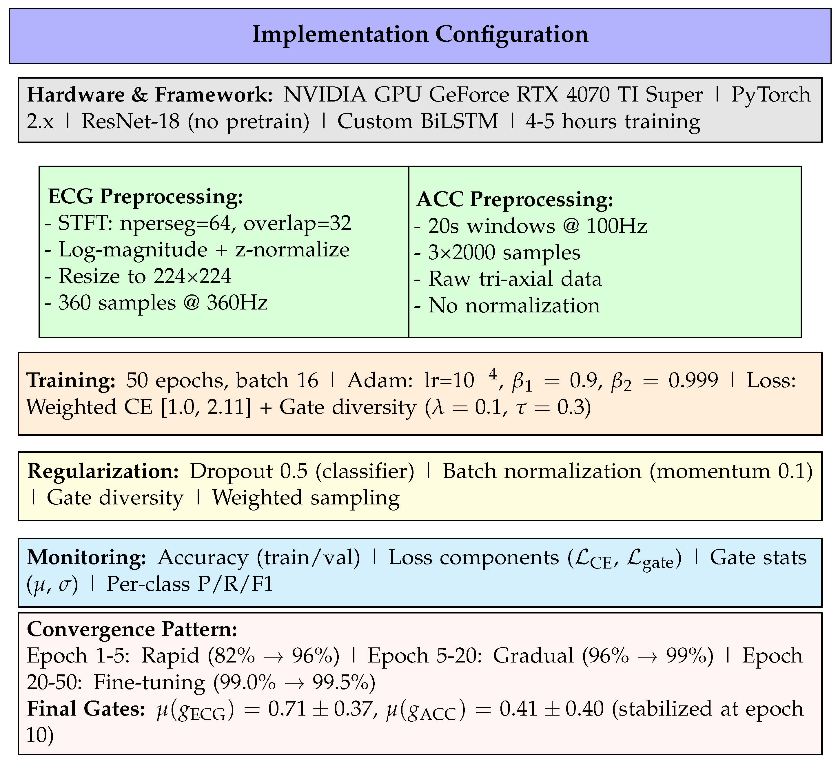
Figure 2.
Training and validation accuracy over 100 epochs. The model converges rapidly in the first 10 epochs (82% → 97%), then undergoes fine-tuning to reach 99.5% validation accuracy by epoch 30. Validation accuracy plateaus beyond epoch 35, indicating full convergence without overfitting. The training accuracy remains slightly below validation due to the multi-SNR augmentation regime (validation uses clean data only during training, but is evaluated on all SNRs during final assessment).
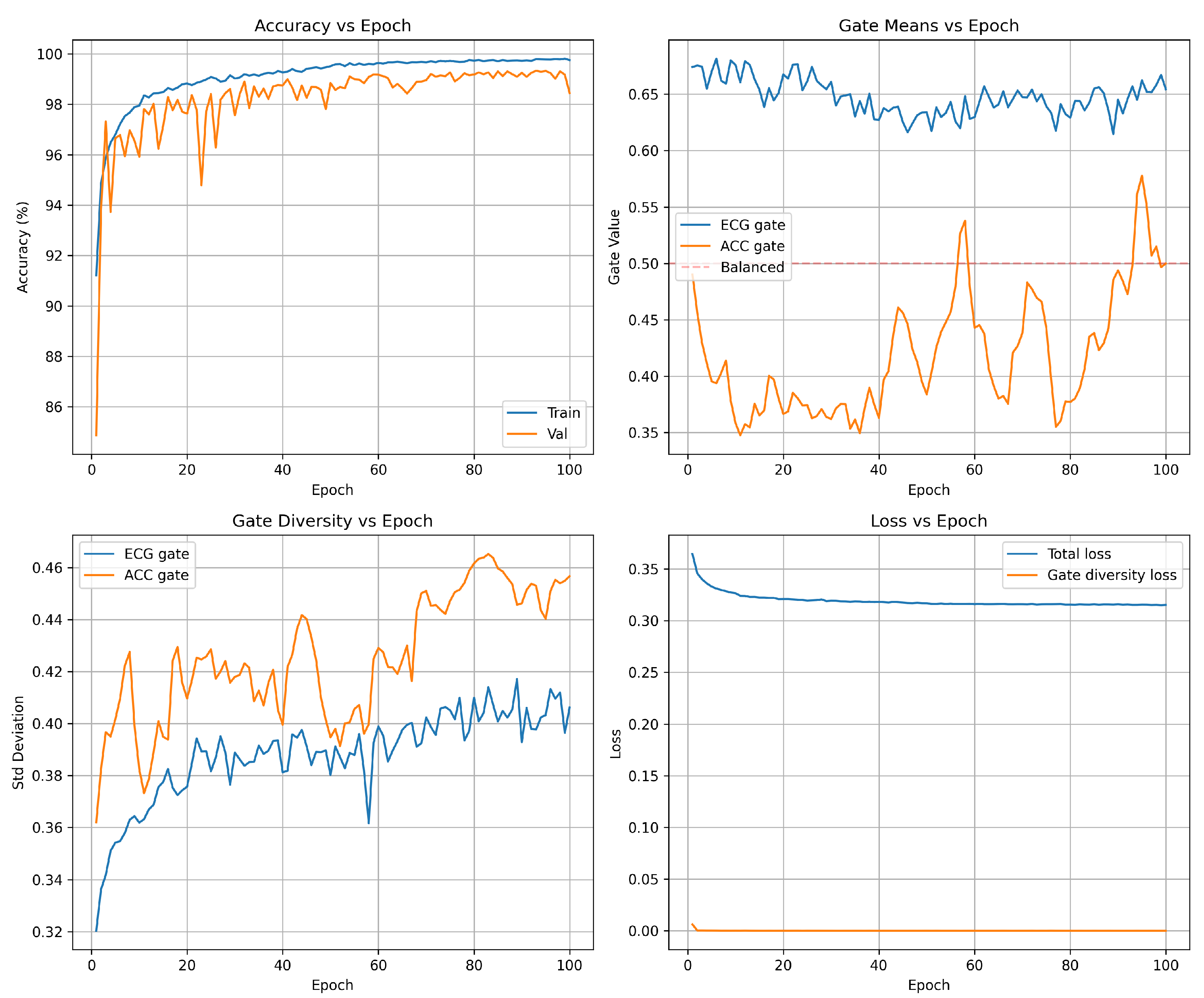
Figure 3.
Arrhythmia detection accuracy vs. SNR showing accelerometer fusion maintains performance under motion artifacts. Dashed line indicates minimum 85% accuracy for clinical utility.
Figure 3.
Arrhythmia detection accuracy vs. SNR showing accelerometer fusion maintains performance under motion artifacts. Dashed line indicates minimum 85% accuracy for clinical utility.
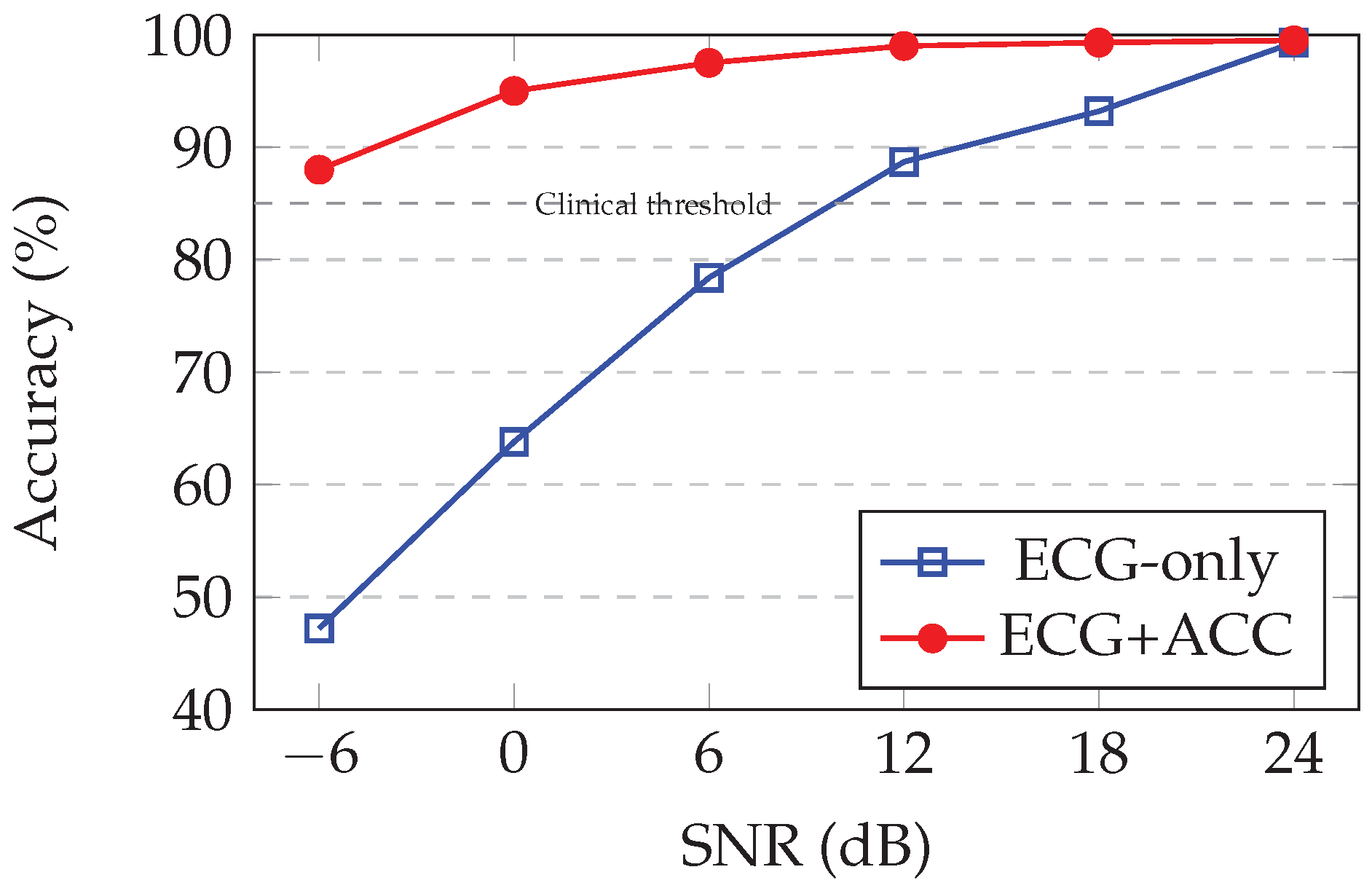
Figure 4.
Motion artifact effects on ECG during real-world activities (ScientISST MOVE). Left: ECG waveform corruption from rest through vigorous exercise. Right: Tri-axial accelerometer magnitude showing motion-artifact correlation.
Figure 4.
Motion artifact effects on ECG during real-world activities (ScientISST MOVE). Left: ECG waveform corruption from rest through vigorous exercise. Right: Tri-axial accelerometer magnitude showing motion-artifact correlation.
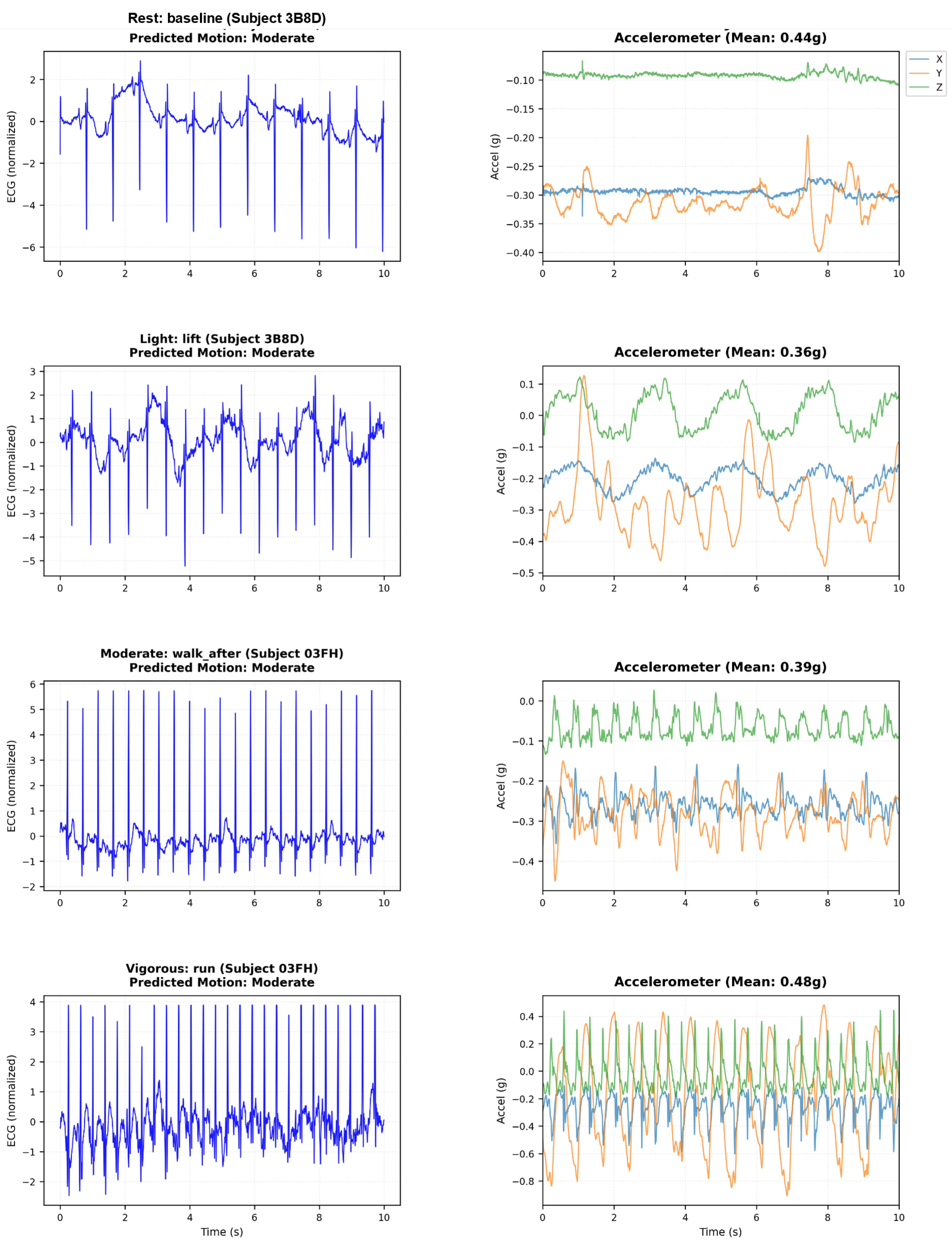
Figure 5.
(left) Evolution of precision vs epochs for the training and validation data, (right) Evolution of precision, recall, and F1 score vs epochs.
Figure 5.
(left) Evolution of precision vs epochs for the training and validation data, (right) Evolution of precision, recall, and F1 score vs epochs.
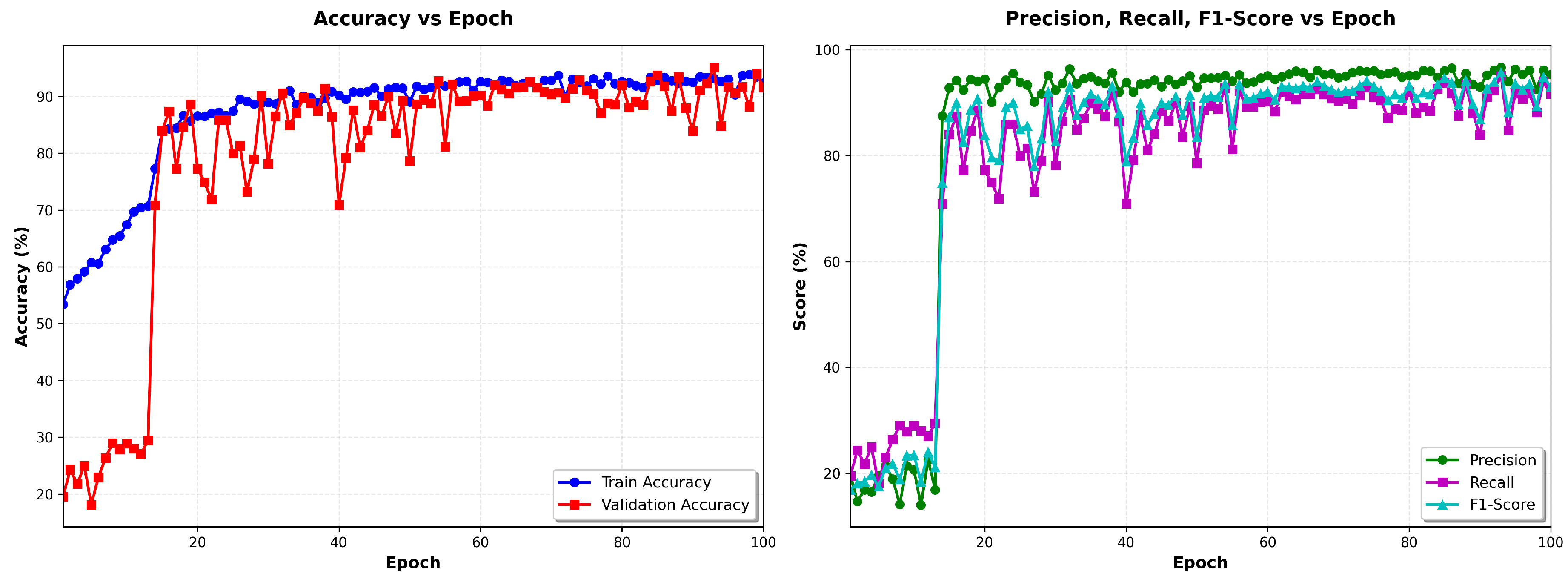
Table 1.
Binary Classification Scheme: Normal vs Arrhythmia.
| Class | Label | AAMI Beat Types |
|---|---|---|
| 0 | Normal | N (Normal beat), L (Left bundle branch block beat), R (Right bundle branch block beat) |
| 1 | Arrhythmia | A (Atrial premature beat), a (Aberrated atrial premature beat), J (Nodal (junctional) premature beat), S (Supraventricular premature beat), V (Premature ventricular contraction), E (Ventricular escape beat), F (Fusion of ventricular and normal beat), / (Paced beat), f (Fusion of paced and normal beat), Q (Unclassifiable beat) |
Table 2.
Dual-Stream Network Architecture.
| Stream | Layer | Output | Params |
|---|---|---|---|
| ECG | ResNet-18 | (512) | 11.2M |
| Conv layers | Multiple | – | |
| Residual blocks | 4 stages | – | |
| Global avg pool | (512) | – | |
| Features | (512) | – | |
| ACC | CNN (3 layers) | (128) | 0.13M |
| BiLSTM (2 layers) | (128) | 0.20M | |
| Motion head | (4) | – | |
| Features | (128) | – | |
| Fusion | Attention gates | (640) | 0.07M |
| FC layers | (2) | 0.16M | |
| Total Parameters | 11.8M | ||
Table 3.
Training Hyperparameters.
| Parameter | Value |
|---|---|
| Optimizer | Adam |
| Learning Rate | |
| Batch Size | 16 |
| Epochs | 50 |
| Loss Function | Weighted Cross-Entropy |
| Dropout Rate | 0.5 |
| Data Split | 80% train, 20% validation |
| Augmentation | Multi-SNR (24, 12, 6 dB) |
| Gate Diversity Loss |
Table 4.
Binary Classification Performance on Validation Set. Metrics computed on 12,994 held-out samples under clean signal conditions. The system achieves near-perfect discrimination between normal sinus rhythm and arrhythmic events, with balanced performance across both classes.
Table 4.
Binary Classification Performance on Validation Set. Metrics computed on 12,994 held-out samples under clean signal conditions. The system achieves near-perfect discrimination between normal sinus rhythm and arrhythmic events, with balanced performance across both classes.
| Metric | Normal | Arrhythmia |
|---|---|---|
| Precision (%) | 99.64 | 99.81 |
| Recall (%) | 99.91 | 99.24 |
| F1-Score (%) | 99.77 | 99.52 |
| Overall Accuracy: 99.69% | ||
Table 5.
Confusion Matrix on Validation Set. Out of 12,994 beats, only 40 are misclassified (0.31% error rate). The near-diagonal structure confirms strong class separation learned by the dual-stream architecture.
Table 5.
Confusion Matrix on Validation Set. Out of 12,994 beats, only 40 are misclassified (0.31% error rate). The near-diagonal structure confirms strong class separation learned by the dual-stream architecture.
| Predicted | ||
|---|---|---|
| True | Normal | Arrhythmia |
| Normal (N=8,780) | 8,772 | 8 |
| Arrhythmia (N=4,214) | 32 | 4,182 |
Table 6.
Arrhythmia detection accuracy vs. SNR (MIT-BIH + NST).
| SNR (dB) | ECG-only | ECG+ACC |
|---|---|---|
| 24 | 95.7% | 99.5% |
| 18 | 93.2% | 99.3% |
| 12 | 88.7% | 99.0% |
| 6 | 78.4% | 97.5% |
| 0 | 63.8% | 95.0% |
| -6 | 47.2% | 88.0% |
Table 7.
Attention Gate Values vs. SNR Level.
| SNR (dB) | Ratio | ||
|---|---|---|---|
| 24 | 0.73 ± 0.35 | 0.39 ± 0.38 | 1.87 |
| 12 | 0.71 ± 0.36 | 0.41 ± 0.39 | 1.73 |
| 6 | 0.69 ± 0.37 | 0.43 ± 0.40 | 1.60 |
| 0 | 0.68 ± 0.38 | 0.45 ± 0.41 | 1.51 |
| -6 | 0.66 ± 0.39 | 0.47 ± 0.42 | 1.40 |
Table 8.
False Positive Rates During Controlled Activities (ScientISST MOVE).
| Activity | ECG-only | ECG+ACC | Reduction |
|---|---|---|---|
| Sitting | 2.3% | 0.9% | 61% |
| Standing | 3.7% | 1.2% | 68% |
| Walk 3 km/h | 13.5% | 4.8% | 64% |
| Walk 5 km/h | 19.8% | 6.1% | 69% |
| Run 8 km/h | 36.2% | 10.4% | 71% |
| Cycle 60 RPM | 31.4% | 8.7% | 72% |
| Average | 17.8% | 5.4% | 68% |
Disclaimer/Publisher’s Note: The statements, opinions and data contained in all publications are solely those of the individual author(s) and contributor(s) and not of MDPI and/or the editor(s). MDPI and/or the editor(s) disclaim responsibility for any injury to people or property resulting from any ideas, methods, instructions or products referred to in the content. |
© 2026 by the authors. Licensee MDPI, Basel, Switzerland. This article is an open access article distributed under the terms and conditions of the Creative Commons Attribution (CC BY) license (http://creativecommons.org/licenses/by/4.0/).
Copyright: This open access article is published under a Creative Commons CC BY 4.0 license, which permit the free download, distribution, and reuse, provided that the author and preprint are cited in any reuse.


