Predicting Aircraft Monitoring Parameters Using Regression Polynomials with Process Similarity Criteria Fit

1. Introduction

The aircraft parts' reliability prediction is critical for aviation safety [1]. The set of machine learning methods provides a solid asset for predicting technological process abnormalities. The opportunity to diagnose the aircraft engine state in real-time mode with a neural network is covered in research papers [2,3]. The publications that compare the existing machine-learning approaches for aircraft health prediction are listed below. The paper [4] introduces a comparison of using three neural network methods for airplane cooling system health prediction:

• Fully Connected Autoencoder (FCAE): The FCAE used in this paper is a multi-layered neural network with an input layer and multiple hidden layers.
• .Convolutional Autoencoder (CAE). Using this model by following good results for anomaly detection using time series data in this research [5], the proposed CAE is a variant of the FCAE where fully connected and convolutional layers are mixed in the encoder and decoder.
• LSTM Autoencoder (LSTMAE), where layers consist of Long Short-Term Memory (LSTM) neural networks, allowing for input sequences to be of variable length. The theoretical aspects of the LSTM neural network are covered in [6].

Table 1. Neural network models precision in predicting the health of the airplane cooling system.

	LSTMAE	CAE	FCAE
Precision	85.8%	93.4%	97.1%

Table 1. Neural network models precision in predicting the health of the airplane cooling system.

	LSTMAE	CAE	FCAE
Precision	85.8%	93.4%	97.1%

Although FCAE and CAE precision is the highest, both models tend to reconstruct some of the anomalies with a high rate of false negatives and low recall. Per the author's conclusion, the added complexity of a CAE compared to an FCAE does not improve the performance; LSTMAE models are more precise and superior overall.

The research paper [7] compares such machine learning methodologies as LSTM, Random Forest, Gaussian Regression (RFGR) [8], Linear Regression (LR), K-Nearest Neighbours Regression (K-NNR), and Support Vector Regression (SVR) to predict engine health.

The accuracy and precision of the methods are shown in the table below.

Table 2. Aircraft engine health prediction comparable results using machine learning methods.

	LR (%)	K-NNR (%)	SVR (%)	GR (%)	RF (%)	LSTM (%)
Accuracy	74.5	76.4	78.1	92.4	92.8	98.9
Precision				79.98	90.13	93.88

Table 2. Aircraft engine health prediction comparable results using machine learning methods.

	LR (%)	K-NNR (%)	SVR (%)	GR (%)	RF (%)	LSTM (%)
Accuracy	74.5	76.4	78.1	92.4	92.8	98.9
Precision				79.98	90.13	93.88

Both models conclude that the LSTM has the best prediction result. For this reason, we will compare the new rapid prediction approach with the LSTM model.

Using LSTM, Random Forest, and Gaussian Regression methods is highly efficient for predicting the health of the system, which does not require rapid diagnostics.

The limitations of Machine Learning approaches covered above for rapid forecasting related to the training time. Modern aircraft are often equipped with thousands of sensors, and full flight sensor data with thousands of parameters is recorded for each flight [1]. The number of sensors that read critical aircraft parameters that can be rapidly changed and lead to catastrophic events is significant for using high-time complexity algorithms for onboard computing. The research paper [9] covers real-time engine health diagnostics by sending monitoring data to the nearest EMC labs and processing data using a high-performance computing model. Boeing 777 engine sensors generate around 200 gigabytes of data every minute. Transmitting such data in real-time requires considerable bandwidth, which may be limited or costly, especially via satellite communication [3].

The advantage of the RPPSCF is its low computational complexity and high accuracy, according to research results for thermal process prediction [10]. This makes the method a promising candidate for real-time prediction of aircraft parameters. The method is also flexible for prediction accuracy optimization by redefining similarity criteria.

2. Predicting Aircraft Parameters Using Regression Polynomials with the Process Similarity Criteria Fit

The RPPSCF method [10,11] for stochastic data defined with dynamic hypernumber $H_k$ satisfactory conditions, is listed below:

• The polynomial should satisfy statistical criteria. The time series data point filtered from the stochastic noise should belong to the polynomial.
• The last point of the training time series data is defined with the condition: $H_k\left(t_n\right)= \overline{P}\left(t_n\right)$

The equal variance statistical criterion is defined by expression 1.

$$L=min\sum _{i=0}^n{\left( {\displaystyle \frac{\sum _{j=i-\frac{m}{2}}^{j=i+\frac{m}{2}}{\left(P_j-\left(a_{0+}{a}_1{t}_j+\dots +a_l{t}_j^{l }\right)\right)}^2}{m-1}}-\overline{v}\right)}^2$$

(1)

where $P_j$ is monitoring sequential parameter’s value and $\overline{v}$ is a variance defined with the expression:

$$\overline{v}={\displaystyle \frac{1}{n}}\sum _{i=1}^n{\left(P_i-\left(a_{0 + }{a}_1{t}_j+ a_2{t}_j^2+ \dots + a_l{t}_j^{l }\right)\right)}^2$$

(2)

Let the sum of the time-dependent member of the regression polynomial equal:

$${S_n=a}_{1 }\left(t_i- t_n\right)+ a_{2 }\left(t_i^2- t_n^2\right)+ {\dots + a}_n\left(t_i^n- t_l^n\right)$$

(3)

Plugging (3) into (2) yields expression (3) for a variance results:

$$\overline{v}={\displaystyle \frac{1}{n}}\sum _{i=1}^n{\left(P_i- \left(S_n+ H_k\left(t_n\right)\right)\right)}^2$$

(4)

where $H_k\left(t_n\right)$ is defined with linear regression of the $P_i$ . The $H_k\left(t_n\right)$precision can be calculated using Least Squares Error estimation [12].

The conditions (5) should be satisfied for an operator (1)

$$\left\{\begin{array}{c}{\displaystyle \frac{\partial L}{\partial a_1}}=0\\ {\displaystyle \frac{\partial L}{\partial a_2}}=0\\ \begin{array}{c}\dots \\ \begin{array}{c}{\displaystyle \frac{\partial L}{\partial a_r}}=0\\ \begin{array}{c}\dots \\ {\displaystyle \frac{\partial L}{\partial a_l}}=0\end{array}\end{array}\end{array}\end{array}\right.$$

(5)

The operator L derivative for arbitrary polynomial coefficient is calculated with the expression below:

$$\begin{gathered} {\displaystyle \frac{\partial L}{\partial a_r}}=2\sum _{i=0}^n\left({\displaystyle \frac{\sum _{j=i-\frac{m}{2}}^{j=i+\frac{m}{2}}{\left(P_j-\left(S_n+ H_k\left(t_n\right)\right)\right)}^2}{m-1}} \\ \hspace{1em}\hspace{1em}\hspace{1em}\hspace{1em}\hspace{1em}\hspace{1em}\hspace{1em}\hspace{1em}\hspace{1em}\hspace{1em}\hspace{1em}\hspace{1em}\hspace{1em}\hspace{1em}\hspace{1em}\hspace{1em}\hspace{1em}-\overline{v}\right)\left(\sum _{j=i-{\displaystyle \frac{m}{2}}}^{j=i+{\displaystyle \frac{m}{2}}}{\displaystyle \frac{-2\left(P_j-\left(S_n+ H_k\left(t_n\right)\right)\right)\left(t_j^{n-r}-t_n^{n-r}\right)}{m-1}}-{\displaystyle \frac{\partial \overline{v}}{\partial a_r}}\right)=0 \end{gathered}$$

(6)

To simplify the expression, the term ${∆P}_j$ is defined as:

$${∆P}_j= P_j-\left(S_n+ H_k\left(t_n\right)\right)$$

(7)

The expression below is obtained by plugging (7) into (6):

$${\displaystyle \frac{\partial L}{\partial a_r}}=2\left(\sum _{j=i-{\displaystyle \frac{m}{2}}}^{j=i+{\displaystyle \frac{m}{2}}}{\displaystyle \frac{{∆P}_j}{m-1}} -\overline{v}\right)\left(\sum _{j=i-{\displaystyle \frac{m}{2}}}^{j=i+{\displaystyle \frac{m}{2}}}{\displaystyle \frac{-2{∆P}_j\left(t_j^{n-r}-t_n^{n-r}\right)}{m-1}} -{\displaystyle \frac{\partial \overline{v}}{\partial a_r}}\right)$$

(8)

The ${\displaystyle \frac{\partial \overline{v}}{\partial a_r}}$ is computed by plugging (3) into (4)

$${\displaystyle \frac{\partial \overline{v}}{\partial a_r}}={\displaystyle \frac{-2}{n}}\sum _{i=1}^n{∆P}_j\left(t_i^{n-r}-t_n^{n-r}\right)$$

(9)

The iteration of finding a polynomial using operator equations solutions with the theory of hypernumber [13,14] is defined below.

$$H_{k+1}^{con}=H_k^{con}+\delta H_k^{con}$$

(10)

where $\delta H_k^{con}$ is the deviation to find the new value of the polynomial. defined with matrices equation:

$$\delta H_k^{con}=-\epsilon \times {DL}_k \times {LM}_k^{-1}$$

(11)

where DL and LM matrices are computed using equations (12, 13)

$${DL}_k=\left|\begin{array}{c}{\displaystyle \frac{\partial L}{\partial a_1}}\left(H_k\right)\\ {\displaystyle \frac{\partial L}{\partial a_2}}\left(H_k\right)\\ \begin{array}{c}\dots \\ {\displaystyle \frac{\partial L}{\partial a_l}}\left(H_k\right)\end{array}\end{array}\right|$$

(12)

$${LM}_k=\left|\begin{array}{c}\begin{array}{cc}{\displaystyle \frac{{\partial }^{2}L}{{\left(\partial a_1\right)}^2}}\left(H_k\right)& \begin{array}{cc}\dots & {\displaystyle \frac{{\partial }^{2}L}{\left(\partial a_1\right)\left(\partial a_l\right)}}\left(H_k\right)\end{array}\\ {\displaystyle \frac{{\partial }^{2}L}{\left(\partial a_1\right)\left(\partial a_2\right)}}\left(H_k\right)& \begin{array}{cc}\dots & {\displaystyle \frac{{\partial }^{2}L}{\left(\partial a_2\right)\left(\partial a_3\right)}}\left(H_k\right)\end{array}\\ \dots & \begin{array}{cc} & \dots \end{array}\end{array}\\ \begin{array}{cc}{\displaystyle \frac{{\partial }^{2}L}{\left(\partial a_1\right)\left(\partial a_l\right)}}\left(H_k\right)& \begin{array}{cc}\dots & {\displaystyle \frac{{\partial }^{2}L}{{\left(\partial a_l\right)}^2}}\left(H_k\right)\end{array}\end{array}\end{array}\right|$$

(13)

The ${\displaystyle \frac{{\partial }^{2}L}{\partial a_r\partial a_c}}$ expression is defined by taking derivative from (8)

$$\begin{gathered} {\displaystyle \frac{{\partial }^{2}L}{\partial a_r\partial a_c}}=\sum _{i=0}^n\left({\displaystyle \frac{\sum _{j=i-\frac{m}{2}}^{j=i+\frac{m}{2}}{\left({∆P}_j\right)}^2}{m-1}}-\overline{v}\right)\times \\ \hspace{1em}\hspace{1em}\hspace{1em}\hspace{1em}\hspace{1em}\left({\displaystyle \frac{2}{m-1}}\sum _{j=i-{\displaystyle \frac{m}{2}}}^{j=i+{\displaystyle \frac{m}{2}}}\left(t_j^{l-r}-t_n^{l-r}\right)\left(t_j^{l-c}-t_n^{l-c}\right) – {\displaystyle \frac{{\partial }^2\overline{v}}{\partial a_r\partial a_c}}\right)+ \\ \hspace{1em}\hspace{1em}\hspace{1em}\hspace{1em}\hspace{1em}\hspace{1em}\hspace{1em} \left(\sum _{j=i-{\displaystyle \frac{m}{2}}}^{j=i+{\displaystyle \frac{m}{2}}}{\displaystyle \frac{2{∆P}_j}{m-1}}+{\displaystyle \frac{\partial \overline{v}}{\partial a_c}}\right)\times \left(\sum _{j=i-{\displaystyle \frac{m}{2}}}^{j=i+{\displaystyle \frac{m}{2}}}{\displaystyle \frac{2{∆P}_j\left(t_j^{l-r}-t_n^{l-r}\right)}{m-1}}+{\displaystyle \frac{\partial \overline{v}}{\partial a_r}}\right) \end{gathered}$$

(14)

The ${\displaystyle \frac{{\partial }^2\overline{v}}{\partial a_r\partial a_c}}$ derivative is provided below:

$${\displaystyle \frac{{\partial }^2\overline{v}}{\partial a_r\partial a_c}}= {\displaystyle \frac{2}{n}}\sum _{i=1}^n\left(t_i^{l-r}- t_n^{l-r}\right)\left(t_i^{l-c}- t_n^{l-c}\right)$$

(15)

It has been proven in [13] that there exists $\epsilon <1$ such that guarantees convergence of the solution to the operator equation using constructive hypernumber.

3. Predicting Aircraft Engine Parameters with Similarity Criteria Fit

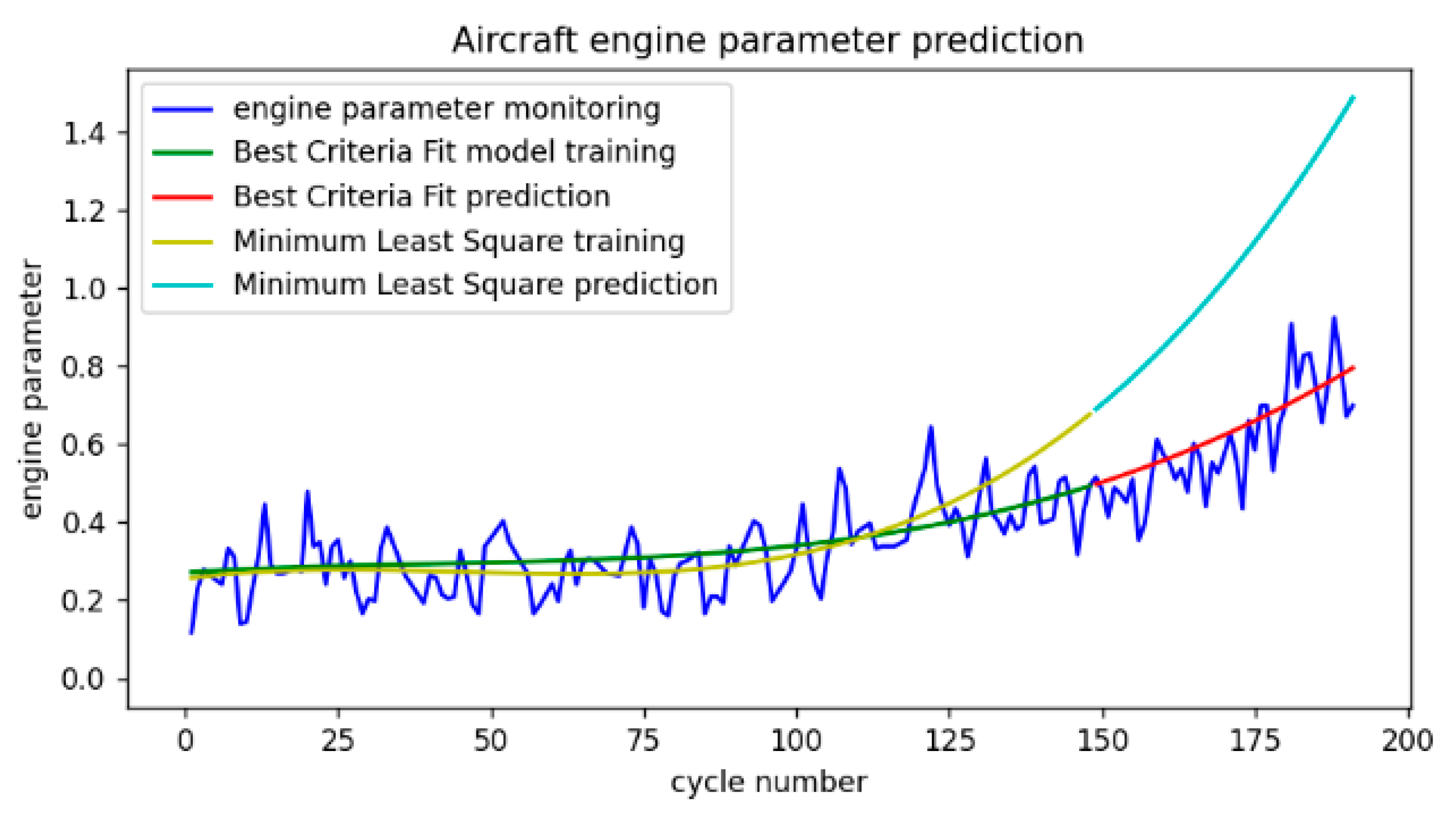
For engine parameters prediction with Similarity Criteria Fit, polynomial power 3 was selected. The formulas (3,4,6-15) are used to compute the polynomial. The results of the aircraft parameter prediction using RPPSCF and regular minimum least square methods are compared and shown in Figure 1. The simulation shows high prediction accuracy (86.9%) of the Similarity Criteria methods.

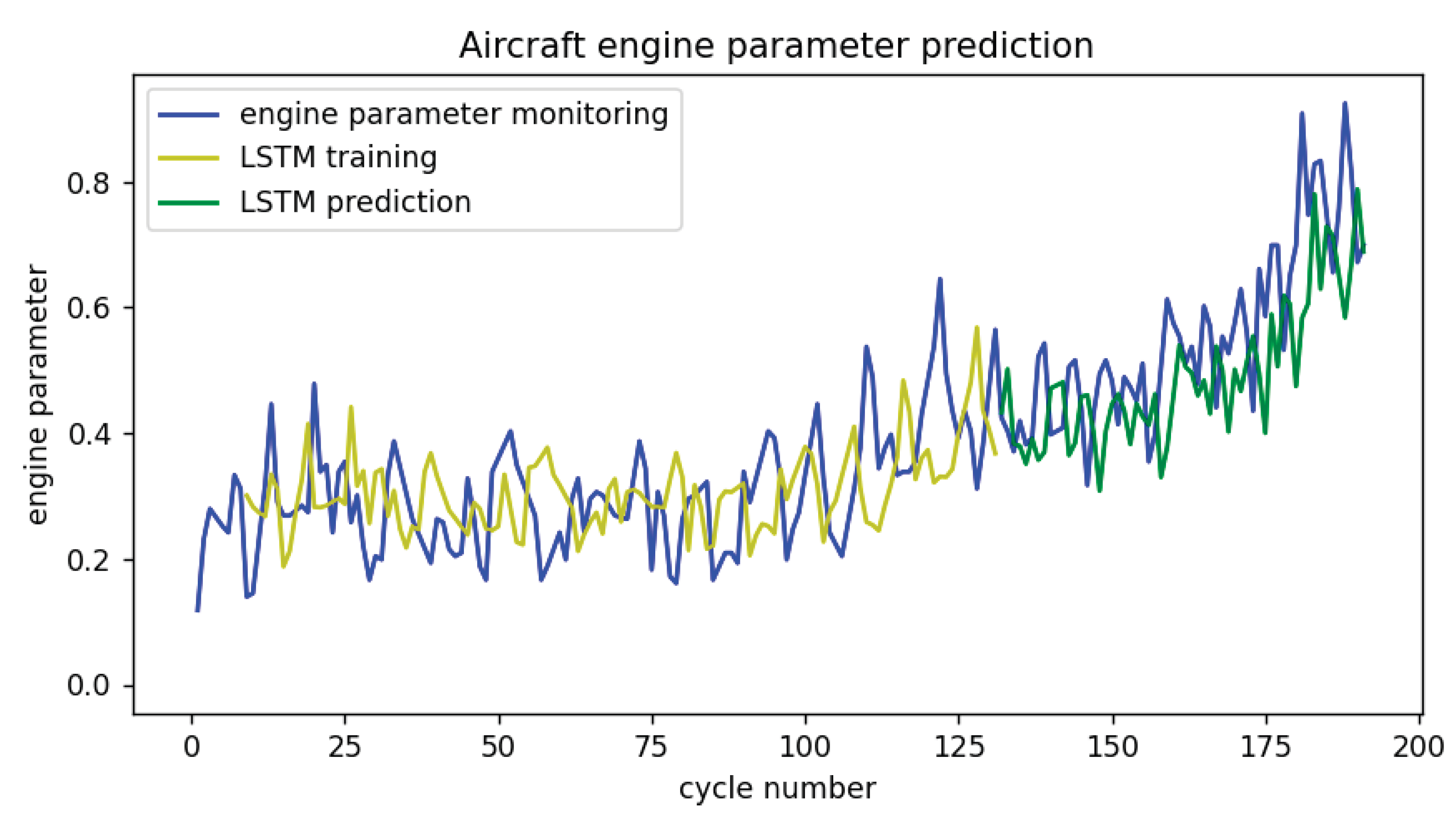
The aircraft engine parameter prediction for the same data set was done using the LSTM neural network model. The prediction results are shown in Fig. 2. Such a prediction was implemented to compare the most efficient aircraft engine prediction and rapid real-time diagnostics by Regression with Process Similarity Criteria Fit methods. The accuracy of the LSTM model, per such simulation, is 88.0%. Per both methods' close precisions, the RPPSCF method is approximately 30 times faster than the LSTM prediction.

Figure 2. Predicting aircraft engine parameters with LSTM model.

Figure 2. Predicting aircraft engine parameters with LSTM model.

4. Results and Discussion

Considering the RPPSCF method’s accuracy and performance, it can be used for a real-time prediction of the aircraft's life-critical parameters to detect abnormalities and prevent catastrophic events. At the same time, due to the high volume of monitoring data, the method can be an alternative for maintenance prediction. Besides hypernumber methods for solving non-linear equations, the Modified Newton (Kantorovich’s) method can be used if the convergence conditions are satisfied [15,16,17]. The conditions can be verified in real time. The advantage of Kantorovich’s method is rapid computation time. However, contrary to Kantorovich’s method, the hypernumber method works for arbitrary time series data sequences.

The process similarity criteria defined for engine parameter analysis in this paper assumes equal variance. The simulation results support this selection. However, for some processes, the variance could be time-dependent on parameters. Defining the function of the variance time dependency is a subject of future research.

5. Conclusions

The high accuracy and low computational complexity of the intrudeced method’s prove it’s applicability for real time aircraft parts failure prediction The method can be also extended for processes where the variance is time depended by defining it’s approximation and plugging such function into the expression (1) for an operator $L$. The methodics for variance approximation will be defined in future research. One of the considered approach reveals to applying RPPSCF method using variance of variance for an approximation [18].

On the contrary to the neural network, the method provides analytical expression for predicting monitoring parameters, which allows automatically control processes.

Each Machine Learning method has some cognition limitations. The provided PRPSCF method in provided definition as well as not Physics-Informed Neural Networs (PiNNs) [19] is not able to predict periodic processes. However, the presented concept can be used for non-stationary periodic prediction combining Wavelet Transform and defined process criteria.

References

- Wang, C.; Puigh, D.; Lei, A.; Guo, W.; Yuan, J.; Mazarek, M. Lessons Learned from Aircraft Component Failure Prediction Using Full Flight Sensor Data. PHM Sociaty Asia-Pacific Conference 2023, 4, 3684. [Google Scholar] [CrossRef]
- Darrah, T.; Lovberg, A.; Frank, J.; Biswas, G.; Quinones-Gruiero, M. Developing Deep Learning Model for System Remaining Useful Life Predictions: Application to Aircraft Engines. Annual Conference of the PHM Society 2022, 14. [Google Scholar] [CrossRef]
- Kabashkin, I.; Perekrestov, V. Ecosystem of Aviation +Maintenance: Transition from Aircraft Health Monitoring to Health Management Based on IoT and AI Synergy. Appl. Sci. 2024, 14, 4394. [Google Scholar] [CrossRef]
- Basora, L.; Bry, P.; Olive, X.; Freeman, F. Aircraft Fleet Health Monitoring with Anomaly Detection Techniques. Aerospace 2024, 8, 103–136. [Google Scholar] [CrossRef]
- Husebø, A.B.; Kandukuri, S.T.; Klausen, A.; Robbersmyr, K.G. Rapid Diagnosis of Induction Motor Electrical Faults using Convolutional Autoencoder Feature Extraction. PHM Society European Conference 2020, 5, 10–10. [Google Scholar] [CrossRef]
- Elsworth, S.; Guttel, S. Time Series Forecasting Using LSTM Networks: A Symbolic Approach. Available online: https://arxiv.org/pdf/2003.05672.
- Yildirim, S.; Rana, Z. Enhancing Aircraft Safety through Advanced Engine Health Monitoring with Long Short-Term Memory. Sensors 2024, 24, 518–518. [Google Scholar] [CrossRef] [PubMed]
- Chopra, P. Gaussian Processes for Modeling Time-series Supplier Distribution Costs. M.S. Thesis, Uppsala University, SE-751 05 Uppsala, Sweden, 2021. [Google Scholar]
- Essa, Y.; Attiya, G.; El-Sayed, A. Real Time Analysis for Aircraft Using EMC Labs. [Online]; Proven Professional Knowledge Sharing, USA, 2015. 2015. Available online: https://www.researchgate.net/publication/302580400_REAL_TIME_ANALYSIS_FOR_AIRCRAFT_USING_EMC_LABS (accessed on 17 May 2024).
- Dantsker, A.; Brito, J.; Pryor, W. Defining Regression Polynomials with Process Similarity Criteria. RRDMS 2023, 10, 13–20. [Google Scholar] [CrossRef]
- Burgin, M.; Dantsker, A.; Pryor, W. Detecting Electronic Circuit board Thermal Abnormalities with Dynamic Hypernumbers. RRDMS 2023, 10. [Google Scholar] [CrossRef]
- Richter, P. Estimating Errors in Least-Squares Fitting. 1995. Available online: https://ipnpr.jpl.nasa.gov/progress_report/42-122/122E.pdf (accessed on 26 February 2025).
- Burgin, M.; Dantsker, A. A method of solvi;g operator equations of mechanics with the theory of Hypernumbers. Notices of the National Academy of Sciences of Ukraine 1995, 8, 27–30. [Google Scholar]
- Burgin M. Operations with Extrafunctions and Integration in Bundles with a Hyperspace Base. Functional Analysis and Probability. In Chapter 1; Nova Science Publishers: New York, 2015.
- Kantorovich, L.V.; Akilov, G.P. Functional Analysis, 2nd ed.; Pergamon Press: Oxford, 1982. [Google Scholar]
- Regmi, S.; Arguros, I. K.; George, S.; Arguros, C. I. Extended Newton-Kantorovich Theorem for Solving Nonlinear Equations. Fondations 2022, 2, 504–511. [Google Scholar] [CrossRef]
- Regmi, S.; Argyros, I.; George, S.; & Argyros, M. Extended Regmi, S.; Argyros, I.; George, S.; & Argyros, M. Extended Kantorovich Theory for Solving Nonlinear equations with applications. Comput. Appl. Math. 2023, 42. [CrossRef]
- Cho, E.; Cho, M. Variance of Sample Variance. Section on Survey Research Method - JSM 2008, 1291–1293. Available online: http://www.asasrms.org/Proceedings/y2008/Files/3000992.pdf.
- Raissi, M.; Perdikaris, P.; Karniadakis, G.E. Physics-Informed Neural Networs: A Deep Learning Framework for Solving Forward and Inverse Problems Involving Nonliear Partial Differential Equations. J. Comput. Phys. 2019, 378, 686–707. [Google Scholar] [CrossRef]
Figure 1.
Comparative analysis of the aircraft engine prediction with the Minimum Least. Squares and Best Criteria Fit models.
Disclaimer/Publisher’s Note: The statements, opinions and data contained in all publications are solely those of the individual author(s) and contributor(s) and not of MDPI and/or the editor(s). MDPI and/or the editor(s) disclaim responsibility for any injury to people or property resulting from any ideas, methods, instructions or products referred to in the content. |
© 2026 by the authors. Licensee MDPI, Basel, Switzerland. This article is an open access article distributed under the terms and conditions of the Creative Commons Attribution (CC BY) license (http://creativecommons.org/licenses/by/4.0/).
Copyright: This open access article is published under a Creative Commons CC BY 4.0 license, which permit the free download, distribution, and reuse, provided that the author and preprint are cited in any reuse.