
Submitted:
08 January 2026
Posted:
09 January 2026
You are already at the latest version
Abstract
Fermi arcs appear as the surface states at the boundary of a three-dimensional topological semimetal with the vacuum, reflecting the Chern number (C) of a nodal point in the momentum space, which represents singularities (in the form of monopoles) of the Berry curvature. They are finite arcs, attaching/reattaching with the bulk-energy states at the tangents of the projections of the Fermi surfaces of the bands meeting at the nodes. The number of Fermi arcs grazing onto the tangents of the outermost projection equals C, revealing the intrinsic topology of the underlying bandstructure, which can be visualised in experiments like ARPES. Here we outline a generic procedure to compute these states for generic nodal points, (1) whose degeneracy might be twofold or multifold; and (2) the associated bands might exhibit isotropic or anisotropic, linear- or nonlinear-in-momentum dispersion. This also allows us to determine whether we should get any Fermi arcs at all for C = 0, when the nodes host ideal dipoles.
Keywords:
berry curvature
; fermi arcs
; surface states
; topology
Nodal points (NPs) in three-dimensional (3d) semimetals represent defective points in the Brillouin zone (BZ), where cross at a nodal-point degeneracy [see Figure 1(a)]. In the vicinity of a nodal point, the bands form a spin- representation of the SU(2) group. They provide an intriguing crucible to observe mathematical notions of topology playing out in real-life systems [1,2,3,4,5,6,7,8,9,10] because they are the singular points of the Berry-curvature (BC) where it blows up, hosting a BC-monopole synonymous with the net Chern number () at the NP. An isotropic Weyl node, appearing in semimetals (WSMs) [1,3,5], carrying , is the poster child of such systems, depicting the simplest scenario. The ubiquitousness of the NPs is reflected by WSMs’ multifold cousins like the triple-point semimetals (with ) and Rarita-Schwinger-Weyl (RSW) nodes (with ) [7,9,11,12,13,14,15,16,17,18]. The singularity of the BC at an NP [19,20,21] goes beyond the monopole-character, as the possibility of ideal BC-dipoles and higher-order poles have been predicted [22,23,24,25], when considering a multipole expansion of the Berry connection [cf. Figure 1(b)].
Often our study of the intrinsic topology of the 3d BZ, when treated as a 3d manifold, involves identifying unambigous quantitative signatures of the topological invariants like . Arguably Fermi arcs provide the most undisputed observables [26,27,28,29,30,31,32,33], as contemporary experiments like angle-resolved photoemission spectroscopy (ARPES) can clearly visualise them. Physically, they emerge as the loci of the surface edge-states when we take a surface (say, whose outward normal is along the unit vector, ) of a slab of a topological semimetal. In fact, these surface states arise due to the presence of chiral edge modes in 2d slices of the 3d BZ, after we impose open boundary conditions on those slices [1,2,4]. Although we can no longer describe the system in the momentum space for the direction along , the momentum-components perpendicular-to- (say, ), i.e., parallel to the surface itself, remain good quantum numbers (as long as we consider very large spatial dimensions along those directions). Thus, a single (boundary) surface in real space gives us an SBZ, spanned by the components of , and hosting the Fermi arcs. Although the analytical derivation of surface states, which take the form of Fermi arcs in NPs, is well-understood for the case of Weyl semimetals [34,35,36,37], for most other cases, the derivations are system-specific and not generic-enough [34,38,39,40,41,42] to be applicable for arbitrary cases of dispersion (for example, anisotropic and/or nonlinear-in-momentum behaviour) and band-crossings. In this Letter, our aim is to outline a generic procedure to obtain the analytical forms of the Fermi arcs and demonstrate its effectiveness by applying it to a variety of NPs.
Let us take a single surface at such that the region represent a semi-infinite semimetal, with the bulk Hamiltonian , where and . The translation symmetry is broken along the x-axis, and we use the Hamiltonian, . Demanding that be Hermitian in the region , we have the physical condition that
while considering two bonafide boundary-states, and . The current-density operator is defined as . Consequently, Eq. (1) also translates into a physically-sensible boundary condition which prohibits the current transmission through the boundary via , alternatively known as the hard-wall bc. The boundary modes must behave as decaying wavefunctions of the form of , so that the surface states are bound to the boundary at . Here, is independent of x and any x-dependence of is assumed to be contained in the factor.
The effective Hamiltonian in the vicinity of a single Weyl node [cf. Figure 1(a)] is captured by
for which Eq. (1) translates into . Witten [34] prescribed an energy-independent boundary condition,
as a local linear restriction on the components of the spinor wave function. This is a good boundary condition because anticommutes with M, leading to .
For generic nodes with multifold nodes and/or nonlinear powers of the components of , Witten’s trick will not work, which we will explicitly see why considering some specific examples. Hence, we need an unambigous generic method applicable to derive the equations describing the curves representing the relevant Fermi arcs, which we describe here. Suppose we have an N-fold degeneracy at a node, described by the Hamiltonian, in the bulk BZ. Let us look for surface states where the surface-normal is along the direction denoted by the unit vector, , and located at , where . We set our convention that the region represents the region occupied by the semimetallic material, while represents the adjoining non-topological region (e.g., vacuum). Dividing up the momentum components along and perpendicular to as and , the boundary Hamiltonian is obtained as . The imposition of the Hermiticity condition on leads to
analogous to Eq. (1). Let us parametrise a solution as
As argued earlier, will turn out to be equivalent to the condition of
represents the current-density operator perpendicular to the surface. Next, we need to solve for the eigenvalue equation,
which leads to N complex-valued equations involving the unknown variables E, , , , , , , …, , and . This implies that we have real equations [on including the real equation coming from Eq. (6)] at our disposal, which we can use to solve for the same number of unknown variables. In the next section, we will study a variety of systems to see that the above procedure works generically.
Let us consider the one-node model given by Eq. (2), where we want to consider a boundary at , indicating . Using , we get , , and . The bulk Hamiltonian in the vicinity of a node, tilted with respect to the -axis, is captured by . For this case, on using , we obtain the solutions as , , , and . Figure 2(a) illustrates the Fermi arcs for four distinct values of , with set to .
Let us now consider bands carrying pseudospin-1 quantum numbers crossing at threefold-degenerate nodes [7,9,43,44,45,46,47], representing the so-called triple-point semimetals (TSMs). These are three-band generalisations of the pseudospin-1/2 quasiparticles in Weyl semimetals, with the nodal points acting as Berry-curvature monopoles of magnitude 2. The effective low-energy continuum Hamiltonian, in the vicinity of a threefold nodal point, is given by , where represents the vector spin-1 operator with three components [45,46,47]. Here we note that, although this is a straightforward generalisation of the isotropic Weyl node, we cannot apply Witten’s method simply because of the fact that , , and do not anticommute (unlike the Pauli matrices). We use the parametrisation and consider a boundary at . Plugging it in Eqs. (6) and Eq. (7), the solutions indeed tell us that there are two Fermi arcs characterised by (1) , , , , , , and ; and (2) , , , , , , and . Figure 2(b) illustrates the Fermi arcs for and . Since , we observe two arcs entering into the FS-projection.
Next we focus on bands carrying pseudospin-3/2 quantum numbers crossing at fourfold-degenerate degenracy-points [cf. Figure 3(a)], widely known as the Rarita-Schwinger-Weyl (RSW) nodes. They appear at the -points of chiral crystals with appreciable SOC couplings [9,16,17,31,47,48], hosting a net BC-monopole of magnitude 4. The effective Hamiltonian, in the vicinity of an isotropic RSW node, takes the form of
, where represents the vector operator whose three components comprise the angular-momentum operators in the spin- representation of the SU(2) group. Just for the ease of calculations, we consider a boundary at (just because the matrix has fewer nonzero entries, leading to less cumbersome equations to be solved). Here again we note that, although this is a fourfold generalisation of the isotropic Weyl node, we cannot apply Witten’s method since , , and do not anticommute. We use the parametrisation because of the fourfold nature of the bands. Plugging it Eqs. (6) and Eq. (7) yield the explicit solutions which are long and cumbersome. In Figure 2(c), we pictorially show them for a specific case.
Double-Weyl nodes can be found in materials like [49] and [50,51]), which exhibits a hybrid of linear dispersion (chosen to be the -axis) and quadratic dispersion (in the -plane). In the vicinity of such a nodal point, the low-energy effective continuum Hamiltonian is given by [7,8,52,53,54,55,56] , where . Plugging in the parametrisation of in Eq. (6) leads to: , , , where and , where and . Figure 3(a) illustrates the Fermi arcs for and . Since , we observe two arcs emanating from the perimeter of the FS-projection.
Analogous to the double-Weyl nodes, there exist triple-Weyl nodes (in materials like transition-metal monochalcogenides [57]) for which . The triple-Weyl case comprises a hybrid of linear dispersion (chosen to be the -axis) and quadratic dispersion (in the -plane). In the vicinity of such a nodal point, the low-energy effective continuum Hamiltonian is given by [7,8,52,53,54,55,58] , where . Plugging in the parametrisation of leads to the required equations. Finding exact analytical solutions is cumbersome because of the cubit roots involved. Instead, we parametrise and , and we show below the solutions for : (1) , , , and ; (2) , , , and , where . Figure 3(b) illustrates the 3 Fermi arcs for and for the solution detailed above.
In a specific two-band model, the low-energy effective Hamiltonian in the vicinity of a single node harbouring a Berry-dipole [cf. Figure 3(b)] is captured by [22] . Since this is a two-band model, we again use . We obtain the solutions as , , , and . The points on the SBZ where goes to zero are antipodal points, whose tangents are . This shows one arc is leaving and another is entering into the bulk states which are located at the two hemispheres of the FS and which yield on integrating the BC-flux on their surfaces. This reflects the intrinctic dipole-character with . Figure 3(c) illustrates the scenario.
In Ref. [23], massless multifold Hopf semimetals have been introduced which host BC-dipoles at nodes where linearly-dispersing bands cross. We consider the simplest case with threefold-degenerate node, captured by the effective continuum Hamiltonian [23,24,25], , where
For this 3-band model, we use the parametrisation . The solutions turn out to be , , , , and . Figure 3(d) demonstrates the nature of the Fermi arcs for some distinct values of , which again leads to the picture that one arc is entering and the other leaving the bulk-states.
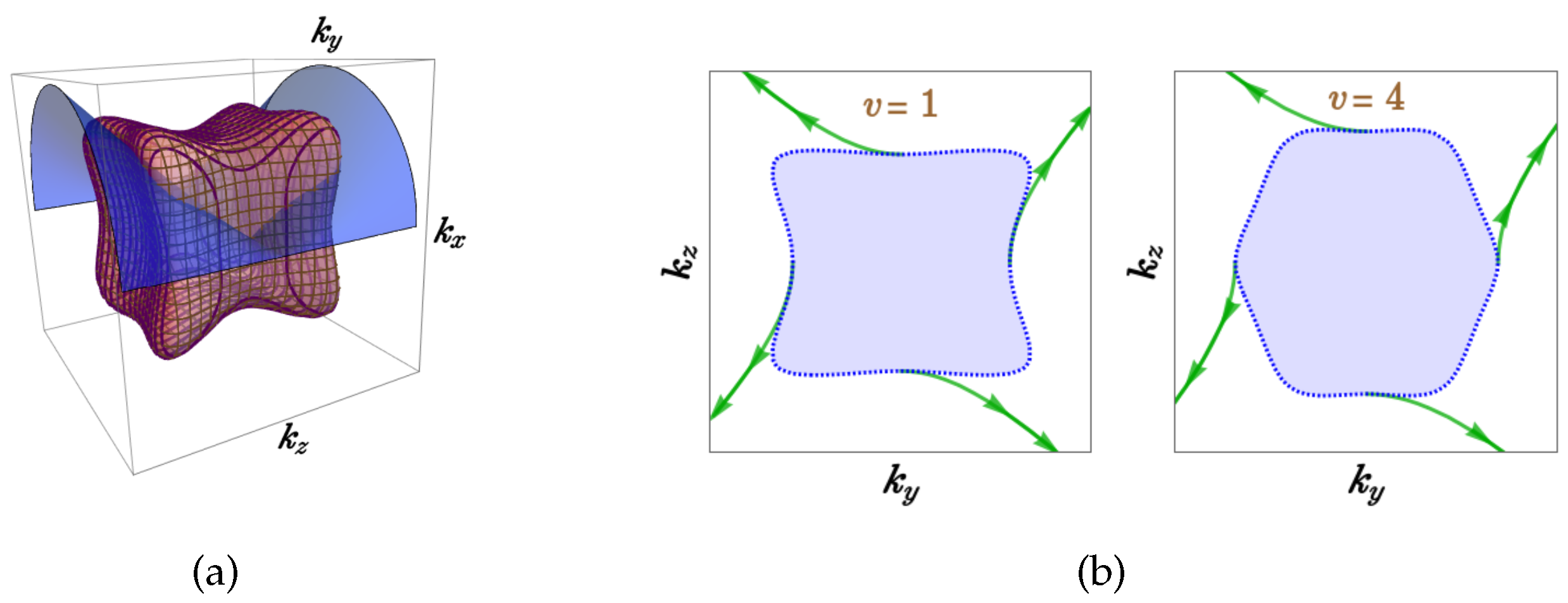
A quadruple-Weyl node (QWN) with twofold degeneracy carries [59,60,61,62] and can exist only in spinless systems at specific time-reversal symmetric points. Thus, they can appear in electronic bandstructures of materials with negligible SOC-couplings or in the phonon spectra of artificial crystals (such as photonic crystals), all of which can be treated as spinless systems. Let us take the lattice model of Ref. [62], where two nodes of opposite chiralities emerge at the - and R-points. For the node sitting at the -point can be described by the Hamiltonian, , where . The dispersion is cubic along the direction and quadratic along any other axis. On using , Eq. (6) yields the admissible solutions for are: (1) , , , , and ; and (2) , , , , and . Figure 4 illustrates a Fermi surface in 3d BZ as well as the arcs in the SBZ for , reflecting .
We have outlined how one can generically compute surface states in 3d topological semimetals. Through explicit examples, we have shown how the Fermi arc(s) reflect the net Chern number at a given NP, conforming to the well-established notion of bulk-boundary correspondence. Immediate future directions involve deciphering the dynamics of the Frmi arcs in the unconventional NPs studied here, which include nature of quantum oscillations [63,64].
Data Availability Statement
The data that support the findings of this study are available within the article.
References
- Burkov, A. A.; Balents, L. Phys. Rev. Lett. 2011, 107, 127205. [CrossRef] [PubMed]
- Hosur, P. Phys. Rev. B 2012, 86, 195102. [CrossRef]
- Armitage, N. P.; Mele, E. J.; Vishwanath, A. Rev. Mod. Phys. 2018, 90, 015001. [CrossRef]
- Hosur, P.; Qi, X. Comptes Rendus Physique 2013, 14, 857. [CrossRef]
- Yan, B.; Felser, C. Annual Rev. of Condensed Matter Phys. 2017, 8, 337. [CrossRef]
- Mandal, I.; Saha, K. Ann. Phys. (Berlin) 2024, 536, 2400016. [CrossRef]
- Bradlyn, B.; Cano, J.; Wang, Z.; Vergniory, M. G.; Felser, C.; Cava, R. J.; Bernevig, B. A. Science 2016, 353. [CrossRef]
- Fang, C.; Gilbert, M. J.; Dai, X.; Bernevig, B. A. Phys. Rev. Lett. 2012, 108, 266802. [CrossRef]
- Flicker, F.; de Juan, F.; Bradlyn, B.; Morimoto, T.; Vergniory, M. G.; Grushin, A. G. Phys. Rev. B 2018, 98, 155145. [CrossRef]
- Balduini, F.; Molinari, A.; Rocchino, L.; Hasse, V.; Felser, C.; Sousa, M.; Zota, C.; Schmid, H.; Grushin, A. G.; Gotsmann, B. Nature Communications 2024, 15, 6526. [CrossRef]
- Liang, L.; Yu, Y. Phys. Rev. B 2016, 93, 045113. [CrossRef]
- Isobe, H.; Fu, L. Phys. Rev. B 2016, 93, 241113.
- Tang, P.; Zhou, Q.; Zhang, S.-C. Phys. Rev. Lett. 2017, 119, 206402. [CrossRef]
- Ma, J.-Z.; Wu, Q.-S.; Song, M.; Zhang, S.-N.; Guedes, E.; Ekahana, S.; Krivenkov, M.; Yao, M.; Gao, S.-Y.; Fan, W.-H. Nature Communications 2021, 12, 3994. [PubMed]
- Shen, Y.; Jin, Y.; Ge, Y.; Chen, M.; Zhu, Z. Phys. Rev. B 2023, 108, 035428.
- Ghosh, R.; Haidar, F.; Mandal, I. Phys. Rev. B 2024, 110, 245113. [CrossRef]
- Mandal, I.; Saha, S.; Ghosh, R. Solid State Communications 2025, 397, 115799. [CrossRef]
- Mandal, I. arXiv e-prints [cond-mat.mes-hall. 2025a, arXiv:2506.12380.
- Xiao, D.; Chang, M.-C.; Niu, Q. Rev. Mod. Phys. 2010, 82, 1959.
- Sundaram, G.; Niu, Q. Phys. Rev. B 1999, 59, 14915. [CrossRef]
- Graf, A.; Piéchon, F. Phys. Rev. B 2021, 104, 085114.
- Zhuang, Z.-Y.; Zhang, C.; Wang, X.-J.; Yan, Z. Phys. Rev. B 2024, 110, L121122.
- Graf, A.; Piéchon, F. Phys. Rev. B 2023, 108, 115105.
- Habe, T. Phys. Rev. B 2022, 106, 205204.
- Ahn, S. Journal of the Korean Physical Society 2024, 84, 59.
- Xu, S.-Y.; Belopolski, I.; Alidoust, N.; Neupane, M.; Bian, G.; Zhang, C.; Sankar, R.; Chang, G.; Yuan, Z.; Lee, C.-C.; Huang, S.-M.; Zheng, H.; Ma, J.; Sanchez, D. S.; Wang, B.; Bansil, A.; Chou, F.; Shibayev, P. P.; Lin, H.; Jia, S.; Hasan, M. Z. Science 2015, 349, 613. [CrossRef]
- Lv, B. Q.; Weng, H. M.; Fu, B. B.; Wang, X. P.; Miao, H.; Ma, J.; Richard, P.; Huang, X. C.; Zhao, L. X.; Chen, G. F.; Fang, Z.; Dai, X.; Qian, T.; Ding, H. Phys. Rev. X 2015, 5, 031013.
- Sanchez, D. S.; Belopolski, I.; Cochran, T. A.; Xu, X.; Yin, J.-X.; Chang, G.; Xie, W.; Manna, K.; Süß, V.; Huang, C.-Y.; Alidoust, N.; Multer, D.; Zhang, S. S.; Shumiya, N.; Wang, X.; Wang, G.-Q.; Chang, T.-R.; Felser, C.; Xu, S.-Y.; Jia, S.; Lin, H.; Hasan, M. Zahid. Nature 2019, 567, 500–505. [CrossRef]
- Takane, D.; Wang, Z.; Souma, S.; Nakayama, K.; Nakamura, T.; Oinuma, H.; Nakata, Y.; Iwasawa, H.; Cacho, C.; Kim, T.; Horiba, K.; Kumigashira, H.; Takahashi, T.; Ando, Y.; Sato, T. Phys. Rev. Lett. 2019, 122, 076402. [CrossRef] [PubMed]
- Schröter, N. B. M.; Stolz, S.; Manna, K.; de Juan, F.; Vergniory, M. G.; Krieger, J. A.; Pei, D.; Schmitt, T.; Dudin, P.; Kim, T. K.; Cacho, C.; Bradlyn, B.; Borrmann, H.; Schmidt, M.; Widmer, R.; Strocov, V. N.; Felser, C. Science 2020, 369, 179.
- Yao, M.; Manna, K.; Yang, Q.; Fedorov, A.; Voroshnin, V.; Schwarze, B. Valentin; Hornung, J.; Chattopadhyay, S.; Sun, Z.; Guin, S. N.; Wosnitza, J.; Borrmann, H.; Shekhar, C.; Kumar, N.; Fink, J.; Sun, Y.; Felser, C. Nature Communications 2020, 11, 2033.
- Chang, G.; Xu, S.-Y.; Wieder, B. J.; Sanchez, D. S.; Huang, S.-M.; Belopolski, I.; Chang, T.-R.; Zhang, S.; Bansil, A.; Lin, H.; Hasan, M. Z. Phys. Rev. Lett. 2017a, 119, 206401.
- Xiao, X.; Jin, Y.; Ma, D.-S.; Kong, W.; Fan, J.; Wang, R.; Wu, X. Phys. Rev. B 2023, 108, 075130. [CrossRef]
- Witten, E. Riv. Nuovo Cim. 2016, 39, 313.
- Hashimoto, K.; Kimura, T.; Wu, X. Progress of Theoretical and Experimental Physics 2017, 053I01 (2017).
- Seradjeh, B.; Vennettilli, M. Phys. Rev. B 2018, 97, 075132. [CrossRef]
- Wawrzik, D.; You, J.-S.; Facio, J. I.; van den Brink, J.; Sodemann, I. Phys. Rev. Lett. 2021, 127, 056601. [PubMed]
- Okugawa, R.; Murakami, S. Phys. Rev. B 2014, 89, 235315. [CrossRef]
- Liu, Y.; Lin, J.; Wang, V.; Nara, J. Phys. Scripta [cond-mat.mes-hall]. 2025, arXiv:2107.11044100, 025939. [CrossRef]
- Faraei, Z.; Farajollahpour, T.; Jafari, S. A. Phys. Rev. B 2018, 98, 195402.
- Juergens, S.; Trauzettel, B. Phys. Rev. B 2017, 95, 085313. [CrossRef]
- Kharitonov, M.; Mayer, J.-B.; Hankiewicz, E. M. Phys. Rev. Lett. 2017, 119, 266402. [CrossRef]
- Zhu, Z.; Winkler, G. W.; Wu, Q.; Li, J.; Soluyanov, A. A. Phys. Rev. X 2016, 6, 031003.
- Sekh, S.; Mandal, I. Eur. Phys. J. Plus 137, 736 2022.
- Haidar, F.; Mandal, I. Annals of Physics 2025, 478, 170010. [CrossRef]
- Mandal, I. arXiv e-prints (2025b). arXiv [cond-mat.mes-hall. arXiv:2505.19636.
- Mandal, I. Phys. Rev. B 2025a, 111, 165116. [CrossRef]
- Chang, G.; Xu, S.-Y.; Wieder, B. J.; Sanchez, D. S.; Huang, S.-M.; Belopolski, I.; Chang, T.-R.; Zhang, S.; Bansil, A.; Lin, H.; Hasan, M. Z. Phys. Rev. Lett. 2017b, 119, 206401. [CrossRef] [PubMed]
- Xu, G.; Weng, H.; Wang, Z.; Dai, X.; Fang, Z. Phys. Rev. Lett. 2011, 107, 186806. [CrossRef]
- Huang, S.-M.; Xu, S.-Y.; Belopolski, I.; Lee, C.-C.; Chang, G.; Chang, T.-R.; Wang, B.; Alidoust, N.; Bian, G.; Neupane, M.; Sanchez, D.; Zheng, H.; Jeng, H.-T.; Bansil, A.; Neupert, T.; Lin, H.; Hasan, M. Z. Proceedings of the National Academy of Sciences 2016, 113, 1180. [CrossRef]
- Singh, B.; Chang, G.; Chang, T.-R.; Huang, S.-M.; Su, C.; Lin, M.-C.; Lin, H.; Bansil, A. Sci. Rep. 2018, 8, 10540. [PubMed]
- Fu, L. X.; Wang, C. M. Phys. Rev. B 2022, 105, 035201.
- Ghosh, R.; Mandal, I. Physica E: Low-dimensional Systems and Nanostructures 2024a, 159, 115914.
- Medel, L.; Ghosh, R.; Martín-Ruiz, A.; Mandal, I. Sci. Rep. 2024, 14, 21390.
- Mandal, I. Annals of Physics 2025b, 482, 170181.
- Chen, Q.; Fiete, G. A. Phys. Rev. B 2016, 93, 155125.
- Liu, Q.; Zunger, A. Phys. Rev. X 2017, 7, 021019.
- Ghosh, R.; Mandal, I. Journal of Physics: Condensed Matter 2024b, 36, 275501.
- Zhang, T.; Takahashi, R.; Fang, C.; Murakami, S. Phys. Rev. B 2020, 102, 125148.
- Cui, C.; Li, X.-P.; Ma, D.-S.; Yu, Z.-M.; Yao, Y. Phys. Rev. B 2021, 104, 075115.
- Luo, L.; Deng, W.; Yang, Y.; Yan, M.; Lu, J.; Huang, X.; Liu, Z. Phys. Rev. B 2022, 106, 134108. [CrossRef]
- Raj, A.; Chaudhary, S.; Fiete, G. A. Phys. Rev. Res. 2024, 6, 013048. [CrossRef]
- Potter, A. C.; Kimchi, I.; Vishwanath, A. Nature Communications 2014, 5, 5161. [CrossRef] [PubMed]
- Zhang, Y.; Bulmash, D.; Hosur, P.; Potter, A. C.; Vishwanath, A. Sci. Rep. 2016, 6, 23741. [CrossRef]
Figure 1.
(a) Dispersion (E) of the bands, crossing at a tilted Weyl node and a fourfold-degenerate Rarita-Schwinger-Weyl node, against the -plane. (b) Schematics of BC-flux field in the 3d momentum space for a monopole and an ideal dipole.
Figure 1.
(a) Dispersion (E) of the bands, crossing at a tilted Weyl node and a fourfold-degenerate Rarita-Schwinger-Weyl node, against the -plane. (b) Schematics of BC-flux field in the 3d momentum space for a monopole and an ideal dipole.
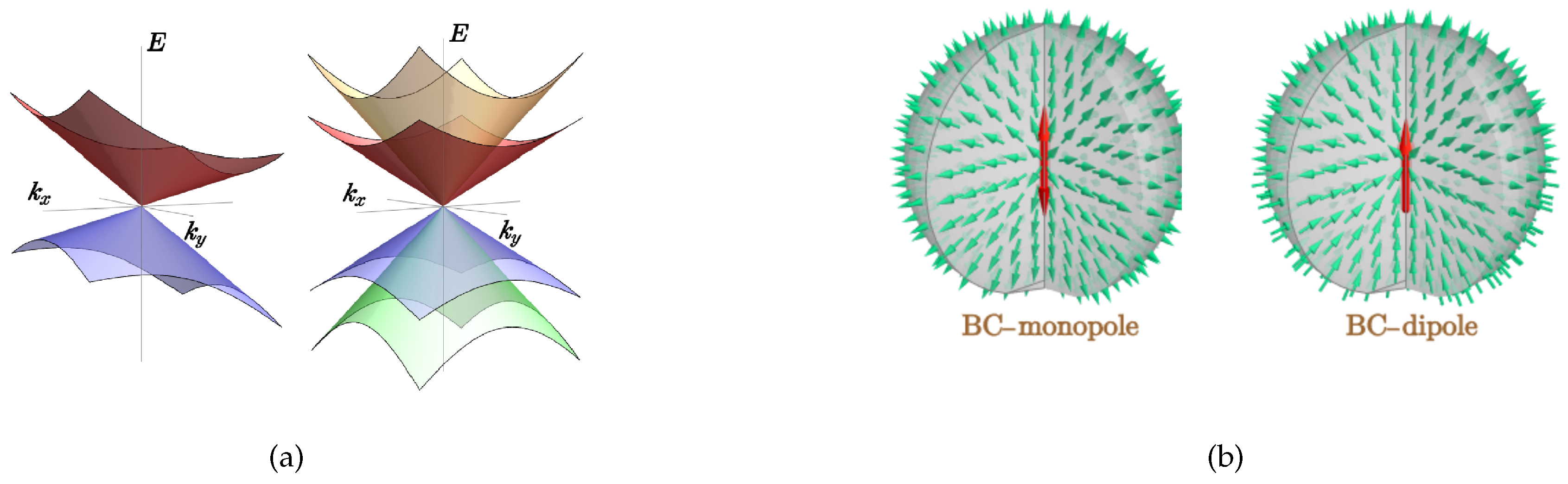
Figure 2.
(a) Tilted Weyl node with : Each Fermi arc corresponds to a distinct value of , colour-coded as shown in the plot-legends. (b) TSM node: 2 Fermi arcs entering into FS-projection. (c) RSW node: 4 Fermi arcs entering into the FS-projections. The dashed circles represent the projections of the bulk FSs with .
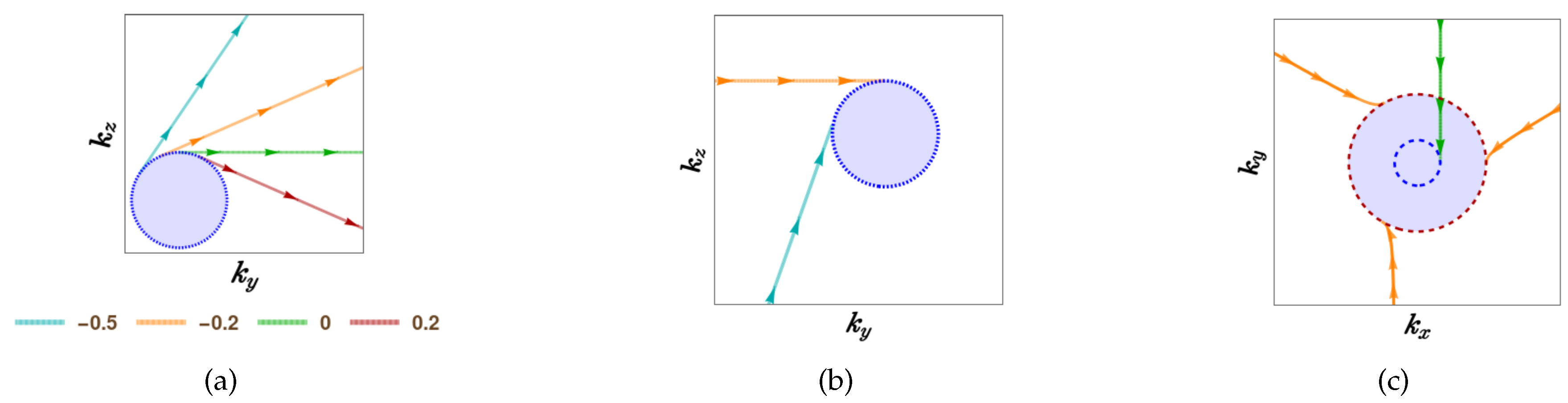
Figure 3.
(a) Double-Weyl node: 2 Fermi arcs leaving from the FS-projection. (b) Triple-Weyl node: 3 Fermi arcs leaving from the FS-projection. (c) and (d) represent the models with BC-dipole with two and three bands, respectively. In subfigure (d), arcs for 4 distinct values of have been shown.
Figure 3.
(a) Double-Weyl node: 2 Fermi arcs leaving from the FS-projection. (b) Triple-Weyl node: 3 Fermi arcs leaving from the FS-projection. (c) and (d) represent the models with BC-dipole with two and three bands, respectively. In subfigure (d), arcs for 4 distinct values of have been shown.
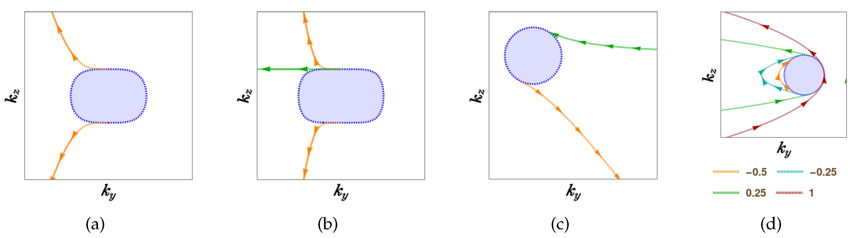
Figure 4.
(a) The FS-projection is obtained by cutting the 3d FS with the yellow-coloured 2d surface. Here, and . (b) The Fermi arcs represent modes with , emanating from the FS-projection (dashed closed curve) on the -plane.
Figure 4.
(a) The FS-projection is obtained by cutting the 3d FS with the yellow-coloured 2d surface. Here, and . (b) The Fermi arcs represent modes with , emanating from the FS-projection (dashed closed curve) on the -plane.
Disclaimer/Publisher’s Note: The statements, opinions and data contained in all publications are solely those of the individual author(s) and contributor(s) and not of MDPI and/or the editor(s). MDPI and/or the editor(s) disclaim responsibility for any injury to people or property resulting from any ideas, methods, instructions or products referred to in the content. |
© 2026 by the authors. Licensee MDPI, Basel, Switzerland. This article is an open access article distributed under the terms and conditions of the Creative Commons Attribution (CC BY) license (http://creativecommons.org/licenses/by/4.0/).
Copyright: This open access article is published under a Creative Commons CC BY 4.0 license, which permit the free download, distribution, and reuse, provided that the author and preprint are cited in any reuse.


