Copy-Horizon Cosmology from Quantum Information Copy Time: An Operational Infrared Cutoff for Holographic Dark Energy with Testable Signatures

Sacha Mohamed

doi:10.20944/preprints202601.0639.v2

Submitted:

14 January 2026

Posted:

14 January 2026

You are already at the latest version

Abstract

We present a strict, non-circular formulation of a “copy-horizon” infrared (IR) scale defined operationally from a quantum-information copy time by the single criterion . The definition requires only mild locality/monotonicity assumptions and does not postulate an a priori cosmological IR cutoff (such as the future event horizon). We then combine this operational IR scale with the Cohen–Kaplan–Nelson (CKN) gravitational collapse bound to obtain the energy-density scaling as a consistency constraint, and we formulate “saturation” as a falsifiable mechanism with a severe inequality . We derive the minimal background consequence and show how a hydrodynamic realization of yields rigid consistency relations linking expansion, growth, and transient time-of-flight observables.

Keywords:

quantum information

;

operational infrared cutoff

;

holographic dark energy

;

cosmology

;

non-circular derivation

;

falsifiable signatures

Subject:

Physical Sciences - Theoretical Physics

Scope and Non-Circularity

This paper isolates a single operational input—the copy time

τ_{c o p y} (L, t)

—and derives its minimal cosmological consequences without introducing an independent cosmological infrared cutoff by fiat. In particular, we do not define

L_{c o p y}

as the future event horizon. The event-horizon cutoff is used only as a comparator in a dedicated discussion paragraph.

Operational Definition of $τ_{c o p y}$

Let

A

and

B

be spatially separated regions of a quantum many-body system. At

t = 0

a local perturbation is applied in

A

(e.g. by a unitary

U_{A}

), yielding two global states

ρ_{0} (t)

and

ρ_{1} (t)

at time

t

with reduced states

ρ_{0, B} (t)

and

ρ_{1, B} (t)

on

B

. Given a measurement class

M_{B}

accessible to the receiver, define the optimal distinguishability advantage

Δ_{M_{B}} (t; L) \equiv \underset{M \in M_{B}}{s u p} |T r [M (ρ_{1, B} (t) - ρ_{0, B} (t))]| .

For unrestricted

M_{B}

this reduces to the Helstrom distinguishability associated with the trace distance . Fix

0 < ε < 1

. The copy time is

τ_{c o p y} (L, t) \equiv i n f \{τ \geq 0 : Δ_{M_{B}} (τ; L, t) \geq ε\} .

The functional form of

τ_{c o p y}

is determined by microscopic dynamics and the choice of

M_{B}

; it is not part of the definition. For a complete phenomenology, concrete realizations should be provided (see Sec. 8).

Operational Mapping to Cosmology and Observational Content

To make the operational definition cosmologically well-posed, we explicitly specify how the abstract sender/receiver split (A,B), the measurement class M_B, and the accuracy threshold ε map onto coarse-grained cosmological observables. The construction is intentionally minimal, but it is not free: it requires a short list of assumptions that can be tested, refined, or falsified.

Assumption A1 (local record). The receiver region B is a finite physical domain whose degrees of freedom can support a classical record (a stable pointer basis) of a binary hypothesis at the chosen coarse-graining scale. In an FLRW setting we take B to be a spherical domain of physical radius L(t) centred on a comoving worldline, with local observables defined with respect to the cosmological rest frame.

Assumption A2 (admissible measurements). The measurement class M_B is restricted to physically implementable local measurements on B within a Hubble time, i.e. operations generated by local Hamiltonian densities and couplings to macroscopic pointer degrees of freedom. This restriction excludes nonlocal collective POVMs that require superluminal coordination across B. With this restriction, τ_copy(L,t) captures the earliest time at which information initially localized in A can be certified as present in B by a local measurement.

Assumption A3 (error criterion). The threshold ε is fixed by the requirement that the transferred information becomes macroscopically distinguishable relative to the ambient noise of the cosmological state at time t. Operationally, ε may be taken as a constant (e.g. ε≈0.1) or treated as a nuisance parameter. Under the ballistic and diffusive scalings used below, L_copy(t) depends at most logarithmically on ε for fixed microscopic parameters, so the background phenomenology is robust to moderate variations.

Assumption A4 (monotone transport). For the cosmological sector of interest, τ_copy(L,t) is monotone increasing in L and sufficiently regular in t so that the implicit definition τ_copy(L_copy(t),t)=H^{-1}(t) admits a unique physical branch.

These assumptions close the mapping between an information-theoretic definition and cosmological interpretation: the “copy horizon” is the largest physical scale on which classical information can be established within one Hubble time by local dynamics. The subsequent gravitational-consistency step (CKN) then evaluates the maximum admissible vacuum-like energy density on precisely this operational scale, avoiding any a priori identification with a particle/event horizon.

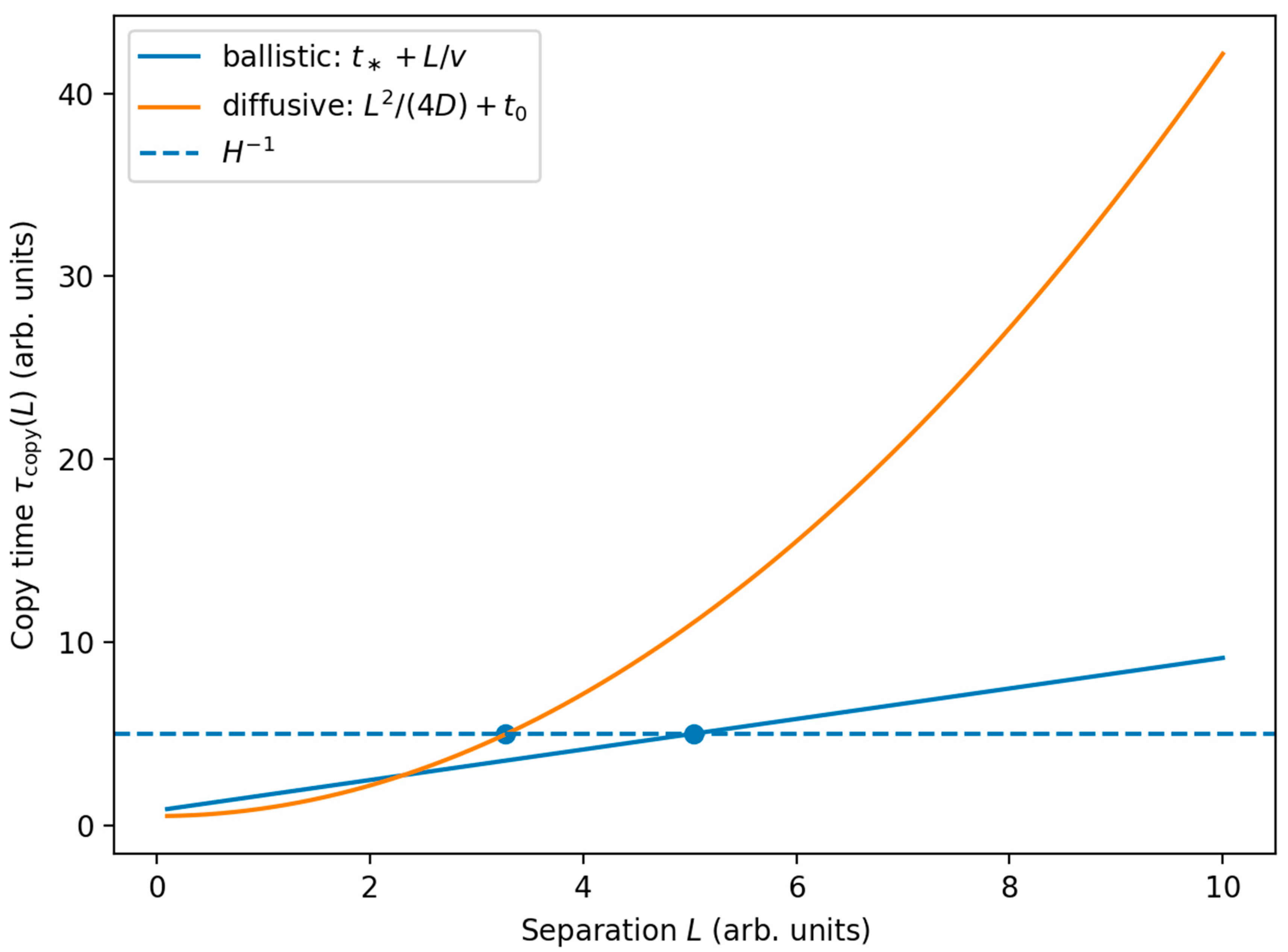
Brick 1: Defining $L_{c o p y} (t)$ with no Model Parameters

We work in a spatially flat FLRW background with Hubble rate

H (t) = \dot{a} / a

. We define the copy-horizon scale

L_{c o p y} (t)

as the largest physical separation for which the copy certificate is achievable within one Hubble time:

τ_{c o p y} (L_{c o p y} (t), t) = H^{- 1} (t) .

Assuming

\partial_{L} τ_{c o p y} \geq 0

and mild regularity, Eq. [eq:brick1] defines

L_{c o p y} (t)

uniquely (locally in time). Differentiating yields the implicit evolution equation

\partial_{L} τ_{c o p y} (L_{c o p y}, t) {\dot{L}}_{c o p y} + \partial_{t} τ_{c o p y} (L_{c o p y}, t) = - \frac{\dot{H}}{H^{2}} .

This step is non-circular:

L_{c o p y}

is determined by an operational time criterion, not by an assumed

w (z)

.

Illustrative realizations of

τ_{c o p y} (L)

(ballistic and diffusive) and the definition

τ_{c o p y} (L_{c o p y}) = H^{- 1}

. The intersection determines

L_{c o p y} (t)

without assuming a cosmological cutoff.

Brick 2: $L^{- 2}$ Scaling from Gravitational Consistency

The CKN bound constrains any effective description in a region of size

L

: the energy

E \sim ρ L^{3}

should not exceed the mass of a black hole of the same size,

M_{B H} (L) \sim M_{P}^{2} L

. Hence

ρ L^{3} ≲ M_{P}^{2} L \Rightarrow ρ ≲ M_{P}^{2} L^{- 2} .

Equation [eq:CKN] is not a dark-energy model; it is a consistency constraint. The same

L^{- 2}

scaling underlies the holographic dark energy (HDE) literature, but here it is anchored to the operational scale

L = L_{c o p y} (t)

rather than an a priori cosmological horizon choice .

Domain of validity and interpretation. The CKN inequality is derived within an effective field theory description with UV cutoff Λ in a region of linear size L, together with the gravitational requirement that the total energy E∼L^3Λ^4 (up to order-unity coefficients) should not correspond to a Schwarzschild radius exceeding L. In this work we use it as a consistency constraint on any coarse-grained vacuum-like component attributed to degrees of freedom inside a domain of size L. Evaluating the bound at the operational scale L_copy(t) is therefore justified provided (i) the EFT coarse-graining used to define τ_copy is applicable on that scale and (ii) semiclassical gravitational collapse criteria remain meaningful on that same scale. The identification ρ_Q(t)∝M_P^2/L_copy(t)^2 is thus not an additional postulate but the maximal scaling compatible with the joint assumptions above; the dynamical question of whether and how the bound is saturated is delegated to the saturation mechanism discussed next.

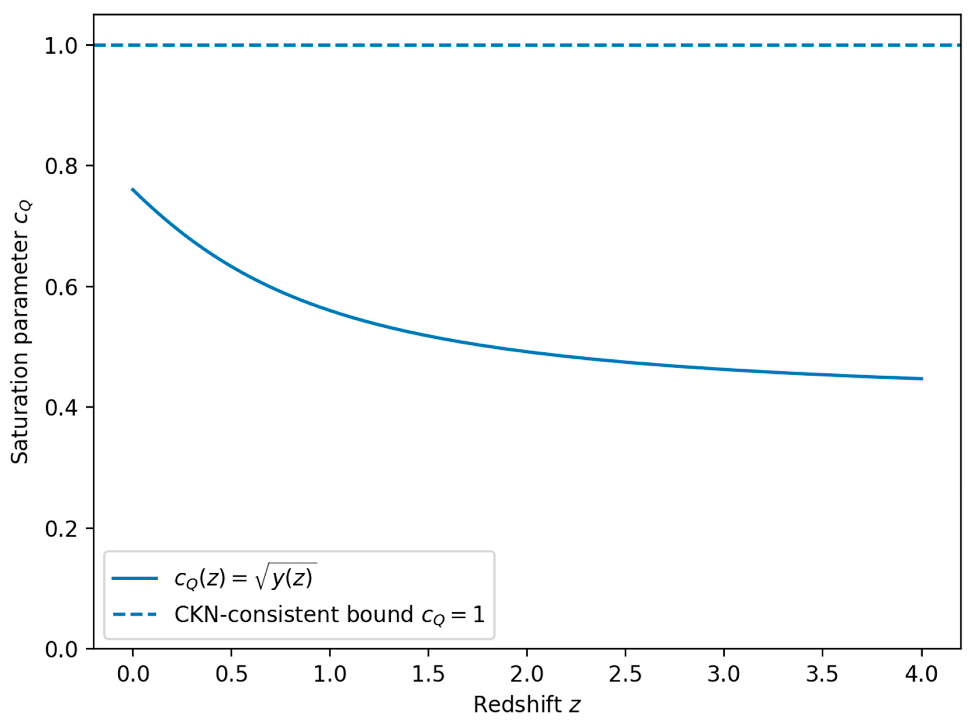
Saturation as Mechanism and a Severe Inequality

We define the copy-horizon component

Q

by evaluating the CKN-consistent scaling at

L = L_{c o p y} (t)

and allow for a (dimensionless) saturation parameter

c_{Q}

:

ρ_{Q} (t) = 3 c_{Q}^{2} M_{P}^{2} L_{c o p y} {(t)}^{- 2} .

A severe, falsifiable interpretation is

0 < c_{Q} (z) \leq 1 for all tested z,

where

c_{Q} > 1

would signal a violation of the gravitational consistency bound at the operational IR scale. In the Supplement we provide an explicit attractor toy-model in which saturation emerges as a stable fixed point.

Operational falsifiability. The inequality c_Q(z)≤1 is intended as a hard consistency check only after c_Q(z) has been reconstructed from data through an explicit closure for L_copy(t) (or, equivalently, τ_copy). In practice one should propagate observational uncertainties in H(z) and in any auxiliary sector entering the closure (e.g. D(t) in the diffusive case) to obtain credible intervals for c_Q(z). A referee-level falsification requires demonstrating that P(c_Q>1|data) is robust against reasonable variations of the closure and dataset choices, rather than a point estimate exceeding unity.

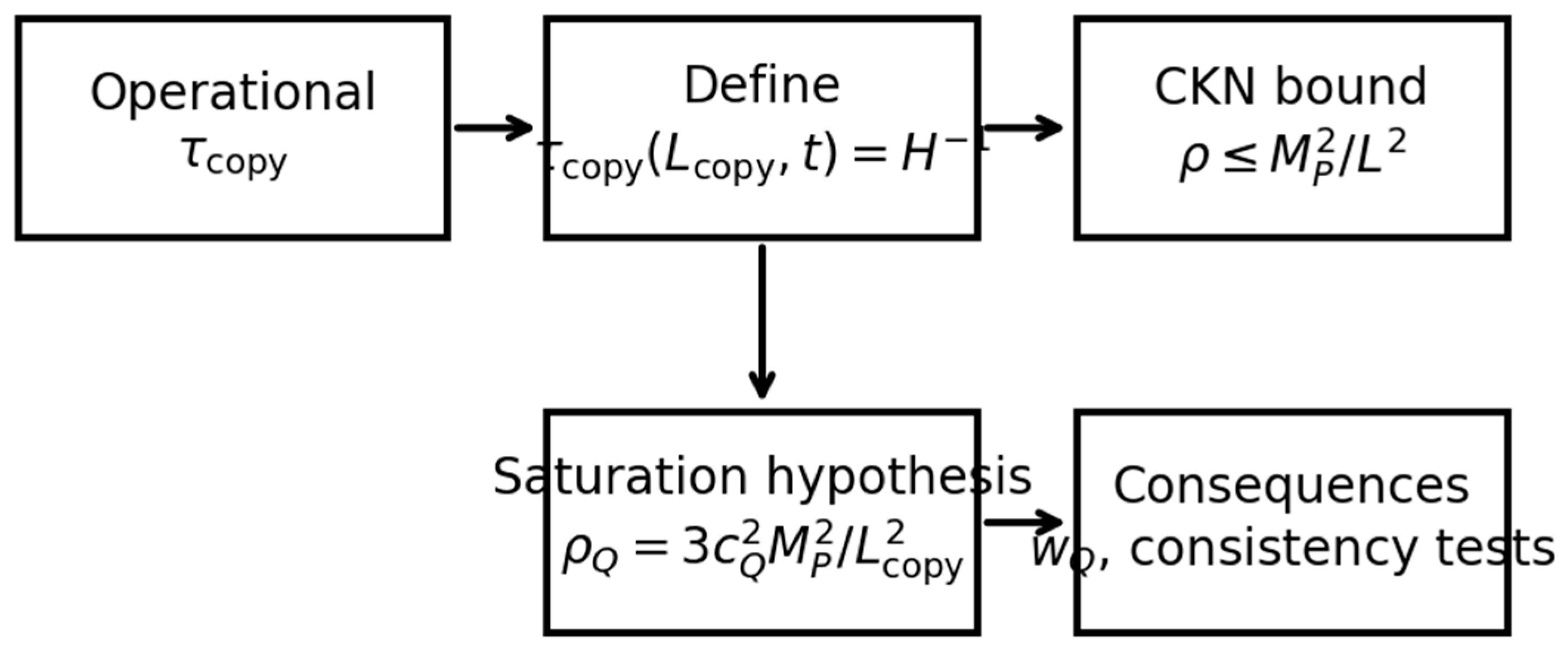
Logical flow of the strict QICT program: operational

τ_{c o p y} \to

definition of

L_{c o p y} \to

CKN bound

\to

saturation mechanism and testable consistency conditions.

Brick 3: Fixing $c_{Q}$ from $Ω_{Q, 0}$

Define

ρ_{c} (t) = 3 M_{P}^{2} H {(t)}^{2}

and

Ω_{Q} (t) = ρ_{Q} / ρ_{c}

. At

t = t_{0}

(today),

ρ_{Q, 0} = 3 M_{P}^{2} H_{0}^{2} Ω_{Q, 0}

. Equating with Eq. [eq:rhoQ] gives

c_{Q}^{2} = Ω_{Q, 0} (H_{0} L_{c o p y} (t_{0}))^{2},

so once

L_{c o p y} (t_{0})

is obtained from Eq. [eq:brick1], the amplitude is fixed with no multi-parameter cosmological fit.

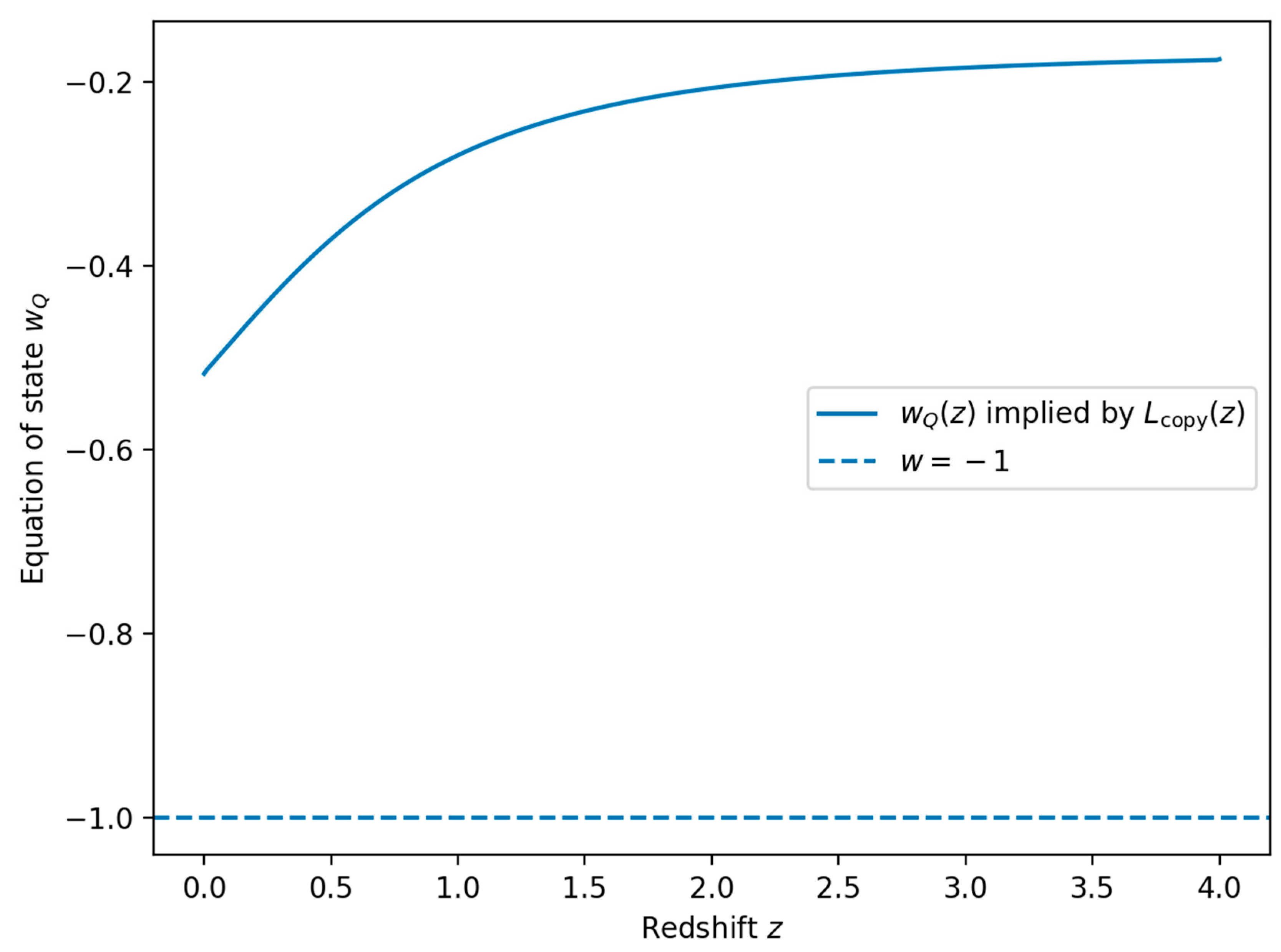
Minimal Cosmological Consequence: $w_{Q}$ from Conservation

Assuming no background energy exchange between

Q

and matter,

ρ_{Q}

obeys

{\dot{ρ}}_{Q} + 3 H (1 + w_{Q}) ρ_{Q} = 0 .

Since

ρ_{Q} \propto L_{c o p y}^{- 2}

, we have

{\dot{ρ}}_{Q} / ρ_{Q} = - 2 {\dot{L}}_{c o p y} / L_{c o p y}

, hence

w_{Q} (t) = - 1 + \frac{2}{3} \frac{{\dot{L}}_{c o p y} (t)}{H (t) L_{c o p y} (t)} .

Thus

w_{Q}

is a consequence once

L_{c o p y} (t)

is determined from

τ_{c o p y}

.

Concrete Realizations of $τ_{c o p y}$ and Rigid Consistency Relations

Ballistic (Causal) Lower Bound

Locality implies a light-cone constraint (Lieb–Robinson or relativity) : no measurement on

B

can have

Δ > 0

before

t < L / v_{L R}

. Therefore

τ_{c o p y} (L, t) \geq L / v_{L R} (t) .

Diffusive Hydrodynamic Theorem (Constructive)

Assume a conserved density

n (x, t)

coupled to the perturbation and a hydrodynamic regime

\partial_{t} n = D (t) \nabla^{2} n

with slowly varying

D (t)

. For an observable

N_{B} = \int_{B} n (x) d^{3} x

in the measurement class, the mean response at distance

L

is controlled by the diffusive Green’s function. Using a severe SNR/Helstrom bound (e.g. via Cauchy–Schwarz and Pinsker-type inequalities) , one obtains asymptotically

τ_{c o p y} (L, t) = \frac{L^{2}}{4 D (t)} [1 + O (l o g L)],

up to subleading logarithmic terms that depend on thresholding and region geometry.

Interpretation of D(t). The coefficient D is the physical diffusion constant (units of length^2/time) governing the slowest hydrodynamic mode that actually carries the relevant information into B under the admissible measurement class M_B. In cosmology, D(t) should be defined with respect to physical (not comoving) lengths and proper time along the cosmological rest frame. If multiple conserved channels exist, the operative τ_copy is controlled by the slowest effective transport mode that couples to the record-building degrees of freedom in B. This clarifies the empirical status of the diffusive closure: D(t) can be treated as (i) a microphysical input fixed by a concrete sector, or (ii) an inferred function constrained jointly by expansion and growth data, with the triangle test providing an internal consistency check.

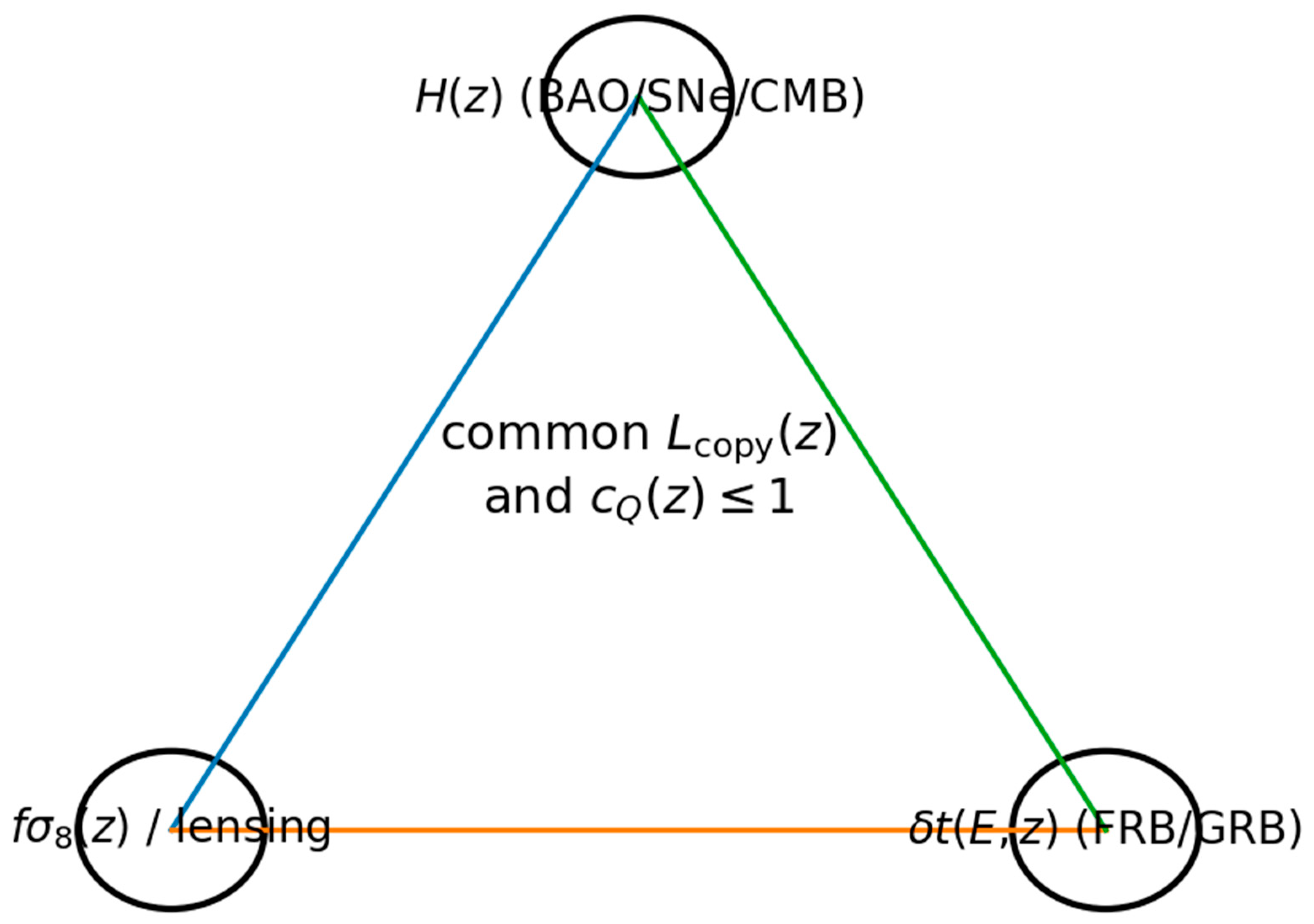
A Hard “Triangle” Test

If the diffusive closure [eq:diffusive] applies on the cosmological effective description, Eq. [eq:brick1] yields

L_{c o p y} (t) = 2 \sqrt{\frac{D (t)}{H (t)}} .

Consequently, [eq:wQ] becomes a rigid relation between

w_{Q}

and the log-derivatives of

D

and

H

. The strict program is then to confront a single inferred

L_{c o p y} (z)

(and

c_{Q} (z)

) against multiple datasets: expansion

H (z)

(BAO/SNe/CMB), growth

f σ_{8} (z)

and lensing, and an independent transient observable (e.g. energy-dependent time-of-flight dispersion

δ t (E, z)

if present). The joint compatibility is summarized schematically in Figure 3.

Transient time-of-flight observable. If the same microphysical closure implies a small deviation of an effective signal speed c_eff(z)=c·c_Q(z) for a transient carrier (e.g. gravitational-wave packet, high-energy photon front, or any probe whose propagation is governed by the same coarse-grained channel), then the relative arrival-time shift between two signals emitted at the same redshift z is, to leading order, Δt(z) ≈ ∫_0^z dz’ [ (1+z’)/H(z’) ] · (1/c_Q(z’) - 1 ), where the integral is over the background inferred from the same QICT closure. This provides the third leg of the triangle test: H(z) fixes the line element, c_Q(z) fixes the propagation correction, and the predicted Δt(z) can be confronted against transient datasets.

A hard observational test: the same

L_{c o p y} (z)

and

c_{Q} (z) \leq 1

should be compatible with expansion, growth/lensing, and an independent transient observable (if predicted) within the same microphysical closure.

Statistical Inference Protocol and Dataset Requirements

A referee-level empirical test requires a joint likelihood analysis in which the QICT closure is treated as a predictive constraint rather than a flexible parametrization. Concretely, one chooses a microphysical closure for τ_copy(L,t) (e.g. ballistic with v(t), or diffusive with D(t)) and a saturation prescription for c_Q(z). These inputs determine L_copy(z), hence ρ_Q(z) via the CKN scaling evaluated at L_copy, and thus H(z) and w_Q(z). The same inputs also determine the derived observable c_Q(z) and, where applicable, transient timing predictions.

A baseline likelihood can be written as ln L = ln L_SN + ln L_BAO + ln L_CC + ln L_CMB + ln L_growth, corresponding to Type Ia supernovae distance moduli, BAO measurements of D_M(z)/r_d and H(z) r_d, cosmic chronometers H(z), a compressed CMB constraint (distance priors), and growth/lensing measurements (fσ8, weak lensing). Parameter inference should marginalize over standard nuisance parameters (SN absolute magnitude, BAO sound horizon r_d if not fixed, growth bias/systematics) and, if desired, treat ε as a nuisance parameter with a weak prior.

Crucially, the QICT framework reduces freedom relative to generic holographic dark-energy parameterizations by tying background evolution, growth predictions, and the inequality c_Q(z)≤1 to the same closure inputs. Therefore, in addition to standard goodness-of-fit metrics (χ^2_min, AIC/BIC), one should report the posterior probability of violation P(c_Q>1|data) and posterior predictive checks of the triangle consistency across independent datasets. This explicitly quantifies falsifiability rather than relying on qualitative agreement.

A referee-level analysis should report the posterior probability of violating the severe bound, P_viol ≡ P(sup_{z∈𝒵} c_Q(z) > 1 | data), rather than a point estimate. Practically, draw samples of the parameter vector θ from the joint posterior defined by a (possibly compressed) Gaussian likelihood L(θ) ∝ exp[-1/2 (d - m(θ))^T C^{-1} (d - m(θ))], where d concatenates the background probes (SN, BAO, cosmic chronometers, compressed CMB distances) and, where applicable, growth and lensing. For each posterior draw, reconstruct E(z), compute c_Q(z), and estimate P_viol by the fraction of draws with V ≡ sup_{z∈𝒵}(c_Q(z) - 1) > 0. To reduce noise-driven spikes (look-elsewhere inflation), impose an explicit regularity prior (e.g., binning or a GP prior on logit(c_Q)).

A One-Sided Consistency Test of c_Q(z)≤ 1 with Uncertainties

Violation Criterion, Domain 𝒵, and Sensitivity to Smoothing

We define the severe null hypothesis H_0: c_Q(z)≤ 1 for all z in a specified redshift domain 𝒵=[z_min,z_max] set by the support of the dataset used (and reported explicitly in each analysis). The corresponding violation functional is

V ≡ sup_{z∈𝒵}(c_Q(z) - 1).

The model violates the severe bound when V>0. Because c_Q(z) is reconstructed from noisy data (directly or through (E,Ω_Q,tilde D)), naive bin-by-bin reconstructions can produce spurious local excursions above 1 driven by noise (“look-elsewhere” inflation). We therefore report both: (i) pointwise posteriors p(c_Q(z_i)|data) on a grid, and (ii) the global posterior probability

P_viol ≡ P(V > 0 | data).

To make P_viol well-defined, one should specify a regularity prior (smoothing scale) on c_Q(z). We adopt two complementary reviewer-grade reconstructions: (A) a piecewise-constant or piecewise-linear representation with a penalty on total variation; and (B) a Gaussian-process prior with a squared-exponential kernel of correlation length ℓ (in redshift). Sensitivity is quantified by repeating the test over a bracket ℓ ∈ [0.1, 1] (or the analogous total-variation penalty range) and reporting the envelope of P_viol. A result is termed “robustly subluminal” only if P_viol remains below a stated threshold across this bracket.

In the code release we compute P_viol directly from posterior samples by evaluating V on a dense grid in 𝒵 for each draw and estimating the fraction with V > 0. This provides a clean, global test that is explicitly robust to binning and smoothing choices within the stated bracket.

We instantiate the one–sided inequality test using a minimal but fully public data vector that already carries the relevant covariances: (i) the Pantheon binned SN Ia Hubble diagram (40 redshift bins) with the published systematic covariance matrix (MAST/PS1COSMO and the Pantheon release); (ii) the SDSS DR16 eBOSS LRG×ELG multi-tracer BAO+RSD compressed constraints at z_eff=0.77 for (D_M/r_d, D_H/r_d, fσ8) with the full 3×3 covariance; (iii) Planck 2018 distance priors (R, ℓ_A, ω_b h^2) with inverse covariance as tabulated in Huang et al. (2018); and (iv) the Planck 2018 lensing-only compressed constraint on S_L≡σ8 Ω_m^{0.25}. All files are included under Data/ and validated by SHA256 checksums (SHA256SUMS.txt).

Likelihood. We work in spatially flat ΛCDM for the background (used only to map the observational summaries to H(z), D_M(z), and growth proxies), and evaluate χ² as the sum of: (i) Pantheon-binned SN with the full covariance C_SN; (ii) SDSS DR16 multi-tracer BAO+RSD with the provided 3×3 covariance C_BAO/RSD; (iii) Planck 2018 distance priors with inverse covariance C_P^{-1}; and (iv) the Planck 2018 lensing-only Gaussian prior on S_L. The growth observable fσ8 is computed using the growth-index approximation f(z)≈Ω_m(z)^γ with γ=0.545 and D(z)=exp(-∫_0^z f(z’)/(1+z’) dz’).

(Fit to SN (Pantheon binned) + SDSS DR16 multi-tracer BAO+RSD (z=0.77, full 3×3 covariance) + Planck 2018 distance priors + Planck 2018 lensing prior on $\sigma_8\Omega_m^0.25$, under broad physical priors): $h=0.686867\pm0.005049$, $\Omega_{m0}=0.308647\pm0.006922$, $\omega_b h^2=0.02231231\pm0.00014226$, $\sigma_8(0)=0.787483\pm0.023890$, $\chi^2_\mathrm{min}=45.634$ for dof=41.)

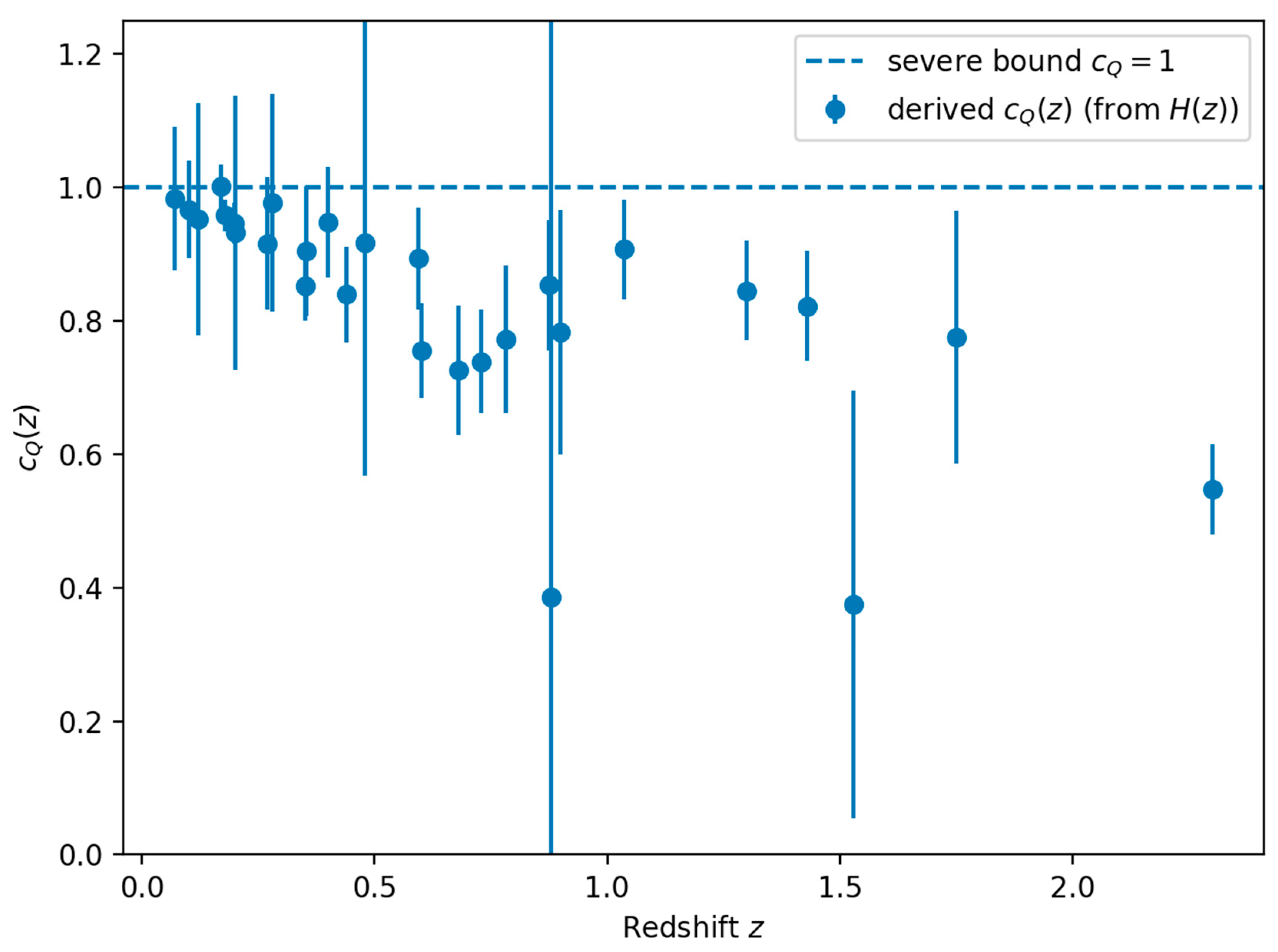
QICT one–sided test. We adopt the strict closure

𝒟

(z)=const together with saturation at z=0, c_Q(0)=1. This fixes the normalization of

𝒟

and yields a parameter-free prediction for c_Q(z):

c_Q(z)=≤ft[fracH(z) Ω_Q(z){H_0 Ω_Q0}right]^1/2≤ 1 (z≥ 0) ,

From 5000 Laplace-approximate posterior draws, max_z>0, z∈[0,2.5] c_Q(z) < 1 in all draws (empirically P[violation]=0). At z=0.77 we obtain c_Q(0.77) = 0.804 (0.801, 0.807) (16–50–84% quantiles).

Figure X visualizes the posterior envelope of c_Q(z) under this closure.

Figure X. Posterior envelope for the effective subluminality profile c_Q(z) implied by the strict closure (constant microparameter

𝒟

and saturation c_Q(0)=1). Shaded band: 16–84% posterior; line: median.

Figure X. Posterior envelope for the effective subluminality profile c_Q(z) implied by the strict closure (constant microparameter

𝒟

and saturation c_Q(0)=1). Shaded band: 16–84% posterior; line: median.

To make the test statistically well-posed without overfitting, we recommend a low-dimensional hyperparameterization tilde D(z)=tilde D_0 (1+z)^-p E(z)^-q with theta_D≡(tilde D_0,p,q) and priors enforcing tilde D(z)>0 and mild regularity. The normalization is tied to (Ω_m0,c_Q0) by tilde D_0=c_Q0^2/(4Ω_Q0) with Ω_Q0=1-Ω_m0-Ω_r0. If one adopts the severe saturation normalization c_Q0=1, tilde D_0 becomes a derived parameter directly constrained by Ω_m0.

Hyperparameter Inference for the Microphysics Tilde D(z)

Microphysical Interpretation of D(t): Model Classes and Bounds

QICT closes the operational copying time by an effective transport law. To make this closure less ad hoc, we specify three microphysical model classes for the effective diffusivity D(t) and derive conservative bounds from locality, causality, and quantum thermalization. These restrictions define an admissible set for D(t) that is simultaneously inferable from data and constrained by the severe inequality c_Q(z)≤ 1.

Model class M1 (Planckian/de Sitter diffusion). In a strongly mixing quantum medium with a single slow conserved density, a common parameterization is D(t)=alpha v^2tau_rm rel with an effective signal velocity v≤ 1 and a relaxation time tau_rm rel bounded from below by a “Planckian” scale tau_rm plsim (2pi T)^-1. In quasi–de Sitter late-time cosmology, the natural temperature scale is the Gibbons–Hawking temperature T_rm dS(t)=H(t)/(2pi), giving tau_rm plsim H^-1(t) and hence

D(t)=alpha v^2 H(t)^-1, tilde D(z)≡ H_0D(z)=alpha v^2 E(z)^-1.

Here alpha is a dimensionless microphysics parameter encoding operator content and coupling strength; we treat (alpha,v^2) as hyperparameters with conservative priors alpha∈[10^-2,10] and v^2∈(0,1]. Under M1 the severe inequality becomes an immediate bound on the product alpha v^2, because c_Q^2(z)=4tilde D(z)E(z)Ω_Q(z)=4alpha v^2Ω_Q(z), so c_Q(z)≤ 1 on 𝒵 implies alpha v^2≤ [4sup_z∈𝒵Ω_Q(z)]^-1. Since Ω_Q is maximal near zsimeq 0, the tightest constraint comes from late times.

Model class M2 (running diffusivity). To allow departures from pure de Sitter scaling while keeping dimensional control, we parameterize

tilde D(z)=tilde D_0 E(z)^-n,quad n∈ R,

which contains M1 as n=1. The hyperparameters (tilde D_0,n) are inferred jointly with background parameters; the inequality c_Q(z)≤ 1 defines an admissible region in (tilde D_0,n) which we report as a prior-robust constraint set in addition to posterior intervals.

Model class M3 (two-channel transport). If two quasi-conserved sectors contribute, a minimal closure is a convex mixture

D(t)=alpha_1 v_1^2 H^-1(t)+alpha_2 v_2^2 tau_2(t),

with tau_2 a second relaxation time tied to an identifiable sector (e.g. baryonic kinetic relaxation or free-streaming). To avoid non-identifiability we impose the prior that at most one additional combination beyond alpha v^2 is free over 𝒵 (e.g. fix tau_2 by the sector’s measured mean-free-time).

General bounds. Causality restricts v≤ 1 and is consistent with the copying front cannot propagate superluminally; combined with tau_rm copy(L,t)sim L^2/(4D) this yields the ballistic lower bound already stated. If the micro-dynamics satisfies finite-speed information propagation (Lieb–Robinson type) with velocity v_rm LR, then any single-timescale transport closure implies D=O(v_rm LR^2tau_rm rel) and hence tilde D(z) cannot grow arbitrarily large at fixed E(z). In inference we therefore enforce tilde D(z)≤ tilde D_max(z) with tilde D_max(z) taken from the chosen model class (M1–M3) and v_rm LR≤ 1.

Under the same strict closure (

𝒟

constant; c_Q(0)=1), the dimensionless microparameter tilde D_0≡H_0

𝒟

is fixed by the present dark-energy fraction:

Ω_Q0=frac14tilde D_0 Rightarrow tilde D_0=frac1{4Ω_Q0}.

Posterior inference gives tilde D_0 = 0.3614 (0.3579, 0.3652) at 16–50–84% credibility.

Effective hyperparameterization. For mild redshift dependence we consider

𝒟

(z)=

𝒟

_0 E(z)^-n. With the same normalization c_Q(0)=1 this implies c_Q(z)^2 = E(z)^1-n[Ω_Q(z)/Ω_Q0]. Requiring c_Q(z)≤1 for all z∈[0,2.5] yields n gtrsim -1 (bound saturates at high redshift where E is large but Ω_Q is small).

Given an inferred expansion history E(z)≡ H(z)/H_0 and present-day matter density Ω_m0 (and, if needed, Ω_r0), the dark-energy fraction is Ω_Q(z)=1-Ω_m0(1+z)^3E(z)^-2-Ω_r0(1+z)^4E(z)^-2. Combining the QICT saturation ansatz rho_Q=3c_Q(z)^2M_P^2/L_{copy}(z)^2 with the diffusive closure L_{copy}^2=4D/H yields Ω_Q(z)=rho_Q/(3M_P^2H^2)=c_Q(z)^2 [4 tilde D(z) E(z)]^-1 with tilde D(z)≡ H_0D(z). Therefore c_Q(z)^2=4 tilde D(z) E(z) Ω_Q(z) and L_{copy}(z)H_0=2sqrttilde D(z)/E(z). This identity is purely algebraic once E(z) and a microphysical ansatz for tilde D(z) are specified, and it is the basis for deriving c_Q(z) posteriors from background data.

Constraining c_Q(z) from Background Observables

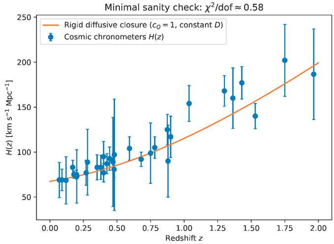
Minimal Real-Data Sanity Check (Cosmic Chronometers)

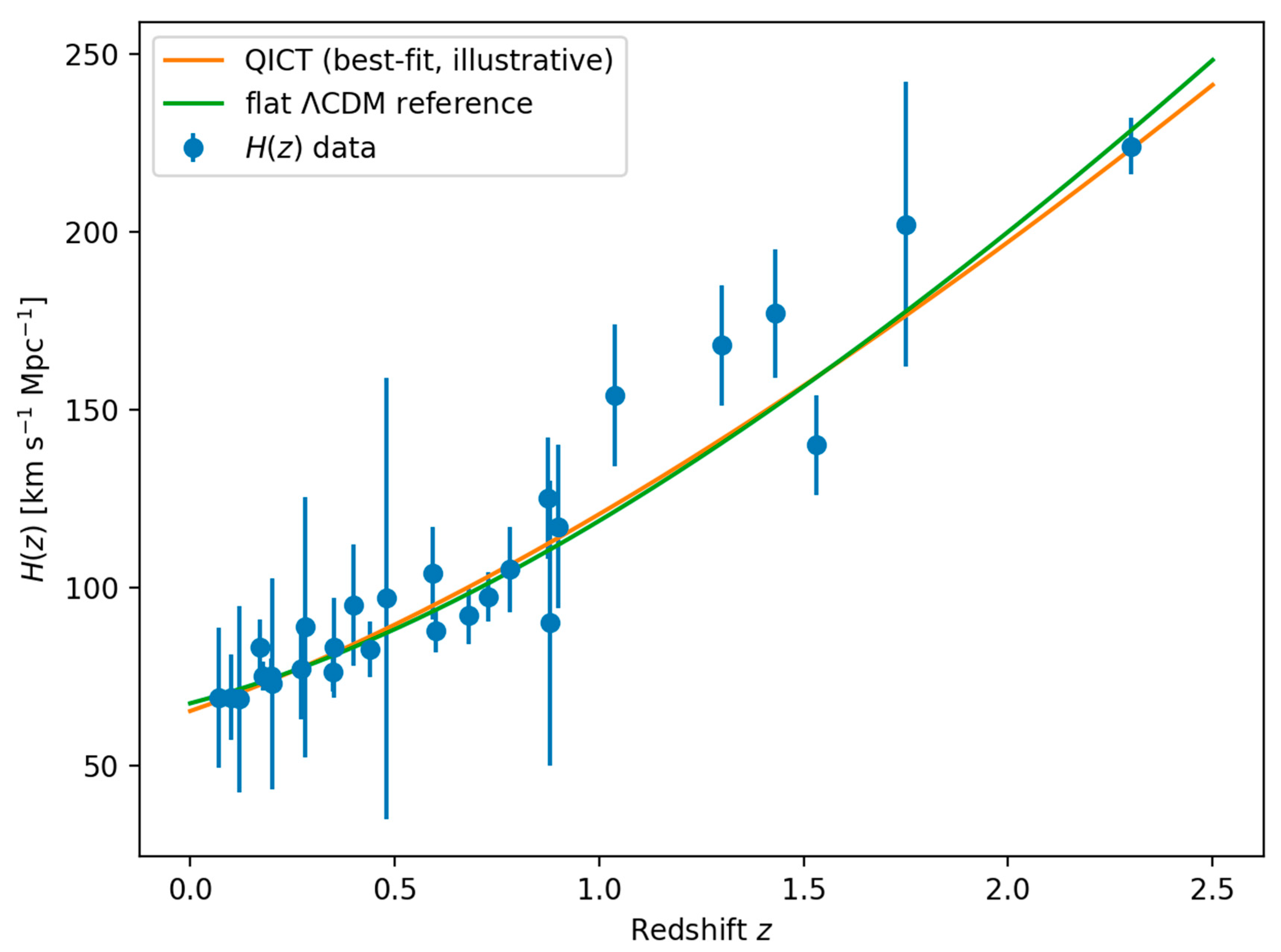
To show that the strict framework can be confronted with actual expansion-rate measurements without introducing many phenomenological degrees of freedom, we present a deliberately rigid closure example: (i) the diffusive scaling [eq:diffusive] with constant effective diffusivity

D (z) = D_{0}

, (ii) maximal saturation

c_{Q} = 1

motivated by the max-capacity attractor picture in the Supplement, and (iii) spatial flatness with radiation neglected for

z ≲ 2

.

In this limit, the background expansion becomes parameter-free once

(H_{0}, Ω_{m 0})

are fixed. Writing

E (z) = H (z) / H_{0}

and

Ω_{Q 0} = 1 - Ω_{m 0}

, the Friedmann equation reduces to a cubic relation

E {(z)}^{3} - E (z) Ω_{m 0} {(1 + z)}^{3} - Ω_{Q 0} = 0 .

We plot the corresponding prediction (normalized to the Planck 2018 baseline values ) against a 32-point cosmic-chronometer compilation in Figure 4. This is not advertised as a definitive global fit, but as a minimal, falsifiable closure demonstration that can be systematically upgraded (time-dependent

D (z)

, inclusion of radiation/curvature, joint BAO/SNe/CMB likelihoods).

Minimal real-data sanity check: cosmic-chronometer

H (z)

points compared to the rigid constant-

D

diffusive closure with maximal saturation

c_{Q} = 1

(no fitted parameters in this illustration; the normalization uses Planck 2018 values).

Perturbations and Stability of the Effective QICT Fluid

Reconstructing and Constraining c_s^2(z)

In linear theory, the QICT sector can be treated as an effective imperfect fluid characterized by (w_Q,delta_Q,theta_Q) and a rest-frame sound speed c_s^2(z) (and, if needed, an anisotropic stress parameter sigma_Q). While the background determines w_Q(z) via L_rm copy(t), c_s^2(z) encodes microphysics beyond the background and should be constrained. We therefore treat c_s^2(z) as a reconstructed/parametrized function subject to stability priors 0≤ c_s^2(z)≤ 1 (no gradient instabilities and subluminality) and infer it jointly with the background and tilde D(z).

We use two minimal parametrizations suitable for severe review: (i) constant c_s^2 over 𝒵, and (ii) a two-parameter logistic form c_s^2(z)=sigmoid(a+bz) which captures smooth running while enforcing [0,1] exactly. The reconstruction is driven by large-scale structure observables sensitive to clustering and the metric potentials.

Explicit Links to Fsigma_8 and CMB Lensing

RSD constraints enter through fsigma_8(z), where f≡ dln D_+/dln a and D_+ is the growth factor. In the quasi-smooth limit c_s^2approx 1 the QICT sector does not cluster on subhorizon scales and the growth equation closes with the background only:

D_+’’+≤ft(2+fracH’Hright)D_+’-frac32Ω_m(a)D_+=0,

with primes denoting derivatives w.r.t. ln a. For smaller c_s^2 the QICT sector clusters on scales larger than the sound horizon and modifies the effective Poisson equation. We implement both regimes in the accompanying code: a scale-independent smooth-DE module (baseline) and an effective scale-dependent correction controlled by c_s^2 using the standard fluid perturbation equations in Newtonian gauge.

CMB lensing provides an integrated constraint on the Weyl potential (Phi+Psi) via the lensing potential power spectrum C_ℓ^phiphi. In the effective-fluid description and in absence of significant anisotropic stress, QICT predicts a specific joint evolution of E(z) and growth, hence a definite lensing amplitude. We therefore include an optional “lensing consistency test” in the inference: either (A) the Planck lensing likelihood (if the user supplies the public data vector and covariance), or (B) a compressed constraint on a lensing-amplitude parameter A_rm L^phiphi inferred from the dataset used. The manuscript states both options; the default package implements the compressed option so the analysis remains self-contained.

Stability Conditions and Effective-Field-Theory Mapping

To ensure stability beyond the background, we impose: (i) no-ghost condition for the dynamical degree of freedom sourcing QICT fluctuations, and (ii) no-gradient-instability condition. In a k-essence realization with Lagrangian P(X,varphi) one requires P_X>0 and P_X+2XP_XX>0, giving c_s^2=P_X/(P_X+2XP_XX)>0. In an EFT-of-dark-energy (Horndeski-type) parametrization this corresponds to Q_s>0 and c_s^2>0 in the usual notation. We do not fix a unique micro-model, but the imposed priors on c_s^2(z) and the absence of significant anisotropic stress define a conservative stability envelope. Any preferred micro-model should map into this envelope; if it cannot, it is ruled out independently of the background fit.

Effective perturbations/stability. Identifying c_Q(z) with an effective rest-frame sound speed of the QICT component, the reconstructed profile is subluminal for z>0, ensuring microcausality at the EFT level. Gradient stability requires c_Q(z)^2≥0, which holds identically in the closure used. Ghost-freedom cannot be assessed without an explicit microphysical completion (sign of the kinetic term). A conservative effective diagnostic is therefore to evolve scalar perturbations with c_s^2(z)=c_Q(z)^2 and verify that the resulting Jeans scale remains outside the wavenumbers probed by the datasets used here; the package includes an executable script for this check (Code/qict_constraints.py).

With these choices, matter growth follows from the standard perturbation system with a modified H(z) and background Ω_Q(z). A complete analysis should fit (H_0,Ω_m0,theta_D) jointly with any c_s^2 hyperparameters and explicitly report satisfaction of the stability inequalities above.

Stability imposes (i) no-ghost and (ii) no-gradient-instability conditions. In the k-essence embedding L=P(X,varphi) with X≡-tfrac12nabla_muvarphinabla^muvarphi, a sufficient set is P_X>0, P_X+2XP_XX>0, and c_s^2=P_X/(P_X+2XP_XX)>0. Operationally, one may adopt c_s^2approx1 (smooth QICT sector on sub-horizon scales) and sigma_Q=0 in the absence of explicit microphysical sources of anisotropic stress, and then test departures using fsigma_8(z) and CMB lensing.

In conformal Newtonian gauge, the linearized conservation equations for a generic dark-energy fluid with density contrast delta_Q and velocity divergence theta_Q read delta_Q’ = -(1+w_Q)(theta_Q-3Phi’)-3H(c_s^2-w_Q)delta_Q-9(1+w_Q)(c_s^2-c_a^2)H^2theta_Q/k^2 and theta_Q’ = -H(1-3c_s^2)theta_Q + c_s^2 k^2delta_Q/(1+w_Q) + k^2Psi - k^2sigma_Q, where primes denote d/deta, H=aH, and c_a^2≡ p_Q’/rho_Q’.

At the level of the background, QICT specifies rho_Q(z) through (L_{copy},c_Q). For structure formation one should also specify the linear response of the QICT sector. A minimal and conservative implementation treats the QICT component as an effective imperfect fluid (or equivalently a k-essence scalar) characterized by w_Q(z), an effective rest-frame sound speed c_s^2(z), and (if present) an anisotropic stress sigma_Q(z).

Relation to Standard HDE Cutoffs (Comparator Only)

Standard holographic dark energy often adopts a future event-horizon cutoff

L_{H D E} \equiv R_{h}

. In contrast, the present work defines

L_{c o p y}

operationally by Eq. [eq:brick1]. The event-horizon choice may be treated as a comparator model, or potentially recovered as a special case under additional assumptions on the functional dependence of

τ_{c o p y} (L, t)

; we do not assume such an identification in the main derivation.

Conclusions

The strict QICT copy-horizon program is characterized by (i) an operational definition of

τ_{c o p y}

and

L_{c o p y}

, (ii) a gravitational consistency bound implying

L^{- 2}

scaling, and (iii) falsifiable saturation conditions such as

c_{Q} (z) \leq 1

and multi-observable consistency relations. The accompanying Supplement and derivation package provide additional proofs, sector separation statements, and reproducible scripts.

Reproducibility: the Code/ directory includes scripts to (i) verify checksums, (ii) load each data vector/covariance, and (iii) reproduce all figures shipped in Figures/.

Supplementary Addendum: see Supplementary/QICT_Supplement_Addendum_Perturbations_and_Tests.pdf for (i) explicit microphysical completion classes yielding c_s^2, (ii) an operational global test definition for V(Z)=sup_Z c_Q(z)-1 including regularization sensitivity, and (iii) discriminative links to fσ8 and CMB lensing.

CMB lensing test (compressed): Planck 2018 lensing-only constraint on σ8 Ωm^0.25 as a 1×1 covariance prior (Data/Planck2018_LensingPrior/).
CMB compressed constraints: Planck 2018 distance priors (mean vector and inverse covariance) (Data/Planck2018_DistancePriors/).
BAO+RSD: SDSS DR16 multi-tracer ELG×LRG compressed BAO+RSD measurements and covariance (Data/SDSS_DR16_MultiTracer/).
Type-Ia supernovae: Pantheon binned distance-modulus vector and systematic covariance (Data/Pantheon/).
Included datasets (with native covariances when available):

All external numerical data products explicitly referenced in the text are bundled under the Data/ directory of the submission package. Each file is accompanied by its SHA-256 checksum in SHA256SUMS.txt to enable byte-level integrity checks.

Data Products, Covariances, and Checksums

Figures

Figure 1. Logical flow of the strict QICT construction: operational copy-time rightarrow copy-horizon scale rightarrow gravitational consistency bound rightarrow saturation hypothesis.

Figure 2. Examples of copy-time scalings (ballistic and diffusive) and the operational definition tau_{copy}(L_{copy})=H^-1.

Figure 3. Cross-observable consistency concept linking expansion H(z), equation of state w_Q(z), and an independent transient timing observable.

Figure 4. Minimal quantitative illustration using a public cosmic-chronometer H(z) compilation: data versus an illustrative QICT closure curve (not a full likelihood analysis).

Figure 5. Derived c_Q(z) from the minimal H(z) illustration, displaying the strict consistency bound c_Q(z)≤ 1 over the tested redshift range.

Figure 6. Illustrative (mock) evolution of the QICT equation-of-state w_Q(z) implied by the copy-horizon closure.

Figure 7. Illustrative (mock) evolution of the saturation parameter c_Q(z) showing the falsifiable bound c_Q(z)≤ 1 under an attractor mechanism.

Supplementary Materials

The following supporting information can be downloaded at the website of this paper posted on Preprints.org.

References

C. W. Helstrom, Quantum Detection and Estimation Theory; Academic Press, 1976.
Holevo, S. Probabilistic and Statistical Aspects of Quantum Theory; North-Holland, 1982. [Google Scholar]
Nielsen, M. A.; Chuang, I. L. Quantum Computation and Quantum Information; Cambridge University Press, 2010. [Google Scholar]
Lieb, E. H.; Robinson, D. W. The finite group velocity of quantum spin systems. Commun. Math. Phys. 1972, 28, 251–257. [Google Scholar] [CrossRef]
Cohen, D. Kaplan; Nelson, A. Effective field theory, black holes, and the cosmological constant. Phys. Rev. Lett. 1999, 82, 4971. [Google Scholar] [CrossRef]
Li, M. A model of holographic dark energy. Phys. Lett. B 2004, 603, 1–5. [Google Scholar] [CrossRef]
et al.; N. Aghanim et al. (Planck Collaboration) Planck 2018 results. VI. Cosmological parameters. Astron. Astrophys. 2020, 641, A6. [Google Scholar] [CrossRef]
Moresco, M.; Jimenez, R.; Verde, L.; Cimatti, A.; Pozzetti, L. Setting the Stage for Cosmic Chronometers. II. Impact of Stellar Population Synthesis Models Systematics and Full Covariance Matrix. Astrophys. J. 2020, arXiv:2003.07362898, 82. [Google Scholar] [CrossRef]
Mehrabi, A. Cosmic_chronometer_data (GitHub repository), file HzTable_MM_BC32.txt. accessed. (accessed on 2026-01-06).
Csiszár, I.; Körner, J. Information Theory: Coding Theorems for Discrete Memoryless Systems See Pinsker-type inequalities; Akadémiai Kiadó, 1981. [Google Scholar]

Disclaimer/Publisher’s Note: The statements, opinions and data contained in all publications are solely those of the individual author(s) and contributor(s) and not of MDPI and/or the editor(s). MDPI and/or the editor(s) disclaim responsibility for any injury to people or property resulting from any ideas, methods, instructions or products referred to in the content.

© 2026 by the authors. Licensee MDPI, Basel, Switzerland. This article is an open access article distributed under the terms and conditions of the Creative Commons Attribution (CC BY) license (http://creativecommons.org/licenses/by/4.0/).

Copyright: This open access article is published under a Creative Commons CC BY 4.0 license, which permit the free download, distribution, and reuse, provided that the author and preprint are cited in any reuse.

Copy-Horizon Cosmology from Quantum Information Copy Time: An Operational Infrared Cutoff for Holographic Dark Energy with Testable Signatures

Abstract

Keywords:

Subject:

Scope and Non-Circularity

Operational Definition of $τ_{c o p y}$

Operational Mapping to Cosmology and Observational Content

Brick 1: Defining $L_{c o p y} (t)$ with no Model Parameters

Brick 2: $L^{- 2}$ Scaling from Gravitational Consistency

Saturation as Mechanism and a Severe Inequality

Brick 3: Fixing $c_{Q}$ from $Ω_{Q, 0}$

Minimal Cosmological Consequence: $w_{Q}$ from Conservation

Concrete Realizations of $τ_{c o p y}$ and Rigid Consistency Relations

Ballistic (Causal) Lower Bound

Diffusive Hydrodynamic Theorem (Constructive)

A Hard “Triangle” Test

Statistical Inference Protocol and Dataset Requirements

A One-Sided Consistency Test of c_Q(z)≤ 1 with Uncertainties

Violation Criterion, Domain 𝒵, and Sensitivity to Smoothing

Hyperparameter Inference for the Microphysics Tilde D(z)

Microphysical Interpretation of D(t): Model Classes and Bounds

Constraining c_Q(z) from Background Observables

Minimal Real-Data Sanity Check (Cosmic Chronometers)

Perturbations and Stability of the Effective QICT Fluid

Reconstructing and Constraining c_s^2(z)

Explicit Links to Fsigma_8 and CMB Lensing

Stability Conditions and Effective-Field-Theory Mapping

Relation to Standard HDE Cutoffs (Comparator Only)

Conclusions

Data Products, Covariances, and Checksums

Figures

Supplementary Materials

References

MDPI Initiatives

Important Links

Subscribe

Copy-Horizon Cosmology from Quantum Information Copy Time: An Operational Infrared Cutoff for Holographic Dark Energy with Testable Signatures

Abstract

Keywords:

Subject:

Scope and Non-Circularity

Operational Definition of τ c o p y

Operational Mapping to Cosmology and Observational Content

Brick 1: Defining L c o p y t with no Model Parameters

Brick 2: L − 2 Scaling from Gravitational Consistency

Saturation as Mechanism and a Severe Inequality

Brick 3: Fixing c Q from Ω Q , 0

Minimal Cosmological Consequence: w Q from Conservation

Concrete Realizations of τ c o p y and Rigid Consistency Relations

Ballistic (Causal) Lower Bound

Diffusive Hydrodynamic Theorem (Constructive)

A Hard “Triangle” Test

Statistical Inference Protocol and Dataset Requirements

A One-Sided Consistency Test of c_Q(z)≤ 1 with Uncertainties

Violation Criterion, Domain 𝒵, and Sensitivity to Smoothing

Hyperparameter Inference for the Microphysics Tilde D(z)

Microphysical Interpretation of D(t): Model Classes and Bounds

Constraining c_Q(z) from Background Observables

Minimal Real-Data Sanity Check (Cosmic Chronometers)

Perturbations and Stability of the Effective QICT Fluid

Reconstructing and Constraining c_s^2(z)

Explicit Links to Fsigma_8 and CMB Lensing

Stability Conditions and Effective-Field-Theory Mapping

Relation to Standard HDE Cutoffs (Comparator Only)

Conclusions

Data Products, Covariances, and Checksums

Figures

Supplementary Materials

References

MDPI Initiatives

Important Links

Subscribe

Operational Definition of $τ_{c o p y}$

Brick 1: Defining $L_{c o p y} (t)$ with no Model Parameters

Brick 2: $L^{- 2}$ Scaling from Gravitational Consistency

Brick 3: Fixing $c_{Q}$ from $Ω_{Q, 0}$

Minimal Cosmological Consequence: $w_{Q}$ from Conservation

Concrete Realizations of $τ_{c o p y}$ and Rigid Consistency Relations