

Submitted:
07 January 2026
Posted:
08 January 2026
You are already at the latest version
Abstract
Background: Epigenetic regulation must preserve stable functional states under molecular stochasticity and changing environments, yet an operational model linking context-level signals to measurable chromatin remodeling is limited. Method: This study proposes Epigenetic Teleonomy, a stochastic control framework in which epigenomic observables relax toward an empirically estimated within-subject baseline regime (reference distribution) with lagged mediator-driven inputs and feedback. Results: A local approximation yields mean-reverting dynamics. Simulations illustrate that without effective feedback, diffusion-like drift leads to increasing dispersion, whereas sufficient regulation gain yields bounded fluctuations and recovery. In the isotropic local Ornstein–Uhlenbeck (OU) regime, stationary fluctuations scale with effective diffusion and inversely with return rate (gain). Conclusion: The framework is testable in longitudinal designs by (i) estimating a subject-specific baseline from a stable run-in window, (ii) quantifying deviation using reduced-dimensional proxies, and (iii) fitting gain and diffusion from return-to-baseline statistics.
Keywords:
epigenetic regulation
; stochastic control
; mean reversion
; allostasis
; divergence-to-baseline
; relative entropy
; Ornstein–Uhlenbeck process
; Euler–Maruyama simulation
1. Introduction
Epigenetics has matured from static “histone code” metaphors into an experimentally grounded account of chromatin state, memory, and regulatory plasticity [1,2]. Yet a persistent explanatory gap remains: how do macroscopic variables—such as environmental context, learning history, or structured inputs—translate into measurable molecular reorganizations with module-level specificity?
Mechanistic accounts explain how marks persist once set (maintenance), but often leave the directionality of reorganization implicit. Moreover, chromatin dynamics are continually perturbed by biochemical stochasticity, thermal fluctuations, and fluctuating cellular resources. In an open, non-equilibrium biological system, maintaining a stable functional regime is expected to rely on ongoing dissipative regulation and feedback: absent effective feedback, diffusion-like drift in state space can dominate. This motivates an explicit stochastic control model of regulation under perturbations; information-theoretic notions are used operationally (via divergence-to-baseline) rather than as a thermodynamic claim [6,8].
This paper proposes that chromatin regulation can be formalized as a reference-regime control problem. The concept of Epigenetic Teleonomy is introduced: the hypothesis that stability is maintained by feedback-driven minimization of deviation from an operational reference regime. Here, “teleonomy” is used only as a label for present-time error-correction (feedback control) toward an empirically defined reference regime, consistent with allostatic regulation [3].
A stochastic control model is formulated to replace vague metaphors with explicit equations governing the relaxation of epigenetic observables toward a target distribution. Stability conditions are derived in a local approximation and illustrated through numerical simulation.
Contributions
This paper contributes: (i) a reference-regime stochastic control formulation of epigenetic stability with explicit gain/lag/coupling parameters; (ii) a local stability analysis that links return-to-reference rates and stationary fluctuation levels to identifiable quantities; and (iii) an operational falsification pathway for longitudinal designs using reduced-dimensional divergence proxies.
Intended Empirical Setting (Assay-Level Anchoring)
The intended use case is longitudinal, within-subject epigenomic monitoring in a fixed assay space (e.g., a fixed CpG panel, fixed peak set, or a fixed latent embedding learned on baseline samples). Measurements are taken repeatedly over time (days to weeks) with a stable run-in segment used to estimate the subject-specific reference regime. Context mediators (e.g., cortisol/cytokines) are measured on the same timeline to operationalize the lagged input term in Eq. (3).
Positioning relative to generic state-space models
While mean-reverting state-space models are well known, the distinguishing feature here is the explicit reference-regime formulation: a subject-specific baseline distribution Q, a divergence-defined potential , and an explicit lagged actuation structure that connects measurable mediators to remodeling axes. The choice is an operational control objective (a modeling choice) rather than a quantity derived from biochemistry; alternative deviation functionals can be substituted if empirically better supported. This yields two directly testable targets from time series: an estimated return rate and an estimated stationary variance; in the local isotropic OU approximation, stationary variance is expected to decrease as the estimated return rate increases under comparable noise conditions.
2. Formalizing the Epigenetic State Space
To bridge macroscopic signals and microscopic states, a formalism compatible with Waddington’s landscape [10] but stated in operational, information-theoretic terms is adopted.
2.1. Microstate and Observable Distributions
Let denote a high-dimensional microstate vector (e.g., methylation states at Cytosine-phosphate-Guanine [CpG] sites, chromatin accessibility states, or combinatorial mark configurations). The organism’s instantaneous epigenetic condition is represented as a probability distribution .
Experiments observe projections of this state (e.g., Assay for Transposase-Accessible Chromatin [ATAC-seq] peak counts, methylation beta values, mark enrichments). Let denote these observables and the corresponding distribution. For modeling, a low-dimensional parameterization is assumed:
where collects order parameters (e.g., module means/covariances, latent factors, mixture weights).
2.2. Operationalization (How , , and Q are Defined from Data)
To keep the reference regime empirically grounded, the framework assumes:
- Choice of observables: corresponds to a fixed assay space (e.g., a fixed CpG panel or peak set) observed across time.
- Low-dimensional embedding: can be defined by a latent model (e.g., PCA/FA on standardized features, a Gaussian state-space model, or mixture components fitted to at each time point).
- Reference regime: is estimated from within-subject baselines during a stable run-in window (e.g., pooled baseline samples), rather than by population priors, to avoid circular definitions of “health.”
Parameter identification can proceed via state-space inference (Kalman-type filters for linear-Gaussian models or particle methods for nonlinear cases), with and estimated from longitudinal variability and return-to-baseline dynamics.
2.3. The Reference Attractor
A central feature is the definition of a stable reference regime, denoted . Deviation from this reference is quantified by the Kullback–Leibler divergence (relative entropy):
This divergence is well-defined (finite) when is absolutely continuous with respect to Q; otherwise is infinite. Importantly, is not the thermodynamic entropy of the system; it is a measure of distributional deviation from the chosen reference.
3. Dynamics: The Control Loop
3.1. Controlled Diffusion Model
The evolution of is modeled as a controlled diffusion that relaxes toward the reference basin defined by Q:
where:
- is a divergence-defined potential (a distance-to-reference objective). This identification is an operational modeling choice (control objective), not a biochemical derivation.
- is the regulation gain (aggregate strength of error-correction).
- is a measurable mediator vector (e.g., cortisol, cytokines) representing transduced context.
- is the actuation map linking mediators to epigenetic parameters.
- is a lag/hysteresis kernel; the convolution is .
- is stochastic noise (Wiener process).
We assume is a smooth parametric family with common support on the region where , so that is finite and differentiable and is well-defined.
3.2. Minimal Test Protocol (Operational Falsification)
Let a subject-specific run-in window define the reference regime Q in a fixed feature space or latent embedding. In practice, direct estimation of from finite samples in high dimension is often ill-posed; therefore define as a reduced-dimensional proxy for (Eq. (2)) (e.g., Gaussian KL in latent space, MMD, or Wasserstein distance). Fit a baseline null model as a mean-reverting state-space model without mediator-driven input (set ). Evidence for structured steering requires that mediator terms improve out-of-sample prediction of and recovery timing beyond the null, and that estimated stationary fluctuation levels decrease as estimated return rates increase under comparable noise conditions.
3.3. Local Quadratic Approximation and Stability Intuition
Near a stable reference basin, a second-order Taylor expansion yields:
so . With bounded inputs and A positive definite in the local basin, the feedback term produces return-to-reference behavior of Ornstein–Uhlenbeck type [11].
4. Numerical Simulation and Results
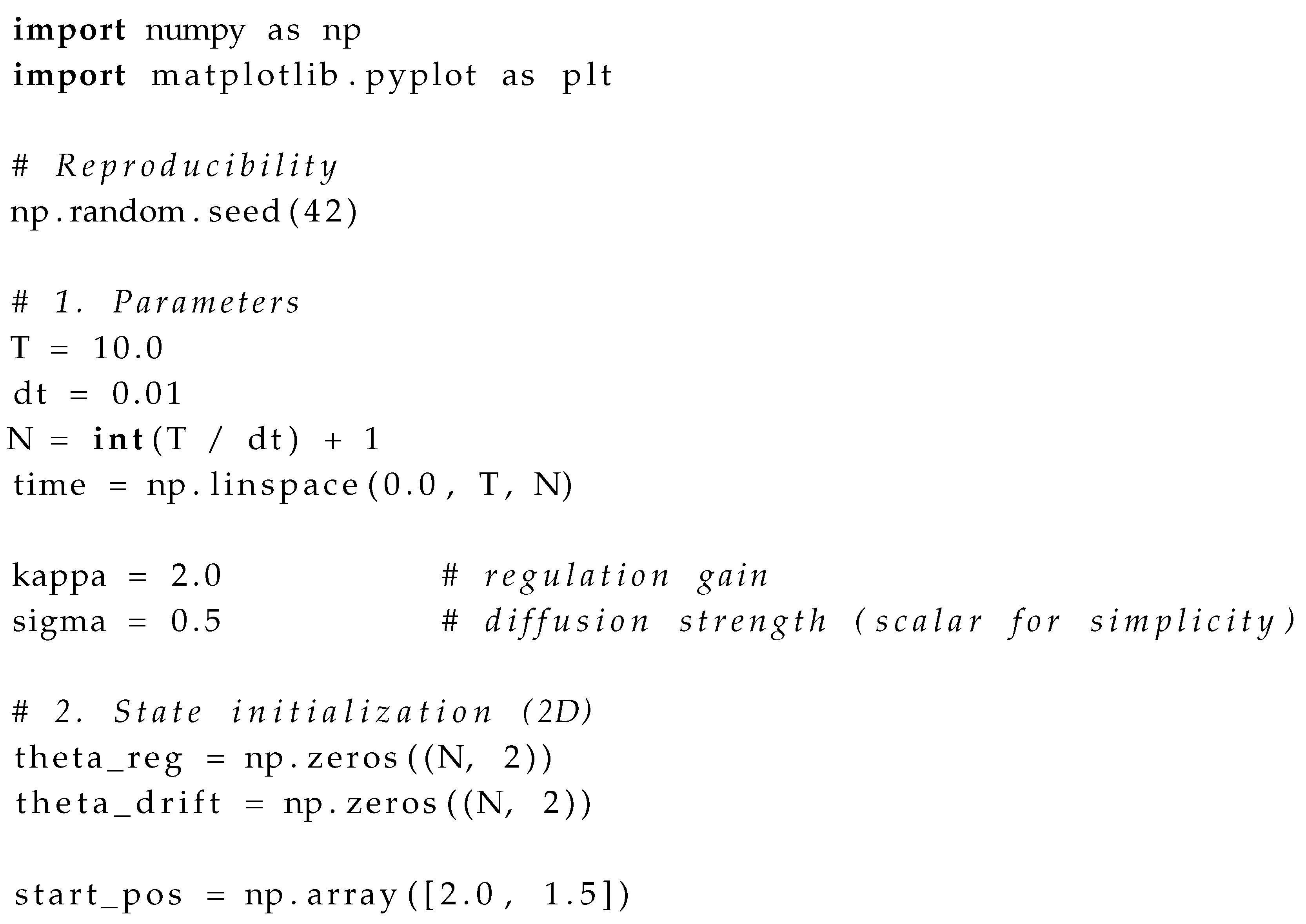
To illustrate the interplay between diffusion and feedback in the local regime, the linearized case with and is simulated:
which is the multivariate Ornstein–Uhlenbeck process. This is an illustration of local return-to-reference dynamics, not a claim that global epigenetic regulation is linear. In this simulation, the noise structure corresponds to the isotropic choice in Eq. (3).
4.1. Simulation Setup
- Dimension: for visualization.
- Initial condition: .
- Fair comparison: The regulated and unregulated trajectories use the same Wiener increments to isolate the effect of the drift term.
4.2. Results
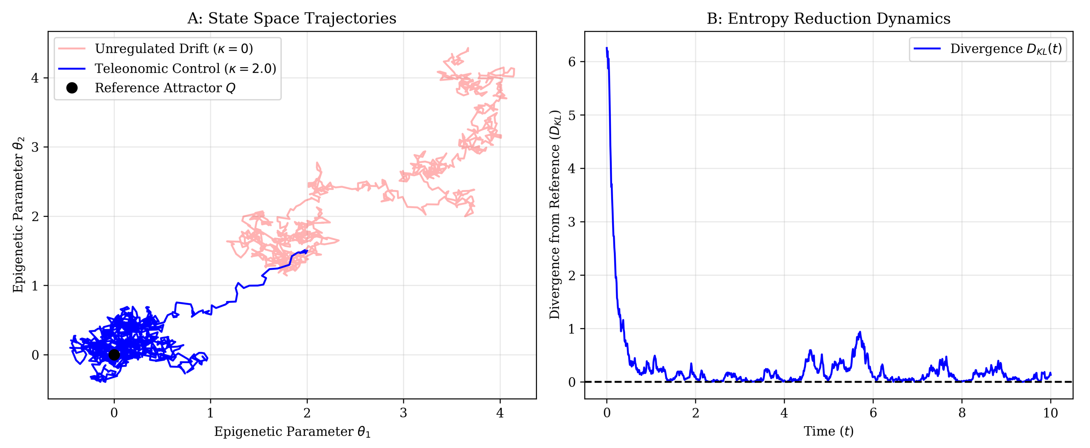
Figure 1 shows:
- 1.
- Drift vs. control: With , trajectories behave as Brownian motion with variance that grows in time.
- 2.
- Bounded fluctuations: With , trajectories are constrained to a bounded region around the reference.
- 3.
- Return-to-reference proxy: In the OU regime, a natural local proxy for distance-to-reference is , which decays in expectation toward a stationary fluctuation level under feedback.
5. Discussion
5.1. Model Limitations and Scope
The OU dynamics used in simulation are a local approximation. Far-from-equilibrium transitions and multi-attractor landscapes require nonlinear and potentially state-dependent diffusion. The present contribution is therefore best interpreted as a control-theoretic template for connecting measured signals to return-to-reference dynamics, with explicit parameters that can be estimated.
5.2. Biological Interpretation of Parameters
The regulation gain corresponds to aggregate chromatin maintenance and remodeling activity. The coupling captures how mediators project onto sensitive regulatory axes. Specific molecular substrates include ATP-dependent chromatin remodelers (e.g., SWI/SNF complex) and modifying enzymes (e.g., DNMTs, HATs); mechanistic background is reviewed in [5]. The diffusion term captures effective stochasticity from biochemical fluctuations and resource variability.
5.3. Diffusion Bridges and a Constrained-Process Analogy (Teleonomy as Present-Time Drift)
A common mathematical representation of “goal constraints” in stochastic systems is conditioning a diffusion on an endpoint event (a bridge process). Consider an Itô diffusion
Conditioning on an endpoint (e.g., ) yields a bridge whose drift can be written via Doob’s h-transform:
with proportional to a transition density toward the conditioned event [14,15]. For Brownian motion this recovers the classical Brownian bridge drift. In our setting, this provides an analogy: global viability constraints can be represented as additional present-time drift terms. In local regimes, such drifts can be approximated by linear restoring forces, motivating why a feedback form like is a natural modeling choice. This is an analogy rather than an identity: the exact correspondence depends on the specific conditioning event and the associated h.
5.4. Implications for Intervention Specificity (Projection Condition)
The model clarifies why not every input produces specific remodeling: effective steering requires that the lagged signal has a non-zero projection onto sensitive directions of the local Hessian landscape. If inputs are orthogonal to these directions, return-to-reference behavior is governed mainly by feedback and diffusion rather than by signal-induced steering.
6. Conclusions
Epigenetic Teleonomy provides a falsifiable framework: effective regulation should manifest as a measurable reduction in divergence-to-reference relative to an empirically defined baseline, while stability requires sufficient gain relative to diffusion strength. Future work should estimate , , , and from time-series epigenomic measurements.
Author Contributions
The author conceived the theoretical framework, performed the mathematical derivations, implemented the numerical simulations, and wrote the manuscript.
Funding
This research received no external funding.
Informed Consent Statement
Not applicable.
Data Availability Statement
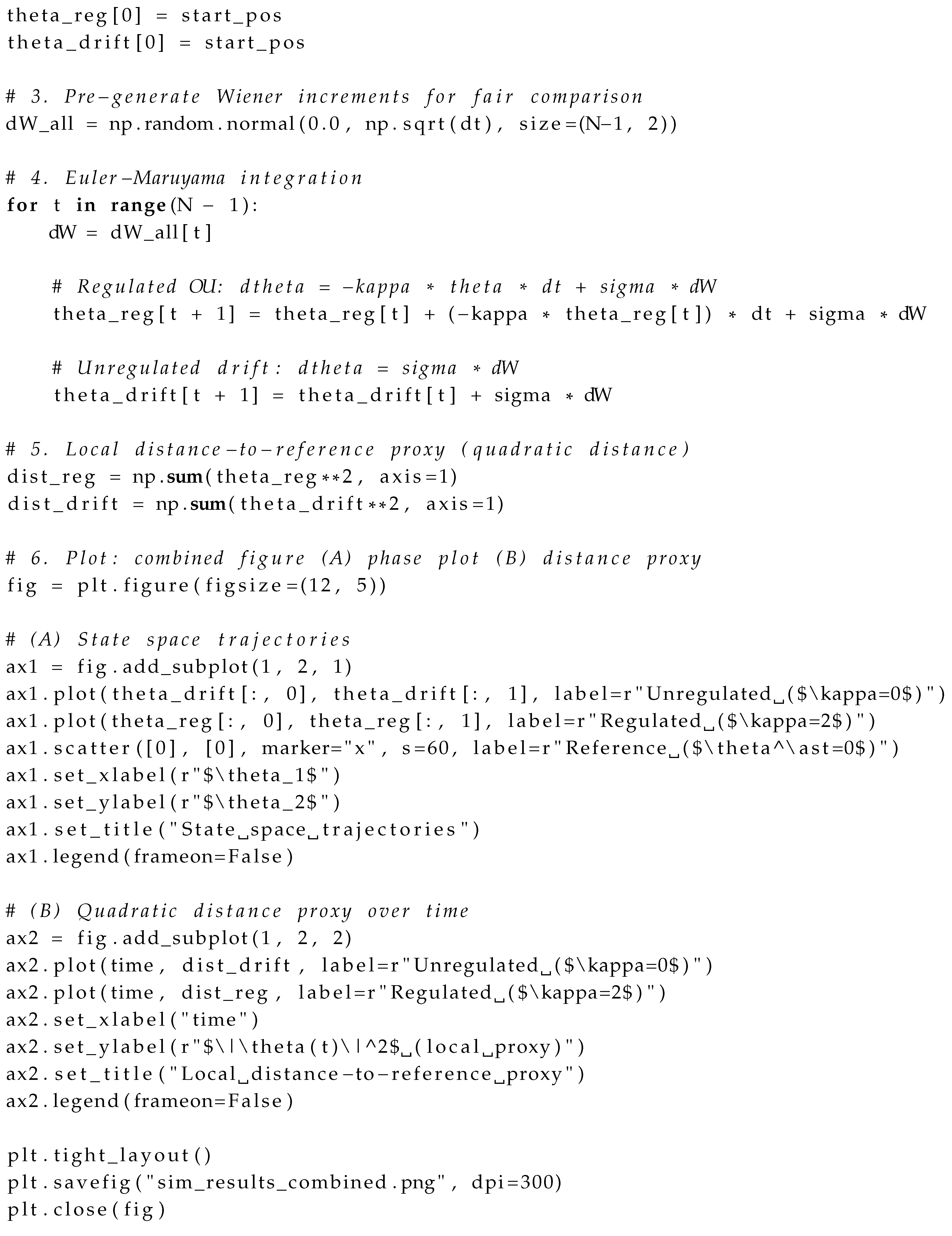
No external datasets were used. All results are reproducible from the simulation code provided in Appendix B, which generates Figure 1.
Conflicts of Interest
The author declares no conflict of interest.
Abbreviations and Notation

Table 1.
Abbreviations used in this manuscript.
| Abbreviation | Definition |
|---|---|
| SDE | Stochastic differential equation |
| OU | Ornstein–Uhlenbeck (return-to-reference) process |
| CpG | Cytosine-phosphate-Guanine dinucleotide |
| DNMT | DNA methyltransferase |
| HAT | Histone acetyltransferase |
| SWI/SNF | Switch/Sucrose Non-Fermentable (chromatin remodeling complex) |
| ATAC-seq | Assay for Transposase-Accessible Chromatin with high-throughput sequencing |
Table 2.
Notation used in this manuscript.
| Symbol | Description |
|---|---|
| High-dimensional epigenetic microstate vector | |
| Instantaneous probability distribution of the microstate | |
| Observable assay vector (projection of microstate) | |
| Observable distribution parametrized by | |
| Epigenetic state vector (order parameters) | |
| Reference regime distribution (within-subject baseline) | |
| / | Kullback–Leibler divergence (relative entropy to reference) |
| Potential defined as | |
| Regulation gain (feedback strength) | |
| Context signal vector (mediators) | |
| Actuation/coupling matrix | |
| Temporal kernel (lag/hysteresis) | |
| Noise covariance matrix | |
| Wiener process (Brownian motion) | |
| A | Local Hessian of at |
| Expectation operator |
Appendix A Stability in the Local Quadratic Regime
Appendix A.1. A.1 Local quadratic approximation
Assume is a local reference point (e.g., a mode of the reference basin) and
Then and, neglecting bounded inputs for the moment, Eq. (3) becomes
If A is positive definite in the basin, the process is mean-reverting (OU-type).
Appendix A.2. A.2 Lyapunov drift and stationary scaling
Let . By Itô’s Lemma [13],
With and :
For the linearized multivariate OU system, the stationary covariance C satisfies the continuous-time Lyapunov equation
In the isotropic special case , this reduces to (and for scalar gives ).
Appendix A.3. A.3 Bounded-input remark (input-to-state stability intuition)
If the lagged input term is bounded in norm and locally, standard linear systems intuition implies the state remains bounded in expectation around a shifted mean. This motivates treating signal transduction as steering within (or between) basins while feedback stabilizes against diffusion.
Appendix A.4. A.4 Diffusion bridges and Doob’s h-transform (formal statement)
For an Itô diffusion with , conditioning on an endpoint event can be represented by a Doob h-transform, yielding an additional drift term under suitable regularity assumptions [14,15]. This provides a principled way to interpret constraints as present-time drift terms, though the exact mapping depends on the chosen conditioning event and transition kernel.
Appendix B Appendix B: Python Code for Numerical Simulation
Listing 1: Reproducible simulation and plotting (OU illustration)
References
- Bird, A. (2007). Perceptions of epigenetics. Nature, 447, 396–398. [CrossRef]
- Jenuwein, T., & Allis, C. D. (2001). Translating the histone code. Science, 293, 1074–1080. [CrossRef]
- McEwen, B. S., & Wingfield, J. C. (2003). The concept of allostasis in biology and biomedicine. Hormones and Behavior, 43, 2–15. [CrossRef]
- Teschendorff, A. E., et al. (2016). DNA methylation outliers in normal breast tissue identify field defects that are enriched in cancer. Nature Communications, 7, 10478. [CrossRef]
- Clapier, C. R., et al. (2017). Mechanisms of action and regulation of ATP-dependent chromatin-remodelling complexes. Nature Reviews Molecular Cell Biology, 18, 407–422. [CrossRef]
- Landauer, R. (1961). Irreversibility and Heat Generation in the Computing Process. IBM Journal of Research and Development, 5, 183–191. [CrossRef]
- Shannon, C. E. (1948). A Mathematical Theory of Communication. Bell System Technical Journal, 27, 379–423. [CrossRef]
- Friston, K. (2010). The free-energy principle: a unified brain theory? Nature Reviews Neuroscience, 11, 127–138. [CrossRef]
- Levin, M. (2019). The Computational Boundary of a “Self”. Frontiers in Psychology, 10, 2688. [CrossRef]
- Waddington, C. H. (1957). The Strategy of the Genes. Allen & Unwin. (Reprint 2014 Routledge, ISBN: 9781138017313).
- Uhlenbeck, G. E., & Ornstein, L. S. (1930). On the Theory of the Brownian Motion. Physical Review, 36, 823. [CrossRef]
- Kloeden, P. E., & Platen, E. (1992). Numerical Solution of Stochastic Differential Equations. Springer. [CrossRef]
- ksendal, B. (2003). Stochastic Differential Equations: An Introduction with Applications (6th ed.). Springer. [CrossRef]
- Doob, J. L. (1957). Conditional Brownian motion and the boundary limits of harmonic functions. Bulletin de la Société Mathématique de France, 85, 431–458. [CrossRef]
- Baudoin,, F. (2002). Conditioned stochastic differential equations: Theory, examples and application to finance. Stochastic Processes and their Applications, 100(1–2), 109–145. doi:10.1016/S0304-4149(02)00109-6.
Figure 1.
Local return-to-reference dynamics in the linearized regime. (A) State space trajectories for identical noise realizations: without feedback (red, ) the path diffuses, while feedback (blue, ) yields return-to-reference dynamics. (B) Local quadratic distance-to-reference proxy in the OU approximation: the regulated regime exhibits decay (in expectation) toward a stationary fluctuation level, consistent with bounded variance scaling with diffusion strength and inverse gain in the isotropic case.
Figure 1.
Local return-to-reference dynamics in the linearized regime. (A) State space trajectories for identical noise realizations: without feedback (red, ) the path diffuses, while feedback (blue, ) yields return-to-reference dynamics. (B) Local quadratic distance-to-reference proxy in the OU approximation: the regulated regime exhibits decay (in expectation) toward a stationary fluctuation level, consistent with bounded variance scaling with diffusion strength and inverse gain in the isotropic case.
Disclaimer/Publisher’s Note: The statements, opinions and data contained in all publications are solely those of the individual author(s) and contributor(s) and not of MDPI and/or the editor(s). MDPI and/or the editor(s) disclaim responsibility for any injury to people or property resulting from any ideas, methods, instructions or products referred to in the content. |
© 2026 by the authors. Licensee MDPI, Basel, Switzerland. This article is an open access article distributed under the terms and conditions of the Creative Commons Attribution (CC BY) license (http://creativecommons.org/licenses/by/4.0/).
Copyright: This open access article is published under a Creative Commons CC BY 4.0 license, which permit the free download, distribution, and reuse, provided that the author and preprint are cited in any reuse.