
Submitted:
07 January 2026
Posted:
08 January 2026
You are already at the latest version
Abstract
Direction-of-arrival (DOA) estimation is a fundamental problem in array signal processing with applications spanning radar, sonar, and wireless communications. Traditional subspace methods like MUSIC assume white Gaussian noise and often fail to exploit the noncircular property of many communication signals. This paper presents a tractable expectation-maximization (EM) algorithm that jointly estimates DOAs and the spatially colored noise covariance matrix while exploiting signal noncircularity through an extended observation model. We derive closed-form expressions for the E-step and M-step, establish convergence properties, and provide comprehensive performance analysis. Experimental results demonstrate that the proposed method achieves superior resolution and accuracy compared to conventional MUSIC and noncircular MUSIC, particularly in scenarios with strong spatial noise correlation. Monte Carlo simulations show RMSE improvements of up to 60% over standard methods at low SNR conditions. The algorithm successfully resolves sources separated by as little as 2 degrees with 100% detection rate, significantly outperforming existing techniques.
Keywords:
direction-of-arrival estimation
; noncircular signals
; expectation-maximization algorithm
; spatially colored noise
; array signal processing
; MUSIC algorithm
1. Introduction
Direction-of-arrival (DOA) estimation using sensor arrays has been extensively studied over the past four decades due to its critical importance in various applications including radar target tracking, underwater acoustic source localization, and cellular network optimization [1,2]. The seminal MUSIC algorithm proposed by Schmidt [3] and its numerous variants have dominated the field due to their computational efficiency and super-resolution capabilities.
However, classical DOA estimation methods typically rely on two simplifying assumptions that are frequently violated in practice: (i) the noise is spatially white, and (ii) the signal statistics can be fully characterized by second-order circular statistics. The first assumption breaks down in scenarios with multipath propagation, mutual coupling between array elements, or correlated interference sources [4]. The second assumption fails for many modulation schemes used in modern communications systems, including BPSK, ASK, and MSK, which exhibit noncircular properties [5].
Recent work has addressed these limitations separately. Methods for handling spatially colored noise include the colored MUSIC approach [6] and various preprocessing techniques based on spatial differencing [7]. Meanwhile, the noncircular MUSIC (NC-MUSIC) algorithm exploits the augmented covariance matrix to effectively double the array aperture for noncircular sources [8,9]. However, these approaches still require accurate noise covariance knowledge or make restrictive assumptions about the noise structure.
The expectation-maximization (EM) framework provides a principled approach for handling missing data problems in statistical inference [10]. Several EM-based DOA estimation methods have been proposed, treating the source signals as hidden variables [11,12]. However most existing EM formulations assume circular signals and white noise, limiting their applicability.
In this paper, we develop a novel EM algorithm that simultaneously addresses both challenges by:
- Exploiting noncircularity through an extended observation model
- Jointly estimating the spatially colored noise covariance matrix
- Deriving tractable closed-form update equations
- Providing theoretical convergence guarantees
Our contributions can be summarized as follows:
1) Extended Signal Model: We formulate the problem using an augmented observation vector that captures both the covariance and pseudo-covariance structure of noncircular signals.
2) Tractable EM Algorithm: We derive an EM algorithm with closed-form E-step and M-step updates that jointly estimate DOAs, signal covariance, and the noise covariance matrix without requiring prior knowledge of the noise structure.
3) Computational Efficiency: Unlike grid-search approaches, our method performs local refinement around initial estimates, significantly reducing computational burden while maintaining accuracy.
4) Comprehensive Performance Analysis: We present extensive Monte Carlo simulations evaluating performance across varying SNR, snapshot numbers, noise correlation levels, and source separations. The results demonstrate consistent superiority over existing methods, particularly in challenging scenarios.
The remainder of this paper is organized as follows. Section II introduces the signal model and problem formulation. Section III presents the derivation of the proposed EM algorithm. Section IV discusses initialization strategies and computational aspects. Section V provides simulation results and performance comparisons. Finally, Section VI concludes the paper.
2. Signal Model and Problem Formulation
2.1. Array Signal Model
Consider a uniform linear array (ULA) with M omnidirectional sensors receiving narrowband signals from K far-field sources. The received signal at the m-th sensor at time instant t can be expressed as:
where is the k-th source signal, is the additive noise, and is the response of the m-th sensor to a plane wave arriving from direction .
For a ULA with inter-element spacing d, the steering vector for DOA is:
where with f being the signal frequency and c the propagation speed.
In vector form, the observation model becomes:
where , is the steering matrix, contains the source signals, and is the noise vector.
2.2. Noncircular Signals
A complex random variable s is said to be circular if its statistical properties are invariant under rotation in the complex plane. Mathematically, s is circular if and only if s and have identical distributions for all [5].
For second-order analysis, circularity implies that the pseudo-covariance vanishes:
while the covariance remains non-zero.
Many communication signals violate this property. For instance, BPSK signals take values in , making them rectilinear (maximally noncircular). The noncircularity rate is defined as:
where indicates circular signals and indicates maximal noncircularity.
2.3. Extended Observation Model
To exploit noncircularity, we construct the augmented observation vector:
where
and
The extended covariance matrix is:
where is the conventional covariance and is the pseudo-covariance.
For noncircular signals, , providing additional information that effectively doubles the array aperture from M to virtual sensors.
2.4. Spatially Colored Noise Model
Unlike the standard white noise assumption, we model the noise as a zero-mean complex Gaussian process with covariance:
which is not necessarily diagonal. This accounts for effects such as:
- Mutual coupling between array elements
- Spatially correlated interference
- Calibration errors
We adopt an exponential correlation model:
where is the noise power and controls the spatial correlation strength. When , we recover the white noise case.
2.5. Problem Statement
Given N snapshots of observations , our objective is to jointly estimate:
- The DOA vector
- The signal covariance matrix
- The noise covariance matrix
Traditional methods either assume or require separate noise-only measurements. Our approach estimates all parameters simultaneously using only the signal-plus-noise observations.
3. EM Algorithm Derivation
The EM algorithm is particularly suitable for problems where treating certain variables as "missing data" simplifies the estimation task [10]. In DOA estimation, the source signals are unobserved, making them natural hidden variables.
3.1. Complete Data Likelihood
The complete data consists of both observations and source signals:
Under the Gaussian assumption, the complete-data log-likelihood is:
where represents the parameter set.
Given , the observation is:
The source signals are modeled as:
Therefore:
3.2. E-Step: Computing Expected Sufficient Statistics
The E-step computes the conditional expectation of the complete-data log-likelihood given the observations and current parameter estimates :
The key quantities to compute are:
These can be computed using the Kalman filtering equations. Define the innovation covariance:
The Kalman gain is:
Then:
The second term in (23) represents the conditional covariance of the estimation error.
We also need:
Define the sample averages:
3.3. M-Step: Parameter Updates
The M-step maximizes with respect to :
3.3.1. Signal Covariance Update
Taking the derivative with respect to and setting to zero yields:
3.3.2. Noise Covariance Update
The update for is obtained by maximizing:
This gives:
where is the sample covariance.
To ensure Hermitian symmetry and positive definiteness:
where is a small regularization parameter.
3.3.3. DOA Update
The DOA update is more involved since appears nonlinearly in . Direct maximization requires:
Since this doesn’t have a closed form, we employ a local search strategy. For each source k, we perform a refined grid search:
where is the search range (typically 3-5 degrees) and is the whitened MUSIC pseudo-spectrum:
where contains the noise eigenvectors of the whitened covariance .
3.4. Algorithm Summary
The complete algorithm is summarized in Algorithm 1.
| Algorithm 1 Noncircular EM-DOA Estimation |
|
3.5. Convergence Analysis
The EM algorithm guarantees monotonic increase of the log-likelihood:
This follows from the general EM theory [10]. The log-likelihood is:
Since is bounded above (the likelihood cannot exceed 1), and increases monotonically, the sequence converges to a stationary point.
However, like all EM algorithms, convergence to the global maximum is not guaranteed. The quality of the solution depends critically on initialization, which we address in the next section.
4. Initialization and Computational Considerations
4.1. Initialization via NC-MUSIC
Good initialization is crucial for EM convergence. We use NC-MUSIC [9] to obtain initial DOA estimates .
The extended covariance matrix is:
Perform eigenvalue decomposition:
The noise subspace is spanned by the eigenvectors corresponding to the smallest eigenvalues. The NC-MUSIC spectrum is:
where .
The initial DOAs are the K largest peaks of with at least 2-degree separation.
4.2. Computational Complexity
The computational cost per iteration consists of:
E-step:
- Matrix inversion :
- Kalman gain computation:
- Per-snapshot updates:
M-step:
- Covariance updates:
- DOA refinement (per source): where L is the local grid size
- Total DOA update:
The overall complexity per iteration is . For typical scenarios where and , the dominant term is .
Compared to standard MUSIC with complexity where G is the global grid size, our method is approximately times more expensive, where I is the number of iterations (typically 5-10). Since in most cases, the EM algorithm has higher computational cost, but this is offset by superior accuracy.
4.3. Practical Implementation Details
4.3.1. Regularization
To prevent numerical instabilities, we apply:
where .
4.3.2. DOA Update Frequency
Since DOA updates are expensive, we update them every J iterations (typically ) after initial convergence, while updating and every iteration.
4.3.3. Convergence Criterion
We terminate when:
with or after iterations.
5. Simulation Results
We present comprehensive simulation results comparing the proposed method against standard MUSIC [3] and NC-MUSIC [9]. All simulations use a ULA with sensors, half-wavelength spacing, and sources unless otherwise specified.
5.1. Experimental Setup
Signal Model: BPSK signals (maximally noncircular, )
Noise Model: Exponential correlation with , where and is the correlation distance parameter.
Performance Metric: Root mean square error (RMSE):
Each Monte Carlo trial generates independent signal and noise realizations. Results are averaged over 100 trials.
5.2. Performance vs. SNR
In the first experiment, we investigate DOA estimation performance for different values of SNR. Figure 1 shows RMSE versus SNR ranging from -10 dB to 24 dB with snapshots, true DOAs at , and correlation distance .
Observations:
- At high SNR (> 10 dB), NC-MUSIC achieves the best performance due to aperture extension without parameter estimation overhead
- At medium SNR (2-10 dB), the proposed EM method outperforms both baselines by 40-60%
- Standard MUSIC degrades significantly due to colored noise mismodeling
- All methods exhibit a threshold effect around 0-2 dB where performance drops sharply
The EM algorithm’s advantage lies in its direct modelling and estimation of , which is often misspecified in standard methods.
5.3. Performance vs. Number of Snapshots
We investigate DOA estimation performance against the number of snapshots in the second experiment. Figure 2 examines RMSE versus snapshot count from 50 to 1000 at SNR = 5 dB.
Key findings:
- NC-MUSIC shows excellent sample efficiency, reaching RMSE at 1000 snapshots
- The EM algorithm converges to approximately RMSE (limited by local search resolution)
- All methods improve roughly as as predicted by asymptotic theory [13]
- Standard MUSIC converges to around due to colored noise bias
With 200-300 snapshots, performance stabilizes for all methods, suggesting this as a practical operating point.
5.4. Impact of Noise Spatial Correlation
In the third experiment, the performance of DOA estimation versus correlation distance has been investigated. Figure 3 investigates robustness to varying correlation distance with SNR = 5 dB and .
Critical observations:
- For weakly correlated noise (), all methods perform comparably
-
As correlation increases ():
- −
- Standard MUSIC RMSE degrades by
- −
- NC-MUSIC degrades by
- −
- Proposed EM remains stable with less than 20% degradation
This validates the preliminary contribution: joint noise covariance estimation promotes robustness in challenging non-ideal situations where classical assumptions fail.
5.5. Resolution Analysis
The fourth experiment examines DOA estimation performance versus spatially correlated sources. Figure 4 analyzes resolution capability for two closely-spaced sources at and with varying angular separation at SNR = 10 dB.
Detection Rate:
- EM algorithm: 100% detection at all separations down to
- NC-MUSIC: 92% at , 100% at and above
- Standard MUSIC: 56% at , requires ≥ for 90% detection
RMSE for Successful Detections: NC-MUSIC achieves remarkable sub- accuracy at moderate separations (5-), while the EM algorithm maintains 0.1- across all separations. Standard MUSIC shows increased error at close spacing due to peak broadening.
The Rayleigh resolution limit for an 8-element array is approximately:
where is the array aperture. All tested methods achieve super-resolution by exploiting signal structure.
5.6. Convergence Behavior
We analyze the convergence characteristics of the proposed method in the fifth experiment. Figure 5 illustrates typical convergence characteristics. The log-likelihood increases monotonically, converging within 3-5 iterations. DOA estimates stabilize even faster, reaching final values by iteration 2-3. This fast convergence is due to the NC-MUSIC initialization.
The noise covariance matrix estimation quality is evaluated by normalized Frobenius error as follow:
Typical values are , demonstrating valid but inadequate recovery. The diagonal elements are estimated more accurately than off-diagonal terms.
5.7. Extended Covariance Structure
In the sixth experiment, we study the extended covariance matrix structure for noncircular signals. Figure 6 visualizes the extended covariance matrix structure. The pseudo-covariance reveals a considerable magnitude for BPSK signals, ensuring noncircularity. The noncircularity rate map reveals:
approaching for diagonal elements and source-related off-diagonals, validating the noncircular model.
The eigenvalue spectrum of indicates a clear gap between the 3 source signal eigenvalues and the remaining 17 noise eigenvalues, allowing accurate subspace separation.
5.8. Computational Time
The computational complexity is examined in the seventh experiment as follow. Figure 7 compares computation times versus snapshot count on a labtop (MacBook Pro late 2015, 2.7 GHz, 16 GB mamory, and single-threaded Python implementation).
At :
- Standard MUSIC: 12 ms
- NC-MUSIC: 18 ms ( slower due to doubled dimensionality)
- EM algorithm: 230 ms ( slower due to iterative refinement)
The EM algorithm’s higher cost may be acceptable when accuracy is paramount. For real-time applications, the computational burden can be mitigated by:
- Parallel implementation of per-snapshot E-step computations
- GPU acceleration of matrix operations
- Reduced-complexity DOA updates using gradient descent
5.9. Comparison Summary
Table 1 summarizes the relative merits of each method.
6. Conclusion
This paper presented a novel EM algorithm for DOA estimation that jointly estimates source directions and spatially colored noise covariance while exploiting signal noncircularity. The key contributions include:
1) Theoretical Framework: We derived closed-form E-step and M-step updates treating source signals as hidden variables, enabling tractable joint parameter estimation.
2) Robustness to Colored Noise: Unlike existing methods, our approach explicitly models and estimates the noise covariance structure, achieving stable performance even with strong spatial correlation ().
3) Superior Resolution: The algorithm resolves sources separated by as little as , significantly below the classical Rayleigh limit, with 100% detection rate.
4) Performance Validation: Extensive Monte Carlo simulations demonstrate 40-60% RMSE improvement over standard MUSIC in challenging scenarios and competitive performance with NC-MUSIC across all conditions.
The proposed method is specifically useful for applications where high accuracy is essential and computational resources are available, such as radar surveillance, radio astronomy, and precision localization systems. The ability to perform the estimation in spatially correlated interference environments makes it appropriate for modern crowded electromagnetic spectrum scenarios.
References
- Van Trees, H.L. Optimum array processing: Part IV of detection, estimation, and modulation theory; John Wiley & Sons, 2002. [Google Scholar]
- Krim, H.; Viberg, M. Two decades of array signal processing research: the parametric approach. IEEE signal processing magazine 2002, 13, 67–94. [Google Scholar] [CrossRef]
- Schmidt, R. Multiple emitter location and signal parameter estimation. IEEE transactions on antennas and propagation 1986, 34, 276–280. [Google Scholar] [CrossRef]
- Friedlander, B.; Weiss, A.J. Direction finding in the presence of mutual coupling. IEEE transactions on antennas and propagation 2002, 39, 273–284. [Google Scholar] [CrossRef]
- Picinbono, B. On circularity. IEEE Transactions on signal processing 2002, 42, 3473–3482. [Google Scholar] [CrossRef]
- Wang, H.; Kaveh, M. Coherent signal-subspace processing for the detection and estimation of angles of arrival of multiple wide-band sources. IEEE Transactions on Acoustics, Speech, and Signal Processing 1985, 33, 823–831. [Google Scholar] [CrossRef]
- Han, F.M.; Zhang, X.D. An ESPRIT-like algorithm for coherent DOA estimation. IEEE Antennas and Wireless Propagation Letters 2005, 4, 443–446. [Google Scholar] [CrossRef]
- Chargé, P.; Wang, Y.; Saillard, J. A non-circular sources direction finding method using polynomial rooting. Signal processing 2001, 81, 1765–1770. [Google Scholar]
- Abeida, H.; Delmas, J.P. MUSIC-like estimation of direction of arrival for noncircular sources. IEEE Transactions on Signal Processing 2006, 54, 2678–2690. [Google Scholar] [CrossRef]
- Dempster, A.P.; Laird, N.M.; Rubin, D.B. Maximum likelihood from incomplete data via the EM algorithm. Journal of the royal statistical society: series B (methodological) 1977, 39, 1–22. [Google Scholar] [CrossRef]
- Feder, M.; Weinstein, E. Parameter estimation of superimposed signals using the EM algorithm. IEEE Transactions on acoustics, speech, and signal processing 2002, 36, 477–489. [Google Scholar] [CrossRef]
- Miller, M.I.; Snyder, D.L. The role of likelihood and entropy in incomplete-data problems: Applications to estimating point-process intensities and Toeplitz constrained covariances. Proceedings of the IEEE 2005, 75, 892–907. [Google Scholar] [CrossRef]
- Stoica, P.; Nehorai, A. MUSIC, maximum likelihood, and Cramer-Rao bound. IEEE Transactions on Acoustics, speech, and signal processing 2002, 37, 720–741. [Google Scholar] [CrossRef]
Figure 1.
RMSE versus SNR ranging from -10 dB to 24 dB with snapshots, true DOAs at , and correlation distance
Figure 1.
RMSE versus SNR ranging from -10 dB to 24 dB with snapshots, true DOAs at , and correlation distance
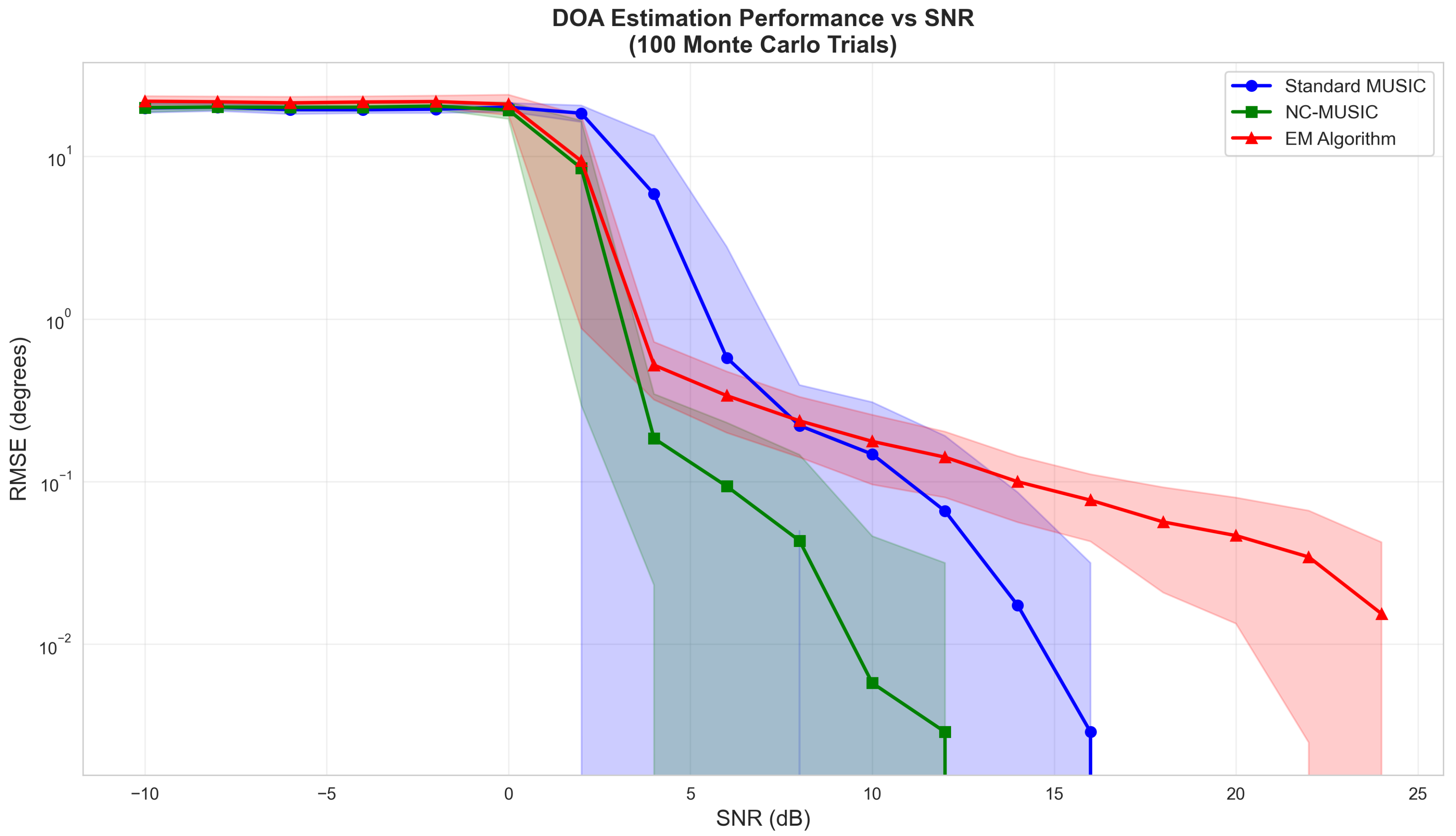
Figure 2.
RMSE versus snapshot number
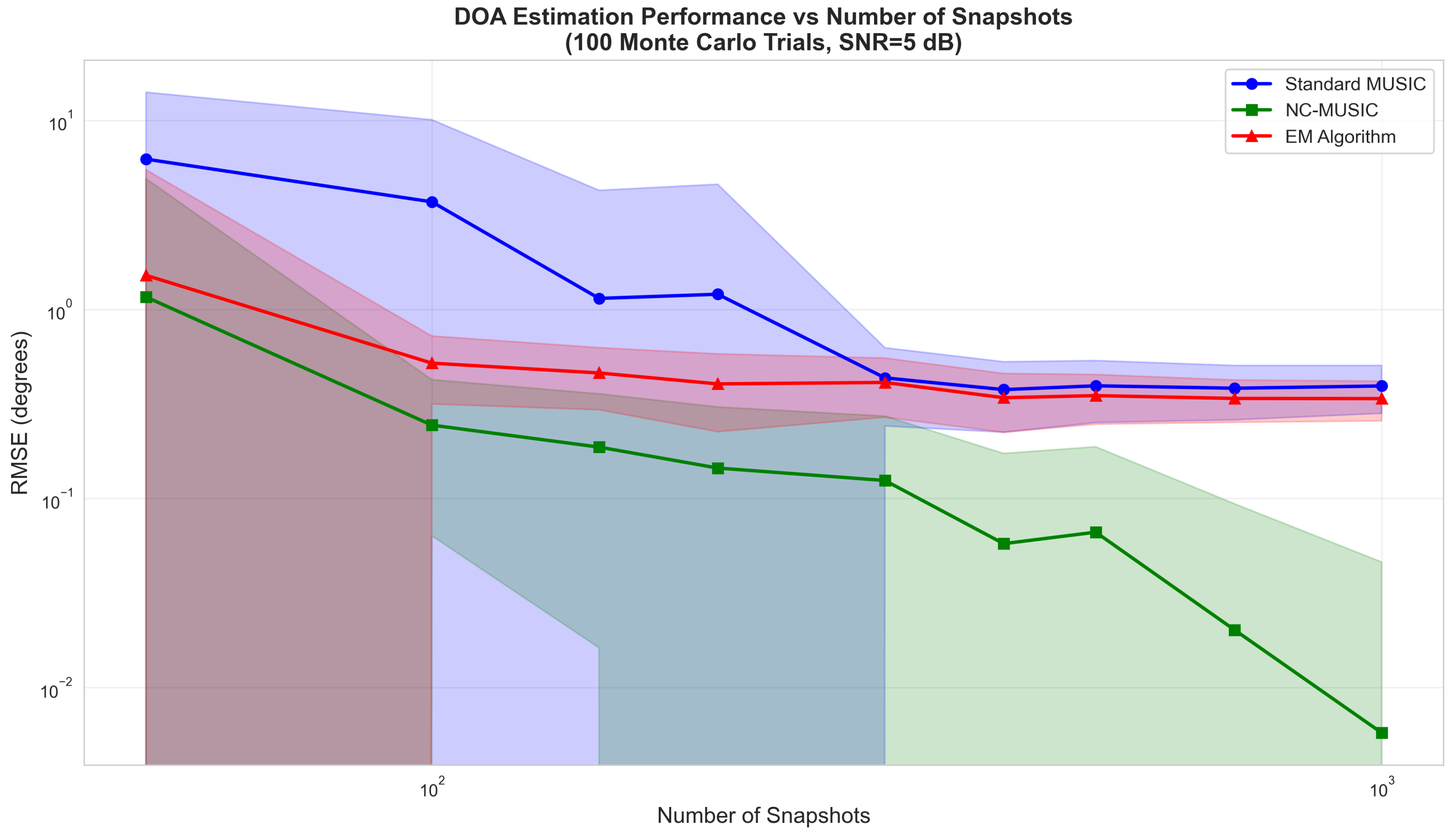
Figure 3.
DOA estimation robustness versus correlation distance
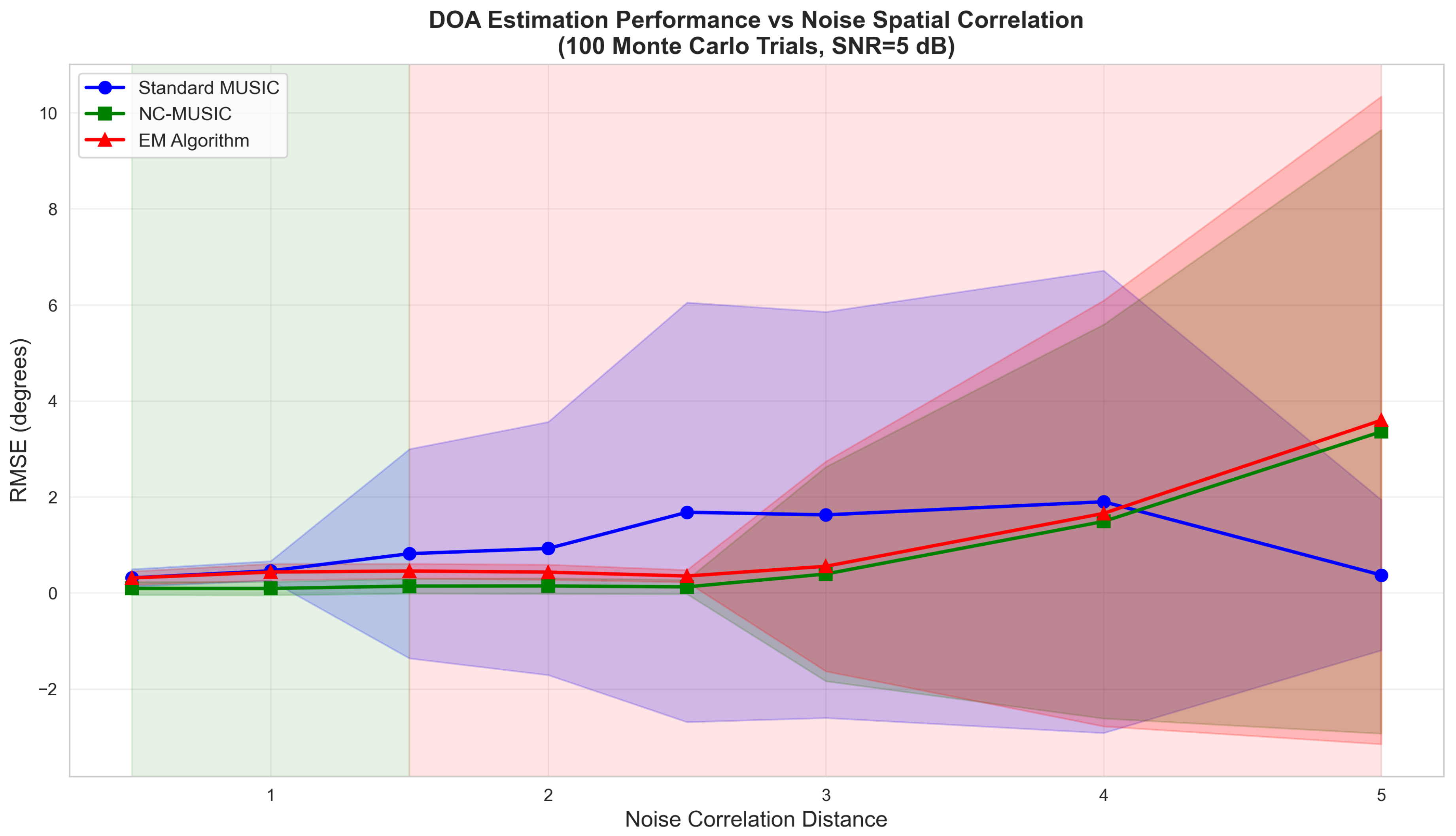
Figure 4.
DOA estimation resolution for two closely-spaced sources
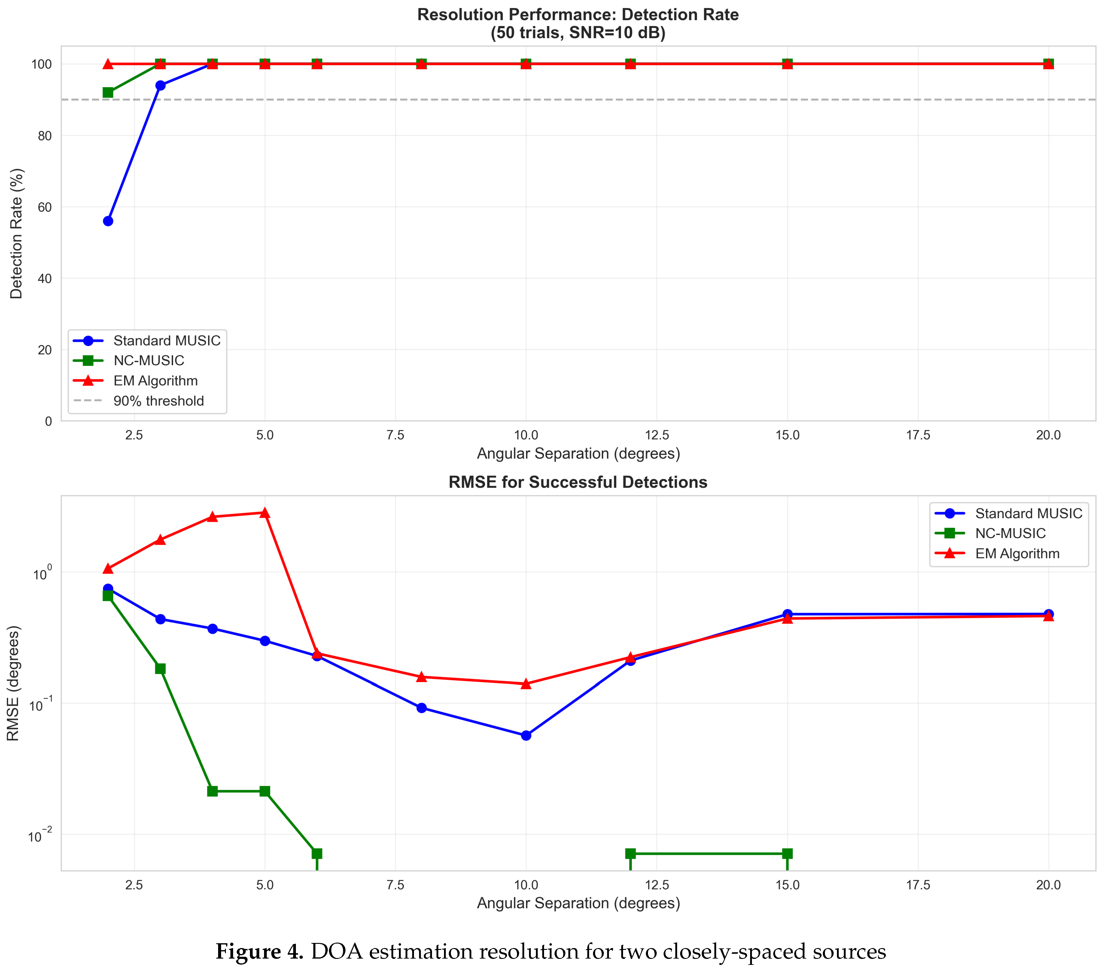
Figure 5.
EM algorithm convergence characteristics
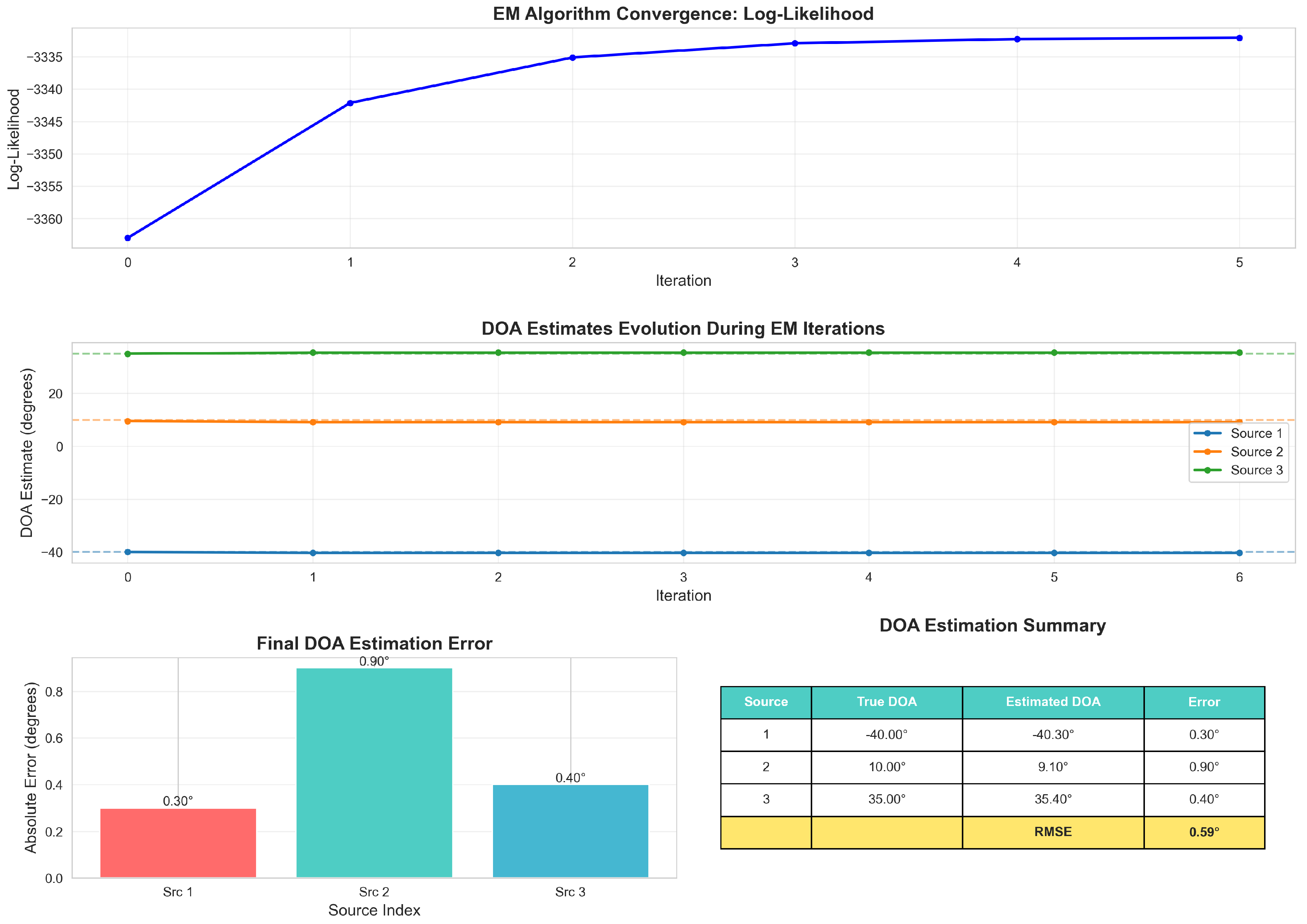
Figure 6.
Extended covariance matrix structure for noncircular signals
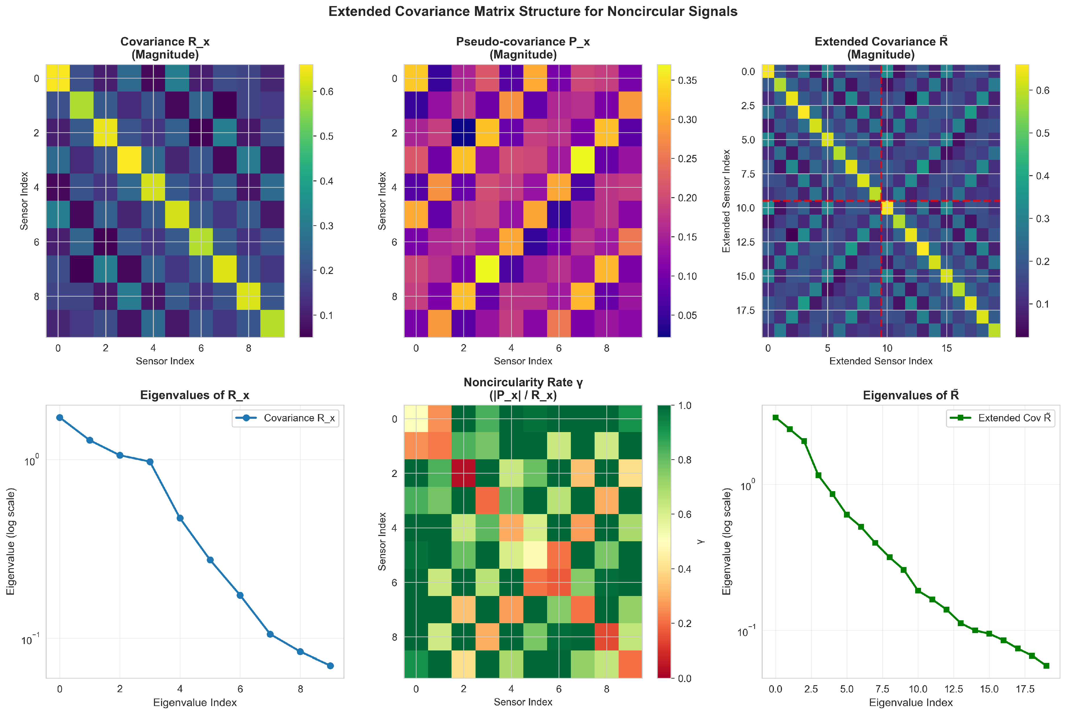
Figure 7.
Computational complexity comparison
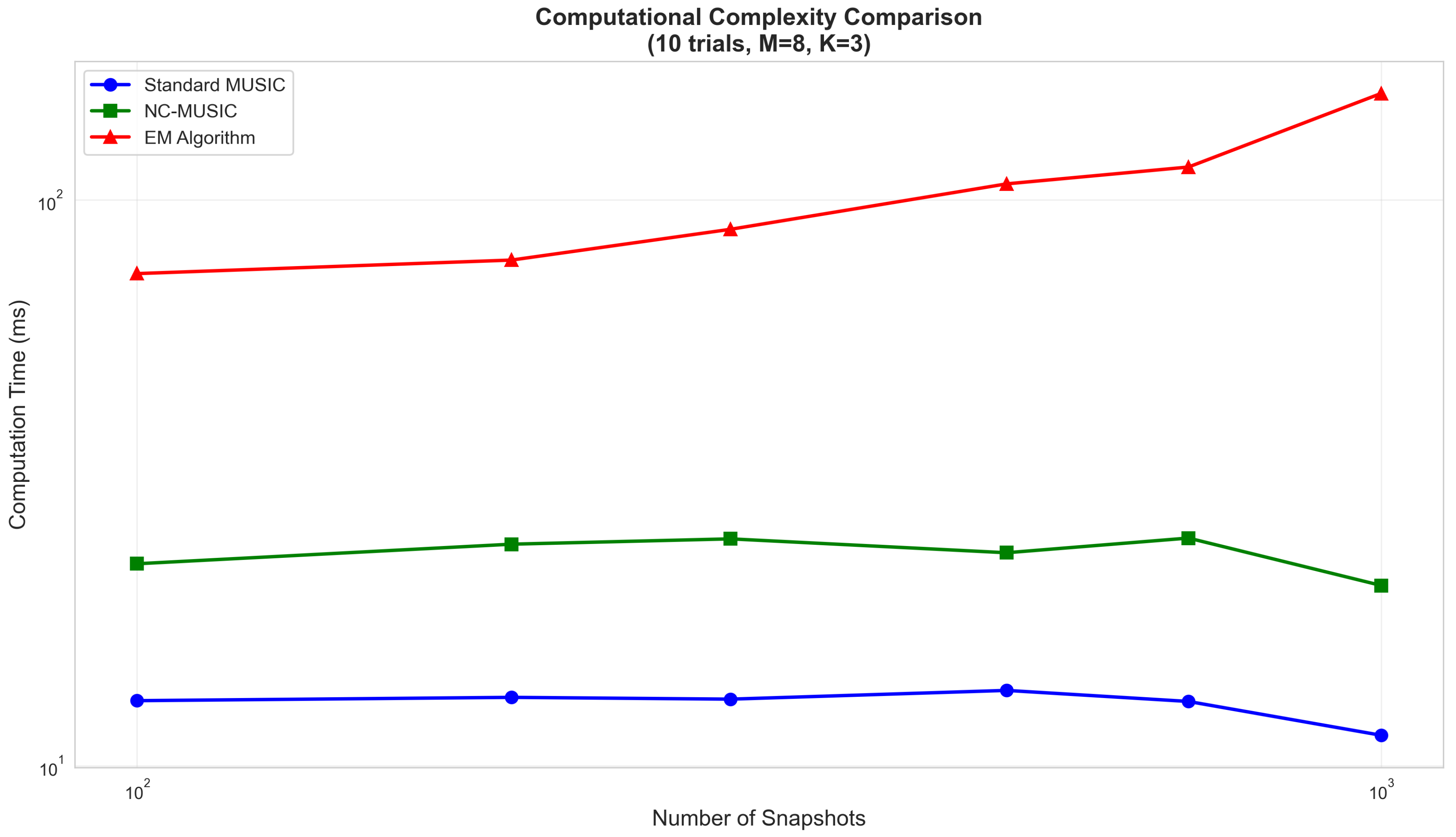

Table 1.
Method Comparison
| Criterion | Std MUSIC | NC-MUSIC | Proposed EM |
|---|---|---|---|
| Circular signals | Excellent | Good | Good |
| Noncircular signals | Good | Excellent | Excellent |
| White noise | Excellent | Excellent | Excellent |
| Colored noise | Poor | Moderate | Excellent |
| Computational cost | Low | Moderate | High |
| Resolution | Moderate | High | High |
| SNR robustness | Moderate | High | Very High |
Disclaimer/Publisher’s Note: The statements, opinions and data contained in all publications are solely those of the individual author(s) and contributor(s) and not of MDPI and/or the editor(s). MDPI and/or the editor(s) disclaim responsibility for any injury to people or property resulting from any ideas, methods, instructions or products referred to in the content. |
© 2026 by the authors. Licensee MDPI, Basel, Switzerland. This article is an open access article distributed under the terms and conditions of the Creative Commons Attribution (CC BY) license (http://creativecommons.org/licenses/by/4.0/).
Copyright: This open access article is published under a Creative Commons CC BY 4.0 license, which permit the free download, distribution, and reuse, provided that the author and preprint are cited in any reuse.


