
Submitted:
06 January 2026
Posted:
08 January 2026
You are already at the latest version
Abstract
This paper presents modified Lagrange-Jacobi functions derived from the sine, exponential, and hyperbolic tangent coordinate transformations. The resulting Lagrange-Jacobi functions and their respective matrix elements for observables can be reduced to their respective Lagrange-Legendre, Lagrange-Chebyshev, and Lagrange-Gegenbauer functions. Furthermore, this paper postulates that the Lagrange-mesh functions form approximate
complete set of basis, a property implied by their approximate orthogonality.
Keywords:
coordinate transformation
; lagrange-mesh method
; lagrange-jacobi functions
; exponential mesh
; hyperbolic mesh
; trigonometric mesh
1. Introduction
The construction of accurate numerical solutions to quantum mechanical equations remain an important component in theoretical physics and chemistry. This is because the equations, like the Schrödinger equation and the few-body integrodifferential equations, can be solved exactly only for very few potential models. Such numerical solutions are used to extract many properties of quantum systems. Among the many numerical methods that researchers often rely on to generate accurate numerical solutions to quantum mechanical equations efficiently, even with “not so accurate” matrix elements [1,2], is the Lagrange-mesh method [3,4,5,6]. This method has the combined advantageous features of the finite difference method, the collocation method, and the variational method. It is for this reason that the Lagrange-mesh method tends to is more efficient than the three listed methods separately. Moreover, the Lagrange-mesh method still has room for further development.
Lagrange meshes are generally based on the zeros of orthogonal polynomials and trigonometric basis. The more popular meshes are those that are based on the zeros of classical orthogonal polynomials, such as the Laguerre mesh defined in the interval , the Hermite mesh defined in the interval , and the Jacobi mesh defined in the interval . All these meshes can be scaled, translated, and/or transformed to treat a desired non-standard domain. Some coordinate transformations lead to modified meshes that have interesting properties requiring special discussion [3,7,8,9]. This paper presents three modified Lagrange-Jacobi meshes derived from the sine, exponential, and hyperbolic tangent coordinate transformations. These transformations lead to Lagrange-mesh functions that have features desirable for describing assymptotic forms of trial wave functions for many quantum mechanical problems [10,11]. Applying coordinate transformations to quantum mechanical equations naturally transforms the equations, leading to transformed problems. This paper demonstrates ow the indicated coordinate transformations of the Jacobi mesh can be used to construct numerical solutions to quantum mechanical problems defined on finite and infinite domains.
The sine mesh is defined in the interval and is symmetrical about zero. This mesh is the same as, but shifted relative to, the cosine mesh presented in [8]. The exponential mesh is defined in the interval , like the Laguerre mesh, while the hyperbolic mesh is defined in the interval , like the Hermite mesh. These meshes lead to the shifted trigonometric Lagrange-Jacobi functions, the exponential Lagrange-Jacobi functions, and the hyperbolic Lagrange-Jacobi functions that are discussed here for the first time. The shifted trigonometric Lagrange-Jacobi functions are similar to the trigonometric Lagrange-Jacobi functions dicussed in [8]. The three sets of functions and their respective matrix elements for derivative operators can be specialised to their respective Lagrange-Legendre, Lagrange-Chebyshev, and Lagrange-Gegenbauer functions. The results of this work have application in applied matematics, computational physics and chemistry.
This paper is organised as follows. Section 2 recalls properties of the Lagrange-mesh method focusing on the regularised Lagrange-Jacobi functions. The art of modifying the Lagrange-mesh functions is also briefly discussed. Section 3 presents trigonometric Lagrange-Jacobi functions derived from the sine transformation. Special cases of these functions are discussed. Section 4 and Section 5, respectively, present the exponential Lagrange-Jacobi functions and the hyperbolic Lagrange-Jacobi functions. Matrix elements for the first order and second order derivative operators with the functions are also discussed. Illustrative applications of the three sets of functions are presented in Section 6 while conclusions are presented in Section 7.
2. Lagrange-Jacobi Functions
A set of Lagrange-Jacobi functions , where , are constructed on the Jacobi mesh. The Jacobi mesh is defined by the N roots of a classical Jacobi polynomial of order N characterised by parameters and the weight function . Regularised Lagrange-Jacobi functions are defined as
where , is the normalisation constant for the Jacobi polynomial, and a regularising function with regularising parameters . The functions 1 are infinitely differentiable and obey the Lagrange properties
where with being quadrature weights, for , and is a scalar function [3]. Property 5 follows from the assumption that the functions form a complete set of basis. The assumption is derived from property 2. Note that properties 3 and 4 are special cases of property 5 [3].
Modified Lagrange-Jacobi functions are constructed from Eq. 1 by introducing some coordinate transformation that defines a new coordinate x with a known range that may be different from that of u. For example, the cosine transformation leads to the trigonometric Lagrange-Jacobi functions [8]. In general, the modified Lagrange-Jacobi functions have the form
where . If is negative, then the absolute value is introduced to keep the modified functions real [8]. The transformation leads to the transformed quadrature and modified weight function, see Ref. [3] for details. The resulting modified Lagrange-Jacobi functions satisfy the Lagrange properties.
It is useful to determine matrix elements for the first- and second-order derivative operators since they are used to calculate the kinetic energy of quantum mechanical systems. Thus, matrix elements for the and operators constructed with the modified functions 6 are calculated from
and
respectively, where and are the boundaries of the x domain. The mathematical structure of the transformed derivative operators and in terms of u depends on the form of the transformation considered. The integrals in 8 and 9 can be readily evaluated using properties of the Lagrange-Jacobi functions [3,7].
3. Shifted Trigonometric Lagrange-Jacobi Functions
Ref. [8] discusses trigonometric Lagrange-Jacobi functions derived from the cosine transformation. The structure of this section follows that of the reference for ease of comparison. The sine coordinate transformation has the form
where . The coordinate transformation generates the modified quadrature roots and the modified quadrature weights [3]. The modified regularised Lagrange-Jacobi functions are here called shifted trigonometric Lagrange-Jacobi functions and have the form
where , with as the weight function. These functions satisfy the Lagrange properties. It is interesting to note that the functions 11 can be obtained from Eq. (7) of Ref. [8] through the translation followed by the requirement that the interval be translated to , a shifted interval.
The evaluation of the matrix elements for the operator with the regularised shifted trigonometric Lagrange-Jacobi functions leads to
following Ref. [?]. Using the Lagrange properties, the Gauss approximation of the integral has the form
where [9], , and . As can be seen, these matrix element are similar to those presented in [8] but with substituted for and vice versa, and the interval shifted to . The Gauss approximation of the matrix elements for the operator is readily evaluated as
where , , and . Again, the elements are similar to those presented in [8] but with and interchanged, while the interval is shifted to .
On one hand, trigonometric Lagrange-Jacobi functions [8] are polynomials of where . On the other hand, trigonometric Lagrange-Jacobi functions 11 are polynomials of in the interval . The two sets of trigonometric Lagrange-Jacobi functions and their respective matrix elements for the first and second derivatives are congruous but with the sine and cosine functions interchanged and their respective intervals of definition shifted relative to each other. The shifted trigonometric Lagrange-Jacobi functions are defined on an interval that is symmetric about the origin, , a property shared by the Lagrange-Fourier and the Lagrange-sinc functions. In addition, all these three types of Lagrange-mesh functions are defined as functions of .
As indicated above, the results of this section can be derived from the results of [8] by introducing the translation and requiring that the interval be replaced with . The reverse argument is also true about deducing the results of Ref. [8] from the results of this section. The argument above suggests that the fact that some trigonometric Lagrange-mesh functions are polynomials of [12] is most likely a consequence of the definition interval . If the interval is chosen to define the basis functions, then the resulting trigonometric Lagrange-mesh functions are polynomials of , instead. The shifted trigonometric Lagrange-Legendre functions and the shifted trigonometric Lagrange-Chebyshev functions are discussed below.
3.1. Shifted Trigonometric Lagrange-Legendre Functions
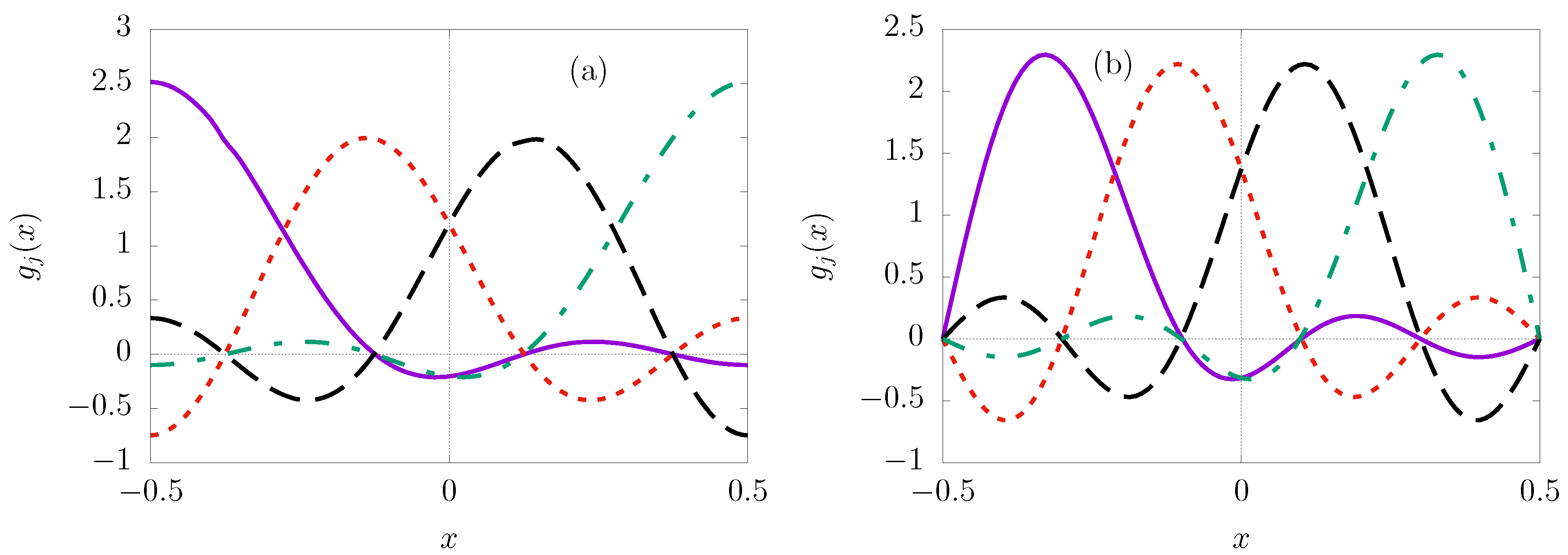
When and are both set to zero () and , Eq. 11 reduces to the shifted trigonometric Lagrange-Legendre functions
These functions are plotted in Figure 1(a) for and they are seen to vanish at the boundaries of the interval, that is, . Using the same values for , , a, and b in Eq. 13 and 14 generates, respectively, matrix elements
and
for the first and second derivatives of these functions. The elements form a symmetric matrix.
The functions 15 can be regularised so that the resulting regularised functions do not vanish at either one or both of the boundaries. For example, regularising the functions by setting leads to regularised functions that do not vanish at both boundaries. The so regularised functions have first derivatives that vanish at the boundaries, that is, . The regularised functions are plotted in Figure 1(b) for . The matrix elements and with the regularised functions are generated from Eq. 13 and Eq. 14, respectively, with the same values of the parameters , , a, and b. The resulting matrix elements form a centrosymmetric matrix that has eigenvalues where .
3.2. Shifted Trigonometric Lagrange-Chebyshev Functions
When and are both set to () and , Eq. 11 reduces to the shifted trigonometric Lagrange-Cebyshev functions
which are plotted in Figure 2(a) for . The functions are seen to be non-zero at the boundary while their first derivative vanish at the same end-points, that is, . These functions generate matrix elements that are identical to those given by Eq. 16. Their matrix elements have the form
The symmetric matrix formed by the elements has eigenvalues where .
Equation 11 generates the shifted trigonometric Lagrange-Chebyshev functions of the second kind
when and are both set to (). The functions vanish at the end-points, , as seen in Figure 2(b) for which shows a plot of these functions. Their matrix element are identical to those given by 16. Their matrix elements are given by
that form a symmetric matrix with eigenvalues where .
Figure 2.
Plots of the shifted trigonometric Lagrange-Chebyshev functions for and . (a) Functions of the first kind. (b) Functions of the second kind.
Figure 2.
Plots of the shifted trigonometric Lagrange-Chebyshev functions for and . (a) Functions of the first kind. (b) Functions of the second kind.
Equation 11 reduces to the shifted trigonometric Lagrange-Chebyshev functions of the third and fourth kind when and are set to and , respectively. The shifted trigonometric Lagrange-Chebyshev functions of the third kind display the boundary behaviour while the shifted trigonometric Lagrange-Chebyshev functions of the fourth kind display the boundary behaviour . Both kinds of functions generate matrix element that are identical to Eq. 16. In addition, both kinds of functions generate identical matrix elements
that form a symmetric matrix that has eigenvalues for .
4. Exponential Lagrange-Jacobi Functions
The exponential coordinates transformation is here defined by
and . Applying this transformation to 6 leads to the regularised exponential Lagrange-Jacobi functions
where . These functions satisfy the Lagrange conditions. When the regularising parameters are set to in 24, one obtains the exponential Lagrange-Jacobi functions. When the Jacobi polynomial parameters are set to , with , one obtains the regularised exponential Lagrange-Legendre functions. The regularised exponential Lagrange-Gegenbauer functions and the regularised exponential Lagrange-Chebyshev functions are obtained by setting and , respectively.
Figure 3(a) shows a plot of the exponential Lagrange-Legendre functions for . The functions are seen to be non-zero at the origin but approach zero as . Recall that the functions can be regularised to vanish at . The behaviour of these functions is similar to that of the Lagrange-Laguerre functions [3]. A scaling factor h can be used to shift the grid points along the x-axis for the purpose of optimising the accuracy of the results. For this purpose, the functions are modified to . Figure 3(b) displays a comparison of the exponential Lagrange-Legendre functions and the scaled exponential Lagrange-Legendre functions for and . This figure reveals the effect of have on the distribution of the grid points.
Figure 4(a) and Figure 4(b) show plots of the scaled exponential Lagrange-Chebyshev functions of the first and second kind, respectively. The functions are scaled by simply to show their behaviour at small values of x. As can be seen in the figures, the exponential Lagrange-Chebyshev functions of the first kind are non-zero at while the functions of the second kind vanish at the same point. The exponential Lagrange-Chebyshev functions of the first kind have a form similar to that of the exponential Lagrange-Legendre functions discussed above. In addition, the exponential Lagrange-Chebyshev functions of the second kind display a form similar to that of the exponential Lagrange-Chebyshev functions regularised to vanish at . Furthermore, both kinds of functions approach zero as x increases.
The construction of the matrix elements for the first-order and second-order differential operators in x requires the transformation of these operators. The transformed operators have the form
with the associated integration measure . Matrix elements of the first-order differential operator constructed with the functions 24 are calculated from
This integral is evaluated with the help of the Lagrange properties as well as properties of the Lagrange-Jacobi functions discussed in [3]. The results of the evaluation are
where . Note that use was made of the Lagrange property 5 to evaluate the integral of the first term in the square brackets in 26.
Matrix elements for the second-order differential operator calculated with the functions 24 are given by
This integral is evaluated in two steps. The first step is to evaluate the integral for the first two terms in the square brackets, independent of the factor . This leads to
where , , and . Here, use was made of the general matrix elements given in Eq. (29) of Ref. [13] by setting and . The second step is to then use the Lagrange property 5 with Eq. 28 to obtain
where . Matrix elements and for the special cases of the regularised exponential Lagrange-Jacobi functions are obtained from 27 and 31, respectively, by setting a, b, , and to their desired values.
5. Hyperbolic Lagrange-Jacobi Functions
The hyperbolic tangent coordinate transformation is defined by
with . When this transformation is applied to 6, one obtains the regularised hyperbolic Lagrange-Jacobi functions
where . These functions satisfy the Lagrange conditions. The regularised hyperbolic Lagrange-Legendre functions are obtained from Eq. 33 by setting . The regularised hyperbolic Lagrange-Chebyshev functions are obtained by setting .
Figure 5 shows plots of some of the special cases, indicated above, of the hyperbolic Lagrange-Jacobi functions 33 for . Specifically, Figure 5(a) displays the hyperbolic Lagrange-Chebyshev functions of the first kind, Figure 5(b) shows the hyperbolic Lagrange-Chebyshev functions of the second kind, and Figure 5(c) shows the hyperbolic Lagrange-Legendre functions. The plots of the three sets of functions display a form similar to that of the Lagrange-Hermite functions [3]. All the functions approach zero as the magnitude of x is increased. To assess the extent of the similarity of the functions, the functions from Figure 5(a), Figure 5(b), and Figure 5(c) are compared in Figure 5(d). As can be seen from the figure, the form of the three functions does not differ significantly.
To construct matrix elements for the first-order and second-order differential operators with the hyperbolic functions, the operator transformations
are required, with the integration measures . Using these relations, the matrix elements of the first-order differential operator constructed with the functions 33 have the form
where . Again, use was made of the Lagrange property 5 to evaluate the integral of the first term in the square brackets in 35.
Matrix elements of the second-order differential operator constructed using the functions 33 have the form
which are evaluated like in the previous subsection. Evaluating the matrix elements of the first two terms in the square brackets, i.e. without considering the factor outside the brackets, leads to
where , , and . In this case the general matrix elements in Eq. (29) of Ref. [13] are modified by setting and to obtain the elements 44. When and , the matrix formed by the elements is verified by the eigenvalues where . The elements in 37 are then evaluated as
by using the Lagrange property 5 to obtain the first term. Matrix elements and for the special cases of the regularised hyperbolic Lagrange-Jacobi functions are obtained from 36 and 40, respectively, by choosing appropriately.
6. Illustrative Applications
The one-dimensional Schrödinger equation for some potential ,
is solved numerically, where and E are the eigenfunctions and eigenvalues, respectively. Of interest are bound-state solutions of this equation which satisfy boundary conditions . The trial wave function is approximated by the expansion
where are variational parameters. This approximation generates the matrix eigenvalue problem
from Eq. 41, where the elements do not depend on h. The system of equations 43 were solved with basis sizes using different Lagrange-Jacobi functions. The relative errors of the numerical eigenvalues were calculated, where and denote numerical and analytical eigenvalues, respectively.
6.1. Shifted Trigonometric Lagrange-Jacobi Functions
An instructive example application of these functions is the one-dimensional harmonic oscillator is defined in the . This problem was solved numerical by, first, mapping the interval onto the interval where h was set to fm. The magnitude of h tends to affect the accuracy of the highly excited states in the system. The Schrödinger equation for this potential () admits exact solutions with eigenvalues where , which allow comparison with the numerical results. Then, the numerical wave functions were approximated with the shifted trigonometric Lagrange-Legendre functions () and Lagrange-Chebyshev functions ( and ). The shifted trigonometric Lagrange-Chebyshev functions of the first kind were regularised with so that the resulting functions vanish at the boundaries. For this problem, te matrix elements were calculated from
to test the validity of the matrix elements. Table 1 presents results for the relative errors of the states .
In the table, the results for the shifted trigonometric Lagrange-Legendre functions are presented in the top panel while the results for the regularised shifted trigonometric Lagrange-Chebyshev of the first kind are presented in the middle panel. The bottom panel shows results for the shifted trigonometric Lagrange-Chebyshev of the second kind. In all the three cases the results were generated using 44 for the kinetic energy matrix. As can be seen in the table, in all the three cases, the accuracy of the numerical eigenvalues improves as the basis size N is increased. The eigenvalues for lower states, and , are already obtained with machine accuracy at . The performance of the three sets of functions is almost similar. The relative errors of the eigenvalues of the excited states and are of the orders of and , respectively. The accuracy of the numerical eigenvalues for excited states is known to be dependent on the choice of the range h [14]. The results in Table 1 also verify the validity of the matrix elements in 13.
6.2. Exponential Lagrange-Jacobi Functions
The exponentially modified Lagrange-Jacobi mesh is defined in the infinite interval like the Laguerre mesh. Whereas the Laguerre mesh is spread accross the interval, the exponentially modified Lagrange-Jacobi mesh is clustered near the origin. As a result, this mesh will often need to be scaled out with to spead the mesh to the outer regions of the interval. An example application of this mesh is one of the widely used molecular potential models, the Morse potential [15]
where , a, and D are parameters related to properties of molecules. This potential has a repulsive core and a short range. The eigenvalues of the Morse potential are accurately approximated by
where . Equations 43 were solved for the Morse potential with parameters values , , , and , which were also adopted in [8] for a similar exercise. This problem was solved as indicated above with . Note that h may be optimised for more accurate results. The results for the lowest four odd eigenvalues are presented in Table 2.
The results show that the calculated lowest eigenvalues show a gradual increase in accuracy as the basis size is increased. The three sets of functions generate eigenvalues to the similar accuracy for up to . For , the regularised exponential Lagrange-Legendre and the exponential Lagrange-Chebyshev functions of the second kind generate results of similar accuracy that converge relatively faster, approximately three to six orders of magnitude, than the results of the regularised exponential Lagrange-Chebyshev functions of the first kind. Therefore, these results confirm the validity of the matrix elements in 31 and, by extention, the Lagrange property 5.
6.3. Hyperbolic Lagrange-Jacobi Functions
As indicated earlier, the hyperbolic Lagrange-Jacobi functions have a similar form as the eigen functions of the one-dimentional harmonic oscilator which are accurately represented by te Lagrange-Hermite functions. It will, therefore, be interesting to learn how accurate these functions reproduce the eigen values of the oscillator. The one-dimensional harmonic oscillator is defined in the . The Schrödinger equation for this problem has analytical solutions with eigenvalues where . It is important to note that the Hermite mesh, which supports analytical solutions to the harmonic oscillator, is well distrubuted accross the infinite interval. However, the hyperbolic tangent Lagrange-Jacobi mesh is clustered around the origin. Hence, the hyperbolic Lagrange-Jacobi functions require scaling to spread the mesh further into the outer regions of the interval.
Numerical solutions for the harmonic oscillator were constructed with the functions 33 for in the interval considering the special cases , , and . These cases correspond to the hyperbolic Lagrange-Legendre functions, the hyperbolic Lagrange-Chebyshev functions of the first kind, and the hyperbolic Lagrange-Chebyshev functions of the second kind, respectively. The effect of the basis size N on the accuracy of the calculated eigenvalues was tested by solving the equations as indicated above with . Table 3 presents the relative errors of the calculated lowest first four odd eigenvalues. It can be seen in the table, that the results show a rapid increase in accuracy of the calculated eigenvalues as the basis size is increased. The calculated lower eigenvalues are already reproduced at machine accuracy when while the accuracy of the calculated higher eigenvalues reach machine accuracy at . These results confirm the validity of the matrix elements in 40 as well as the Lagrange property 5.
7. Conclusion
The shifted trigonometric Lagrange-Jacobi functions, the exponential Lagrange-Jacobi functions, and the hyperbolic Lagrange-Jacobi functions have been presented. The functions are derived from the Lagrange-Jacobi functions by introducing the sine, exponential, and hyperbolic tangent coordinate transformations, respectively. The three sets of functions generate analytical matrix elements for the Hamiltonian of quantum mechanical equations. Matrix elements of derivative operators using these functions are evaluated using the postulate that the Lagrange-mesh functions form approximate complete set of basis. These modified Lagrange-Jacobi functions and their respective matrix elements for the Hamiltonian can be specialised to their respective Lagrange-Legendre, the Lagrange-Chebyshev, and Lagrange-Gegenbauer functions. Empirical results show that these functions are efficient in generating accurate numerical solutions to quantum mechanical equations.
Funding
This research received no external funding.
Data Availability Statement
All data supporting reported results are included in this article.
Conflicts of Interest
The author declares no conflicts of interest.
References
- Baye, D.; Hesse, M.; Vincke, M. The unexplained accuracy of the Lagrange-mesh method. Phys. Rev. E 2002, 65, 026701. [Google Scholar] [CrossRef] [PubMed]
- Szalay, V.; Szidarovszky; Czakó, G.T.; Császár, A.G. A paradox of grid-based representation techniques: accurate eigenvalues from inaccurate matrix elements. J. Math. Chem. 2012, 50, 636–651. [Google Scholar] [CrossRef]
- Baye, D. The Lagrange-mesh method. Physics Reports 2015, 565, 1–107. [Google Scholar] [CrossRef]
- Rampho, G.J. The Schrödinger equation on a Lagrange mesh. J. Phys.: Conf. Ser. 2017, 905, 012037. [Google Scholar] [CrossRef]
- Rampho, G.J. Accuracy of ground-state solutions of boson systems in the revised few-body integrodifferential equations approach. Phys. Rev. C 2022, 105, 054003. [Google Scholar] [CrossRef]
- Baye, D. Klein-Gordon equation on a Lagrange mesh. Phys. Rev. E 2024, 109, 045303. [Google Scholar] [CrossRef] [PubMed]
- Rampho, G.J. Perspective on the Lagrange-Jacobi mesh. J. Phys. A: Math. Theor. 2016, 49, 27501. [Google Scholar] [CrossRef]
- Rampho, G.J. Trigonometric Lagrange-Jacobi functions. Phys. Scr. 2024, 99, 085220. [Google Scholar] [CrossRef]
- Rampho, G.J. Corrigendum: trigonometric Lagrange-Jacobi functions (2024 Phys. Scr. 99 085220). Phys. Scr. 2025, 100, 089501. [Google Scholar] [CrossRef]
- Belyaev, V.R.; Rakityansky, S.A.; Gopane, I.M. Recovering the two-body potential from a given three-body wave function. Few-body Systems 2023, 64, 4. [Google Scholar] [CrossRef]
- Ikot, A.N.; Okorie, U.S.; Rampho, G.J.; Amadi, P.O. Approximate Analytical Solutions of the Klein–Gordon Equation with Generalized Morse Potential. Int. J Thermophys 2021, 42, 10. [Google Scholar] [CrossRef]
- Karabulut, H.; Sibert, E.L., III. Trigonometric discrete variable representations. J. Phys. B: At. Mol. Opt. Phys. 1997, 30, L513–L516. [Google Scholar] [CrossRef]
- Rampho, G.J. Lagrange-mesh solution of Faddeev integrodifferential equations. Few-Body Systems 2023, 64, 8. [Google Scholar] [CrossRef]
- Colbert, D.T.; Miller, W.H. A novel discrete variable representation for quantum mechanical reactive scattering via the S-matrix Kohn method. J. Chem. Phys. 1992, 96, 1982–1991. [Google Scholar] [CrossRef]
- Morse, P.M. Diatomic molecules according to the wave mechanics. II. Vibrational Levels. Phys. Rev. 1929, 34, 57–64. [Google Scholar] [CrossRef]
Figure 1.
Plots of the shifted trigonometric Lagrange-Legendre functions for . (a) , (b) .
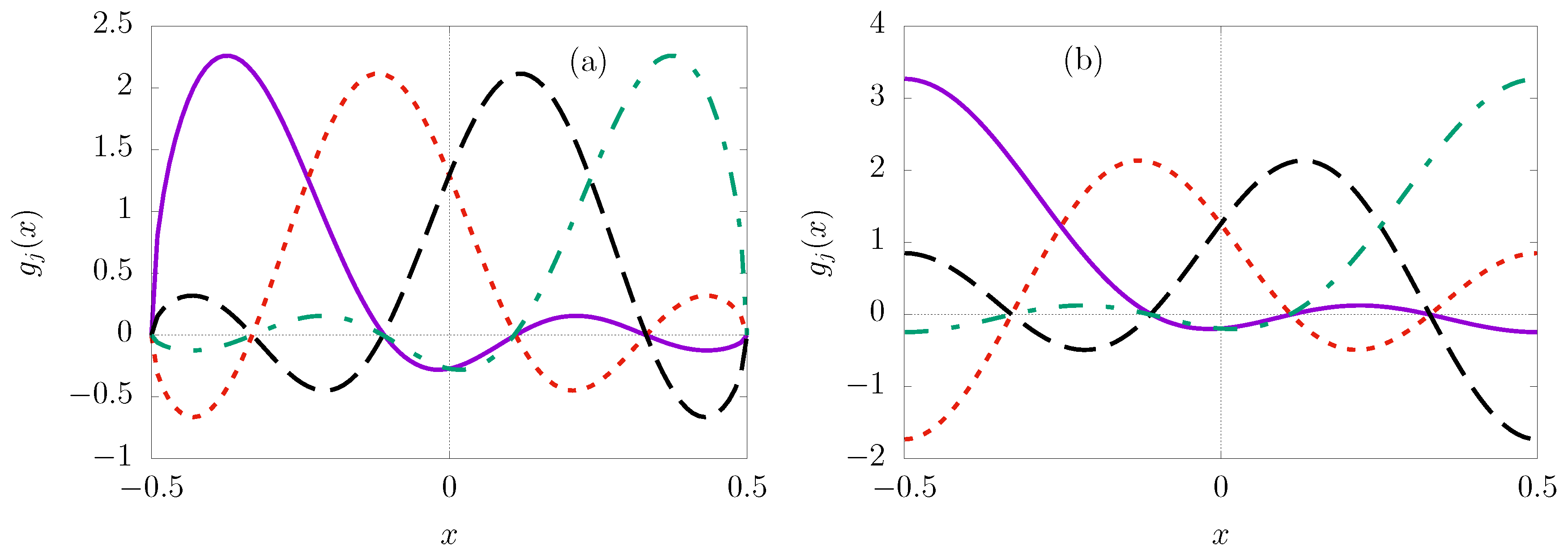
Figure 3.
(a) A plot of the exponential Lagrange-Legendre functions for . (b) Comparison of the function in (a) and its scaled version for .
Figure 3.
(a) A plot of the exponential Lagrange-Legendre functions for . (b) Comparison of the function in (a) and its scaled version for .
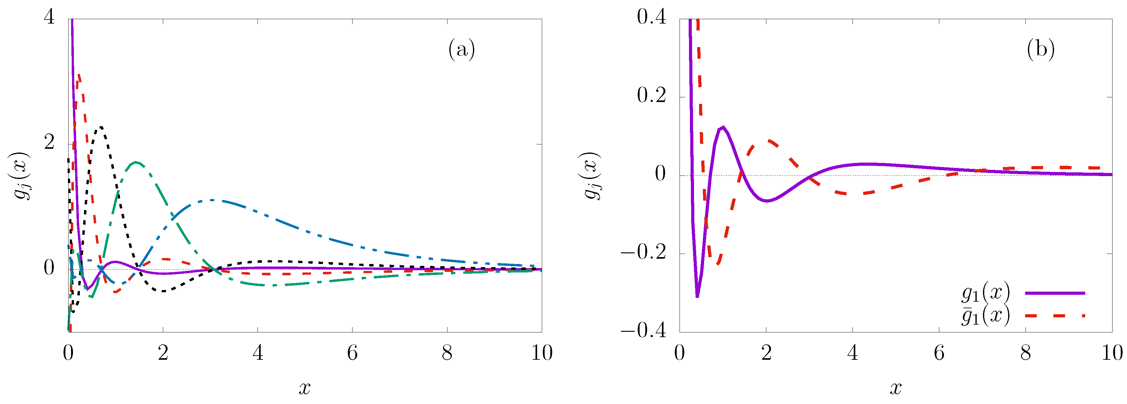
Figure 4.
Plots of the exponential Lagrange-Chebyshev functions (a) of the first kind and (b) of the second kind, for .
Figure 4.
Plots of the exponential Lagrange-Chebyshev functions (a) of the first kind and (b) of the second kind, for .
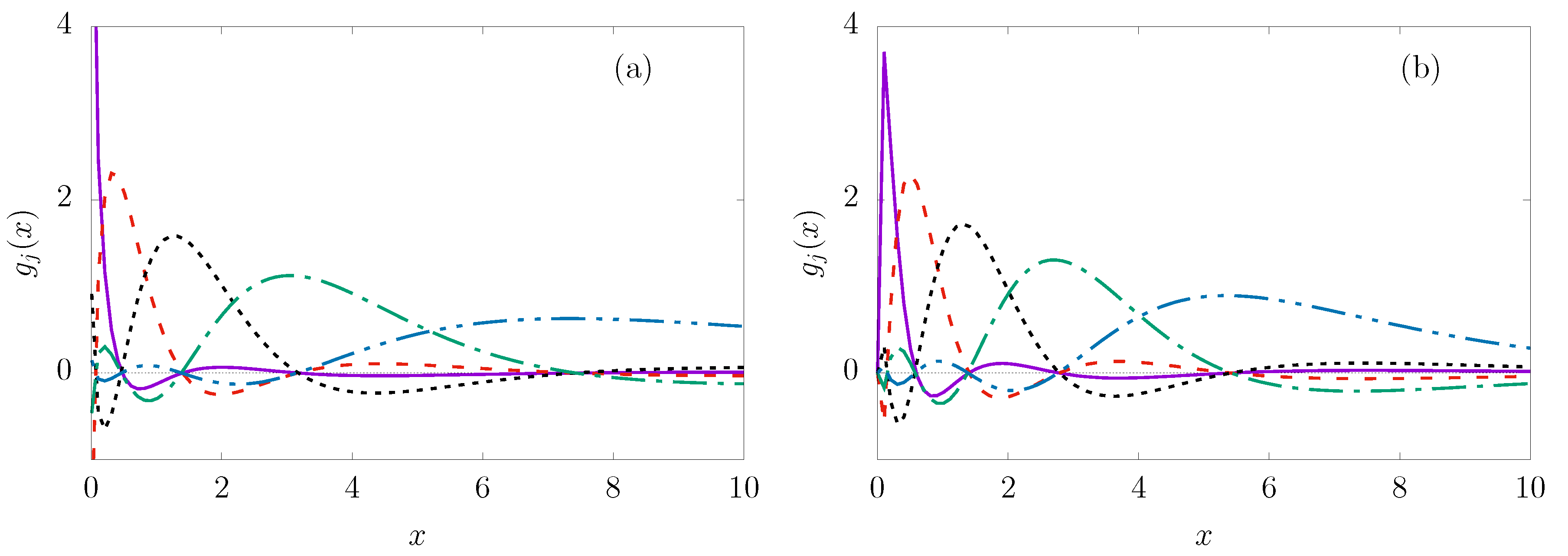
Figure 5.
Plot of the indicated special cases in (a), (b), and (c) of the hyperbolic Lagrange-Jacobi functions for . (d) Comparison of the functions in (a), (b), and (c).
Figure 5.
Plot of the indicated special cases in (a), (b), and (c) of the hyperbolic Lagrange-Jacobi functions for . (d) Comparison of the functions in (a), (b), and (c).
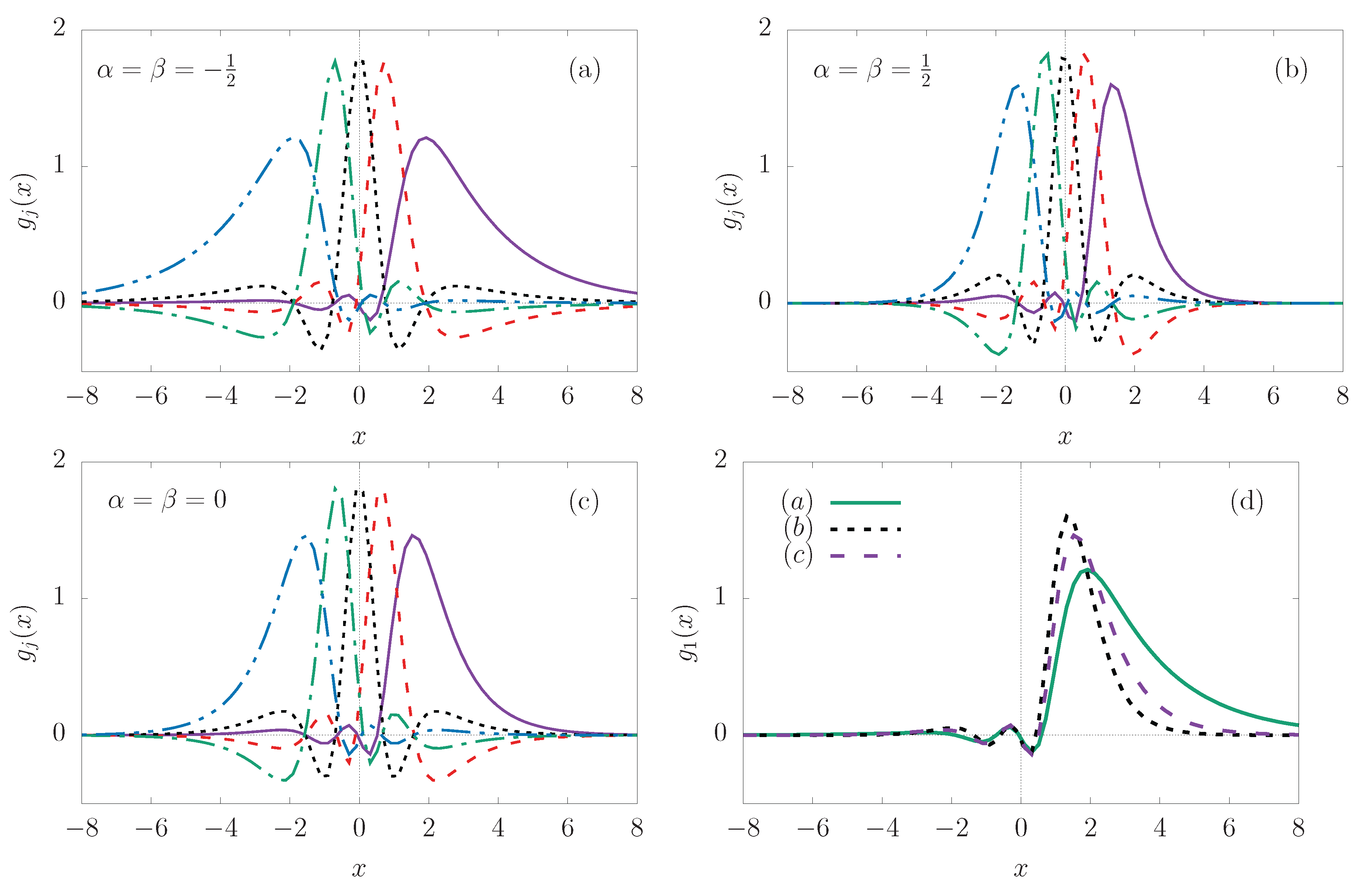

Table 1.
The deference between the numerical and the analytical eigenvalues of the simple harmonic oscillator for the states , , , and at different basis sizes N, with fm. The notation is used.
Table 1.
The deference between the numerical and the analytical eigenvalues of the simple harmonic oscillator for the states , , , and at different basis sizes N, with fm. The notation is used.
| N | |||||
|---|---|---|---|---|---|
| 20 | 8.86(-08) | 2.28(-03) | 8.19(-02) | 1.71(-01) | |
| 30 | 1.27(-14) | 5.34(-11) | 8.82(-07) | 9.04(-04) | |
| 40 | 0.00(00) | 6.66(-16) | 1.28(-11) | 1.05(-07) | |
| 50 | 0.00(00) | 1.33(-15) | 1.20(-11) | 9.82(-08) | |
| 20 | 1.67(-07) | 4.05(-02) | 4.26(-02) | 1.90(-01) | |
| 30 | 0.00(00) | 9.17(-10) | 8.11(-07) | 6.44(-02) | |
| 40 | 9.21(-15) | 3.11(-15) | 1.34(-13) | 3.45(-02) | |
| 50 | 1.42(-14) | 6.66(-16) | 1.19(-13) | 4.58(-09) | |
| 20 | 3.58(-08) | 1.33(-03) | 6.26(-02) | 1.34(-01) | |
| 30 | 2.00(-15) | 1.73(-11) | 3.27(-07) | 4.89(-04) | |
| 40 | 1.42(-14) | 1.67(-15) | 2.17(-11) | 1.76(-07) | |
| 50 | 1.89(-14) | 5.11(-15) | 1.85(-11) | 1.49(-07) |
Table 2.
The relative errors , expressed as , of the calculated eigenvalues of the first four odd states of the Morse potential as a function of the basis size N with , and for the (a) and (b) cases of the exponential Lagrange-Jacobi functions.
Table 2.
The relative errors , expressed as , of the calculated eigenvalues of the first four odd states of the Morse potential as a function of the basis size N with , and for the (a) and (b) cases of the exponential Lagrange-Jacobi functions.
| N | |||||
|---|---|---|---|---|---|
| (a) | 8.32 (-03) | 1.79 (-01) | 2.95 (-01) | 4.71 (-01) | |
| 20 | (b) | 9.33 (-03) | 3.20 (-02) | 3.42 (-01) | 5.29 (-01) |
| (c) | 6.78 (-03) | 2.87 (-03) | 2.51 (-01) | 4.15 (-01) | |
| (a) | 1.75 (-05) | 1.21 (-03) | 1.62 (-03) | 5.58 (-02) | |
| 30 | (b) | 3.24 (-05) | 8.83 (-04) | 1.24 (-02) | 3.32 (-02) |
| (c) | 7.13 (-06) | 1.12 (-03) | 6.23 (-03) | 5.94 (-02) | |
| (a) | 3.95 (-09) | 3.77 (-07) | 2.45 (-05) | 8.22 (-04) | |
| 40 | (b) | 4.54 (-09) | 1.70 (-07) | 7.31 (-05) | 1.63 (-03) |
| (c) | 2.67 (-09) | 5.06 (-07) | 3.70 (-06) | 1.57 (-04) | |
| (a) | 6.61 (-14) | 2.58 (-11) | 3.46 (-09) | 2.00 (-07) | |
| 50 | (b) | 6.19 (-11) | 1.28 (-08) | 1.02 (-06) | 2.41 (-05) |
| (c) | 4.48 (-14) | 2.05 (-11) | 2.83 (-09) | 1.48 (-07) | |
| (a) | 7.97 (-16) | 1.62 (-15) | 6.54 (-15) | 9.90 (-13) | |
| 60 | (b) | 1.80 (-12) | 3.06 (-09) | 8.44 (-08) | 5.70 (-06) |
| (c) | 1.59 (-16) | 2.64 (-15) | 1.10 (-14) | 9.07 (-13) |
(a) , (b) , and (c) , .
Table 3.
The relative errors of the calculated eigenvalues of the first four odd states of the one-dimensional harmonic oscillator as a function of the basis size N of the hyperbolic Lagrange-Jacobi functions at a fixed .
Table 3.
The relative errors of the calculated eigenvalues of the first four odd states of the one-dimensional harmonic oscillator as a function of the basis size N of the hyperbolic Lagrange-Jacobi functions at a fixed .
| N | |||||
|---|---|---|---|---|---|
| (a) | 8.49 (-10) | 3.30 (-07) | 3.28 (-05) | 8.50 (-04) | |
| 20 | (b) | 7.82 (-09) | 6.18 (-07) | 1.01 (-05) | 9.29 (-04) |
| (c) | 2.71 (-09) | 3.93 (-07) | 2.22 (-05) | 3.86 (-04) | |
| (a) | 3.20 (-14) | 8.22 (-12) | 9.44 (-10) | 4.92 (-08) | |
| 30 | (b) | 5.09 (-14) | 9.72 (-12) | 9.89 (-10) | 4.51 (-08) |
| (c) | 1.48 (-15) | 9.33 (-13) | 1.95 (-10) | 1.22 (-08) | |
| (a) | 3.26 (-15) | 7.61 (-16) | 4.81 (-14) | 6.01 (-12) | |
| 40 | (b) | 7.11 (-15) | 1.27 (-16) | 1.25 (-13) | 9.71 (-12) |
| (c) | 4.14 (-15) | 1.65 (-15) | 3.04 (-14) | 1.05 (-12) | |
| (a) | 7.11 (-15) | 3.43 (-15) | 2.42 (-15) | 4.74 (-15) | |
| 50 | (b) | 1.48 (-16) | 2.54 (-16) | 4.84 (-16) | 7.11 (-16) |
| (c) | 7.11 (-15) | 1.02 (-15) | 2.91 (-15) | 4.74 (-16) | |
| (a) | 1.05 (-14) | 5.08 (-15) | 5.17 (-15) | 5.92 (-16) | |
| 60 | (b) | 4.74 (-15) | 6.09 (-15) | 1.61 (-15) | 1.89 (-15) |
| (c) | 1.05 (-14) | 5.08 (-15) | 5.17 (-15) | 5.92 (-16) |
(a) , (b) , and (c) .
Disclaimer/Publisher’s Note: The statements, opinions and data contained in all publications are solely those of the individual author(s) and contributor(s) and not of MDPI and/or the editor(s). MDPI and/or the editor(s) disclaim responsibility for any injury to people or property resulting from any ideas, methods, instructions or products referred to in the content. |
© 2026 by the authors. Licensee MDPI, Basel, Switzerland. This article is an open access article distributed under the terms and conditions of the Creative Commons Attribution (CC BY) license (http://creativecommons.org/licenses/by/4.0/).
Copyright: This open access article is published under a Creative Commons CC BY 4.0 license, which permit the free download, distribution, and reuse, provided that the author and preprint are cited in any reuse.


