
Submitted:
06 January 2026
Posted:
07 January 2026
You are already at the latest version
Abstract
The seemingly endless expanse of the sky might suggest that it could support a large volume of aerial traffic with minimal risk of collisions. However, mid-air collisions do occur and are a significant concern for aviation safety. Pilots are trained in scanning the sky for other aircraft and maneuvering to avoid such accidents, which is known as the basic see-and-avoid principle. While this method has proven effective, it is not infallible because human vision has limitations, and pilot performance can be affected by fatigue or distraction. Despite progress in electronic conspicuity (EC) systems, which effectively increases visibility of aircraft to other airspace users, their utility as collision avoidance systems remains limited. This is because they are recommended but not mandatory in uncontrolled airspace, where most mid-air accidents occur, so other aircraft may not mount a compatible device or have it inactive. Besides, their use carries some risks, such as over-focusing on them. In response to these concerns, this paper presents evidence on the utility of using an optical flow-based obstacle detection system that can complement the pilot and electronic visibility in collision avoidance, but that, contrary to them, neither gets tired as the pilot nor depends on what other aircraft mount, as with EC devices. The current investigation demonstrates that the proposed optical flow-based obstacle detection system meets or exceeds the critical minimum time required for pilots to detect and react to flying obstacles using a mid-air collision simulator in various test environments.
Keywords:
mid-air collision
; flying obstacle detection
; computer vision
; optical flow
; pilot assistance
; simulator
; safety
1. Introduction
Although the sky may seem so big that the probability of two planes colliding in the air is too small to worry about, the truth is that this type of accident does occur. Congestion of uncontrolled airspaces, due to the growth of general aviation (GA) -and, especially, light sport and micro/ultralight aircraft- on the one hand, and the increase in drone operations on the other, contributes to a higher risk of these accidents [1].
Mid-air collisions are a major concern to aviation safety agencies around the world. An example is the EASA (European Union Aviation Safety Agency) that, in its Annual Safety Review 2024 on GA, which analyzes the year 2023, highlights that 68 people died in small aircraft accidents, the main causes being mid-air collisions and loss of control in flight [2]. The United States’ FAA (Federal Aviation Administration) also provides some guidance on avoiding mid-air collisions in recent updates of the Airplane Flying Handbook (AFH). According to the AFH, “most mid-air collision accidents and reported near mid-air collision incidents occur in good VFR weather conditions and during the hours of daylight”, and “most of these accident/incidents occur within 5 miles of an airport and/or near navigation aids” [3].
To prevent such accidents, pilots are instructed to visually scan the skies for potential threats -when weather conditions permit [4]-, and be prepared to maneuver to avoid a collision [5]. This “see-and-avoid” method requires pilots to divide their attention not only outside the cockpit, between actively scanning for other traffics while maintaining situational awareness through visual cues used for navigation, but also between outside and inside the cockpit, checking instruments and flying the aircraft. As a general recommendation, pilots should prioritize visual observation during flight, spending approximately 80% of their time observing their surroundings, and up to 20% to instrument monitoring, with no more than 5 seconds inside the cockpit at a time. A common scanning pattern employed by pilots involves dividing the horizon into nine distinct regions or sectors and dedicating 1-2 seconds to each one. However, this approach has its limitations: it prevents the pilot from simultaneously scanning their entire field of view, thereby increasing the risk that a potential threat might be overlooked while attention is focused on another sector. Besides, not only focus is limited but also range, as human vision can detect and recognize objects only up to approximately 2 nautical miles (3704 meters), under ideal weather conditions [6].
Concern over these accidents is transforming the "see-and-avoid" principle to "see-and-be-seen". There are two types of visibility: passive, with paint and lighting; and active, with electronic systems that transmit to surrounding aircraft and ATC (Air Traffic Control). The latter type, known as electronic conspicuity (EC) [7], provides not only electronic visibility to other aircraft, but also greater situational awareness for the pilot, thus improving flight safety by helping to reduce the risk of collisions in increasingly congested skies.
Above FL150 (Flight Level 150, or 15,000 feet), in controlled space, systems such as radar, secondary surveillance radar (SSR) querying transponders (XPDR), Traffic Collision Avoidance System (TCAS) and, more recently, Automatic Dependent Surveillance-Broadcast (ADS-B) resolve potential conflicts related to the location and separation between aircraft [1]. However, it is known that nearly all mid-air collisions occur at low altitude [8]. Thus, below that FL150, most general and sport aviation aircraft operate in uncontrolled airspace, and there is a greater variety of technologies to provide visibility, adding to the previous systems others such as FLARM (Flight Alarm https://flarm.com/), SafeSky (https://www.safesky.app/) and ADS-L (light version of ADS-B).
However, these technologies should be a complement, not a substitute, as their misuse can lead to risks such as: distraction, due to over-focusing on the equipment; dependency, due to neglecting traditional navigation techniques; device, software, or battery failures, or overheating that can cause a fire; outdated information, which causes the pilot to ignore current hazards in the airspace; and poor placement, which blocks the pilot’s vision or interferes with their controls. Besides, EC devices are not mandatory in uncontrolled airspaces yet, thus other aircraft may not be electronically visible because they do not mount a compatible device, this is switched off or it is not working [9].
Given the above risks, pilots should keep their traditional skills well-honed. To illustrate the importance of this, [10] describes a situation where two PA-28 aircraft traveling at 90 knots fly directly to each other; notably, the other aircraft remains almost imperceptible until the distance between them falls below 500 meters, then the threat blooms in size in the pilot’s retina, leaving only 5 seconds to recognize and take action before impact. However, as explained in [11], the process of identifying and responding to a flying obstacle typically takes longer and involves two time-critical steps. First, the pilot must visually detect the hazardous object and be aware of its collision course, which takes 6.1s. Second, the pilot must decide what to do and physically react, which, also considering the aircraft’s lag time, adds 6.4 s. Thus, the entire process takes 12.5 s. In addition, the see-and-avoid method has several other limitations. It may be physically impossible for pilots to detect an approaching aircraft under certain flight conditions, such as climbing or descending within an airport traffic pattern. Moreover, pilot vision’s clarity may be influenced by other circumstances, such as light reflected by the object or the object’s contrast with the surrounding environment [12].
The objective of this work was to evaluate the performance of a proposed solution aimed at enhancing human pilot reaction capabilities in mid-air collision avoidance. To this end, a 3D simulation environment was developed to replicate real-world scenarios. Unlike approaches that depend on deep learning [13,14,15,16], such as the one proposed by [17,18], the method presented here utilizes traditional optical flow-based techniques [19,20], which have already demonstrated effectiveness in applications involving flying machines, including ego-motion estimation [21], path planning [22], and attitude estimation [23]. A key advantage of using traditional optical flow lies in its independence from large training datasets [24], which are particularly challenging to obtain for scenarios involving mid-air collisions [25,26].
The proposed detection system employs real-time image processing, from a single onboard camera, to calculate the optical flow through consecutive video frames and detect potential obstacles based on the differences with neighbour pixels [27]. When they are detected, the system frames them to bound the threats, allowing the pilot to assess them and execute evasive maneuvers such as altering altitude or course. The intended final users are pilots flying aircraft -with or without EC aids- in uncontrolled airspaces, low and slow, where risk of a mid-air collision is higher.
It is worth noting that to effectively manage the complexities of flight operations and minimize the risk of accidents or errors, pilots must take into account several essential factors, including fatigue, stress, distraction, emotional influences, sleep deprivation, aging, and physical health [29]. Our approach is immune to these cognitive and physiological limitations and doesn’t depend on the avionics of other aircraft, allowing for more consistent and reliable decision making by the pilot. In addition, we will demonstrate that this computer vision-based proposal is capable of detecting potential threats at a greater distance than is possible for humans, giving pilots enough time to take evasive action and avoid collisions. Thus, the contribution of this work can be summed up as follows:
- A novel computer vision-based collision avoidance system is presented that complements human pilots in preventing mid-air collisions by providing timely alerts for timely response.
- The system integrates a suite of sophisticated techniques to avoid mid-air collisions: light morphological filters, optical flow, focus of expansion, and Density-Based Spatial Clustering of Applications with Noise (DBSCAN).
- The system’s performance is compared with data available about human’s ability to detect flying obstacles during flight, in order to evaluate the effectiveness of our proposed mid-air collision detection algorithm.
The remainder of the paper is organized as follows. Section 2 describes the proposed method for early detection of flying obstacles by optical flow and explains the experimental setup. The results are given in Section 3, divided into subsections that address the different test scenarios. Finally, Section 5 presents the most important conclusions of the work.
2. Material and Methods
The proposed mid-air obstacle detection system is a multi-platform application that runs on various operating systems, including Windows, MacOS, and Linux distributions. The software was developed using the .NET 7.0 SDK with C# as the primary programming language. The computer vision algorithms for obstacle detection used the Emgu.CV v4.7.0 library. In the following subsections, details of these algorithms are given, followed by an explanation of the simulator developed to test the detection system, and ending with the experimental setup and procedure.
2.1. Detection of Flying Obstacles
Building on previous studies using similar techniques such as morphological operations and optical flow, our approach uniquely relies on the analysis of optical flow vectors to detect potential threats. By examining the direction of these vectors in specific areas, we identify anomalies that may indicate an approaching obstacle. The results presented in our previous publication [30] show promising performance in filtering out environmental noise and detecting possible obstacles. As a more detailed explanation of the proposed process is given in that paper, what follows next is just a summary of it for the sake of completeness of the simulation and the analysis that are presented here.
Thus, our detection system takes, as input, images captured by a monocular camera during flight [31], and obtains as ouput the obstacles identified through a multi-stage process (Figure 1). First, the morphological close-minus-open (CMO) filter [32] [33] is applied to the image to reduce the noise generated by clouds, ground, and sun, in order to facilitate the detection of flying obstacles in the next stages (Figure 1, box (a)). The algorithm of the CMO filter computes the difference between morphological closing and opening operations on an input scene. Dilation and erosion are the two basic grayscale morphological operations that make up both closing and opening actions. The dilation operation expands or thickens objects in binary images, while erosion reduces the size of foreground objects. Specifically, to perform an opening, erosion is applied first ,followed by dilation, while a closing is done in the reverse order, dilation is applied first, followed by erosion. The closing operation effectively removes all dark objects or regions smaller than a certain size, while the opening operation achieves the opposite effect by removing all light objects or regions below a certain threshold [34]. With these operations, we expect not only to reduce the noise, but also to separate elements and consolidate separated entities for the next step.
Then, motion vectors are obtained by comparing consecutive frames using the Gunnar-Farnebäck (GF) dense optical flow method [35] (Figure 1, box (b)). Optical flow refers to the motion of objects or the camera between consecutive frames in a video sequence, represented as a 2D vector field [27]. Each vector in this field represents the displacement of points from one frame to another, providing information about the direction and magnitude of the motion. Using GF’s optical flow, a list of 2D vectors is obtained from which the trajectory of the aircraft and the detection of potential obstacles can be inferred.
The intersection points of the optical flow vectors allow us to calculate the Focus of Expansion (FOE), which represents the point in the image plane where the 3D velocity vector describing the camera motion intersects the projection plane (Figure 1, box (c)). The FOE is a critical component of various applications, including time-to-impact estimation and motion control systems, such as collision warning systems and obstacle avoidance mechanisms [36]. In scenarios where environmental motion is aligned with the FOE, misaligned motion vectors indicate the presence of an obstacle. The system detects obstacles by analyzing increased noise in the environment and its effect on focus estimation (FE). To compute FE, the image is divided into four quadrants and motion vectors within each quadrant are analyzed. Intersections between these vectors are identified, resulting in a set of points that, after averaging to reduce noise, define the FOE. The system then filters out nonconforming motion vectors using the approximated FOE.
Finally, the remaining vectors are clustered using the DBSCAN algorithm (Figure 1, box (d)). DBSCAN is an unsupervised clustering algorithm that groups data points based on their proximity to each other, while also identifying outliers as those that are far from any cluster. In our system, each cluster represents the location of a potential approaching obstacle. The process begins by selecting a random point and searching for nearby points within a specified distance (EPS). If it finds at least min_samples points within this radius, DBSCAN forms a cluster around them. It processes all the data until the iterative process is complete [37]. One of the key advantages of DBSCAN is its ability to detect clusters of various shapes and sizes, as long as there are enough points within the EPS. In addition, it can identify outliers that are significantly different from the rest of the data. As an unsupervised algorithm, it doesn’t require pre-labeled data or a predetermined number of clusters [38].
2.2. Description of the Simulator
The authors created a 3D mid-air collision simulator to evaluate the performance of our proposal. This allowed us to quantify how long, before a potential collision, the system would be able to detect a flying obstacle and, therefore, how much reaction time the pilot would have after issuing the threat warning. Our simulator included two aircraft: one equipped with the camera that feeds our mid-air collision detection system, and another that served as a flying obstacle.
The simulator was designed to allow for flexible testing by allowing the user to customize various parameters, such as altitude, speed and heading of each aircraft, thus shaping different scenarios. In particular, we were interested in reproducing three common aircraft proximity (airprox) scenarios where a mid-air collision or near mid-air collision can occur. These are based on the right of way rules in the air, and that statistics have demonstrated to be typical mid-air collision scenarios [6,11]. These scenarios are (Figure 2): overtaking or close-in (Figure 3), approaching head-on (Figure 4), and crossing (Figure 5). For the latter two sscenarios, the side from which the obstacle approaches (left or right) is also configurable. The initial distance between the two airplanes and the altitude difference (higher, same, lower) at the start of the simulation may also be specified by the user. In addition, both aircraft speeds are adjustable, which is particularly important for the close-in scenario where speed difference is critical. All these customizable parameters allow tailored test configurations to meet specific research objectives.
The simulator continuously feeds generated frames to the collision avoidance system for flying obstacle detection, enabling real-time monitoring and response. When the system detects obstacles, their position is reported back to the simulator, which then visualizes this information as a red rectangle on the screen (as shown, for instance, in Figure 3).
As the simulation runs, key metrics are recorded for later evaluation and analysis. These metrics include the distance between the two airplanes in each frame, providing valuable insight into their relative positions. For the purpose of calculating this distance, each airplane is represented by a single 3D point in space. The total duration from the start to the end of the simulation is also a critical metric. Specifically, simulation completion occurs when the minimum distance between the aircraft is reached, marking the point of closest approach in the scenario. By tracking this elapsed time, we can evaluate how much warning the system would have provided to the pilot to avoid the obstacle.
2.3. Experimental Setup
The 3D model used for the two aircraft in the simulations carried out for this experiment is the Cessna 172s (Figure 6), one of the most popular aircraft in the world [39]. Only one of these two models is seen in the pictures, the one that plays the role of flying obstacle or threat, as the other is the one that mounts the camera of the simulation. The Cessna 172s has an overall length of 27’2” (8.28 m) -which is relevant data for the crossing scenario-, wingspan of 36’ (11 m) -relevant for close-in and head-on scenarios-, and height of 8’11” (2.72 m) -relevant for all scenarios-. In this experiment, the two aircraft are flying at a speed of 124 knots (approx. 230 km/h), which is the typical cruising speed of a Cessna 172s [39], except in the close-in scenario, where the threat flies relatively slower to allow the Cessna mounting the camera to reach it. In each test configuration, the altitude at which the threat travels is varied: 1065, 1000, and 935 feet (ft), referred to as higher, same, and lower levels, respectively. We chose 1000 ft as the reference because it is reported that nearly all mid-air accidents occur at or near non-towered airports below that altitude [8].
As for the camera, the simulation aims at reproducing a typical sport camera that the aircraft may mount. A camera like this has a 1/1.9" CMOS sensor with a resolution of 27.6 MP. The lens has a focal length of 35mm and an aperture range of F2.5 with an FOV of 156° in an 8:7 aspect ratio. For video, it can record at 4K resolution with a frame rate of up to 25 fps.
The simulations trials were all executed on the same PC, running Ubuntu 22.04.4 LTS (Jammy Jellyfish), equipped with an AMD Ryzen 5 3600 processor with six cores and twelve threads, and an Nvidia GeForce RTX 4060 graphics card with 8 GB of GDDR6 memory. Each trial provides two key metrics: the detection distance at which the obstacle is identified, and the time to collision before the two aircraft converge. Due to the variability in operations involved, even with the same configuration, it is essential to account for this inherent uncertainty. To ensure the reliability and robustness of their results, the authors repeated each scenario 10 times, calculating mean values for both detection distance and lead time. This approach enables a more comprehensive understanding of the system’s performance under different conditions.
3. Results
The objective of this work was to evaluate the performance of our proposed solution to enhance the human pilot’s reaction capabilities in mid-air collision avoidance. To achieve this goal, the authors developed a 3D simulation environment that mimics real-world scenarios. A series of simulations was run for each approach type at the three available altitudes offered by the simulator to investigate the effect of altitude on detection performance. Specifically, the authors ran 10 trials per configuration. On average, each frame took about 8.66 milliseconds to be processed on the PC described previously, demonstrating efficient performance.
3.1. Close-in Scenarios
In the close-in scenario, the algorithm detects an approaching aircraft traveling in the same direction but at a slower speed than the host aircraft equipped with the proposed system. To evaluate this configuration, the obstacle speed was set relative to the host aircraft cruise speed, which is 124 knots, with reductions of 10% (111.6 kn), 20% (99.2 kn), and 30% (86.8 kn). Three vertical separation conditions were tested: the obstacle was placed at a higher altitude (1065 ft), the same altitude (1000 ft), or a lower altitude (935 ft), while the host aircraft remained at 1000 ft.
As shown in Table 1 and Figure 7, the average time remaining after detection in the close-in scenario decreases with greater speed differences. At a 10% speed reduction, average times are highest across all altitude configurations, with the "same altitude" scenario resulting in the longest time (320.45 s). At 20%, average times drop notably, with the "same altitude" condition again yielding the longest time (178.70 s). At 30%, detection times are the lowest overall, with the "lower altitude" case producing the shortest average time (128.26 s). The consistent trend of longer times in the "same altitude" scenario suggests that the system detects aircraft more readily at the same flight level. In addition, standard deviations decline with increasing speed reduction, indicating improved consistency in detection.
Table 2 and Figure 8 present the corresponding distances at which the threat is detected for this close-in scenario. For each speed difference, the "same altitude" condition yields the longest average detection distance, peaking at 1839.60 m at a 10% speed reduction. This supports the finding that the system is more effective when both aircraft are at the same altitude. In contrast, the "lower altitude" obstacle consistently results in the shortest detection distances. Although detection distances increase as the flying obstacle reduces its speed, the differences are not substantial, indicating relatively consistent system performance across configurations.
Even in the least favorable scenario —30% speed reduction with the obstacle at a higher altitude— the system detects the intruder approximately 2 minutes and 1603 meters before a potential collision. This lead time provides sufficient margin for the pilot to execute an evasive maneuver.
3.2. Head-on Scenarios
The head-on scenario simulates two aircraft flying toward each other at a constant speed of 124 knots. The left and right variants refer to the side of the visual field from which the approaching obstacle enters. To evaluate the influence of relative altitude on detection performance, both approach directions were tested across three vertical configurations: higher, same, and lower altitude relative to the observer aircraft.
As shown in Table 3 and Figure 9, the system consistently detects obstacles earlier when the obstacle is located at a higher altitude. For both left and right approaches, the longest average remaining times were recorded for "higher altitude" obstacles, at 30.15 and 30.49 seconds, respectively. In contrast, obstacles at the same altitude as the aircraft were detected significantly later, with average reaction times of 14.15 seconds (left) and 13.85 seconds (right). Obstacles at lower altitudes yielded intermediate values, indicating that detection occurs sooner than for "same altitude" cases, but later than for "higher altitude" obstacles.
The corresponding trends are observed in the reaction distance results, presented in Table 4 and Figure 10. The system detected high-altitude obstacles at the greatest distances 3844.60 meters for left approaches and 3891.50 meters for right. The detection distance dropped markedly when the obstacle was at the same altitude, to approximately 1800 meters. Lower altitude obstacles were detected at intermediate distances of 3060.50 meters (left) and 3136.80 meters (right). These findings suggest that obstacles at or near the aircraft’s altitude produce less noticeable motion, leading to delayed detection and reduced time and space for evasive maneuvers.
In general, the system exhibited the most effective detection when the obstacle was positioned above the aircraft. This performance may be attributed to greater angular displacement and associated visual motion in the optical flow. Future work will focus on enhancing detection capabilities for the same altitude scenarios.
3.3. Crossing Scenarios
In the crossing scenario, the second aircraft was flying perpendicular to the aircraft equipped with our optical flow-based solution. The goal of testing this scenario was to discover the maximum distance at which the system can detect the intruder. For this set of tests, the time represents how long it took for the obstacle, from where it was detected, to be in front of the airplane with the camera onboard.
As shown in Table 5 and Figure 11, on average the system detects obstacles earlier when the obstacle is located at a different altitude, for both left and right approaches, with remaining times after detection that range from 19.26 seconds as maximum in the best case (right-higher) to 14.69 seconds as minimum in the worst case (left-lower). In contrast, threats at the same altitude were detected later, with an average remaining time of 14.43 seconds for the left approach, and 14.66 seconds for the right one. However, looking at the maximum and minimum of the "same-altitude" condition, its range slightly overlap with the results from "right-lower" case. Overall, the results in this scenario spread from 13.74 seconds minimum (right-same) to 19.26 seconds maximum (right-higher), which gives a narrow range, less than 6 seconds.
Table 6 and Figure 12 illustrates that, for obstacles that appear from the left side, the shortest detection distances were observed when the obstacle was at the same altitude, with an average of 1840.28 meters. In contrast, detection distances increased when the obstacle was at a lower altitude, reaching an average of 2504.93 meters, and were longest when the obstacle was at a higher altitude, with an average of 2690.26 meters. A similar trend is visible on the right side, where the average reaction distance for same-altitude obstacles was 1910.54 meters, while higher and lower obstacles elicited longer average distances of 2524.66 meters and 2525.06 meters, respectively.
These results indicate that the system can detect intruders at greater distances, particularly when the intruder is located above or below the aircraft. Obstacles at the same altitude showed the largest standard deviations, particularly for left-side approaches (69.97 meters), indicating less consistent detection in these scenarios. In contrast, responses to higher and lower obstacles were more stable, with standard deviations ranging from 30.62 to 64.77 meters. This is attributed to the optical flow vectors of the intruder more closely aligning with the optical flow patterns generated by the aircraft’s motion in these relative positions.
The simulations generated valuable insight into the performance of our approach, providing metrics for both detection distance and alert time for potential collisions. Specifically, each simulation generated data on the distance at which the flying obstacle was detected, as well as the time that would provide for the pilot to react to a dangerous aircraft proximity scenario.
4. Discussion
While previous studies have demonstrated the effectiveness of various algorithm combinations in detecting flying obstacles, e.g., [36,40,41], to the best of our knowledge, no existing work has simultaneously applied the CMO filter, optical flow, FOE, and DBSCAN algorithms to achieve this goal. This absence presents an opportunity for innovative research that leverages the strengths of each algorithm to develop more robust obstacle detection methods as is the case in the present work.
Compared to other approaches to collision avoidance using computer vision, our proposal has several advantages. For example, a processing pipeline has been proposed that detects and evaluates potential collision-course targets from aerial scenes captured by optical cameras, enabling a vision-based sense-and-avoid (SAA) system [42]. This SAA system uses eight feature detectors and three spatiotemporal visual cues to identify potential collisions. Several metrics, including a percentage of detected targets, false positive rates, and accuracy rates, evaluate the performance of the pipeline. The results demonstrate high accuracy in detecting collision course targets with low false positive rates. However, the use of multiple cameras increases the processing time requirements, necessitating more powerful hardware to support real-time operation. In contrast, our approach shows promising results using a single monocular camera with a hardware setup below US $1000.
Deep learning has also been applied to obstacle detection tasks, with notable success in vision-based mid-air collision avoidance for small UAVs. A very recent approach presents a deep learning-based system that uses computer vision to detect objects in flight and generate evasive maneuvers [26]. This method was evaluated under various conditions, including different distances, angles, and speeds of the detected object. The results demonstrated high accuracy in detecting mid-air objects, with successful collision avoidance achieved in approximately 90% of the simulated scenarios. However, some limitations were observed: estimation errors increased when the size of the target UAV differed from that used in the study. In addition, the detection range was insufficient to meet the requirements of UAV Traffic Management (UTM) [28,43]. Notably, our approach relies on real-time processing and does not require pre-trained datasets or specific object models, making it more reliable in unexpected situations.
Although the current approach does not inherently limit detection to a single flying obstacle, this work primarily evaluated the algorithm’s performance in identifying a single target compared to human capabilities. Through testing under different scenarios, we gained valuable insight into the performance of the proposed approach. The tests revealed the maximum distance at which our system can successfully detect a flying obstacle, as well as the time elapsed from detection until the obstacle reaches our aircraft.
Notably, once a flying obstacle enters the field of view, the system can identify it almost instantly. The maximum detection distance varies depending on the altitude of the obstacle, but we have found that it is typically around 2360 m (approx. 1.27 NM). Indeed, the system’s detection capabilities depend on the type and speed of the approach and can detect obstacles at distances from approximately 0.8 NM (1482 m) to 2 NM (3704 m). In most cases, this is less than the distance at which a human pilot can visually detect an obstacle in optimal conditions. However, it’s essential to note that our system evaluates the entire field of vision simultaneously, whereas pilots can only assess a portion at a time. Indeed, during the 1-2 seconds that a pilot takes to scan one of the nine regions they may divide the horizon in front of them, the detection system would have scanned the camera’s field of view from side to side a number of times. This ensures significant assistance to the pilot in the event of a collision hazard.
Moreover, after testing our mid-air collision avoidance system using the 3D simulator, the authors are confident that the proposed algorithm can warn pilots of approaching obstacles in most cases with more than 12.5 seconds of warning, which is the typical recognition and reaction times[11], providing sufficient time for evasive maneuvers. As mentioned above, the crossing scenarios are particularly well suited to our system because they allow us to detect obstacles with high accuracy.
Thus, the proposed system has several advantages over the traditional “see-and-avoid” human-based method. Unlike pilots who must focus on one section of their visual field at a time, our system can analyze its entire visual field simultaneously. This allows for faster and more accurate detection of potential collisions, reducing the risk of accidents. Secondly, our system is not susceptible to fatigue or visual problems, which are common limitations faced by pilots. For instance, pilots may experience visual overload in high-stress situations, leading to decreased situational awareness and increased reaction time [3]. In contrast, the proposed system can operate continuously without fatigue, ensuring consistent performance even during prolonged periods of intense activity.
Furthermore, our proposed system has the potential to improve overall aviation safety. By detecting potential collisions earlier than human pilots, we can reduce the risk of accidents and minimize damage in the event of a collision [44]. In addition, our system’s potential to analyze multiple aircraft trajectories simultaneously allows for more effective management of air traffic, reducing congestion and increasing efficiency. However, there are some limitations to consider. For example, our system relies on accurate sensor data, which can be affected by factors such as weather conditions or equipment malfunctions. In this sense, it is important to recognize that the ultimate performance and effectiveness of the system will depend on the quality of the imagery and the characteristics of the environment. Despite these limitations, we believe that our mid-air collision avoidance system has great potential to help prevent accidents and improve aviation safety.
Future work will build on these results by investigating the algorithm’s performance in other typical mid-collision scenarios, such as landing at airports or collisions with Unmanned Aircraft Systems (UAS) [11]. Besides, since the algorithm also has the ability to detect and track multiple obstacles, we could test its performance in the above scenarios but involving more than one threat at a time. Moreover, future research directions could leave behind the simulator and the computer-generated images to test the proposed system with real video, first running on a PC as we did for this experiment but with recorded video footage, then on a laptop with the purpose of taking it onboard an aircraft connected to a real camera mounted on the plane. Ultimately, this roadmap would lead to the development of a lightweight version of the system that could run on portable/mobile solutions onboard any light aircraft.
5. Conclusions
In this paper, the authors have demonstrated the potential of using an optical flow-based solution in detecting flying obstacles, and how this technology can effectively complement pilots in the task of spotting threats and avoiding mid-air collisions, the “see-and-avoid” method. From our simulations of typical mid-air collisions scenarios, results have shown that the flying obstacle is detected with enough distance and time for the pilot to take action and avoid the collision. Our approach does not suffer from the limitations of human perception and performance, such as attention deficits or visual fatigue, which can be critical when every second counts. Compared to other computer vision methods based on pre-trained models, our proposal does not need such models and thus do not depend on their quality. In addition, in comparison to electronic conspicuity solutions, our proposal is independent of what other aircraft are mounting, nor does it rely on communication between them.
Future work would, as stated in the discussion section, test the performance of the proposed system in new scenarios and add more complexity to them with multiple threats and UAS. Besides, research on UAS detection could also leverage on another major concern in aviation safety: bird strikes. Indeed, large birds are even bigger than many UAS, such as vultures and eagles, which have an wingspan of 2 meters or more. We are also working on the development of innovative interfaces for mid-air collision avoidance systems, in particular using augmented reality glasses that provide pilots with timely alerts when obstacles approach [6]. Thus, we expect to integrate such interface into the detection system in the near future. Beyond that, and with a portable/mobile version of our system that could be taken onboard an aircraft, other research and development opportunities would open, for instance the integration with existing electronic conspicuity solutions, such as SafeSky or ADS-L. This way, traffic information from these other sources could confirm flying obstacles detected by our independent CV-based solution, and our system could share its information on detected threats that are not electronically visible.
Author Contributions
Daniel Vera-Yanez: Data curation, Investigation, Methodology, Writing – original draft, Writing - review & editing. António Pereira: Conceptualization, Resources, Supervision, Validation, Writing - review & editing. Nuno Rodrigues: Conceptualization, Formal analysis, Methodology, Writing - review & editing. José P. Molina: Conceptualization, Validation, Supervision, Writing - review & editing. Arturo S. García: Conceptualization, Investigation, Methodology, Writing - review & editing. Antonio Fernández-Caballero: Conceptualization, Resources, Supervision, Validation, Writing - review & editing.
Funding
Grant EQC2019-006063-P funded by Spanish MICIU/AEI/10.13039/501100011033 and by “ERDF A way to make Europe”. Grant 2022-GRIN-34436 funded by Universidad de Castilla-La Mancha and by “ERDF A way of making Europe”. This work was also partially supported by the Portuguese FCT-Fundação para a Ciência e a Tecnologia, I.P., within project UIDB/04524/2020 and by the project DBoidS - Digital twin Boids fire prevention System: PTDC/CCI-COM/2416/2021.
Institutional Review Board Statement
Not applicable.
Informed Consent Statement
Not applicable.
Data Availability Statement
The data presented in this study are available on request from the corresponding author.
Conflicts of Interest
The authors declare no conflicts of interest.
Abbreviations
The following abbreviations are used in this manuscript:
| ADS-B | Automatic Dependent Surveillance Broadcast |
| CMO | Close-Minus-Open |
| EC | Electronic Conspicuity |
| FLARM | FLight alARM |
| FOE | Focus of expansion |
| GF | Gunnar–Farnebäck |
| HMM | Hidden Markov Model |
| ROS | Robot Operating System |
| SSR | Secondary Surveillance Radar |
| TCAS | Traffic Collision Avoidance System |
| UAV | Unmanned aerial vehicle |
References
- B. Taylor, M. Allen, P. Henson, X. Gao, H. Malik, and P. Zhu, Enhancing Drone Navigation and Control: Gesture-Based Piloting, Obstacle Avoidance, and 3D Trajectory Mapping. Applied Sciences 2025, vol. 15(no. 13), art. 7340. [CrossRef]
- European Union Aviation Safety Agency. Annual Safety Review 2024. Available online: https://www.easa.europa.eu/en/document-library/general-publications/annual-safety-review-2024.
- Federal Aviation Administration. Airplane Flying Handbook, (FAA-H-8083-3C). 2021. Available online: https://www.faa.gov/regulations_policies/handbooks_manuals/aviation/airplane_handbook.
- Goh, J.; Wiegmann, D.; O’Hare, D. Human factors analysis of accidents involving visual flight rules flight into adverse weather. Aviation, Space, and Environmental Medicine 2002, 73(8), 817–822. [Google Scholar]
- Federal Aviation Administration. How to Avoid a Mid Air Collision. Available online: https://www.faasafety.gov/gslac/alc/libview_normal.aspx?id=6851 (accessed on 29 July 2025).
- Á. Torres, J. P. Molina, A. S. García, P. González, Prototyping of augmented reality interfaces for air traffic alert and their evaluation using a virtual reality aircraft-proximity simulator. 2024 IEEE Conference Virtual Reality and 3D User Interfaces, 2024; IEEE; pp. 817–826.
- S. Uzochukwu, I can see clearly now. Microlight Flying Magazine 2019, 11(12), 22–24.
- Turner, T. Mid-Air Strategies. Aviation Safety. 21 September 2022. Available online: https://aviationsafetymagazine.com/risk_management/mid-air-strategies.
- UK Civil Aviation Authority. Investigation into the Human Factors Effects of Electronic Conspicuity Devices in UK General Aviation. 2023. Available online: https://www.caa.co.uk/our-work/publications/documents/content/cap2583/.
- UK Airprox Board, When every second counts. In Airprox Magazine; 2017; pp. 2–3.
- Federal Aviation Administration. Pilots’ role in collision avoidance, Advisory Circular AC 90-48E, Issued 2022-10-20. Available online: https://www.faa.gov/regulations_policies/advisory_circulars/index.cfm/go/document.information/documentID/1041368.
- Morris, C. C. Midair collisions: Limitations of the see-and-avoid concept in civil aviation. Aviation, Space, and Environmental Medicine 2005, 76(4), 357–365. [Google Scholar] [PubMed]
- Shah, S.; Xuezhi, X. Traditional and modern strategies for optical flow: An investigation. SN Applied Sciences 2021, 3, 289. [Google Scholar] [CrossRef]
- M. T. López, M. A. Fernández, A. Fernández-Caballero, J. Mira, A. E. Delgado, Dynamic visual attention model in image sequences. Image and Vision Computing 2007, 25(5), 597–613. [CrossRef]
- A. Fernández-Caballero, M. A. Fernández, J. Mira, A. E. Delgado, Spatio-temporal shape building from image sequences using lateral interaction in accumulative computation. Pattern Recognition 2003, 36(5), 1131–1142. [CrossRef]
- Fernández-Caballero, A.; Mira, J.; Fernández, M. A.; Delgado, A. E. On motion detection through a multi-layer neural network architecture. Neural Networks 2003, 16(2), 205–222. [Google Scholar] [CrossRef]
- Liu, J.; Cui, J.; Ye, M.; Zhu, X.; Tang, S. Shooting condition insensitive unmanned aerial vehicle object detection. Expert Systems with Applications 2024, 246, 123221. Available online: https://www.sciencedirect.com/science/article/pii/S0957417424000861. [CrossRef]
- Yi, S.; Li, J.; Jiang, G.; Liu, X.; Chen, L. Cctseg: A cascade composite transformer semantic segmentation network for uav visual perception. Measurement 2023, 211, 112612. [Google Scholar] [CrossRef]
- Li, X.; He, C.; Tang, Y. Improved modeling and fast in-field calibration of optical flow sensor for unmanned aerial vehicle position estimation. Measurement 2024, 225, 114066. [Google Scholar] [CrossRef]
- Wu, J.; Liu, S.; Wang, Z.; Zhang, X.; Guo, R. Dynamic depth estimation of weakly textured objects based on light field speckle projection and adaptive step length of optical flow method. Measurement 2023, 214, 112834. [Google Scholar] [CrossRef]
- Grabe, V.; Bülthoff, H. H.; Scaramuzza, D.; Giordano, P. R. Nonlinear ego-motion estimation from optical flow for online control of a quadrotor UAV. International Journal of Robotics Research 2015, 34(8), 1114–1135. [Google Scholar] [CrossRef]
- Allasia, G.; Rizzo, A.; Valavanis, K. Quadrotor UAV 3D path planning with optical-flow-based obstacle avoidance. 2021 International Conference on Unmanned Aircraft Systems, 2021; pp. 1029–1036. [Google Scholar] [CrossRef]
- Liu, X.; Li, X.; Shi, Q.; Xu, C.; Tang, Y. UAV attitude estimation based on MARG and optical flow sensors using gated recurrent unit. International Journal of Distributed Sensor Networks 2021, 17(4), 15501477211009814. [Google Scholar] [CrossRef]
- Al-Kaff, A.; Martín, D.; García, F.; de la Escalera, A.; Armingol, J. M. Survey of computer vision algorithms and applications for unmanned aerial vehicles. Expert Systems with Applications 2018, 92, 447–463. [Google Scholar] [CrossRef]
- Preeti, C. Rana, Artificial intelligence based object detection and traffic prediction by autonomous vehicles – a review. Expert Systems with Applications 2024, 255, 124664. [Google Scholar] [CrossRef]
- Lai, Y.-C.; Lin, T.-Y. Vision-based mid-air object detection and avoidance approach for small unmanned aerial vehicles with deep learning and risk assessment. Remote Sensing 2024, 16(5), 756. [Google Scholar] [CrossRef]
- Park, M.-H.; Cho, J.-H.; Kim, Y.-T. Real-Time Optical Flow Estimation Method Based on Cross-Stage Network. Applied Sciences 2023, vol. 13(no. 24), art. 13056. [Google Scholar] [CrossRef]
- Benhadhria, S.; Mansouri, M.; Benkhlifa, A.; Gharbi, I.; Jlili, N. VAGADRONE: Intelligent and Fully Automatic Drone Based on Raspberry Pi and Android. Applied Sciences 2021, vol. 11(no. 7), art. 3153. [Google Scholar] [CrossRef]
- Campbell, R. D.; Bagshaw, M. Human Performance and Limitations in Aviation; John Wiley & Sons, 2002. [Google Scholar]
- Vera-Yanez, D.; Pereira, A.; Rodrigues, N.; Molina, J. P.; García, A. S.; Fernández-Caballero, A. Optical flow-based obstacle detection for mid-air collision avoidance. Sensors 2024, 24(10), 3016. [Google Scholar] [CrossRef]
- Ahn, S.; Kyung, Y.; Choi, S.; Choi, D.; Choi, D. Monocular Vision-Based Obstacle Height Estimation for Mobile Robot. Applied Sciences 2025, vol. 15(no. 23), art. 12711. [Google Scholar] [CrossRef]
- Tushar, C.; Kroll, S. The New Technical Trader; John Wiley & Sons: New York, 1994. [Google Scholar]
- Ye, A.; Casasent, D. Morphological and wavelet transforms for object detection and image processing. Applied Optics 1994, 33(35), 8226–8239. [Google Scholar] [CrossRef]
- Casasent, D.; Ye, A. Detection filters and algorithm fusion for ATR. IEEE Transactions on Image Processing 1997, 6(1), 114–125. [Google Scholar] [CrossRef]
- Farnebäck, G. Two-frame motion estimation based on polynomial expansion. Scandinavian Conference on Image analysis, 2003; Springer; pp. 363–370. [Google Scholar]
- Sazbon, D.; Rotstein, H.; Rivlin, E. Finding the focus of expansion and estimating range using optical flow images and a matched filter. Machine Vision and Applications 2004, 15(4), 229–236. [Google Scholar] [CrossRef]
- Miao, Y.; Tang, Y.; Alzahrani, B. A.; Barnawi, A.; Alafif, T.; Hu, L. Airborne LiDAR assisted obstacle recognition and intrusion detection towards unmanned aerial vehicle: Architecture, modeling and evaluation. IEEE Transactions on Intelligent Transportation Systems 2021, 22(7), 4531–4540. [Google Scholar] [CrossRef]
- Ester, M.; Kriegel, H.-P.; Sander, J.; Xu, X. A density-based algorithm for discovering clusters in large spatial databases with noise. In Proceedings of the Second International Conference on Knowledge Discovery and Data Mining, 1996; AAAI Press; pp. 226–231. [Google Scholar]
- Roud, O.; Bruckert, D. Cessna 172 Training Manual; Red Sky Ventures and Memel CATS, 2011. [Google Scholar]
- Kong, L.-K.; Sheng, J.; Teredesai, A. Basic micro-aerial vehicles (MAVs) obstacles avoidance using monocular computer vision. 2014 13th International Conference on Control Automation Robotics & Vision, 2014; IEEE; pp. 1051–1056. [Google Scholar]
- Li, Y.; Zhu, E.; Zhao, J.; Yin, J.; Zhao, X. A fast simple optical flow computation approach based on the 3-D gradient. IEEE Transactions on Circuits and Systems for Video Technology 2013, 24(5), 842–853. [Google Scholar] [CrossRef]
- Minwalla, C.; Tulpan, D.; Belacel, N.; Famili, F.; Ellis, K. Detection of airborne collision-course targets for sense and avoid on unmanned aircraft systems using machine vision techniques. Unmanned Systems 2016, 4(4), 255–272. [Google Scholar] [CrossRef]
- Kopardekar, P. H. Unmanned aerial system (UAS) traffic management (UTM): Enabling low-altitude airspace and UAS operations. In Tech. rep.; National Aeronautics and Space Administration, 2014. [Google Scholar]
- Woo, G. S.; Truong, D.; Choi, W. Visual detection of small unmanned aircraft system: Modeling the limits of human pilots. Journal of Intelligent & Robotic Systems 2020, 99, 933–947. [Google Scholar] [CrossRef]
- Jenie, Y. I.; van Kampen, E.-J.; Ellerbroek, J.; Hoekstra, J. M. Safety assessment of a UAV CD&R system in high density airspace using Monte Carlo simulations. IEEE Transactions on Intelligent Transportation Systems 2017, 19(8), 2686–2695. [Google Scholar] [CrossRef]
Figure 1.
Algorithm flowchart.
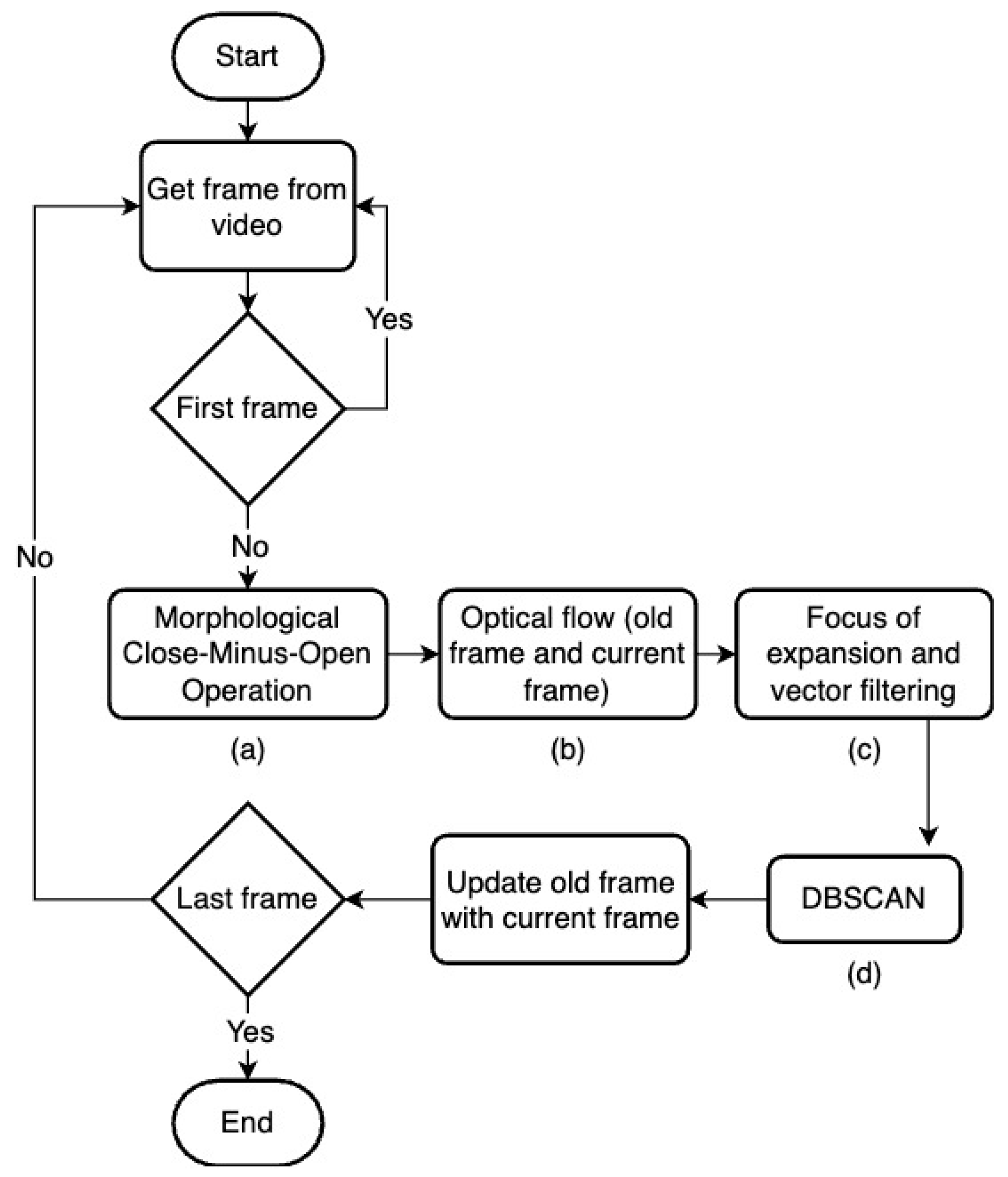
Figure 2.
Schematic views of the three airprox scenarios.
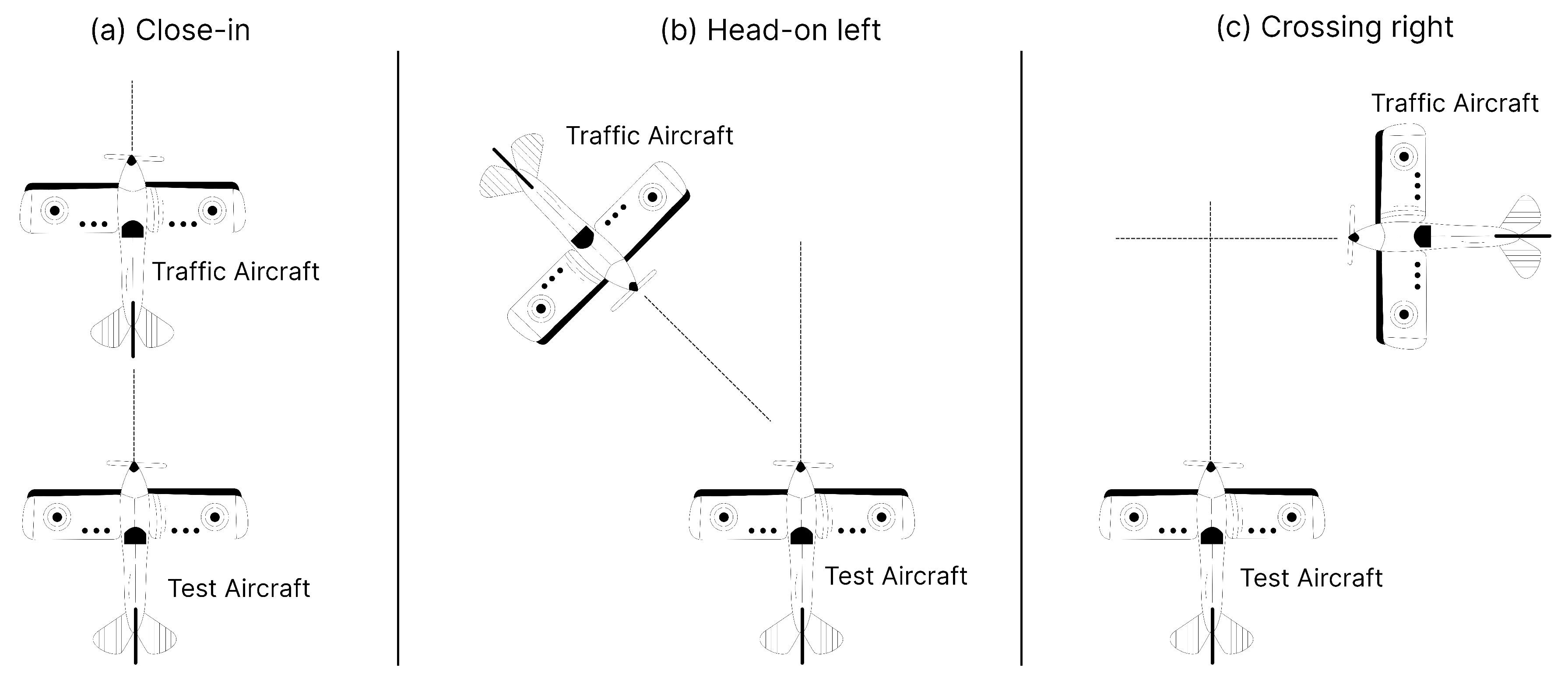
Figure 3.
Close-in scenario snapshots.
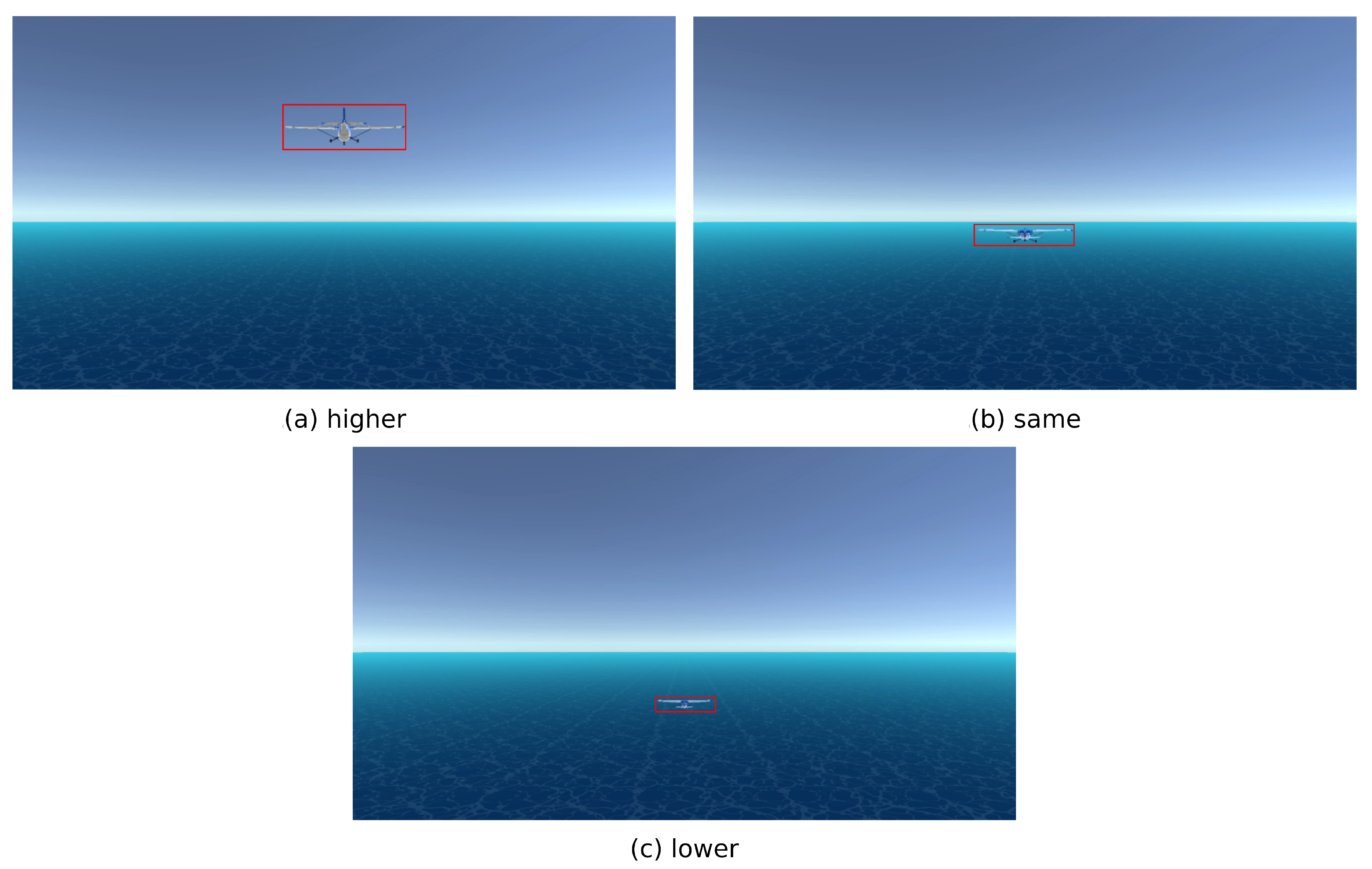
Figure 4.
Head-on scenario snapshots.
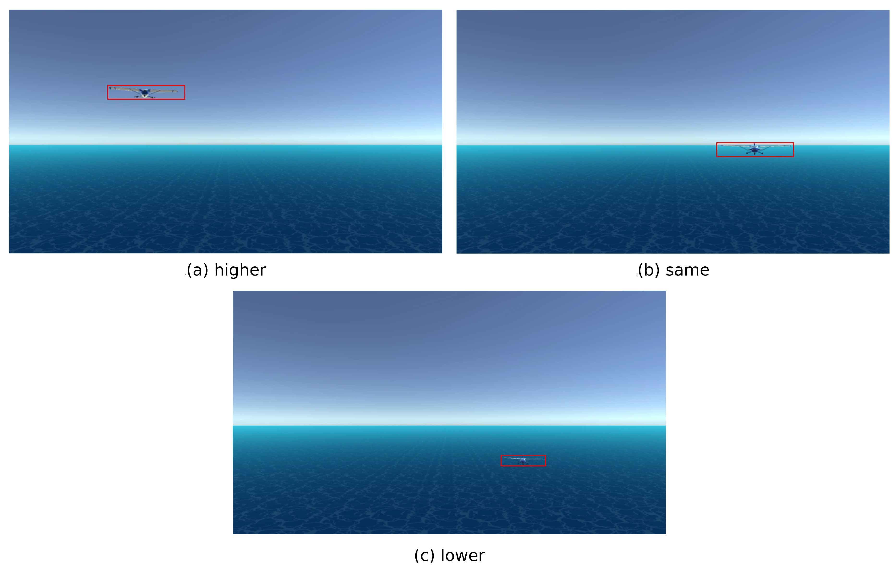
Figure 5.
Crossing scenario snapshots.
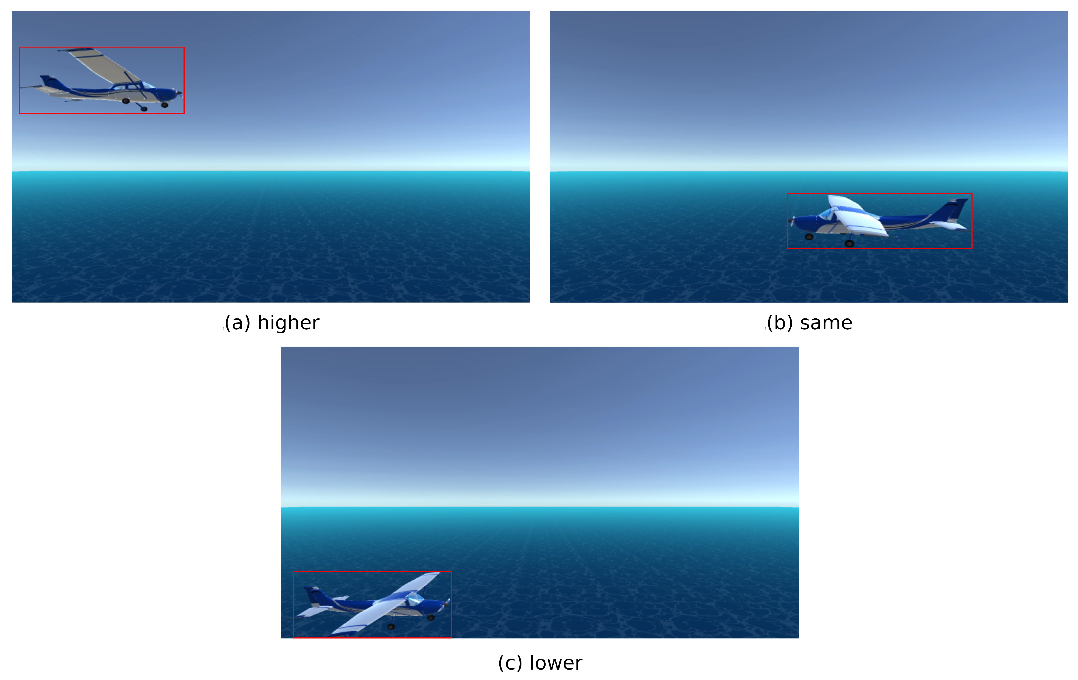
Figure 6.
Cessna 172s - model.
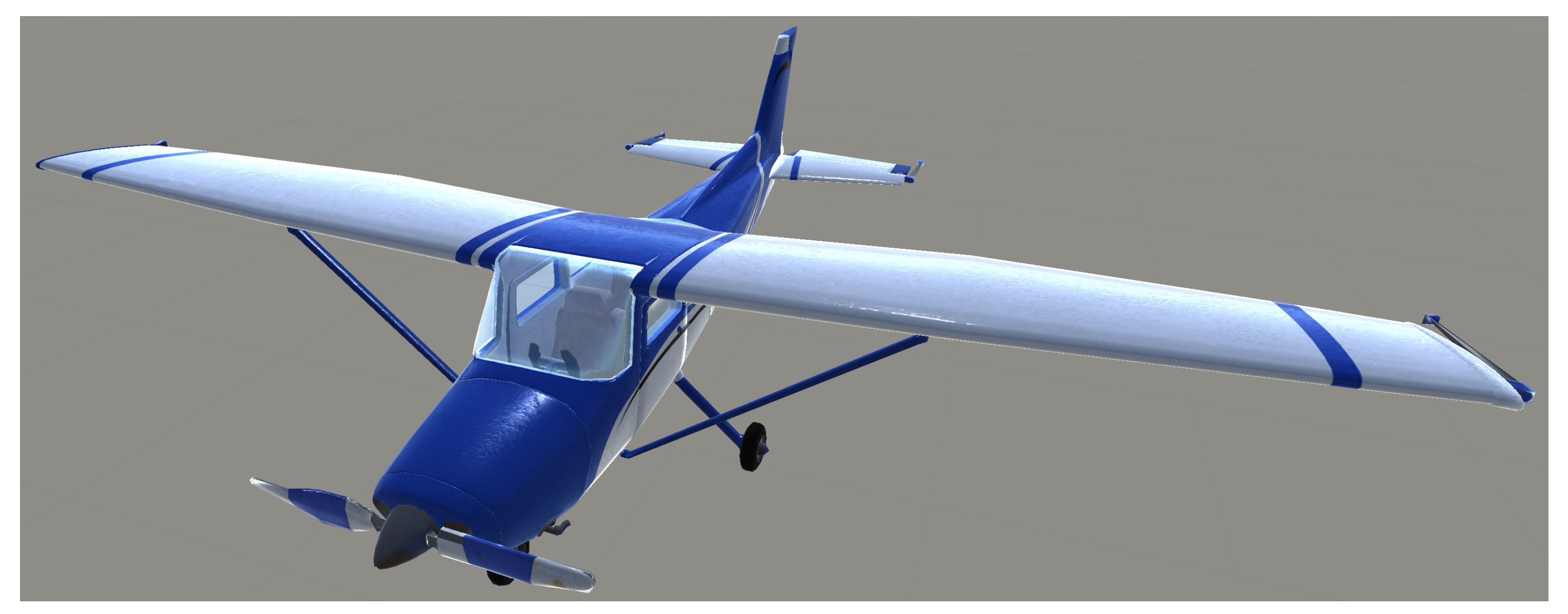
Figure 7.
Close-in time remaining after detection using boxplots.
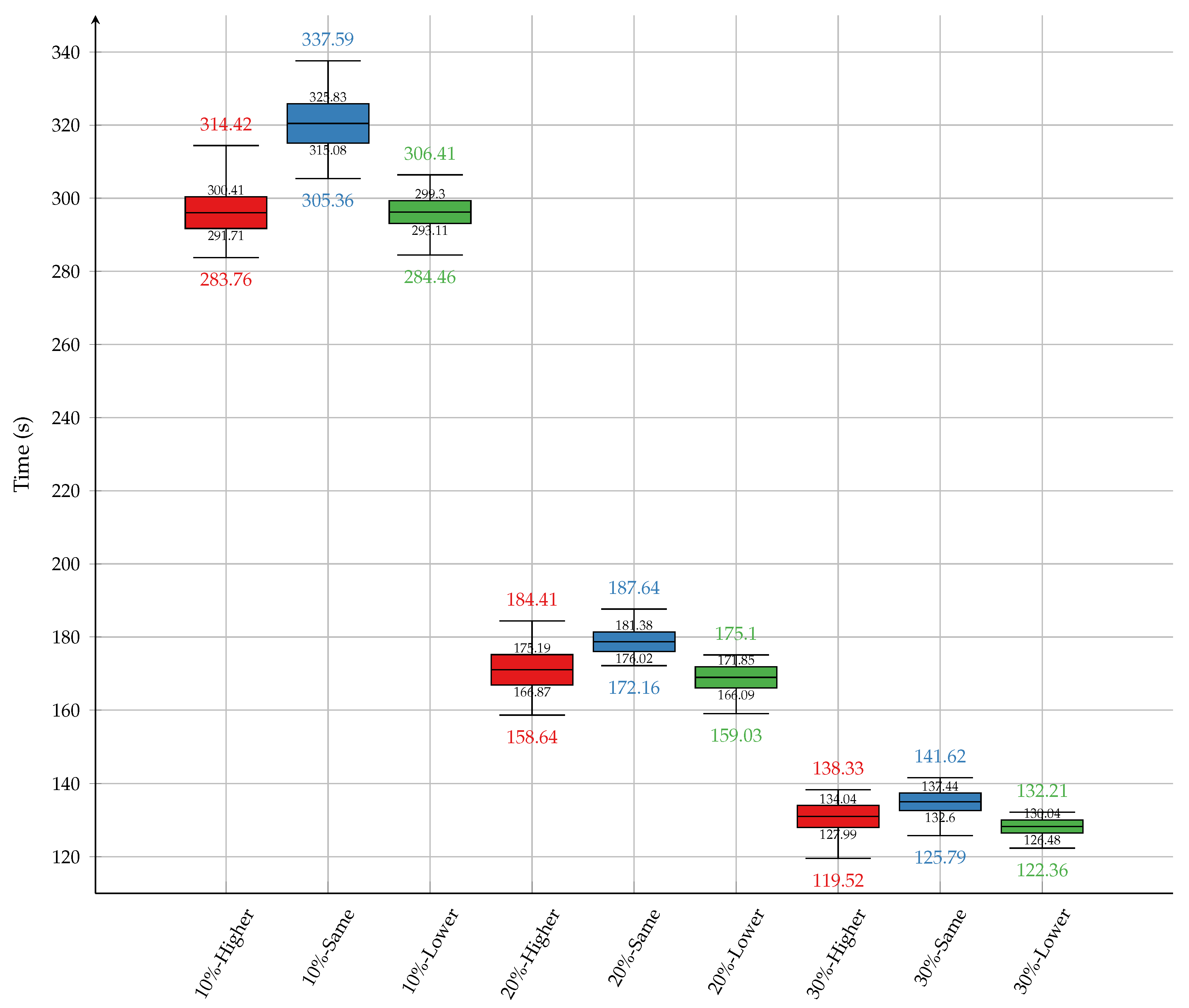
Figure 8.
Close-in - Detection distance, grouped by speed difference.
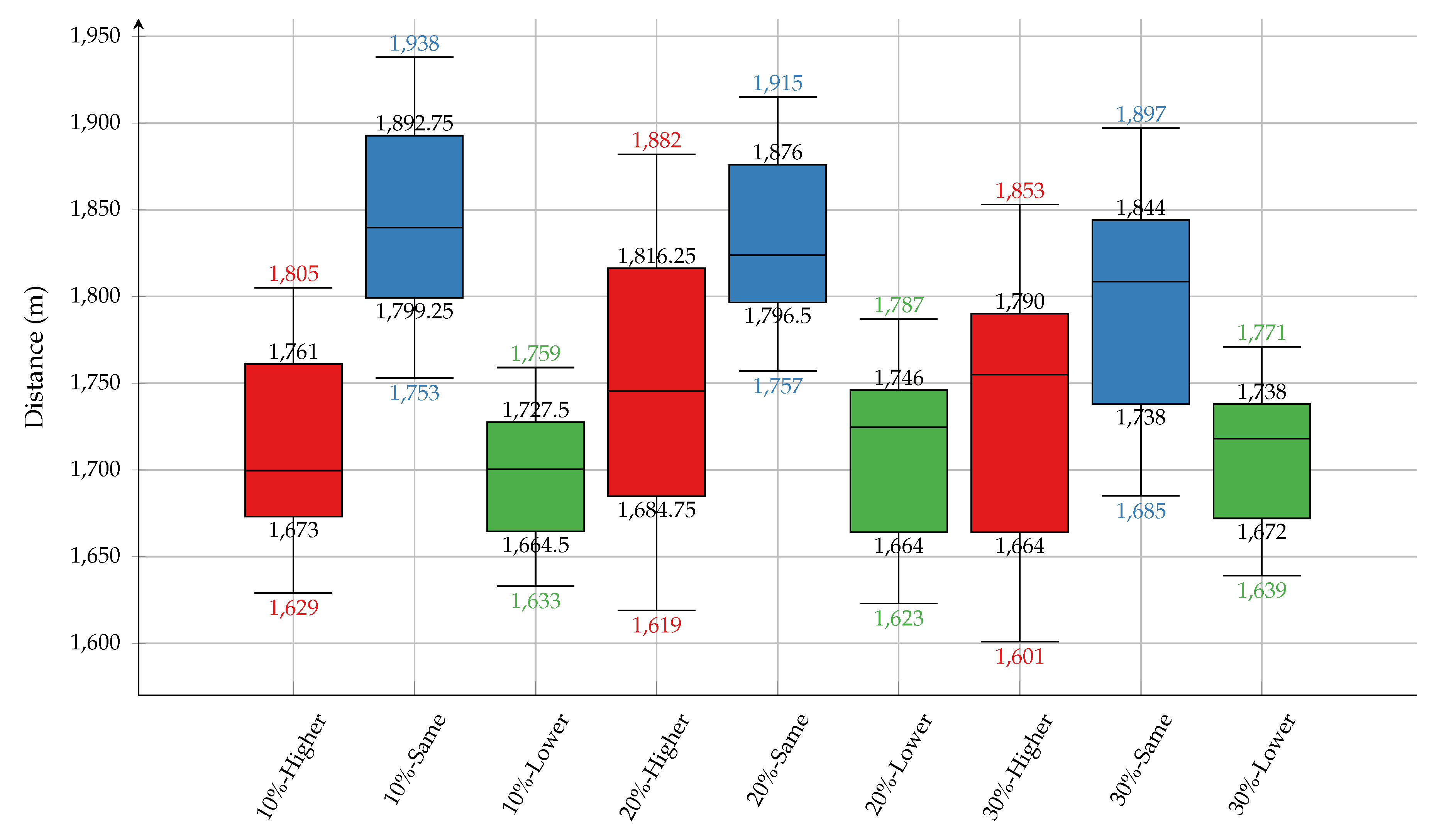
Figure 9.
Head-on - Time remaining after detection, grouped by approach side.
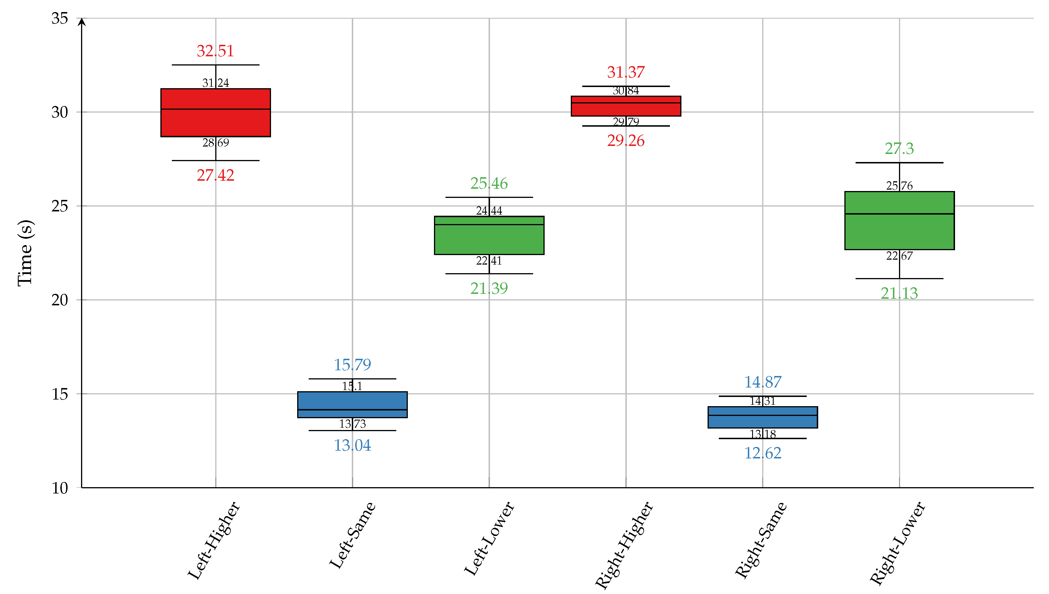
Figure 10.
Head-on - Detection distance, grouped by approach side.
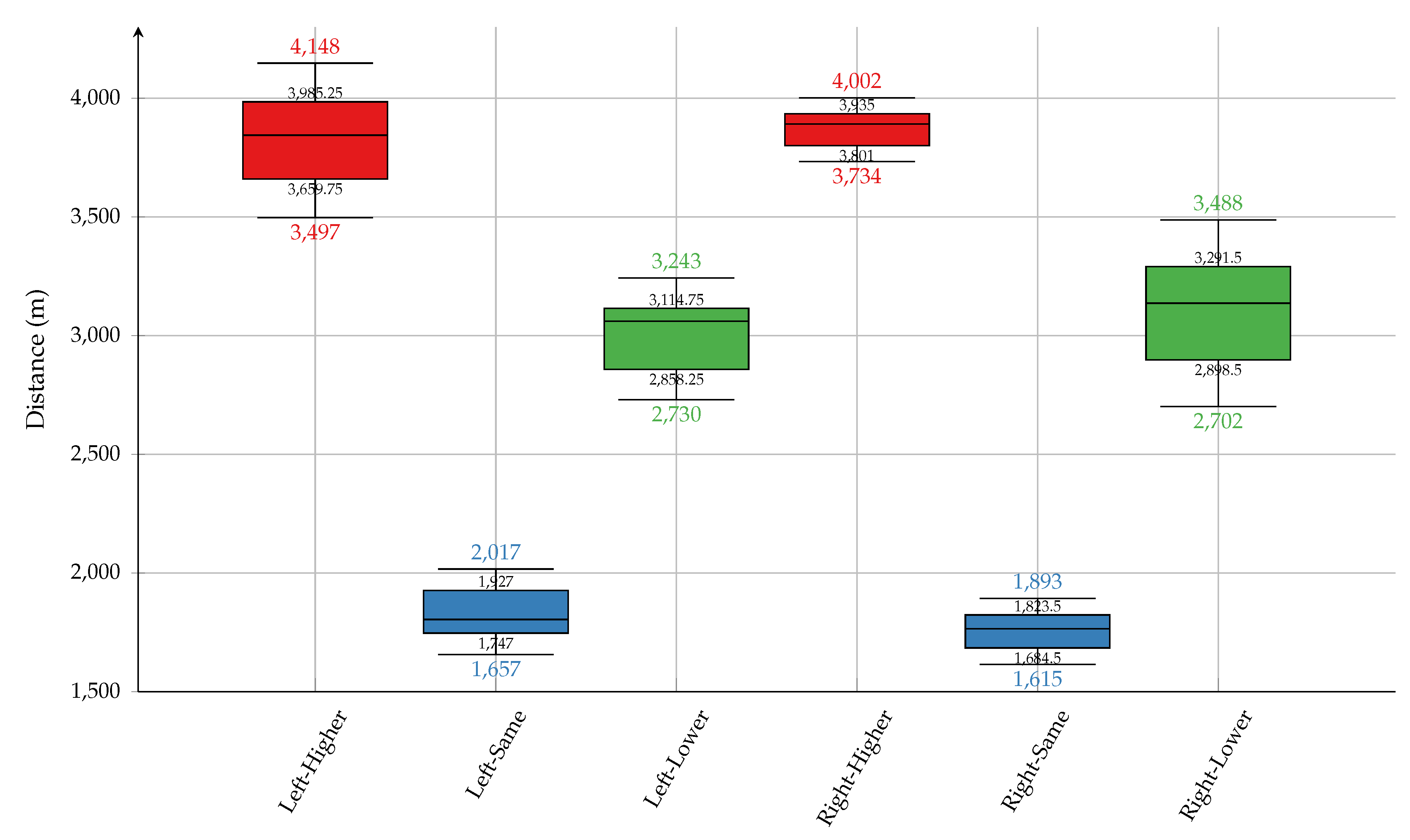
Figure 11.
Crossing - Time remaining after detection, grouped by approach side.
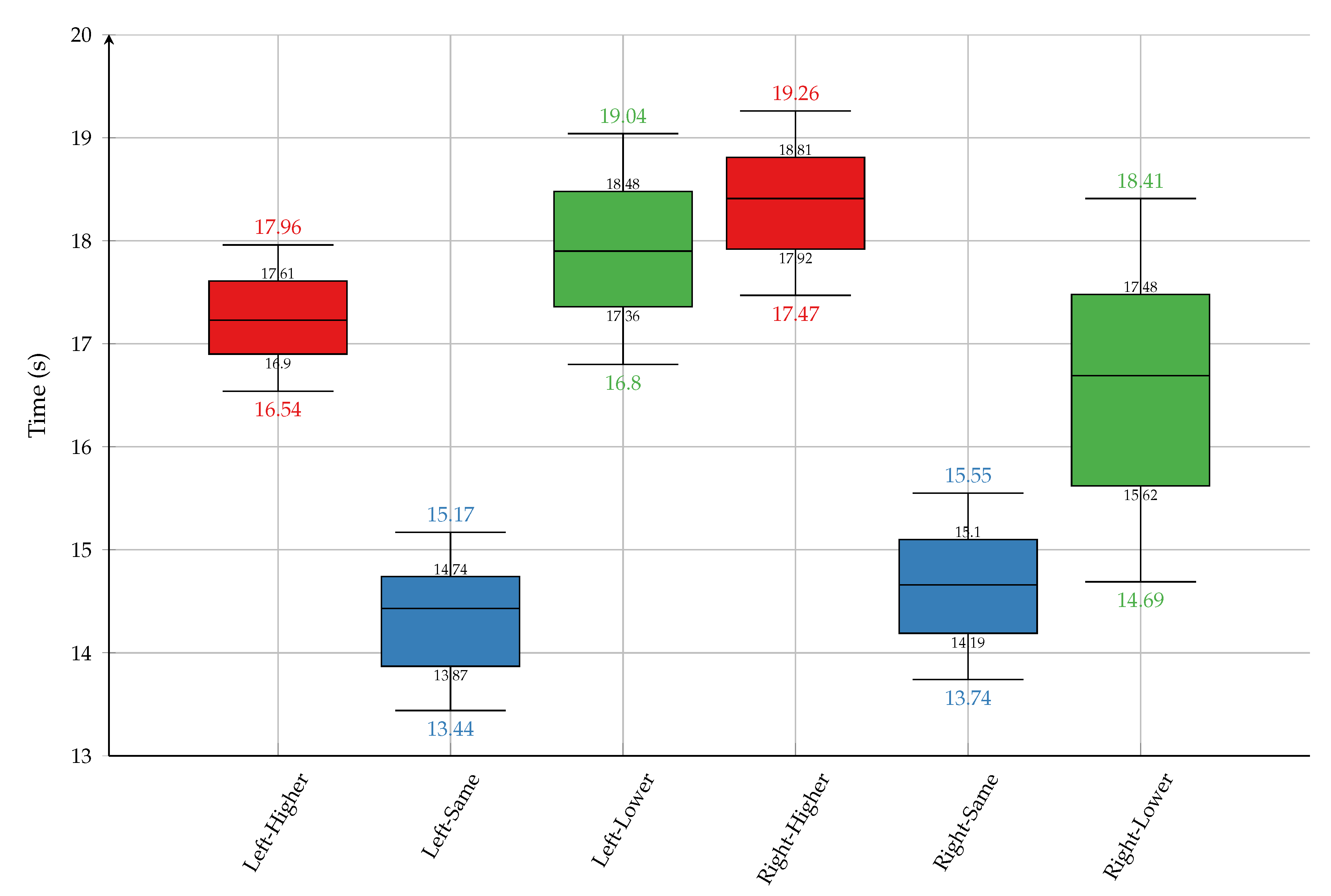
Figure 12.
Crossing - Detection distance, grouped by approach side.
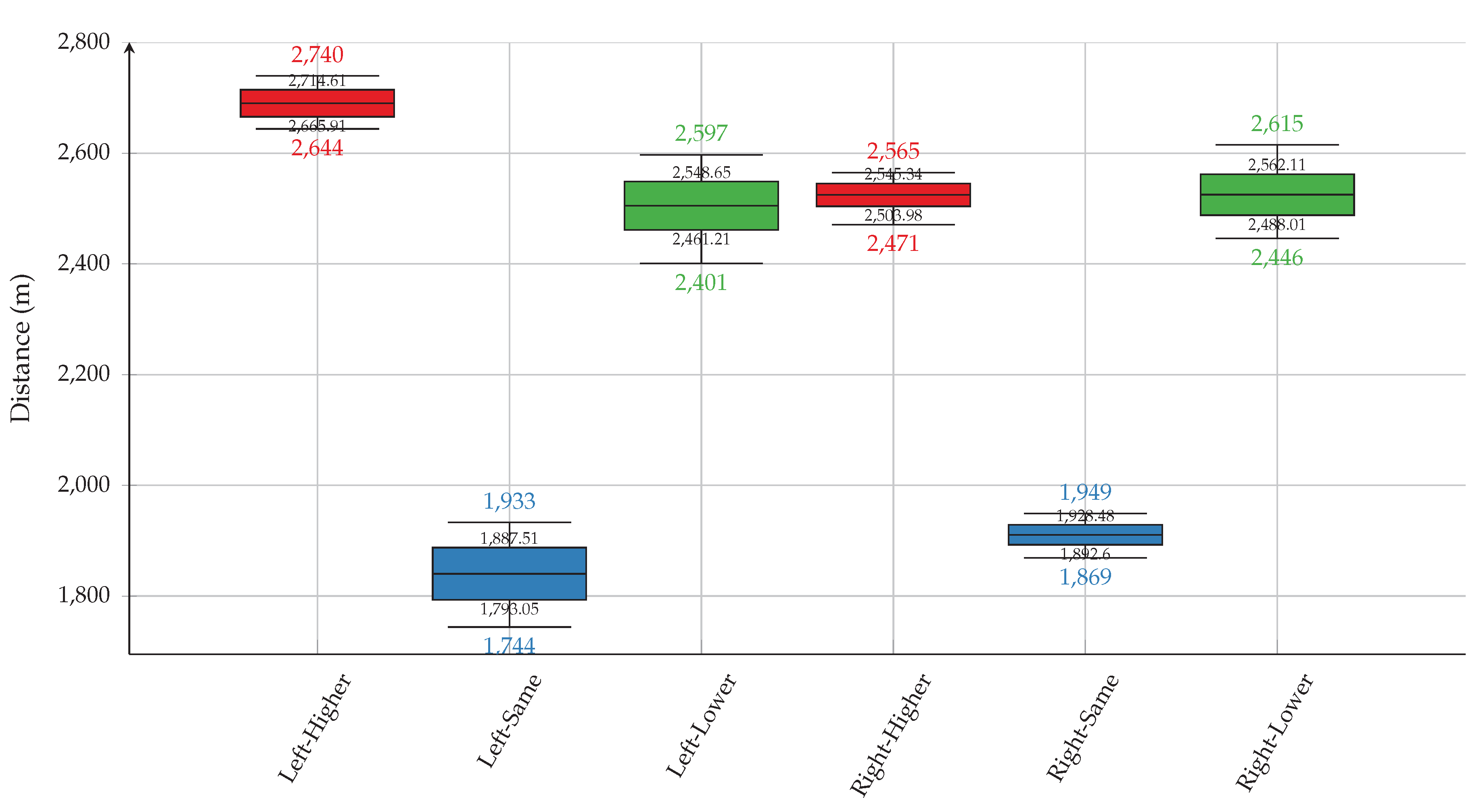

Table 1.
Close-in - Time remaining after detection (in seconds).
| Speed decrease | Obstacle altitude | Minimum | Maximum | Average | Range | Standard deviation |
|---|---|---|---|---|---|---|
| 10% | higher | 283.76 | 314.42 | 296.06 | 30.66 | 8.71 |
| same | 305.36 | 337.59 | 320.45 | 32.23 | 10.75 | |
| lower | 284.46 | 306.41 | 296.20 | 21.95 | 6.19 | |
| 20% | higher | 158.64 | 184.41 | 171.03 | 25.77 | 8.32 |
| same | 172.16 | 187.64 | 178.70 | 15.48 | 5.36 | |
| lower | 159.03 | 175.10 | 168.97 | 16.07 | 5.76 | |
| 30% | higher | 119.52 | 138.33 | 131.01 | 18.81 | 6.05 |
| same | 125.79 | 141.62 | 135.02 | 15.83 | 4.84 | |
| lower | 122.36 | 132.21 | 128.26 | 9.85 | 3.56 |
Table 2.
Close-in - Detection distance (in meters).
| Speed decrease | Obstacle altitude | Minimum | Maximum | Average | Range | Standard deviation |
|---|---|---|---|---|---|---|
| 10% | higher | 1629.00 | 1805.00 | 1699.60 | 176.00 | 49.98 |
| same | 1753.00 | 1938.00 | 1839.60 | 185.00 | 61.72 | |
| lower | 1633.00 | 1759.00 | 1700.40 | 126.00 | 35.50 | |
| 20% | higher | 1619.00 | 1882.00 | 1745.50 | 263.00 | 84.92 |
| same | 1757.00 | 1915.00 | 1823.80 | 158.00 | 54.70 | |
| lower | 1623.00 | 1787.00 | 1724.50 | 164.00 | 58.78 | |
| 30% | higher | 1601.00 | 1853.00 | 1754.90 | 252.00 | 81.06 |
| same | 1685.00 | 1897.00 | 1808.60 | 212.00 | 64.87 | |
| lower | 1639.00 | 1771.00 | 1718.00 | 132.00 | 47.67 |
Table 3.
Head-on - Time remaining after detection (in seconds).
| Airprox side | Obstacle altitude | Minimum | Maximum | Average | Range | Standard deviation |
|---|---|---|---|---|---|---|
| Left | higher | 27.42 | 32.51 | 30.15 | 5.09 | 1.37 |
| same | 13.04 | 15.79 | 14.15 | 2.75 | 0.84 | |
| lower | 21.39 | 25.46 | 24.00 | 4.07 | 1.47 | |
| Right | higher | 29.26 | 31.37 | 30.49 | 2.11 | 0.73 |
| same | 12.62 | 14.87 | 13.85 | 2.25 | 0.71 | |
| lower | 21.13 | 27.30 | 24.58 | 6.17 | 2.21 |
Table 4.
Head-on - Detection distance (in meters).
| Airprox side | Obstacle altitude | Minimum | Maximum | Average | Range | Standard deviation |
|---|---|---|---|---|---|---|
| Left | higher | 3497.00 | 4148.00 | 3844.60 | 651.00 | 175.23 |
| same | 1657.00 | 2017.00 | 1804.70 | 360.00 | 107.21 | |
| lower | 2730.00 | 3243.00 | 3060.50 | 513.00 | 187.69 | |
| Right | higher | 3734.00 | 4002.00 | 3891.5 | 268.00 | 93.35 |
| same | 1615.00 | 1893.00 | 1764.90 | 278.00 | 89.05 | |
| lower | 2702.00 | 3488.00 | 3136.80 | 786.00 | 280.88 |
Table 5.
Crossing - Time remaining after detection (in seconds).
| Airprox side | Obstacle altitude | Minimum | Maximum | Average | Range | Standard deviation |
|---|---|---|---|---|---|---|
| Left | higher | 16.54 | 17.96 | 17.23 | 1.42 | 0.54 |
| same | 13.44 | 15.17 | 14.43 | 1.73 | 0.47 | |
| lower | 16.80 | 19.04 | 17.90 | 2.24 | 0.65 | |
| Right | higher | 17.47 | 19.26 | 18.41 | 1.79 | 0.71 |
| same | 13.74 | 15.55 | 14.66 | 1.81 | 0.71 | |
| lower | 14.69 | 18.41 | 16.69 | 3.72 | 1.24 |
Table 6.
Crossing - Detection distance (in meters).
| Airprox side | Obstacle altitude | Minimum | Maximum | Average | Range | Standard deviation |
|---|---|---|---|---|---|---|
| Left | higher | 2644.00 | 2740.00 | 2690.26 | 96.03 | 36.06 |
| same | 1744.00 | 1933.00 | 1840.28 | 188.13 | 69.97 | |
| lower | 2401.00 | 2597.00 | 2504.93 | 196.01 | 64.77 | |
| Right | higher | 2471.00 | 2565.00 | 2524.66 | 94.22 | 30.62 |
| same | 1869.00 | 1949.00 | 1910.54 | 80.28 | 26.57 | |
| lower | 2446.00 | 2615.00 | 2525.06 | 168.95 | 54.81 |
Disclaimer/Publisher’s Note: The statements, opinions and data contained in all publications are solely those of the individual author(s) and contributor(s) and not of MDPI and/or the editor(s). MDPI and/or the editor(s) disclaim responsibility for any injury to people or property resulting from any ideas, methods, instructions or products referred to in the content. |
© 2026 by the authors. Licensee MDPI, Basel, Switzerland. This article is an open access article distributed under the terms and conditions of the Creative Commons Attribution (CC BY) license.
Copyright: This open access article is published under a Creative Commons CC BY 4.0 license, which permit the free download, distribution, and reuse, provided that the author and preprint are cited in any reuse.


