Vulnerability in Bank-Asset Bipartite Network System: Evidence from the Chinese Banking Sector

1. Introduction

Since the 2008 global financial crisis, the stability of the banking system has attracted mounting attention. As integration between banks’ asset and liability markets deepens, the increasing segmentation and complexity of financial markets have created additional channels for financial risk transmission, which could readily trigger systemic financial risks and amplify the financial system’s vulnerability [1,2]. The various interactions between financial institutions can be conceptualized as a network, and a substantial body of research has employed network theory to identify financial linkages. Therefore, interconnected linkages in financial network can be applied to explore and monitor potential risk contagion channels, thereby characterizing systemic risk and financial stability [3,4,5,6,7].

Financial activities such as interbank lending and bond repurchases establish direct asset-liability linkages among institutions, forming a direct interbank network [8,9]. Amount of studies on interbank networks in different markets have systematically elaborated their structural characteristics, such as small-world properties, scale-free features, and core-periphery structures, and their significant impacts on risk diffusion [10,11]. While the interbank lending market compensates for banks’ temporary liquidity shortages, it also provides a channel for risk accumulation and contagion. Extensive research has shown that the correlation between network structure and risk contagion is not linear, with interbank networks exhibiting “robust-yet-fragile” characteristic [12,13,14,15].

Beyond direct financial linkages, scholarly attention has also centered on systemic risk transmission via indirect connections, most notably through common asset holdings across financial institutions. Scholars have extensively examined the influence of several key factors, including asset prices, market sentiment, trading strategies, and regulatory frameworks—on the mechanisms of risk contagion. Duarte and Eisenbach [16] developed a “vulnerability index” for banks’ asset fire sales to examine systemic vulnerability arising from contagion spillovers. Huang et al. [17] and Levy-Carciente et al. [18] analyzed the cascading effects of systemic risk contagion in the U.S. and Venezuelan banking systems, respectively, using bank-asset network models. Caccioli et al. [19] built a bipartite bank-asset network to investigate system stability under fire sales of overlapping portfolios, and Caccioli et al. [20] later extended this by developing a network model incorporating both interbank transactions and common asset fire sales to empirically assess systemic risks across these two contagion channels. Greenwood et al. [21] integrated leverage targets into the fire sale mechanism, quantifying deleveraging-induced risk spillovers among European banks during the 2010-2011 sovereign debt crisis. Additionally, Coen et al. [22] modeled the shock amplification process by accounting for leverage-constrained banks, risk-weighted capital, and liquidity regulations. Meanwhile, the quantification of systemic risk in non-banking financial sectors, such as investment funds, insurance, and currency market, has also gained scholars’ attention through indirect contagion channels [23,24]. For example, Douglas et al. [25] focused on the impact of Solvency II regulation on the distressed portfolio adjustments of UK life insurers. Barucca et al. [26] studied common security holdings across UK banks, focusing on the network structure of overlapping portfolios. Building on this work, Caccioli et al. [27] extended the analysis to investigate how overlapping portfolio network structures affect shock propagation using more granular data.

In practice, the disclosure of asset positions by financial institutions is often insufficient. To overcome this limitation, several methods have been developed to reconstruct networks from available data. These methods vary in their emphasis on different network features. Some seek to minimize the exposures of individual links, while others focus on replicating aggregate network outputs. Techniques such as maximum entropy estimation, minimum density estimation, and network configuration models have been widely applied [28]. However, the standard maximum entropy method, which assumes full node connectivity, often conflicts with real-world linkages and can severely underestimate risk contagion effects. Squartini et al. [29] proposed a constrained entropy maximization method for bipartite networks, showing it outperforms traditional CAPM and maximum entropy CAPM in characterizing topological structures and estimating fire sale risks. Di Gangi et al. [30] used cross-entropy constraint minimization to assess the systemic importance of banking systems and individual institutions using only bank size and asset investment data. Gandy and Veraart [31] developed a tunable network reconstruction model via empirical Bayesian methods to adjust networks to match observed specific expectations. Ramadiah et al. [32] theoretically reconstructed Japan’s bank-firm credit networks using four methods (CM1, CM2, MinDensity, MaxEntropy) and compared the differences in systemic risk levels across these approaches.

Chinese commercial banks play a decisive role in China’s financing market, and the loans issued to the real economy account for over 60% of the social financing scale stock in recent years. Therefore, it is critical to evaluate banking system vulnerability by considering both direct and indirect contagion channels. This article contributes to this field by introducing a network stress model to analyze shock propagation dynamics. Using balance sheet data from Chinese commercial banks between 2016 and 2022, we employ Exponential Random Graph Models to reconstruct the bipartite network of banks’ asset allocation. We then analyze the network’s topological characteristics and measure its similarity to real structures. Subsequently, a novel framework for measuring aggregate network vulnerability is employed. This framework incorporates factors such as bank size, initial shocks, connectedness, leverage, and asset fire sales to identify financial contagion effects. Through simulation, this paper explores the dynamic evolution of risk contagion, as well as the vulnerability of the banking network system. The aim is to provide technical and methodological support for banks to enhance their asset allocation capabilities and for financial regulatory authorities to implement targeted risk management policies.

The paper proceeds as follows. Section 2 outlines the network reconstruction methodology and presents the vulnerability measurement model. Section 3 describes the data and validates the reconstructed network’s similarity to the actual system. Section 4 simulates aggregate network vulnerabilities across different shock scenarios. Section 5 concludes.

2. Methodology

Based on bank balance sheets, the linkages between commercial banks and their held assets can be conceptualized as a bipartite network$\mathrm{G}(\mathrm{X},\mathrm{Y},\mathrm{E})$. This network consists of two disjoint, non-empty vertex sets: a set$\text{{}\mathrm{X}\text{}}$ representing bank nodes and a set$\text{{}\mathrm{Y}\text{}}$ denoting asset nodes. The set of edges$\text{{}\mathrm{E}\text{}}$ connects banks to the assets they hold. This structure is represented by a matrix $\mathrm{A}$of dimensions$\mathrm{N}*\mathrm{M}$, capturing$\mathrm{N}$ banks and$\mathrm{M}$ asset types. Each element${\mathrm{A}}_{\mathrm{i},\mathrm{j}}$within the matrix denotes the value of asset type$\mathrm{j}$held by bank$\mathrm{i}$. The total value of assets in the network is${\sum }_{\mathrm{i}=1}^{\mathrm{N}}{\sum }_{\mathrm{j}=1}^{\mathrm{M}}{\mathrm{A}}_{\mathrm{i},\mathrm{j}}$; the total value of assets held by a single bank $\mathrm{i}$ is${\sum }_{\mathrm{j}=1}^{\mathrm{M}}{\mathrm{A}}_{\mathrm{i},\mathrm{j}}$; and the total value of a specific asset type$\mathrm{j}$ held across the entire network is${\sum }_{\mathrm{i}=1}^{\mathrm{N}}{\mathrm{A}}_{\mathrm{i},\mathrm{j}}$.

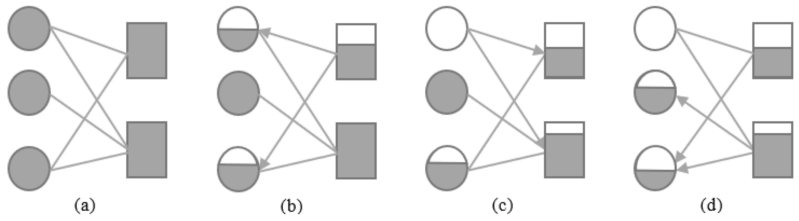
2.1. Network reconstruction

Using the accessible data on banks’ strength sequence$\left\{{\mathrm{S}}_{\mathrm{i}}\right\}$, assets’ strength sequence$\left\{{\mathrm{S}}_{\mathrm{j}}\right\}$, and the total number of bank-asset links$\mathrm{L}$, we reconstruct the bipartite network of banks’ asset allocation according to the method outlined by Squartini et al. [29].

(1)First step: Using Exponential Random Graph Models, we generate an ensemble, denoted Ω, of randomized bipartite networks. These networks are constrained to obtain the same number of $\mathrm{N}\text{×}\mathrm{M}$nodes as the observed system. From this ensemble, a representative network${\mathrm{G}}_0$ can be extracted to infer the most probable bank-asset holding relationships. For any potential link between bank $\mathrm{i}$and asset$\mathrm{j}$, the probability${\mathrm{p}}_{\mathrm{ij}}\text{≡}{⟨{\stackrel{\mathrm{~}}{\mathrm{a}}}_{\mathrm{ij}}⟩}_{\mathsf{\Omega }}={\displaystyle \frac{{\mathrm{x}}_{\mathrm{i}}{\mathrm{y}}_{\mathrm{j}}}{1+{\mathrm{x}}_{\mathrm{i}}{\mathrm{y}}_{\mathrm{j}}}}$is calculated over the entire ensemble Ω. We assume that the observed strength of each node (the total value of assets for a bank or the total value held for an asset) serves as a fitness measure. The strength value${\left\{{\mathrm{S}}_{\mathrm{i}}\right\}}_{\mathrm{i}\text{∈}\mathrm{N}}$and${\left\{{\mathrm{S}}_{\mathrm{j}}\right\}}_{\mathrm{j}\text{∈}\mathrm{M}}$are modeled as being linearly proportional to the Lagrange multipliers, ${\mathrm{x}}_{\mathrm{i}}\text{≡}\sqrt{{\mathrm{z}}_{\mathrm{i}}}{\mathrm{S}}_{\mathrm{i}},\text{∀}\mathrm{i}$ and${\mathrm{y}}_{\mathrm{j}}\text{≡}\sqrt{{\mathrm{z}}_{\mathrm{j}}}{\mathrm{S}}_{\mathrm{j}},\text{∀}\mathrm{j}$, which are induced by constraining the expected nodes’ degree in the maximum entropy formulation of the ERGMs.

(2)Second step: By equating the ensemble Ω average of the total number of edges with the actual total number $\mathrm{L}$of edges of${\mathrm{G}}_0$: ${⟨\mathrm{L}⟩}_{\mathsf{\Omega }}={\sum }_{\mathrm{i}}{\sum }_{\mathrm{j}}{\displaystyle \frac{\mathrm{z}{\mathrm{S}}_{\mathrm{i}}{\mathrm{S}}_{\mathrm{j}}}{1+\mathrm{z}{\mathrm{S}}_{\mathrm{i}}{\mathrm{S}}_{\mathrm{j}}}}=\mathrm{L}\left({\mathrm{G}}_0\right)$, where we have already defined$\mathrm{z}=\sqrt{{\mathrm{z}}_{\mathrm{i}}{\mathrm{z}}_{\mathrm{j}}}$. Then, $\mathrm{z}$ is the single positive solution of the equation, which can be used to estimate the linking probabilities ${\mathrm{p}}_{\mathrm{ij}}={⟨{\stackrel{\mathrm{~}}{\mathrm{a}}}_{\mathrm{ij}}⟩}_{\mathsf{\Omega }}={\displaystyle \frac{\mathrm{z}{\mathrm{S}}_{\mathrm{i}}{\mathrm{S}}_{\mathrm{j}}}{1+\mathrm{z}{\mathrm{S}}_{\mathrm{i}}{\mathrm{S}}_{\mathrm{j}}}},\text{∀}(\mathrm{i},\mathrm{j})$.

(3)Third step: Given the network topology determined by nontrivial linkage probabilities, weights of links are thus determined as:${\stackrel{\mathrm{~}}{\mathrm{w}}}_{\mathrm{ij}}={\displaystyle \frac{{\mathrm{S}}_{\mathrm{i}}{\mathrm{S}}_{\mathrm{j}}}{\mathrm{W}{\mathrm{p}}_{\mathrm{ij}}}}{\stackrel{\mathrm{~}}{\mathrm{a}}}_{\mathrm{ij}}=({\mathrm{z}}^{-1}+{\mathrm{S}}_{\mathrm{i}}{\mathrm{S}}_{\mathrm{j}}){\displaystyle \frac{{\stackrel{\mathrm{~}}{\mathrm{a}}}_{\mathrm{ij}}}{\mathrm{W}}}$, where $\mathrm{W}$ is expressed as the total amount of assets. To sum up, the set of linking probabilities and link strength determine the ensemble Ω, so that the value of asset holding quantity$\mathrm{X}$ in${\mathrm{G}}_0$ could be estimated as its ensemble average${⟨\mathrm{X}⟩}_{\mathsf{\Omega }}$.

2.2. Network reconstruction

Following the approach proposed by Huang et al. [17], we measure systemic vulnerability by the cumulative losses from financial contagion triggered by exogenous shocks to specific asset classes. Then, we first systematically deconstruct the mechanisms of risk contagion within bank-asset holding networks (as illustrated in Figure 1) and subsequently construct a corresponding model to simulate its evolution.

Figure 1(a) illustrates the distribution of assets held across banks. Given the overlapping nature of bank asset portfolios, an exogenous shock to a specific asset class (Figure 1(b)) transmits losses to all banks holding that asset. If these losses render a bank insolvent (Figure 1(c)), it is forced to engage in fire sales to meet its obligations. The surge in selling pressure drives down the market price of the asset. This devaluation forces other banks holding the same asset to mark down its value, eroding their net worth and potentially triggering further insolvency. This dynamic initiates a negative feedback loop of fire sales and price declines, propagating contagion throughout the network (Figure 1(d)).

For a bipartite network consisting of$\mathrm{N}$ banks and$\mathrm{M}$ assets, we set bank $\mathrm{i}\text{'}\mathrm{s}$ liabilities as${\mathrm{L}}_{\mathrm{i}}$, equity as${\mathrm{E}}_{\mathrm{i}}$, and total assets as${\mathrm{A}}_{\mathrm{i}}={\sum }_{\mathrm{j}=1}^{\mathrm{M}}{\mathrm{A}}_{\mathrm{ij}}={\mathrm{E}}_{\mathrm{i}}+{\mathrm{L}}_{\mathrm{i}}$. Let${\mathrm{A}}_{\mathrm{i},\mathrm{j},\mathrm{T}}$ and ${\mathrm{K}}_{\mathrm{i},\mathrm{j},\mathrm{T}}$denote the value of asset held by bank$\mathrm{i}$ and the leverage ratios with${\mathrm{K}}_{\mathrm{i},\mathrm{j},\mathrm{T}}={\displaystyle \frac{{\mathrm{L}}_{\mathrm{ijT}}}{{\mathrm{E}}_{\mathrm{ijt}}}}$ at time step$\mathrm{T}$. Meanwhile, let${\mathrm{M}}_{\text{{}\mathrm{N}*\mathrm{M}\text{}}}$denote the matrix of portfolio weights, where each element${0\text{≤}\mathrm{M}}_{\mathrm{i},\mathrm{j}}\text{≤}1$ is the market-value-weighted share of asset$\mathrm{j}$ in bank$\mathrm{i}\text{'}\mathrm{s}$ portfolio, and${{\text{∑}}_{\mathrm{j}}\mathrm{M}}_{\mathrm{i},\mathrm{j}}=1$. We introduce an parameter $-\mathrm{q}$($\mathrm{q}$∈[0, 1]) to characterize the negative impact level from initial shocks, and an coefficient matrix-$\mathsf{\xi }$(${\mathsf{\xi }}_{\mathrm{i}}$∈[0, 1]) to measure the price impact from asset sales. Therefore, aggregate vulnerability of the bank-asset allocation network can be calculated through systemic risk contagion process as follows.

(1)Initial shock. Assuming that any asset$\mathrm{j}$ held by banks be subject to an external shock, the net value of asset after the shock can be expressed as${\mathrm{A}}_{\mathrm{j},1}=\mathrm{q}{\mathrm{A}}_{\mathrm{j},0}$, where$\mathrm{q}$ represents the proportion of residual value of the asset ${\mathrm{m}}^{\text{'}}$ after the shock. Moreover, the value of the same type of asset decreases proportionally, expressed as${\mathrm{B}}_{\mathrm{i},\mathrm{j},1}=\mathrm{q}{\mathrm{B}}_{\mathrm{i},\mathrm{j},0}={\mathrm{B}}_{\mathrm{i},\mathrm{j},0}{\displaystyle \frac{{\mathrm{A}}_{\mathrm{j},1}}{{\mathrm{A}}_{\mathrm{j},0}}}$.

(2)Leverage target. After the initial shock, banks should maintain a fixed leverage target on a mark-to-market basis in line with the empirical evidence [33]. If${\mathrm{B}}_{\mathrm{i}}\text{＞}{\mathrm{L}}_{\mathrm{i}}$, and some banks face higher leverage ratios due to asset depreciation, they have to sell assets to deleverage. If${\mathrm{B}}_{\mathrm{i}}\text{≤}{\mathrm{L}}_{\mathrm{i}}$, banks become insolvent and undergo liquidation. In terms of banks selling assets to target leverage, each bank asset can be modified as${\mathrm{A}}_{\mathrm{i},\mathrm{T}+1}={\mathrm{A}}_{\mathrm{i},\mathrm{T}}-\mathsf{\alpha }({\mathsf{\lambda }}_{\mathrm{i},\mathrm{j},\mathrm{T}}{\mathrm{B}}_{\mathrm{i},\mathrm{j},\mathrm{T}}^{\mathrm{Del}})$, where$\mathsf{\lambda }$ denotes the proportion of asset be sold ($\mathrm{i}\text{∈}{\text{{}\mathrm{Deleverage}\mathrm{Set}\text{}}}_{\mathrm{T}}$). Moreover, we make a simply assumption that banks sell assets in proportion to their actual holdings, so the parameter$\mathsf{\lambda }$ can be expressed as${\mathsf{\lambda }}_{\mathrm{i},\mathrm{j},\mathrm{T}}={\displaystyle \frac{{\mathsf{\omega }}_{\mathrm{i},\mathrm{j},\mathrm{T}}*{\mathrm{DEL}}_{\mathrm{i},\mathrm{T}}}{{\mathrm{B}}_{\mathrm{i},\mathrm{j},\mathrm{T}}^{\mathrm{Del}}}}$. By the way, if some banks become insolvent, they enter bankruptcy liquidation, and all assets are forced to be sold, therefore bank asset should be expressed as${\mathrm{A}}_{\mathrm{i},\mathrm{T}+1}={\mathrm{A}}_{\mathrm{i},\mathrm{T}}-\mathsf{\alpha }{\mathrm{B}}_{\mathrm{i},\mathrm{j},\mathrm{T}}^{\mathrm{Def}}$; while, if some banks fail, asset prices are jointly influenced by both bankruptcy liquidation and asset sales, therefore the bank asset could be expressed as${\mathrm{A}}_{\mathrm{i},\mathrm{T}+1}={\mathrm{A}}_{\mathrm{i},\mathrm{T}}-\mathsf{\alpha }({\mathsf{\lambda }}_{\mathrm{i},\mathrm{j},\mathrm{T}}{\mathrm{B}}_{\mathrm{i},\mathrm{j},\mathrm{T}}^{\mathrm{Del}}+{\mathrm{B}}_{\mathrm{i},\mathrm{j},\mathrm{T}}^{\mathrm{Def}})$, where$\mathsf{\lambda }{\mathrm{B}}_{\mathrm{i},\mathrm{j},\mathrm{T}}^{\mathrm{Del}}$and${\mathrm{B}}_{\mathrm{i},\mathrm{j},\mathrm{T}}^{\mathrm{Def}}$denote asset sales and asset liquidation respectively.

(3)Fire sales effect. Banks’ asset sales trigger price impact, leading to risk contagion within the system and thereby affecting the equity of banks’ asset return, which can be modified as${\mathrm{B}}_{\mathrm{i},\mathrm{j},\mathrm{T}+1}^{\mathrm{Oth}}={\mathrm{B}}_{\mathrm{i},\mathrm{j},\mathrm{T}}^{\mathrm{Oth}}*{\displaystyle \frac{{\mathrm{A}}_{\mathrm{i},\mathrm{T}+1}}{{\mathrm{A}}_{\mathrm{i},\mathrm{T}}}}$. Meanwhile, asset fire-sales also impacts the value of remaining assets held by deleveraging banks, which can be expressed as${\mathrm{B}}_{\mathrm{i},\mathrm{j},\mathrm{T}+1}^{\mathrm{Del}}=(1-{\mathsf{\lambda }}_{\mathrm{i},\mathrm{j},\mathrm{T}}){\mathrm{B}}_{\mathrm{i},\mathrm{m},\mathrm{T}}^{\mathrm{Del}}*{\displaystyle \frac{{\mathrm{A}}_{\mathrm{i},\mathrm{T}+1}}{{\mathrm{A}}_{\mathrm{i},\mathrm{T}}}}$. In this paper, we let the price impact ratios be a diagonal matrix$\mathsf{\xi }$ on a linear impact assumption, meaning that the price impact only affect the same asset. Therefore, matrix$\mathsf{\xi }$ is set to characterize the proportion of assets actively sold by banks so as to update the market value of banks’ assets dynamically. According to the aforementioned risk contagion process, the iteration continues until no further asset sales or liquidations are triggered.

Overall, aggregate vulnerability of the network can be calculated as${\mathrm{AV}=(1}_{\mathrm{N}}^{\text{'}}{\mathrm{A}}_1\mathrm{M}\mathsf{\xi }\mathrm{M}\text{'}\mathrm{K}{\mathrm{A}}_1\mathrm{Mq})/{\mathrm{E}}_0$ through the risk contagion, which does not involve any direct impact and focus only on the spillovers across banks. For example, if all the assets are liquid perfectly, then$\mathrm{AV}=0$. Note that$1_{\mathrm{N}}^{\text{'}}$ is the$1*\mathrm{N}$ vector of ones. Therefore, the direct vulnerability of each bank from initial shock can be generated as${\mathrm{DV}=1}_{\mathrm{N}}^{\text{'}}{\mathrm{A}}_1\mathrm{Mq}$, and the indirect vulnerability on each bank due to risk contagion can be ${\mathrm{IV}=(1}_{\mathrm{N}}^{\text{'}}{\mathrm{A}}_1\mathrm{M}\mathsf{\xi }\mathrm{M}\text{'}\mathrm{K}{\mathrm{A}}_1\mathrm{Mq})/{\mathrm{E}}_{\mathrm{i}\mathrm{j}}$.

3. Data and Network

3.1. Data and network index

This study utilizes data from the China Stock Market & Accounting Research (CSMAR) database. The sample encompasses Chinese commercial banks whose aggregate assets represent the top 95% of the industry’s total from 2016 to 2022. The final sample includes six large state-owned banks, twelve national joint-stock commercial banks, and the most significant city and rural commercial banks (see Appendix A for a complete list). The annual count of banks in the sample is provided in Table 1. The data processing procedure is as follows: (1) Sample Selection: Commercial banks ranking in the top 95% by total assets are selected, while policy banks and foreign banks are excluded. (2) Asset Classification: Based on balance sheet items and bank annual report disclosures, cash and loan sub-assets are expanded into a detailed classification scheme, resulting in 47 distinct asset categories (detailed in Appendix B). (3) Data Imputation: For banks with missing granular asset portfolio data, gaps are filled using publicly available annual report disclosures. Bank nodes with persistently missing data after this process are excluded from the analysis. (4) Data Scaling: For computational convenience, all asset portfolio values are normalized at a ratio of 1,000,000,000:1. Finally, a set of network topology indicators, presented in Table 2, are calculated to characterize the structure of the reconstructed bank-asset network.

3.2. Data and network index

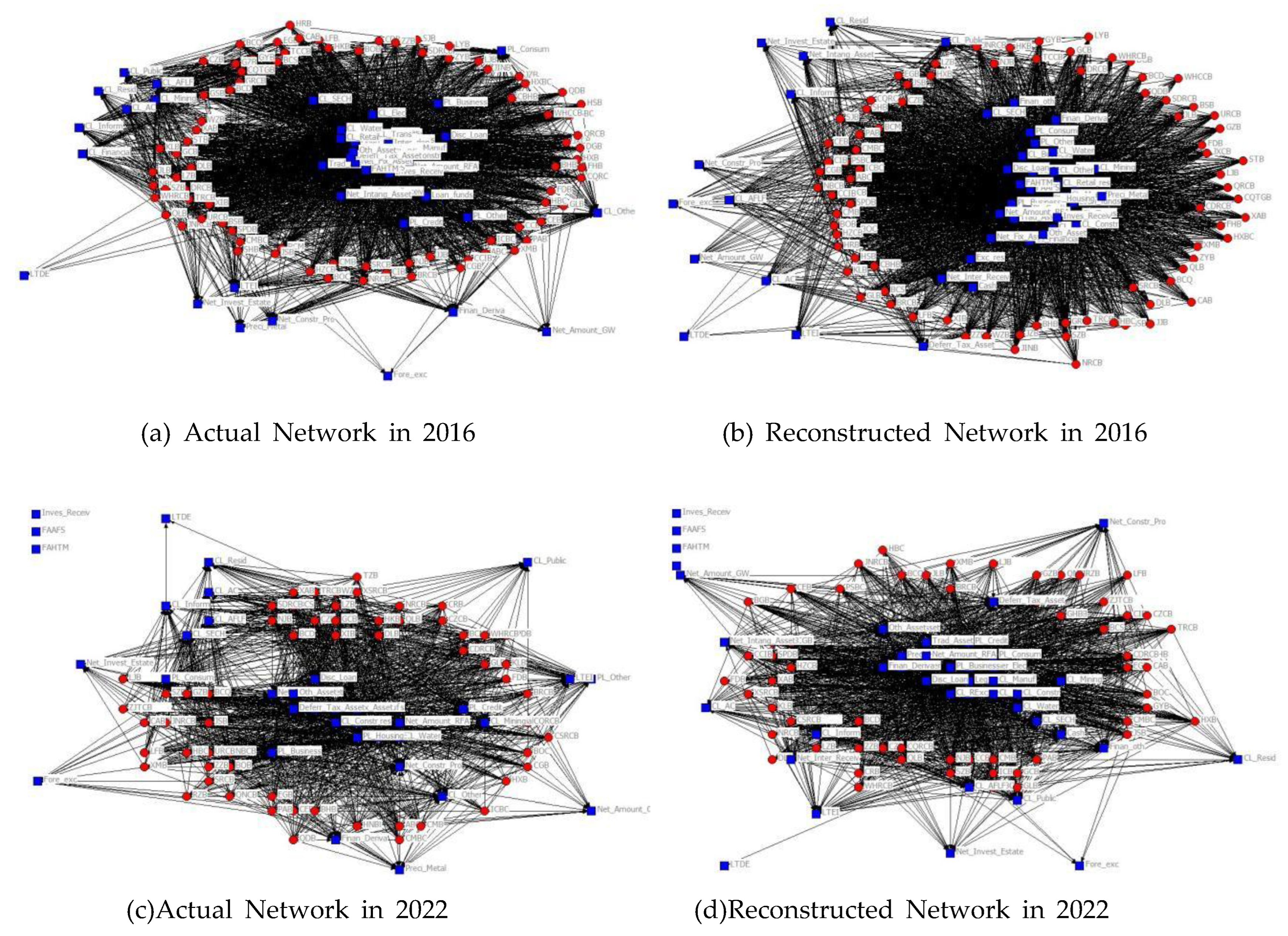
3.2.1. Topology structure

Utilizing available data on bank asset holdings from 2016 to 2022, we construct annual bank-asset bipartite networks to analyze their macro-level topological structures. Figure 2(a) and Figure 2(b) depict the topology of the actual and reconstructed networks for 2016, while Figure 2(c) and Figure 2(d) show their counterparts for 2022. In these figures, bank nodes are represented in yellow and asset nodes in blue. The size of a node is proportional to its degree ranking within its respective set (banks or assets). The thickness of an edge represents the scale of the corresponding bank’s holding of that asset.

As illustrated in Figure 2, all networks exhibit a core-periphery structure. The core nodes predominantly consist of large state-owned banks and national joint-stock commercial banks, while city and rural commercial banks are sparsely distributed within the peripheral layer. Besides the statutory holdings, corporate loans (i.e., targeting manufacturing, transportation, leasing, and business services) and personal loans (primarily housing and operating loans) constitute a substantial proportion of bank asset portfolios. A notable trend emerges from the network during these years undergoes significant sparsification (Figure 2(b) and Figure 2(d)). Concurrently, the asset holdings of the six large state-owned banks have increased substantially. This shift reflects a higher concentration of capital flows and a more prominent top-tier effect, likely mirroring the constraints imposed by new asset regulations on commercial banks’ holdings of investment-oriented assets. Finally, the reconstructed networks provide a robust approximation of the actual bank-asset holding relationships. They accurately capture the pronounced correlation in edge weight distribution and effectively delineate the core macro-structural characteristics observed in the empirical networks.

3.2.2. Topology analysis

Table 3 provides a quantitative comparison of the structural discrepancies between the actual and reconstructed networks across the sample years. Using the year 2022 as a representative example, a detailed analysis of the key topological indices for both the actual and reconstructed networks is presented below.

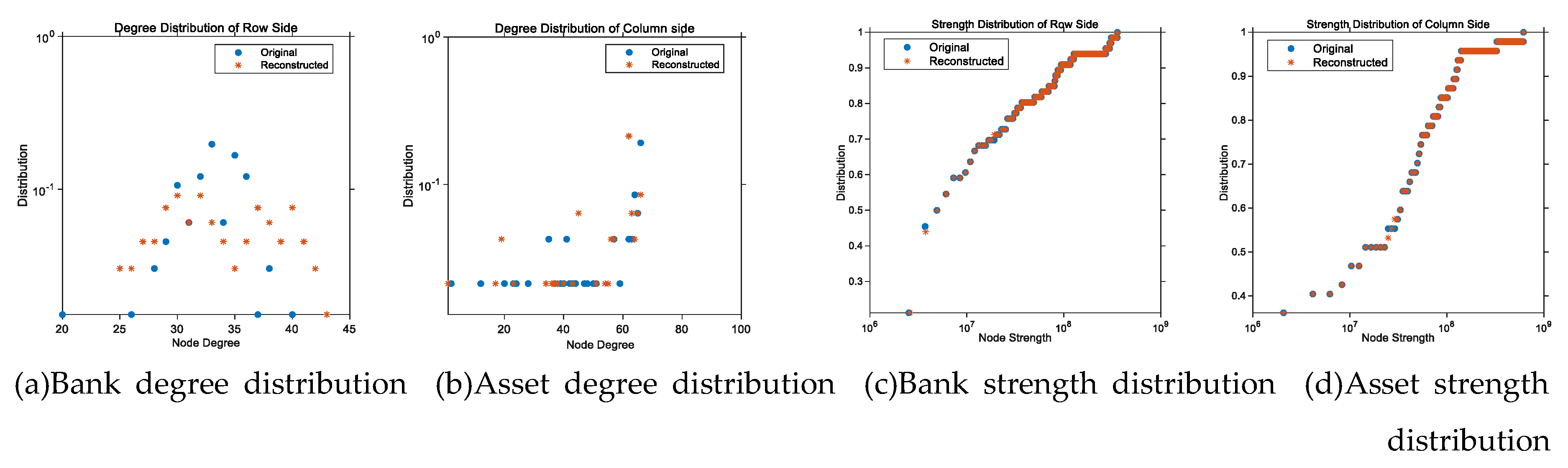
• Degree distribution and Strength distribution

As illustrated in Table 3, from 2016 to 2022, the average degree of the actual network ranged between$\overline{{\mathrm{k}}_{\mathrm{o}}}\text{∈}[19.15,22.48]$, while that of the reconstructed network ranged between$\overline{{\mathrm{k}}_{\mathrm{r}}}\text{∈}[19.68,23.00]$. The annual average degree error is less than$|\overline{{\mathrm{k}}_{\mathrm{o}}}-\overline{{\mathrm{k}}_{\mathrm{r}}}|\text{<}0.7$, demonstrating a favorable goodness-of-fit. As depicted in Figure 3, the degree distribution of bank nodes follows a power-law pattern, while the degree of asset nodes exhibits a stepwise distribution. The figures show that large banks hold a dominant position in terms of asset scale, with a prominent cumulative effect in the network tail, thereby confirming the scale-free characteristics of the network. In terms of both node degree distribution and strength distribution, the reconstructed network closely approximates the characteristics of the empirical network. The fit is particularly strong for node strength, indicating the model’s efficacy in capturing the core properties of the real-world system.

2.

Network density, clustering coefficient, and degree correlation

As shown in Table 3, between 2016 and 2022, the density of both actual and reconstructed networks ranged between${\mathrm{D}}_1\text{∈}[0.70,0.75]$and${\mathrm{D}}_2\text{∈}[0.72,0.77]$ respectively. The relatively high network density indicates that banks maintain broad coverage across asset categories. However, a discernible trend of decreasing density over time highlights an increasing concentration in the types of assets held by banks. This sparsification phenomenon may be associated with the tightening of asset management regulations during this period. Notably, city commercial banks and small-to-medium sized banks exhibited a more pronounced concentration in their asset holdings compared to larger institutions. During this period, the network clustering coefficient lies in the interval $\mathrm{C}\text{∈}[0.7,0.8]$, which is significantly higher than that of a random network of equivalent scale. Furthermore, the degree correlation for both the actual and reconstructed networks is negative. This disassortative mixing pattern indicates that bank nodes with a high degree, holding many asset types, are connected to asset nodes with a low degree, held by few banks, and vice versa. This structural characteristic suggests a divergence in asset allocation strategies, small and medium-sized banks in China exhibit a stronger preference for regulatory-compliant assets and mainstream deposit and loan businesses, whereas large state-owned banks maintain a more diversified asset portfolio.

3.

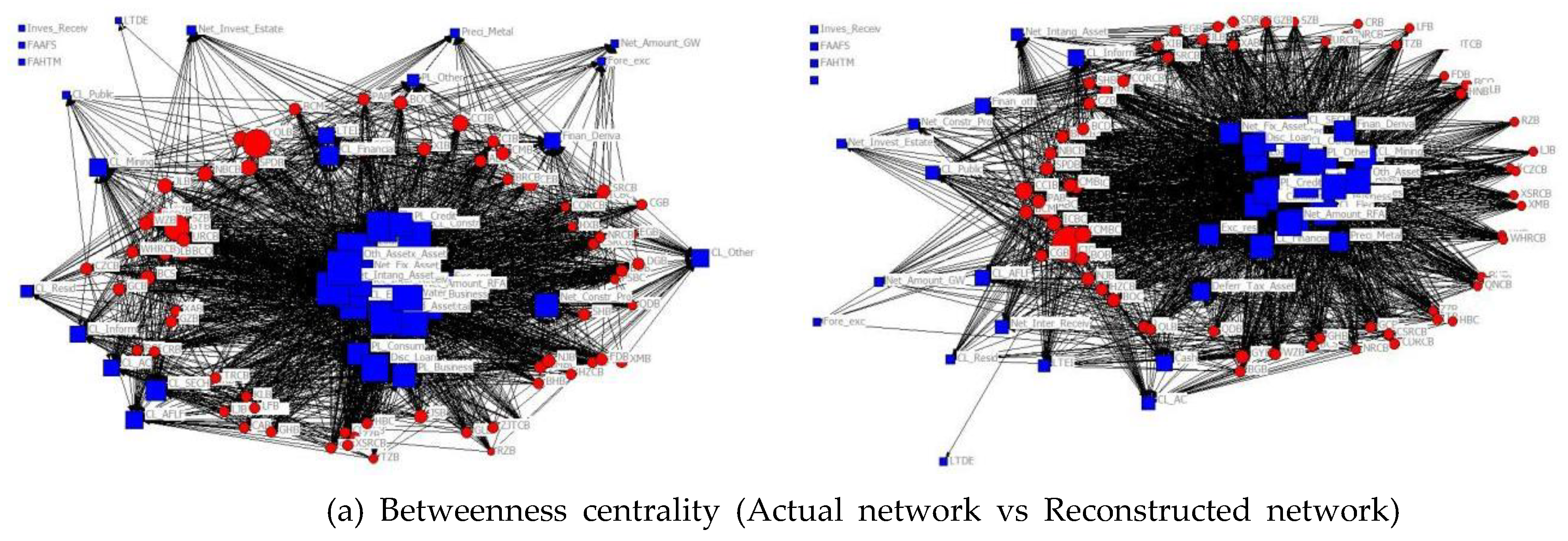
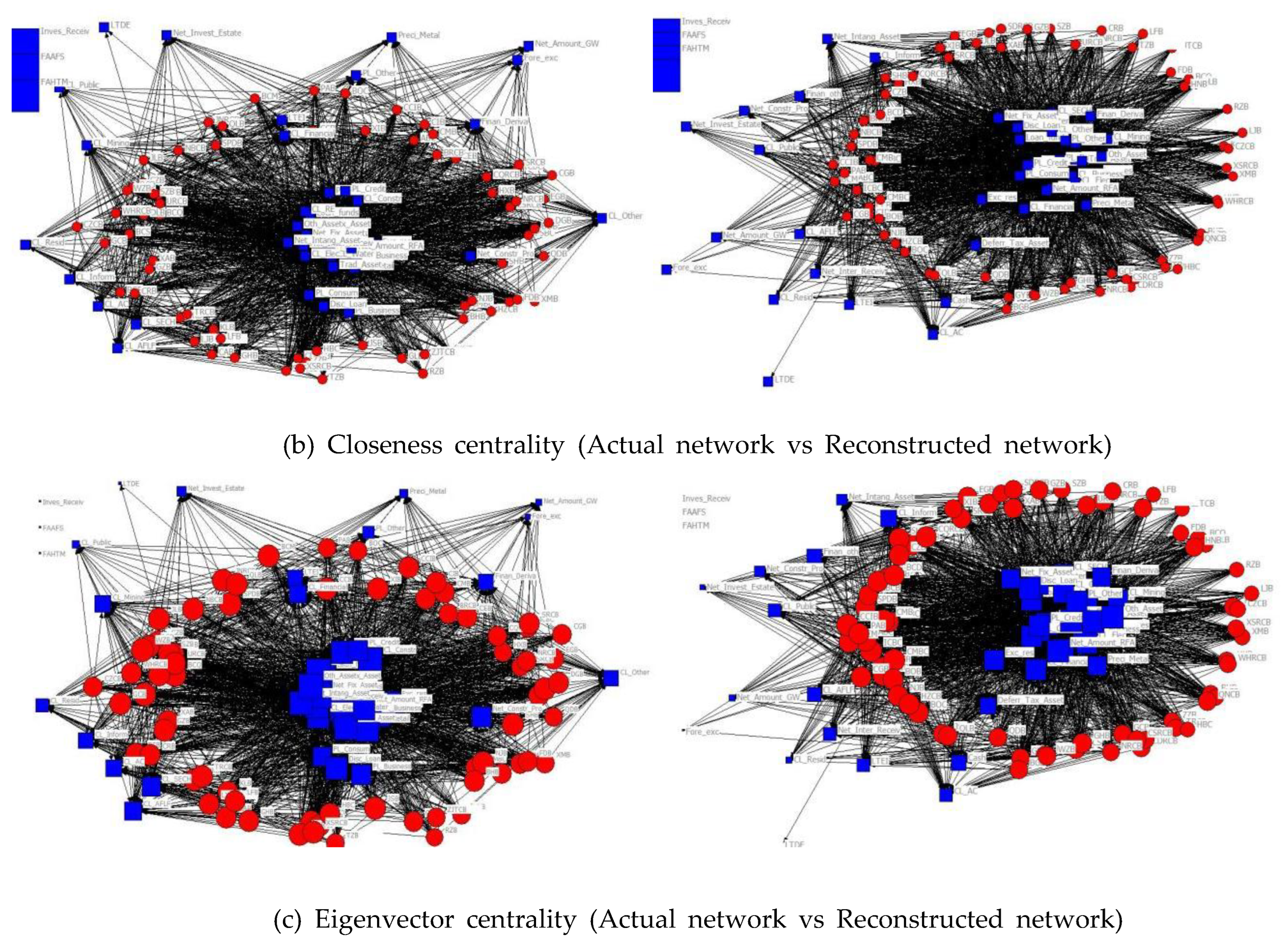
Betweenness centrality, Closeness centrality, and Eigenvector centrality

Network centrality indicators are crucial for assessing node importance within a system. We employ three standard centrality measures, betweenness centrality, closeness centrality, and eigenvector centrality, to analyze the specific features of both the actual and reconstructed networks. Figure 4 compares the values of these three centrality indicators for the actual and reconstructed bank-asset networks in 2022. In the figure, bank nodes and asset nodes are represented by red circles and blue rectangles, respectively. The size of each node is proportional to its centrality value, visually indicating its relative importance within the network system.

As shown in Figure 4, the topological distribution of node centrality values in the reconstructed network exhibits characteristics highly consistent with the actual network, both in terms of value distribution and node categorization. Regarding betweenness centrality in Figure 4(a), asset nodes generally possess higher values than bank nodes. The betweenness centrality of most asset nodes falls within a similar magnitude, whereas only a small fraction of bank nodes exhibit significantly higher values than their peers. In contrast, for closeness centrality in Figure 4(b), the values for both asset and bank nodes are of a comparable magnitude, indicating that most nodes are of approximately equal importance in terms of their network proximity. Concerning eigenvector centrality in Figure 4(c), most asset nodes exhibit relatively large values, compared with those of bank nodes. Furthermore, the eigenvector centrality values are nearly uniform across almost all bank nodes. Overall, a comparison of node centrality between the actual and reconstructed networks reveals that the latter captures the overall distribution of node centrality with a high degree of accuracy, with only marginal discrepancies observed in a limited number of individual nodes. This finding underscores the efficacy of the weight-based link allocation strategy employed in the network reconstruction methodology.

4.

Asset concentration

Figure 5 displays heatmaps of the Herfindahl-Hirschman Index (HHI) distribution for bank and asset nodes in both the actual and reconstructed bank-asset allocation networks from 2016 to 2022. In the heatmaps, node color corresponds to HHI value, where red indicates a value of $\mathrm{HHI}=1$, blue indicates a value of $\mathrm{HHI}=0$, and a gradient represents the spectrum in between. Isolated nodes, for which the HHI is undefined, are represented by white space.

Figure 5(a) and Figure 5(b) show the Assets’ HHI in actual network and reconstructed network. While Figure 5(c) and Figure 5(d) display the Banks’ HHI in actual and reconstructed network accordingly. As shown in Figure 5(a) and Figure 5(b), the HHI of asset nodes in the actual and reconstructed networks ranged between${\mathrm{HHI}}_{\mathrm{m}1}\text{∈}[0,0.75)$ and ${\mathrm{HHI}}_{\mathrm{m}2}\text{∈}[0,1]$ from 2016 to 2022. In the actual network, most asset nodes’ HHI values exhibit fluctuating around 0.1, indicating a relatively extensive and diversified distribution of assets across the banking system. In contrast, Figure 5(c) and Figure 5(d) show that the HHI of bank nodes in the actual and reconstructed networks ranged between${\mathrm{HHI}}_{\mathrm{b}1}\text{∈}[0,0.30)$and ${\mathrm{HHI}}_{\mathrm{b}2}\text{∈}[0,0.12)$. The heatmaps for the actual network reveal significant heterogeneity in asset concentration among banks. Compared with large state-owned commercial banks and national joint-stock commercial banks, urban and rural commercial banks tend to exhibit weaker investment concentration (lower HHI). Overall, the banks’ HHI demonstrate a gentle upward trend from 2016 to 2022, reflecting a gradual increase in asset concentration within individual banks’ portfolios. This trend toward more concentrated asset allocation is consistent with the previously observed evolutionary characteristics of decreasing network density and varying node degree distribution.

3.2.3. Similarity measurement

To evaluate the macro-level similarity between the reconstructed and actual networks, we employ two commonly used measures [28], the Jaccard score (a link-based measure) and the Cosine similarity (an exposure-based measure), as shown in Table 4. For both metrics, the higher values are, the greater the similarity between the networks.

Table 5 shows the result of the similarity measurements between the actual and reconstructed network. The Jaccard similarity value falls within the interval$[0.65,0.72]$, indicating that the reconstructed network achieves a high fitness score in replicating the binary linkage structure between nodes. In terms of strength allocation, the Cosine similarity value lies in the interval$[0.87,0.96]$, reflecting a high degree of similarity in edge weight distribution between the two networks. This performance exceeds the fit level achieved by the bank-enterprise credit reconstruction network proposed by Ramadiah et al. [32].

4. Simulation Study

Based on the reconstructed bank-asset network and the proposed vulnerability measurement framework, we conduct a simulation analysis to examine how risk contagion propagates and amplifies systemic vulnerability. The simulation analysis incorporates the following key parameters: network size, risk exposure, leverage, external shock, asset price impact, and fire-sales effect. Network size and risk exposure parameters are derived directly from the reconstructed network. The leverage threshold is set as a fixed value of LEV=4%. A bank is considered insolvent if the depreciation of its assets causes its capital adequacy ratio to fall below this threshold $\mathsf{\chi }=5\%$. When the rate of bank insolvencies exceeds a predefined threshold(i.e., the initial bankruptcy rate triggered by the external shock), it triggers an asset price price impact mechanism. This mechanism simulates the price decline resulting from forced liquidation and fire sales. The external shock rate is parameterized as$\mathrm{q}\text{∈}[0,1]$ and the fire-sales price impact coefficient is denoted by $\mathsf{\xi }\text{∈}[0.05,0.1]$.

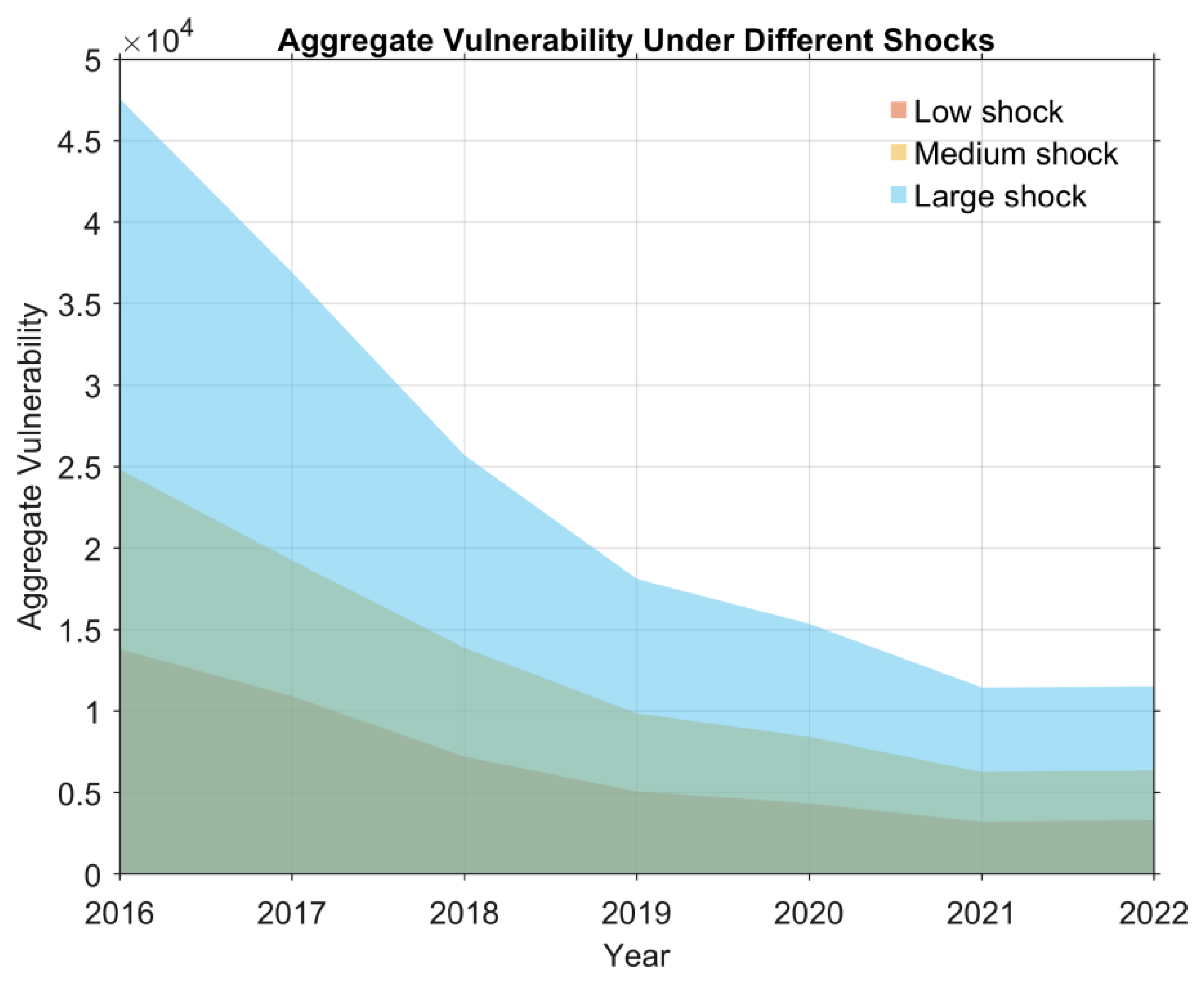
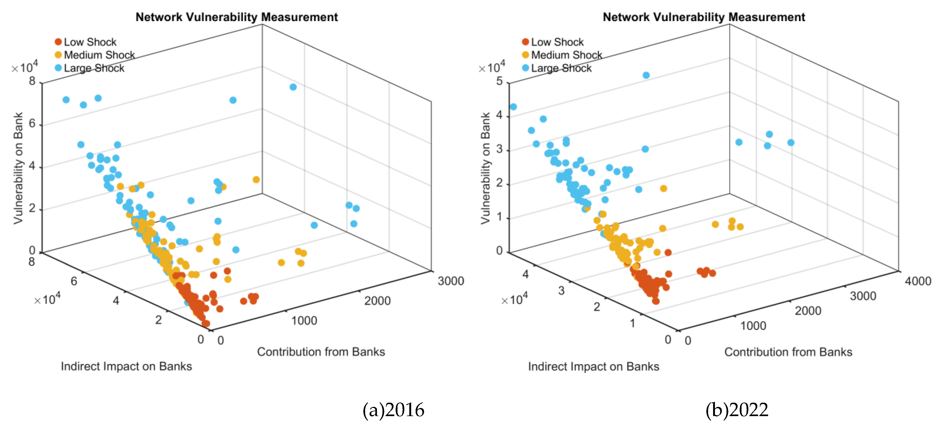
4.1. Measuring network aggregate vulnerability

Let the external shock rate be defined by the parameter $\mathrm{q}$, we consider three benchmark values for it(low, medium, high), and for each, we generate a corresponding set of random initial external shocks, which are $\mathrm{q}=15\%$,$\mathrm{q}=25\%$ and $\mathrm{q}=35\%$ respectively. Following the aggregate vulnerability equation, we compute the aggregate vulnerability${\mathrm{AV}=1}_{\mathrm{N}}^{\text{'}}{\mathrm{A}}_1\mathrm{M}\mathsf{\xi }\mathrm{M}\text{'}\mathrm{B}{\mathrm{A}}_1\mathrm{Mq}/{\mathrm{E}}_0$under each shock scenario. This metric quantifies the cumulative losses from risk contagion caused by bank deleveraging and asset fire sales, expressed as the percentage of total banking sector equity that would be eroded. Holding all other parameters at their default values, we conduct the simulation analysis to measure network vulnerability for each year from 2016 to 2022 as follows.

Figure 6 depicts the vulnerability of bank-asset network under different initial external shock scenarios from 2016 to 2022. Overall, the trajectory of network vulnerability is consistent across this period, with the magnitude of equity erosion generally decreasing over time. Under the three shock scenarios, the aggregate network maintained a relatively constant loss level from 2020 to 2022, showing no sharp increases or decreases despite variations in shock intensity. In contrast, the aggregate losses were significantly higher between 2016 and 2019 than that in the subsequent three-year period. The network aggregate vulnerability${\mathrm{AV}*{\mathrm{E}}_0=1}_{\mathrm{N}}^{\text{'}}{\mathrm{A}}_1\mathrm{M}\mathsf{\xi }\mathrm{M}\text{'}\mathrm{B}{\mathrm{A}}_1\mathrm{Mq}=\sum _{\mathrm{n}}{\mathsf{\gamma }}_{\mathrm{n}}{\mathrm{b}}_{\mathrm{n}}{\mathrm{a}}_{\mathrm{n}0}{\mathrm{r}}_{\mathrm{n}0}$can be formally expressed by the equation${\mathrm{AV}=1}_{\mathrm{N}}^{\text{'}}{\mathrm{A}}_1\mathrm{M}\mathsf{\xi }\mathrm{M}\text{'}\mathrm{B}{\mathrm{A}}_1\mathrm{Mq}/{\mathrm{E}}_0$, where${\mathsf{\gamma }}_{\mathrm{n}}={\sum }_{\mathrm{k}}\left({\sum }_{\mathrm{m}}{\mathrm{a}}_{\mathrm{m}}{\mathrm{m}}_{\mathrm{mk}}\right){\mathrm{l}}_{\mathrm{k}}{\mathrm{m}}_{\mathrm{nk}}$ measures the connection among banks. According to this formulation, systemic risk increases with larger values of network structure${\mathrm{a}}_{\mathrm{n}0}$, leverage${\mathrm{b}}_{\mathrm{n}0}$, and risk exposure${\mathrm{r}}_{\mathrm{n}0}$. This implies that systemic vulnerability is amplified when large, highly leveraged banks are exposed to a shock, triggering substantial asset sales. Furthermore, if these exposed banks hold illiquid assets, the resulting large price impact can render the entire network system more vulnerable.

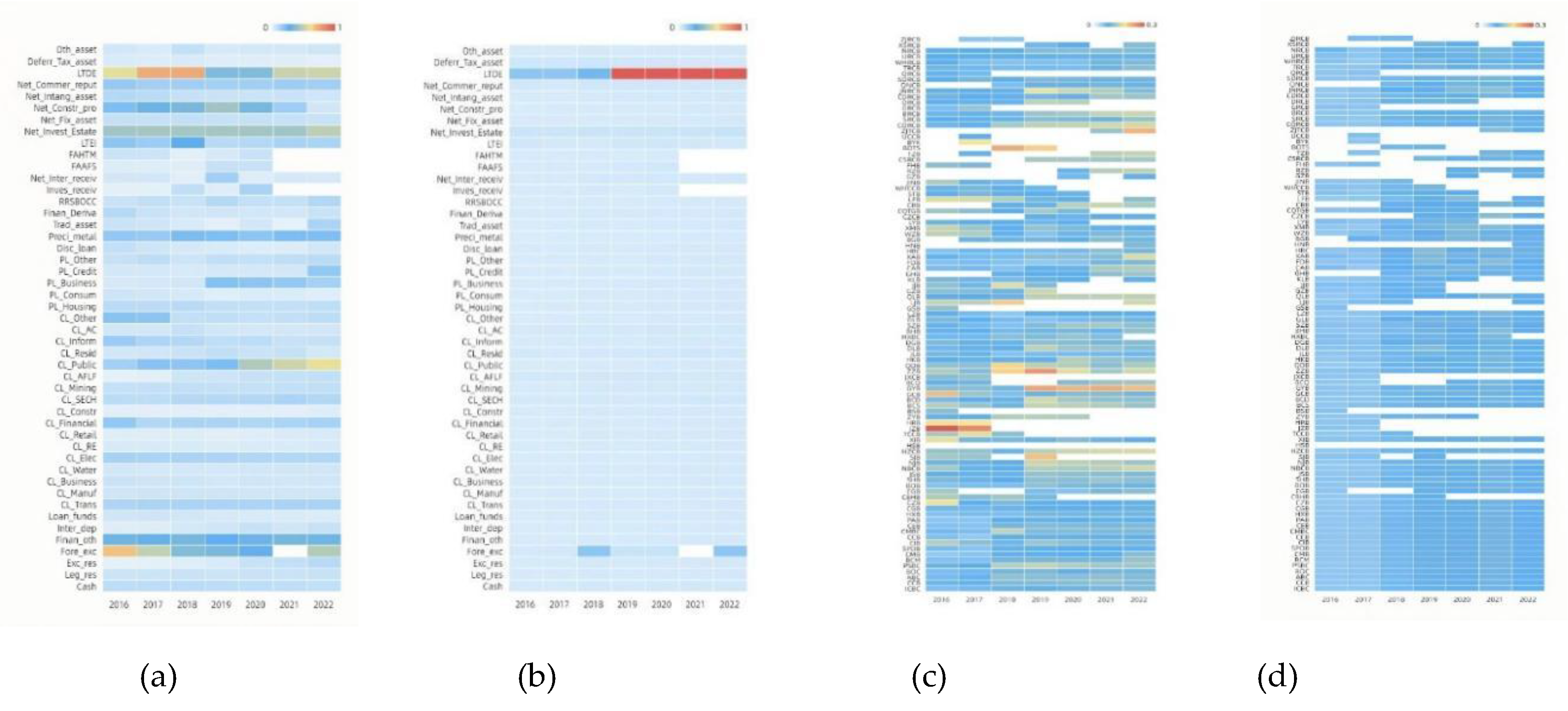
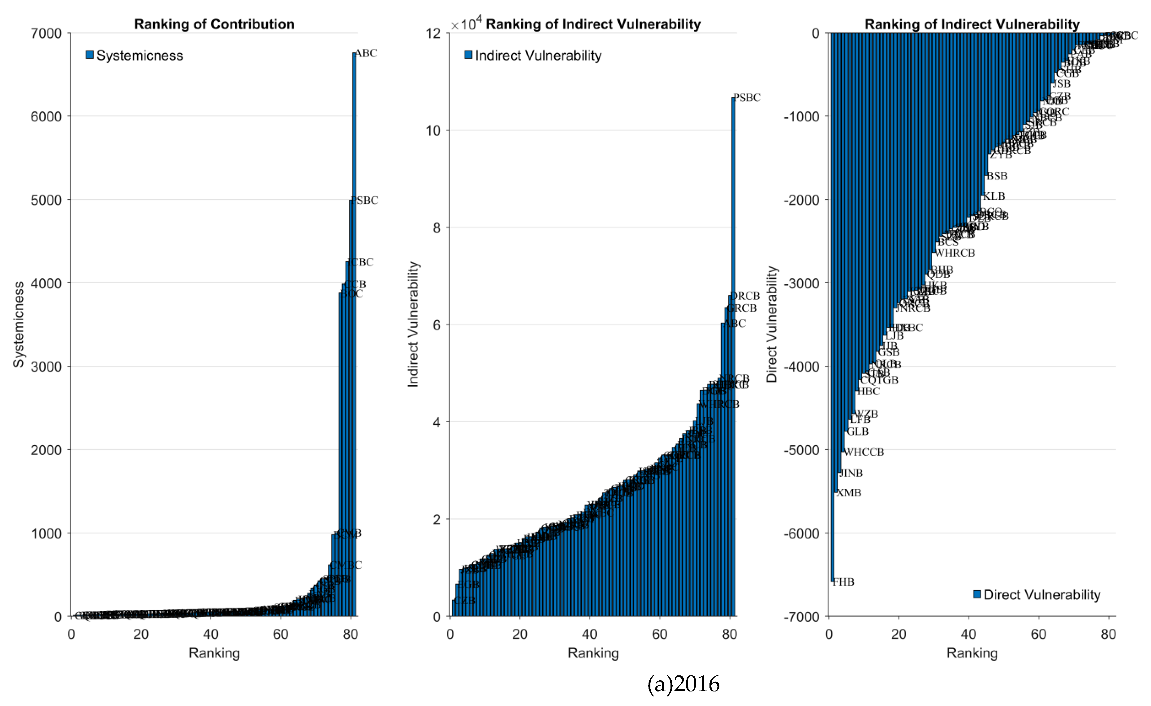
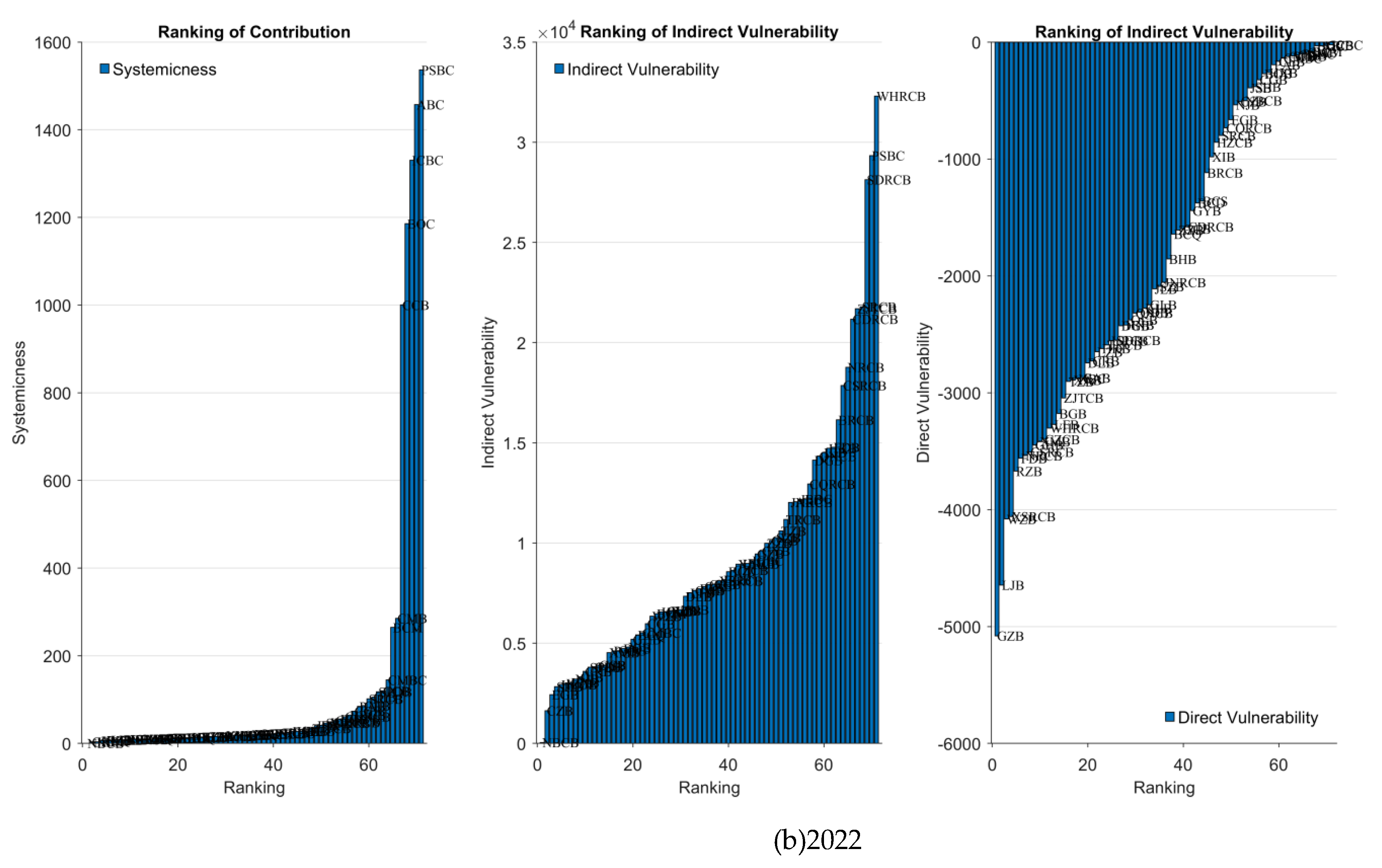
4.2. Contribution from each bank to network vulnerability

Building upon the analysis of aggregate network vulnerability, which quantifies the cumulative losses arising from bank inter-dependencies and dynamic behaviors during risk contagion under external shocks, we can decompose this systemic measure into individual bank contributions. This aggregate vulnerability can be viewed as the sum of contributions from individual nodes, transmitted through fire sale spillover effects across the banking system. Therefore, we can calculate the vulnerability contribution of each bank, which serves as an indicator of its systemic importance within the network. The systemic impact of an individual bank$\mathrm{i}$ on the banking network can be quantified by calculating the marginal contribution${{\mathrm{SI}}_{\mathrm{i}}=1}_{\mathrm{N}}^{\text{'}}{\mathrm{A}}_1\mathrm{M}\mathsf{\xi }\mathrm{M}\text{'}\mathrm{B}{\mathrm{A}}_1{\mathsf{\delta }}_{\mathrm{i}}{\mathsf{\delta }}_{\mathrm{i}}^{\mathrm{\text{'}}}\mathrm{Mq}/{\mathrm{E}}_{\mathrm{i}}$, where${\mathsf{\delta }}_{\mathrm{i}}$ is a shock vector consisting of all zeros except for the $\mathrm{i}-\mathrm{th}$ element, which is set to 1. This represents the hypothetical aggregate vulnerability triggered by an initial shock exclusively to bank $\mathrm{i}$. Consistent with the formulation of aggregate vulnerability$\mathrm{AV}$, the individual contribution${{\mathrm{SI}}_{\mathrm{i}}=1}_{\mathrm{N}}^{\text{'}}{\mathrm{A}}_1\mathrm{M}\mathsf{\xi }\mathrm{M}\text{'}\mathrm{B}{\mathrm{A}}_1{\mathsf{\delta }}_{\mathrm{i}}{\mathsf{\delta }}_{\mathrm{i}}^{\mathrm{\text{'}}}\mathrm{Mq}/{\mathrm{E}}_{\mathrm{i}}$ can be similarly transformed into a function${\mathrm{SI}}_{\mathrm{i}}={\mathsf{\gamma }}_{\mathrm{i}}{({\mathrm{a}}_{\mathrm{i}1}/{\mathrm{E}}_{\mathrm{i}})\mathrm{b}}_{\mathrm{i}}{\mathrm{r}}_{\mathrm{i}1}$with the key network parameters. Building on this measure of individual bank loss contribution${\mathrm{SI}}_{\mathrm{i}}$, we conduct a simulation analysis from 2016 to 2022 to examine the correlations between the following three key metrics: a bank’s systemic importance${\mathrm{SI}}_{\mathrm{i}}$, a bank’s individual systemic vulnerability$\mathrm{DV}$, and the overall network aggregate vulnerability$\mathrm{A}\mathrm{V}$. This analysis characterizes how the behavioral states and financial conditions of individual network entities influence the propagation of risk contagion and the amplification of cumulative losses.

As shown in Figure 7, no direct linear relationship exists between systemically important banks and systemically vulnerable banks. This indicates that large, top-tier banks do not necessarily play the most critical role in risk propagation; conversely, smaller banks can also be exposed to significant indirect risks through contagion channels, even without experiencing direct shocks. Figure 7(a) demonstrates that under a low-magnitude external shock, banks with dense interconnections can rapidly transmit risks throughout the system. Figure 7(b) reveals that although the overall level of risk spillover from systemically vulnerable banks has decreased, their marginal risk contribution remains more significant than that observed in the dimension of systemic importance. This suggests that well-connected, vulnerable banks play a disproportionately large role in amplifying risk contagion processes.

Figure 8 shows the distribution of individual banks’ contributions to aggregate network vulnerability in 2016 and 2022. The figure reveals that most banks contribute at a low level to systemic vulnerability under cumulative risk contagion, while only a small subset exhibited high risk exposure. The significant heterogeneity among bank nodes and the scale-free structure of the network highlight that identifying these systemically important nodes be crucial for effective systemic risk prevention. From the perspective of individual node risk, the difference in risk contribution from systemically important banks between 2016 and 2022 is not pronounced. However, the analysis confirms that larger initial shocks lead to more significant risk accumulation effects propagated by these systemically important banks. In the network visualization, node color indicates risk spillover intensity: yellow nodes represent the highest level of risk spillover, followed by nodes of other colors. This depiction reflects not only the differential risk losses arising from variations in initial shocks but also validates the heterogeneity in node sizes and the core-periphery topological structure of the banking network. This structural pattern is consistent with the long-term configuration of China’s banking sector, which is dominated by six large state-owned banks and features a multi-polar distribution of twelve national joint-stock commercial banks. Furthermore, compared to the measure of systemic importance, the systemic vulnerability of bank nodes demonstrates a wider and more stratified hierarchical distribution, indicating a more complex pattern of risk exposure across the system.

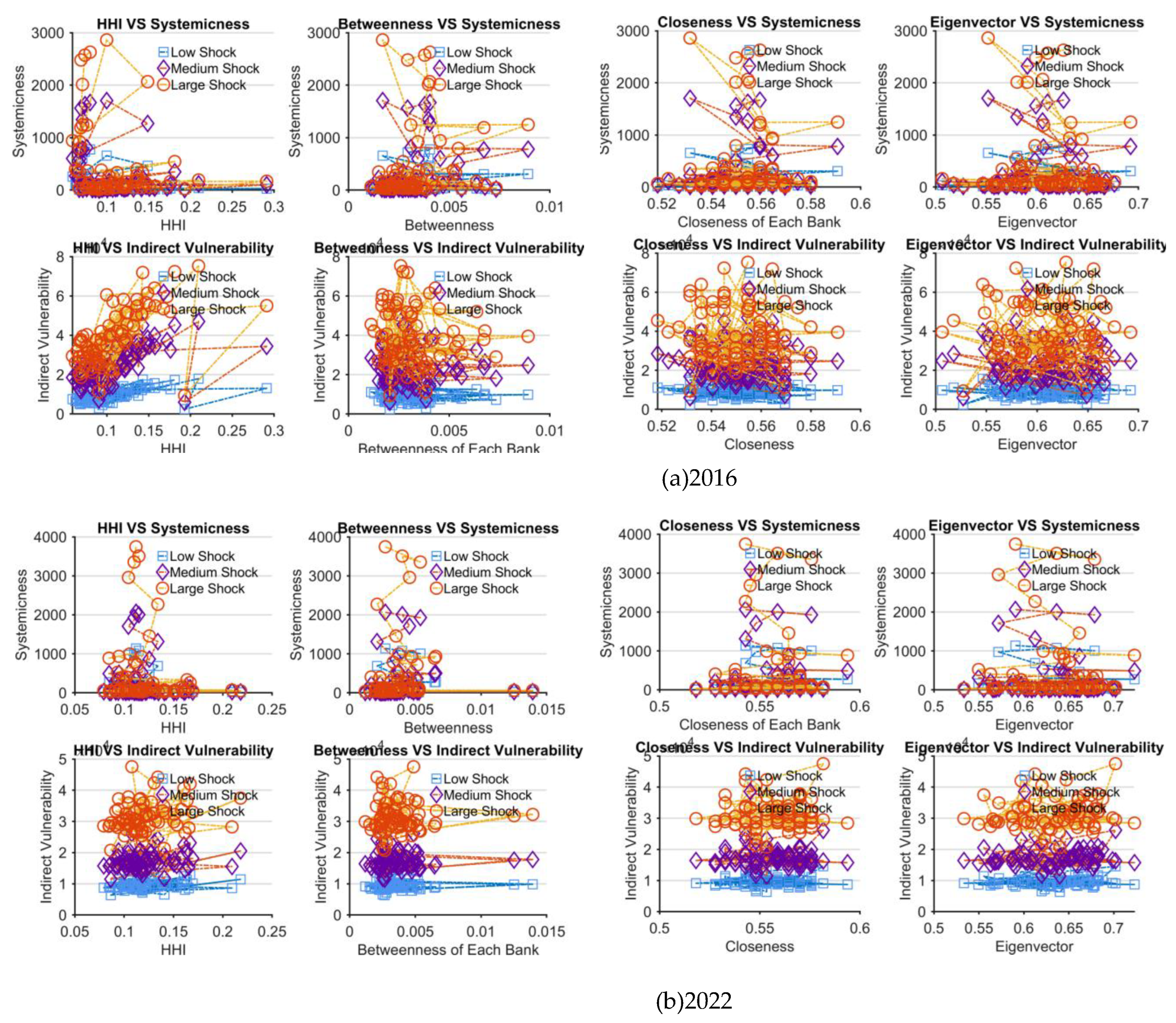
4.3. Network topology structure on network vulnerability

As indicated in aggregate vulnerability measurement ${\mathrm{AV}*{\mathrm{E}}_0=1}_{\mathrm{N}}^{\text{'}}{\mathrm{A}}_1\mathrm{M}\mathsf{\xi }\mathrm{M}\text{'}\mathrm{B}{\mathrm{A}}_1\mathrm{Mq}=\sum _{\mathrm{n}}{\mathrm{r}}_{\mathrm{n}}{\mathrm{b}}_{\mathrm{n}}{\mathrm{a}}_{\mathrm{n}0}{\mathrm{r}}_{\mathrm{n}0}$, network structure serves as a critical indicator of banks’ asset allocation, emerging as a pivotal determinant governing the cumulative losses incurred within networked systems. Building on the preceding analysis, We select four network topological indicators, HHI of banks’ asset concentration, betweenness centrality, closeness centrality, and eigenvector centrality, to examine their intrinsic relationships with two key dependent variables, which are banks’ indirect vulnerability from risk contagion (I$\mathrm{V}$), and contribution to aggregate systemic vulnerability(S$\mathrm{V}$).

Figure 9(a) and Figure 9(b) show the correlations between network topology metrics and node vulnerability indicators for 2016 and 2022, respectively. The figures indicate that, in both years, no significant linear relationship exists between the four network topological indicators and the vulnerability of individual nodes. The contributions of bank nodes to the cumulative systemic vulnerability varied substantially, with a subset of nodes exhibiting disproportionately high risk contribution. In contrast, the distribution of losses across banks affected by risk contagion demonstrated a relatively low dispersion under identical shock conditions. At the network level, as the concentration of bank asset investments increases (i.e., distribution tightened), aggregate systemic vulnerability exhibits a slight downward trend. This finding is consistent with the previously observed sparsification of network density and node degree, suggesting that reduced connectivity within the bank-asset network decreases the number of available risk transmission paths, thereby weakening risk spillover and diffusion effects. This is further corroborated by the significant decline in the risk spillover contribution from systemically vulnerable banks. Regarding centrality metrics, the centrality of bank nodes demonstrates greater efficacy in identifying systemically vulnerable banks, a role that is often modulated by the magnitude of external shocks. As node centrality increases, both$\mathrm{SV}$ and $\mathrm{IV}$ tend to exhibit extreme values, enabling the effective identification of key nodes that contribute significantly to systemic risk. This underscores the advantage of centrality measures in characterizing both the systemic importance and vulnerability of banks within the network.

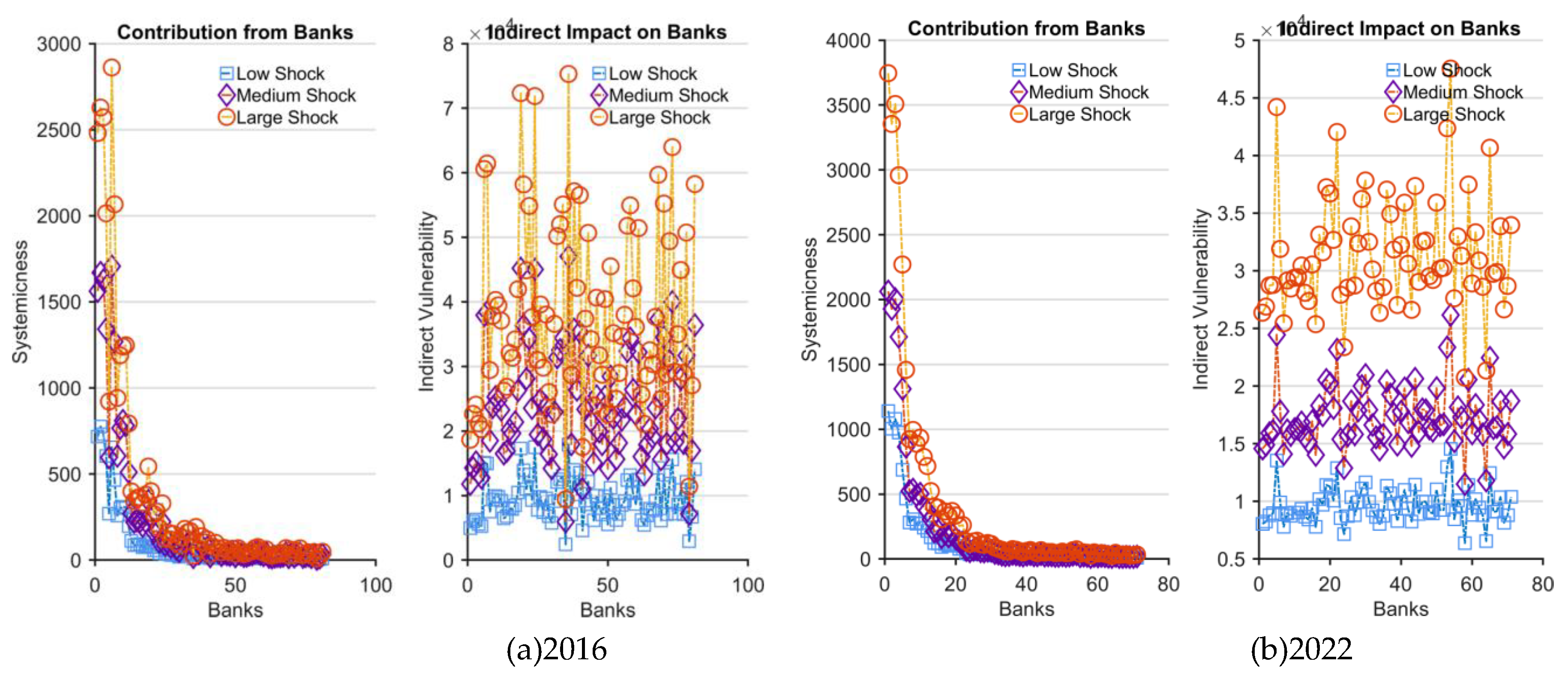
4.4. Impact of risk contagion on individual banks

Based on the network vulnerability measurement model and its analysis framework, we define two vulnerability indicators for individual bank nodes, named direct vulnerability$\mathrm{D}\mathrm{V}$and indirect vulnerability$\mathrm{IV}$, to quantify their risk exposure from contagion triggered by exogenous initial shocks. The indirect vulnerability metric$\mathrm{IV}$ specifically quantifies the risk exposure arising from the combined effect of network-wide deleveraging and the topological connections between nodes. It is a distinct concept from both direct vulnerability and a node’s systemic importance. Thus, using 2016 and 2022 as representative examples, we calculate and rank the risk vulnerability of all bank nodes for each year. This ranking aims to depict the characteristics of the risk distribution and identify the nodes most susceptible to contagion effects.

Figure 10 presents the ranking distributions of direct risk losses, indirect risk vulnerability, and network system vulnerability contribution from bank nodes in the bank-asset allocation network for 2016 and 2022, under a low external shock scenario. Additionally, the top 10 nodes ranked by indirect risk vulnerability and systemic vulnerability contribution are detailed in Table 6. As shown in Fig.10, the distributions of both indirect risk vulnerability and systemic vulnerability contribution exhibit a typical heavy-tailed pattern in both years, indicating that a small number of banks account for a disproportionately large share of the systemic risk. The composition of the top 10 banks by systemic vulnerability contribution, listed in Table6, remains consistent between 2016 and 2022, with only minor variations in their ordinal rankings. These banks are exclusively state-owned banks and leading national joint-stock commercial banks. This consistency underscores the prominent systemic importance of China’s large state-owned commercial banks. Their significant contribution to systemic vulnerability stems from their substantial asset scale, high degree of interconnectedness, and the diversity of their asset allocations.

Conversely, the composition of the top 10 banks ranked by indirect vulnerability exhibits significant turnover between 2016 and 2022. With the exception of the Postal Savings Bank of China, the lists for the two years show almost no overlap. These top ranked vulnerable banks are predominantly rural commercial banks and small-medium-sized urban commercial banks. This finding indicates that the correlation stemming from holding common asset portfolios is a primary driver of risk vulnerability at the node level. Furthermore, the role of highly central nodes in amplifying cumulative systemic vulnerability through risk contagion is particularly significant. These results imply that the optimal design of banking regulatory strategies must incorporate a dual focus: the traditional “too big to fail” principle and a “too connected to fail” principle, which accounts for the critical role of interconnectedness and common asset exposures in propagating systemic risk.

5. Conclusions

The multifaceted interactions between financial institutions can be considered as a complex network. Given the multi-channel nature of risk contagion within the bank-asset system, this study employs network theory to identify these financial linkages and characterize systemic risk and financial stability. Using balance sheet data from Chinese commercial banks from 2016 to 2022, we apply Exponential Random Graph Models to reconstruct the bipartite network of bank-asset holdings, replicating the topology of the empirical banking system. We then propose a novel framework to measure network aggregate vulnerability, incorporating factors such as bank size, initial shocks, interconnectedness, leverage, and asset fire sales to model financial contagion. Within this framework, we define a suite of network-based vulnerability metrics: network aggregate vulnerability$\mathrm{AV}$ (system-wide cumulative loss due to risk contagion), direct vulnerability$\mathrm{DV}$ (a bank’s immediate losses from an initial shock), indirect vulnerability$\mathrm{IV}$ (a bank’s losses propagated through network contagion), systemic contribution$\mathrm{SV}$ (a bank’s contribution to aggregate vulnerability). We subsequently conduct a simulation analysis to examine the dynamics of bank-asset network vulnerability under varying levels of external shocks. The key findings from the simulation analysis are as follows:

(1)Utilizing balance sheet data from Chinese commercial banks from 2016 to 2022, we construct a bank-asset allocation network that exhibits distinct scale-free properties and a high clustering coefficient. Unlike the sparsity typical of most real-world financial networks, the reconstructed network demonstrates greater density and a disassortative mixing pattern. Banks within this network maintain holdings of statutory assets while also displaying a broad tendency to invest in credit and financial investment assets. The nodes representing large state-owned and joint-stock commercial banks exhibit higher degrees, reflecting their typical diversity in asset allocation. The dense interconnections between assets provide potential channels for risk contagion. Furthermore, the disassortative nature of the network, where highly connected banks hold less popular assets, means that shocks to these low-degree assets can be amplified through their connections to major banks, thereby increasing systemic vulnerability.

(2)The commercial bank asset allocation network, reconstructed by Exponential Random Graph Models, effectively replicates the macro-level topological structure of the real-world bipartite bank-asset network. The model demonstrates a particularly strong goodness-of-fit in replicating the distribution of edge weights. Quantitative similarity measurements confirm this result. The Jaccard index for network edge reconstruction ranges between$[0.65,0.72]$, indicating a high degree of accuracy in replicating the binary linkage structure between nodes. Furthermore, the Cosine similarity, an exposure-based measure for link weights, ranges between$[0.87,0.96]$, reflecting a high fidelity in replicating the edge weight distribution between the actual and reconstructed networks from 2016 to 2022. At the micro-level, the theoretically reconstructed network model accurately replicates key topological metrics, including network density, node degree distribution, clustering coefficient, and degree-degree correlation, confirming its robustness in capturing the detailed structural characteristics of the empirical system.

(3)Simulation analysis reveals that varying levels of initial external shocks exert distinct effects on risk contagion and systemic vulnerability within the bank-asset network. From 2016 to 2022, the aggregate vulnerability of the network exhibited a general declining trend. Annually, the cumulative aggregate vulnerability increases non-linearly with the magnitude of the initial negative shock and the discount rate applied during asset fire sales. The indirect vulnerability for individual banks, resulting from contagion triggered by deleveraging and fire sales, is substantially higher than the direct losses caused by the initial shocks themselves. The contribution to cumulative systemic vulnerability is predominantly concentrated in large state-owned banks and national joint-stock commercial banks due to their substantial asset sizes. In contrast, the institutions most severely affected by the resulting risk shocks are predominantly small-medium-sized rural and urban commercial banks.

Appendix A.1

Table A1. Bank Nodes.

Bank Abbreviation	Bank Name	Category
ICBC	Industrial and Commercial Bank of China	State-Owned Large Commercial Bank
CCB	China Construction Bank	State-Owned Large Commercial Bank
ABC	Agricultural Bank of China	State-Owned Large Commercial Bank
BOC	Bank of China	State-Owned Large Commercial Bank
PSBC	Postal Savings Bank of China	State-Owned Large Commercial Bank
BCM	Bank of Communications	State-Owned Large Commercial Bank
CMB	China Merchants Bank	National Joint-Stock Commercial Bank
SPDB	Shanghai Pudong Development Bank	National Joint-Stock Commercial Bank
CIB	China's Industrial Bank	National Joint-Stock Commercial Bank
CCIB	China CITIC Bank	National Joint-Stock Commercial Bank
CMBC	China Minsheng Bank	National Joint-Stock Commercial Bank
CEB	China Everbright Bank	National Joint-Stock Commercial Bank
PAB	Ping An Bank	National Joint-Stock Commercial Bank
HXB	Huaxia Bank	National Joint-Stock Commercial Bank
CGB	China Guangfa Bank	National Joint-Stock Commercial Bank
CZB	China Zheshang Bank	National Joint-Stock Commercial Bank
CBHB	China Bohai Bank	National Joint-Stock Commercial Bank
EGB	Evergrowing Bank	National Joint-Stock Commercial Bank
BOB	Bank of Beijing	City Commercial Bank
SHB	Bank of Shanghai	City Commercial Bank
JSB	Bank of Jiangsu	City Commercial Bank
NBCB	Bank of Ningbo	City Commercial Bank
NJB	Bank of Nanjing	City Commercial Bank
SJB	Shengjing Bank	City Commercial Bank
HZCB	Bank of Hangzhou	City Commercial Bank
HSB	Huishang Bank	City Commercial Bank
XIB	Xiamen International Bank	City Commercial Bank
TCCB	Tianjin City Commercial Bank	City Commercial Bank
JZB	Bank of Jinzhou	City Commercial Bank
HRB	Harbin Bank	City Commercial Bank
ZYB	Bank of Zhongyuan	City Commercial Bank
BSB	Baoshang Bank	City Commercial Bank
BCS	Bank of Changsha	City Commercial Bank
BCD	Bank of Chengdu	City Commercial Bank
GCB	Bank of Guangzhou	City Commercial Bank
GYB	Bank of Guiyang	City Commercial Bank
BCQ	Bank of Chongqing	City Commercial Bank
JXCB	Bank of Jiangxi	City Commercial Bank
ZZB	Bank of Zhengzhou	City Commercial Bank
QDB	Bank of Qingdao	City Commercial Bank
HKB	Bank of Hankou	City Commercial Bank
JLB	Bank of Jilin	City Commercial Bank
DLB	Bank of Dalian	City Commercial Bank
DGB	Bank of Dongguan	City Commercial Bank
HXBC	Huarong Xiangjiang Bank	City Commercial Bank
BHB	Bank of Hebei	City Commercial Bank
SZB	Bank of Suzhou	City Commercial Bank
GLB	Bank of Guilin	City Commercial Bank
LZB	Bank of Lanzhou	City Commercial Bank
GSB	Gansu Bank	City Commercial Bank
LJB	Longjiang Bank	City Commercial Bank
QLB	Qilu Bank	City Commercial Bank
GZB	Guizhou Bank	City Commercial Bank
JJB	Jiujiang Bank	City Commercial Bank
KLB	Kunlun Bank	City Commercial Bank
GHB	Guangdong Huaxing Bank	City Commercial Bank
CAB	Chang’an Bank	City Commercial Bank
FDB	Fudian Bank	City Commercial Bank
XAB	Xi’an Bank	City Commercial Bank
HBC	Hubei Bank	City Commercial Bank
HNB	Hunan Bank	City Commercial Bank
BGB	Guangxi Beibu Gulf Bank	City Commercial Bank
WZB	Wenzhou Bank	City Commercial Bank
XMB	Xiamen Bank	City Commercial Bank
LYB	Luoyang Bank	City Commercial Bank
CZCB	Zhejiang Chouzhou Commercial Bank	City Commercial Bank
CQTGB	Chongqing Three Gorges Bank	City Commercial Bank
CRB	China Resources Bank of Zhuhai	City Commercial Bank
LFB	Langfang Bank	City Commercial Bank
STB	Sichuan Tianfu Bank	City Commercial Bank
WHCCB	Weihai City Commercial Bank	City Commercial Bank
JINB	Jinshang Bank	City Commercial Bank
GZB	Ganzhou Bank	City Commercial Bank
RZB	Rizhao Bank	City Commercial Bank
FHB	Fujian Haixia Bank	City Commercial Bank
CSRCB	Changshu Rural Commercial Bank	City Commercial Bank
TZB	Taizhou Bank	City Commercial Bank
BOTS	Bank of Tangshan	City Commercial Bank
BYK	Yingkou Bank	City Commercial Bank
UCCB	Urumqi City Commercial Bank	City Commercial Bank
ZJTCB	Zhejiang Tailong Commercial Bank	City Commercial Bank
CQRCB	Chongqing Rural Commercial Bank	Rural Commercial Bank
SRCB	Shanghai Rural Commercial Bank	Rural Commercial Bank
BRCB	Beijing Rural Commercial Bank	Rural Commercial Bank
GRCB	Guangzhou Rural Commercial Bank	Rural Commercial Bank
DRCB	Dongguan Rural Commercial Bank	Rural Commercial Bank
CDRCB	Chengdu Rural Commercial Bank	Rural Commercial Bank
JNRCB	Jiangnan Rural Commercial Bank	Rural Commercial Bank
QNCB	Qingdao Rural Commercial Bank	Rural Commercial Bank
SDRCB	Shunde Rural Commercial Bank	Rural Commercial Bank
QRCB	Qingdao Rural Commercial Bank	Rural Commercial Bank
TRCB	Tianjin Rural Commercial Bank	Rural Commercial Bank
WHRCB	Wuhan Rural Commercial Bank	Rural Commercial Bank
URCB	United Rural Cooperative Bank Of Hangzhou	Rural Commercial Bank
NRCB	Nanhai Rural Commercial Bank	Rural Commercial Bank
XSRCB	Xiaoshan Rural Commercial Bank	Rural Commercial Bank
ZJRCB	Zijin Rural Commercial Bank	Rural Commercial Bank

Table A1. Bank Nodes.

Bank Abbreviation	Bank Name	Category
ICBC	Industrial and Commercial Bank of China	State-Owned Large Commercial Bank
CCB	China Construction Bank	State-Owned Large Commercial Bank
ABC	Agricultural Bank of China	State-Owned Large Commercial Bank
BOC	Bank of China	State-Owned Large Commercial Bank
PSBC	Postal Savings Bank of China	State-Owned Large Commercial Bank
BCM	Bank of Communications	State-Owned Large Commercial Bank
CMB	China Merchants Bank	National Joint-Stock Commercial Bank
SPDB	Shanghai Pudong Development Bank	National Joint-Stock Commercial Bank
CIB	China's Industrial Bank	National Joint-Stock Commercial Bank
CCIB	China CITIC Bank	National Joint-Stock Commercial Bank
CMBC	China Minsheng Bank	National Joint-Stock Commercial Bank
CEB	China Everbright Bank	National Joint-Stock Commercial Bank
PAB	Ping An Bank	National Joint-Stock Commercial Bank
HXB	Huaxia Bank	National Joint-Stock Commercial Bank
CGB	China Guangfa Bank	National Joint-Stock Commercial Bank
CZB	China Zheshang Bank	National Joint-Stock Commercial Bank
CBHB	China Bohai Bank	National Joint-Stock Commercial Bank
EGB	Evergrowing Bank	National Joint-Stock Commercial Bank
BOB	Bank of Beijing	City Commercial Bank
SHB	Bank of Shanghai	City Commercial Bank
JSB	Bank of Jiangsu	City Commercial Bank
NBCB	Bank of Ningbo	City Commercial Bank
NJB	Bank of Nanjing	City Commercial Bank
SJB	Shengjing Bank	City Commercial Bank
HZCB	Bank of Hangzhou	City Commercial Bank
HSB	Huishang Bank	City Commercial Bank
XIB	Xiamen International Bank	City Commercial Bank
TCCB	Tianjin City Commercial Bank	City Commercial Bank
JZB	Bank of Jinzhou	City Commercial Bank
HRB	Harbin Bank	City Commercial Bank
ZYB	Bank of Zhongyuan	City Commercial Bank
BSB	Baoshang Bank	City Commercial Bank
BCS	Bank of Changsha	City Commercial Bank
BCD	Bank of Chengdu	City Commercial Bank
GCB	Bank of Guangzhou	City Commercial Bank
GYB	Bank of Guiyang	City Commercial Bank
BCQ	Bank of Chongqing	City Commercial Bank
JXCB	Bank of Jiangxi	City Commercial Bank
ZZB	Bank of Zhengzhou	City Commercial Bank
QDB	Bank of Qingdao	City Commercial Bank
HKB	Bank of Hankou	City Commercial Bank
JLB	Bank of Jilin	City Commercial Bank
DLB	Bank of Dalian	City Commercial Bank
DGB	Bank of Dongguan	City Commercial Bank
HXBC	Huarong Xiangjiang Bank	City Commercial Bank
BHB	Bank of Hebei	City Commercial Bank
SZB	Bank of Suzhou	City Commercial Bank
GLB	Bank of Guilin	City Commercial Bank
LZB	Bank of Lanzhou	City Commercial Bank
GSB	Gansu Bank	City Commercial Bank
LJB	Longjiang Bank	City Commercial Bank
QLB	Qilu Bank	City Commercial Bank
GZB	Guizhou Bank	City Commercial Bank
JJB	Jiujiang Bank	City Commercial Bank
KLB	Kunlun Bank	City Commercial Bank
GHB	Guangdong Huaxing Bank	City Commercial Bank
CAB	Chang’an Bank	City Commercial Bank
FDB	Fudian Bank	City Commercial Bank
XAB	Xi’an Bank	City Commercial Bank
HBC	Hubei Bank	City Commercial Bank
HNB	Hunan Bank	City Commercial Bank
BGB	Guangxi Beibu Gulf Bank	City Commercial Bank
WZB	Wenzhou Bank	City Commercial Bank
XMB	Xiamen Bank	City Commercial Bank
LYB	Luoyang Bank	City Commercial Bank
CZCB	Zhejiang Chouzhou Commercial Bank	City Commercial Bank
CQTGB	Chongqing Three Gorges Bank	City Commercial Bank
CRB	China Resources Bank of Zhuhai	City Commercial Bank
LFB	Langfang Bank	City Commercial Bank
STB	Sichuan Tianfu Bank	City Commercial Bank
WHCCB	Weihai City Commercial Bank	City Commercial Bank
JINB	Jinshang Bank	City Commercial Bank
GZB	Ganzhou Bank	City Commercial Bank
RZB	Rizhao Bank	City Commercial Bank
FHB	Fujian Haixia Bank	City Commercial Bank
CSRCB	Changshu Rural Commercial Bank	City Commercial Bank
TZB	Taizhou Bank	City Commercial Bank
BOTS	Bank of Tangshan	City Commercial Bank
BYK	Yingkou Bank	City Commercial Bank
UCCB	Urumqi City Commercial Bank	City Commercial Bank
ZJTCB	Zhejiang Tailong Commercial Bank	City Commercial Bank
CQRCB	Chongqing Rural Commercial Bank	Rural Commercial Bank
SRCB	Shanghai Rural Commercial Bank	Rural Commercial Bank
BRCB	Beijing Rural Commercial Bank	Rural Commercial Bank
GRCB	Guangzhou Rural Commercial Bank	Rural Commercial Bank
DRCB	Dongguan Rural Commercial Bank	Rural Commercial Bank
CDRCB	Chengdu Rural Commercial Bank	Rural Commercial Bank
JNRCB	Jiangnan Rural Commercial Bank	Rural Commercial Bank
QNCB	Qingdao Rural Commercial Bank	Rural Commercial Bank
SDRCB	Shunde Rural Commercial Bank	Rural Commercial Bank
QRCB	Qingdao Rural Commercial Bank	Rural Commercial Bank
TRCB	Tianjin Rural Commercial Bank	Rural Commercial Bank
WHRCB	Wuhan Rural Commercial Bank	Rural Commercial Bank
URCB	United Rural Cooperative Bank Of Hangzhou	Rural Commercial Bank
NRCB	Nanhai Rural Commercial Bank	Rural Commercial Bank
XSRCB	Xiaoshan Rural Commercial Bank	Rural Commercial Bank
ZJRCB	Zijin Rural Commercial Bank	Rural Commercial Bank

References

1. Acemoglu, D.; Ozdaglar, A.; Tahbaz-Salehi, A. Systemic risk and stability in financial networks. Am. Econ. Rev. 2015, 105, 564–608. [Google Scholar] [CrossRef]
2. Benoit, S.; Colliard, J.E.; Hurlin, C.; et al. Where the risks lie: A survey on systemic risk. Rev. Financ. 2017, 21, 109–152. [Google Scholar] [CrossRef]
3. Allen, F.; Gale, D. Financial contagion. J. Polit. Econ. 2000, 108, 1–33. [Google Scholar] [CrossRef]
4. Nier, E.; Yang, J.; Yorulmazer, T.; et al. Network models and financial stability. J. Econ. Dyn. Control 2007, 31, 2033–2060. [Google Scholar] [CrossRef]
5. Mistrulli, P.E. Assessing financial contagion in the interbank market: Maximum entropy versus observed interbank lending patterns. J. Bank. Financ. 2011, 35, 1114–1127. [Google Scholar] [CrossRef]
6. Calomiris, C.W.; Carlson, M. Interbank networks in the national banking era: Their purpose and their role in the panic of 1893. J. Financ. Econ. 2017, 125, 434–453. [Google Scholar] [CrossRef]
7. Bardoscia, M.; Barucca, P.; Battiston, S.; et al. The Physics of Financial Networks. Nat. Rev. Phys. 2021, 3, 490–507. [Google Scholar] [CrossRef]
8. Silva, T.C.; Rubens, S.D.S.S.; Tabak, B.M. Network structure analysis of the Brazilian interbank market. Emerg. Mark. Rev. 2016, 26, 130–152. [Google Scholar] [CrossRef]
9. Giudici, P.; Sarlin, P.; Spelta, A. The interconnected nature of financial systems: Direct and common exposures. J. Bank. Financ. 2017, 112, 105149. [Google Scholar] [CrossRef]
10. Boss, M.; Elsinger, H.; Summer, M.; et al. The Network Topology of the Interbank Market. Quant. Financ. 2004, 4, 677–684. [Google Scholar] [CrossRef]
11. Lelyveld, I.V.; Liedorp, F. Interbank Contagion in the Dutch Banking Sector: A Sensitivity Analysis. MPRA Pap. 2006. [Google Scholar]
12. Leitner, Y. Financial networks: contagion, commitment, and private sector bailouts. J. Financ. 2005, 60, 2925–2953. [Google Scholar] [CrossRef]
13. Gai, P.; Kapadia, S. Contagion in financial networks. Proc. Math. Phys. Eng. Sci. 2010, 466, 2401–2423. [Google Scholar] [CrossRef]
14. Ladley, D. Contagion and risk-sharing on the inter-bank market. J. Econ. Dyn. Control 2013, 37, 1384–1400. [Google Scholar] [CrossRef]
15. Grilli, R.; Tedeschi, G.; Gallegati, M. Bank interlinkages and macroeconomic stability. Int. Rev. Econ. Financ. 2014, 34, 72–88. [Google Scholar] [CrossRef]
16. Duarte, F.; Eisenbach, T.M. Fire-sale Spillovers and Systemic Risk. J. Financ. 2021, 76, 1251–1294. [Google Scholar] [CrossRef]
17. Huang, X.; Vodenska, I.; Havlin, S.; Stanley, H.E. Cascading failures in bipartite graphs: Model for systemic risk propagation. Sci. Rep. 2013, 3, 1219. [Google Scholar] [CrossRef]
18. Levy-Carciente, S.; Kenett, D.Y.; Avakian, A.; Stanley, H.E.; Havlin, S. Dynamical macroprudential stress testing using network theory. J. Bank. Financ. 2015, 59, 164–181. [Google Scholar] [CrossRef]
19. Caccioli, F.; Shrestha, M.; Moore, C.; Farmer, J.D. Stability analysis of financial contagion due to overlapping portfolios. J. Bank. Financ. 2014, 46, 233–245. [Google Scholar] [CrossRef]
20. Caccioli, F.; Farmer, J.D.; Foti, N.; Rockmore, D. Overlapping portfolios, contagion, and financial stability. J. Econ. Dyn. Control 2015, 51, 50–63. [Google Scholar] [CrossRef]
21. Greenwood, R.; Landier, A.; Thesmar, D. Vulnerable banks. J. Financ. Econ. 2015, 115, 471–485. [Google Scholar] [CrossRef]
22. Coen, J.; Lepore, C.; Schaanning, E. Taking Regulation Seriously: Fire Sales Under Solvency and Liquidity Constraints. Bank Engl. Res. Pap. Ser. 2019, No. 793. [Google Scholar] [CrossRef]
23. Fricke, C.; Fricke, D. Vulnerable asset management? The case of mutual funds. J. Financ. Stab. 2021, 52, 100800. [Google Scholar] [CrossRef]
24. Girardi, G.; Hanley, K.W.; Nikolova, S.; Pelizzon, L.; Sherman, M.G. Portfolio similarity and asset liquidation in the insurance industry. J. Financ. Econ. 2021, 142, 69–96. [Google Scholar] [CrossRef]
25. Douglas, G.; Noss, J.; Vause, N. The impact of Solvency II Regulations on Life Insurers’ Investment Behaviour. Bank Engl. Staff Work. Pap. 2017, No. 664. [Google Scholar] [CrossRef]
26. Barucca, P.; Bardoscia, M.; Caccioli, F.; et al. Network valuation in financial systems. Math. Financ. 2021, 30, 1180–1204. [Google Scholar] [CrossRef]
27. Caccioli, F.; Ferrara, G.; Ramadiah, A. Modelling fire sale contagion across banks and non-banks. J. Financ. Stab. 2024, 71, 101231. [Google Scholar] [CrossRef]
28. Anand, K.; van Lelyveld, I.; Banai, Á.; et al. The missing links: A global study on uncovering financial network structures from partial data. J. Financ. Stab. 2018, 35, 107–119. [Google Scholar] [CrossRef]
29. Squartini, T.; Almog, A.; Caldarelli, G.; et al. Enhanced capital-asset pricing model for the reconstruction of bipartite financial networks. Phys. Rev. E 2017, 96, 032315. [Google Scholar] [CrossRef] [PubMed]
30. Di Gangi, D.; Lillo, F.; Pirino, D. Assessing systemic risk due to fire sales spillover through maximum entropy network reconstruction. J. Econ. Dyn. Control 2018, 94, 117–141. [Google Scholar] [CrossRef]
31. Gandy, A.; Veraart, L.A.M. Adjustable network reconstruction with applications to CDS exposures. J. Multivar. Anal. 2019, 172, 193–209. [Google Scholar] [CrossRef]
32. Ramadiah, A.; Caccioli, F.; Fricke, D. Reconstructing and stress testing credit networks. J. Econ. Dyn. Control 2020, 111, 103817. [Google Scholar] [CrossRef]
33. Adrian, T.; Shin, H.S. Liquidity and leverage. J. Financ. Intermed. 2010, 19, 418–437. [Google Scholar] [CrossRef]
Figure 1. Schematic diagram of risk contagion mechanisms in bank-asset bipartite network.
Preprints 193109 g001
Figure 2. Topology of bank-asset actual and reconstructed networks (2016 vs 2022).
Preprints 193109 g002
Figure 3. Comparison of degree and strength distribution in actual and reconstructed networks (2022).
Preprints 193109 g003
Figure 4. Comparison of centrality measures distribution in actual and reconstructed networks (2022).
Preprints 193109 g004aPreprints 193109 g004b
Figure 5. HHI distribution heatmaps of bank asset allocation network (2016-2022).
Preprints 193109 g005
Figure 6. Network vulnerability under different external shock from 2016 to 2020.
Preprints 193109 g006
Figure 7. Network vulnerability measurement under different external shock(2016 vs 2022).
Preprints 193109 g007
Figure 8. Banks’ aggregate risk under different external shock(2016 vs 2022).
Preprints 193109 g008
Figure 9. Network topology on aggregate vulnerability(2016 vs 2022).
Preprints 193109 g009
Figure 10. Impact of risk contagion on individual banks(2016 vs 2022).
Preprints 193109 g010aPreprints 193109 g010b