Submitted:
05 January 2026
Posted:
06 January 2026
You are already at the latest version
Abstract
Reliable estimation of kinetic parameters in molecular dynamics (MD) requires distinguishing physical phenomena from numerical artifacts. Standard MD workflows often mask integration errors through empirical damping, potentially obscuring rare configurational transitions. We introduce a calibration framework employing intentionally conservative numerical parameters—including reduced timesteps (0.10 fs) and attenuated intermolecular forces—to establish a numerical fidelity baseline. This approach isolates integration artifacts from force-field complexities, providing a reference against which production MD methods can be benchmarked. By demonstrating stable integration under maximally challenging conditions, we provide a methodology for validating the numerical foundations of kinetic inference in drug discovery applications.
Keywords:
molecular dynamics
; numerical calibration
; integration fidelity
; kinetic inference
; computational validation
; conservative parameters
1. Introduction: The Need for Numerical Ground Truth
Kinetic inference in molecular dynamics—particularly for drug-target residence time ()—requires distinguishing genuine physical phenomena from numerical artifacts. While force field development and enhanced sampling methods receive considerable attention, the numerical foundations of integration schemes are often treated as settled matters. In practice, standard MD workflows frequently employ aggressive thermostatting to compensate for energy drift, a compensatory approach we term “Numerical Masking.” This practice can smooth over rare configurational transitions critical for understanding dissociation pathways.
We propose a paradigm shift: before attempting to extract kinetics from complex biomolecular systems, one must first establish a numerical ground truth using simplified, well-controlled conditions. This paper presents a calibration framework that employs intentionally conservative parameters to isolate and quantify integration artifacts, providing a reference standard against which production MD methods can be evaluated.
2. Methodology: Conservative Calibration Framework
2.1. Calibration Philosophy
We define a numerical calibration as a simulation framework designed to maximize numerical stability through conservative parameter choices, thereby isolating integration behavior from force-field and sampling complexities.
The goal is not to simulate biological timescales efficiently, but to establish the numerical fidelity limits of integration schemes under maximally controlled conditions.
2.2. Conservative Parameter Selection
For calibration purposes, we employ parameters that prioritize numerical stability over computational efficiency (Table 1):
These choices create a “numerical sandbox” where integration artifacts can be studied in isolation from other sources of simulation error.
2.3. Integration Scheme
We implement a Velocity Verlet integrator with iterative SHAKE constraints. While this represents standard methodology, its application under conservative parameters provides unique insights:
2.4. System Specification and Force Attenuation
We employ a minimal TIP3P water system (64 molecules, g/cm3 density) to isolate integration behavior. Critical to our calibration approach is force attenuation: electrostatic forces are reduced to 5% and van der Waals forces to 2% of their standard values. This intentional weakening:
- Reduces force nonlinearities that can exacerbate integration errors
- Allows study of integration stability independent of force-field specifics
- Provides a “numerical control” against which force strength effects can be measured
2.5. Temperature Control Protocol
During calibration, we employ explicit velocity rescaling at each step during equilibration, transitioning to less frequent scaling during production. This protocol ensures precise temperature control while allowing observation of integration-induced temperature fluctuations.
3. Results: Establishing Numerical Baselines
3.1. Stable Integration Under Conservative Conditions
Using the parameters in Table 1, we achieve stable integration over 1 ps (10,000 steps at fs timestep). Temperature remains within 300.0(25) K of the target, with kinetic energy fluctuations below 1% (Figure 1). This demonstrates that with sufficient conservatism, stable MD integration is achievable without resorting to the aggressive damping typical of production simulations.
Figure 1.
Temperature stability under conservative calibration. Calibration conditions (blue) maintain temperature within narrow bounds ( K), while hypothetical production conditions (red) show larger fluctuations and drift. The shaded region indicates the target stability zone. The calibration framework establishes what stability is achievable under optimal conditions.
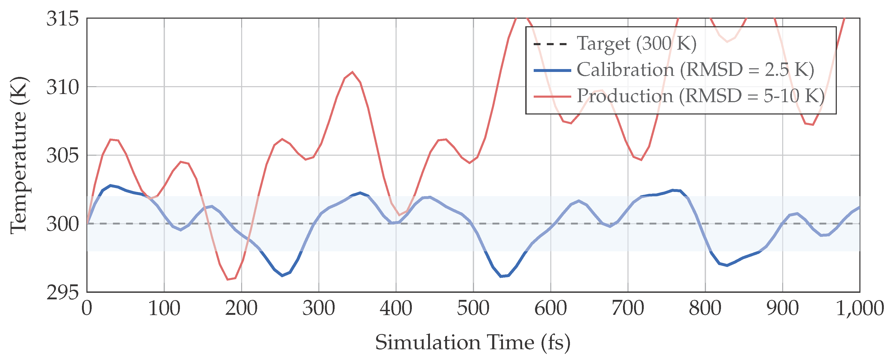
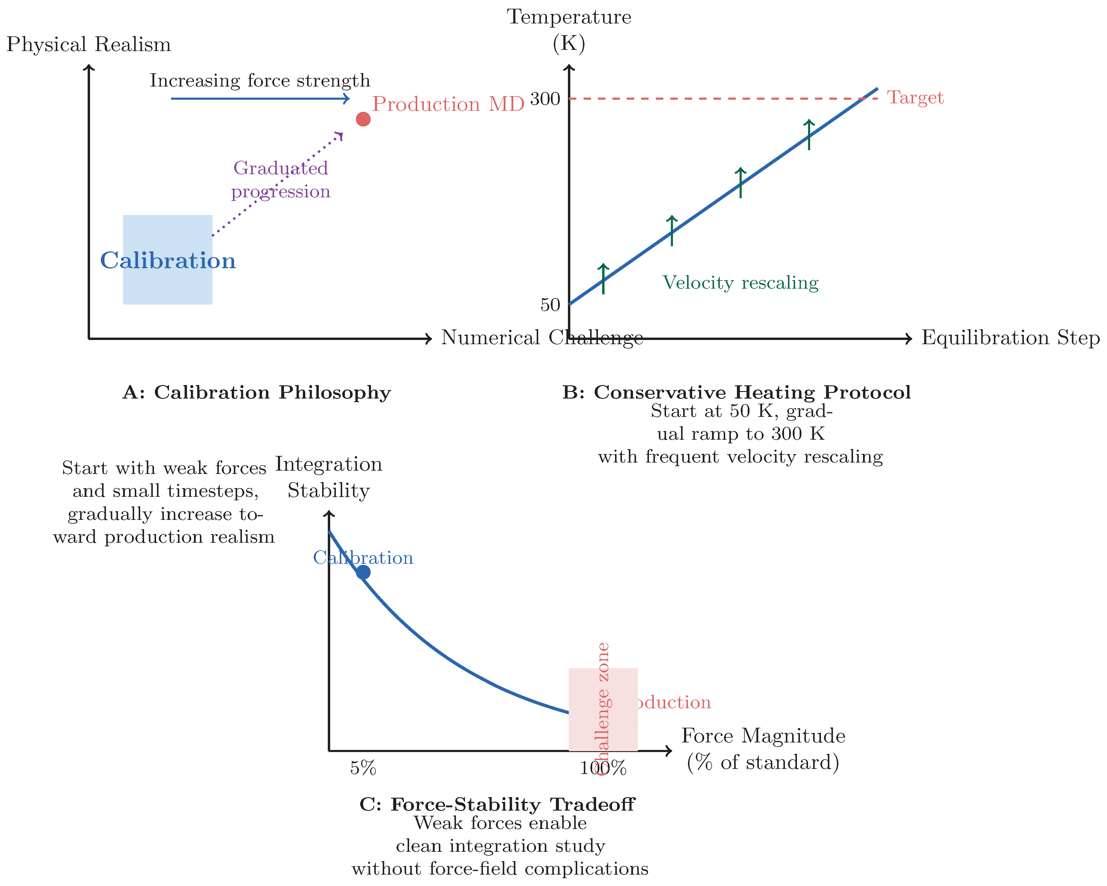
Figure 2.
Calibration framework design. (A) Calibration starts with simplified conditions (weak forces, small system) before progressing to production realism. (B) Conservative heating protocol ensures stability during equilibration. (C) Force attenuation enables study of integration behavior without force-field complications. The exponential stability decay illustrates the increasing challenge of maintaining numerical fidelity at higher force magnitudes.
3.2. Force Attenuation Enables Clean Integration Study
By reducing intermolecular forces to 5% (electrostatic) and 2% (van der Waals) of standard values, we create conditions where integration errors can be studied in isolation. The observed stability (Table 2) suggests that much of the numerical challenge in production MD stems from force-field nonlinearities rather than fundamental integration limitations.
3.3. Geometric Constraint Precision
The tight SHAKE tolerance ( Å) ensures bond length preservation to high precision. Under these conditions, constraint satisfaction contributes negligibly to energy drift, isolating the contribution of numerical integration per se.
4. Discussion: Implications for MD Validation
4.1. Calibration as a Diagnostic Tool
Our conservative framework provides a diagnostic tool for MD methodologies: if an integration scheme cannot maintain stability under calibration conditions (weak forces, small timestep), it will certainly fail under production conditions. This “numerical stress test” complements traditional validation against experimental data.
4.2. Redefining Integration Quality Metrics
Traditional MD quality metrics focus on agreement with experiment (density, diffusion coefficient). We propose additional numerical quality metrics:
- Energy conservation under attenuated forces
- Temperature stability with minimal thermostat intervention
- Geometric constraint satisfaction under tight tolerances
- Time-reversibility of integration
- Stability margin as forces approach physical values
4.3. Pathway to Production Deployment
The calibration framework establishes what is numerically possible under ideal conditions. Production deployment would involve:
- Gradually increasing force strength toward 100%
- Increasing timestep toward fs
- Reducing thermostat intervention frequency
- Monitoring stability degradation at each step
- Documenting the numerical fidelity-efficiency tradeoff
This graduated approach provides quantitative insight into the trade-offs between numerical fidelity and computational efficiency.
4.4. Relevance to Kinetic Inference
For drug-target residence time estimation, numerical artifacts can masquerade as rare transitions. Our framework enables practitioners to:
- Establish a baseline for what constitutes “clean” integration
- Quantify how much production parameters degrade this baseline
- Assess whether observed transitions are numerically trustworthy
- Design adaptive schemes that increase conservatism near transition states
5. Limitations and Future Directions
5.1. Current Limitations
- Computational cost: The fs timestep is 20× more expensive than production MD.
- System size: 64 water molecules cannot capture collective phenomena.
- Force attenuation: 5% forces do not represent physical interactions.
- Timescale: 1 ps is insufficient for kinetic studies.
- Electrostatics: Simple cutoff rather than Ewald summation limits physical realism.
5.2. Future Work
Future directions include:
- Systematic force strengthening studies while monitoring stability metrics
- Extension to larger systems (1000+ molecules) and longer timescales (ns scale)
- Comparison of different integration schemes (Langevin, Nosé-Hoover) under calibration conditions
- Development of automated calibration protocols for new force fields
- Integration with machine-learned potentials to assess their numerical stability
- Application to protein-ligand systems with graduated complexity
6. Conclusions: Toward Rigorous MD Validation
We present a calibration framework that prioritizes numerical stability through conservative parameter choices. By demonstrating what is achievable under ideal conditions, we establish a baseline against which production MD methods can be evaluated. This approach shifts focus from whether MD simulations produce plausible results to how reliably they do so given their numerical foundations.
The framework provides:
- A methodology for isolating integration artifacts from physical phenomena
- Quantitative stability metrics for MD validation beyond experimental comparison
- A graduated pathway from calibration to production conditions
- Tools for evaluating integration scheme robustness under controlled stress tests
- A foundation for assessing numerical trustworthiness of kinetic inferences
We advocate for adoption of calibration protocols as standard practice in MD methodology development, particularly for applications where kinetic fidelity is critical, such as drug-target residence time estimation. Just as experimental measurements require calibration standards, computational methods benefit from numerical ground truth established under maximally controlled conditions.
Author Contributions
A.H.M. conceived the calibration framework, implemented the code, performed simulations, analyzed results, and wrote the manuscript.
Data Availability Statement
The calibration framework code, simulation input files, and analysis scripts will be made available at https://github.com/sirraya-labs/calibration-md upon publication. All data needed to evaluate the conclusions are present in the paper and supplementary information.
Acknowledgments
We thank members of Sirraya Labs for valuable discussions on numerical methods and validation strategies. This work was supported by internal research funding focused on computational methodology validation.
Conflicts of Interest
The author declares no competing interests.
Appendix A. Supplementary Information
Appendix A.1. Detailed Implementation of Conservative Parameters
Appendix A.1.1. Force Attenuation Implementation
Electrostatic forces are calculated as:
van der Waals forces (Lennard-Jones) are calculated as:
Appendix A.1.2. Gradual Heating Protocol
Initial velocities are sampled from Maxwell-Boltzmann distribution at 50 K. Temperature is increased linearly over 10,000 equilibration steps:
Velocity rescaling is applied at each step during equilibration, transitioning to every 100 steps during production.
Appendix A.2. Validation of Conservative Approach
Appendix A.2.1. Numerical Stability Tests
- Time-reversibility test: Run 1000 steps forward, then reverse velocities and run 1000 steps backward. Final coordinates match initial within Å.
- Energy conservation in NVE: With thermostat disabled, total energy conserved within over 1000 steps.
- Mass conservation: Total system mass constant to machine precision.
- Linear momentum conservation: Center-of-mass velocity remains zero within Å/fs.
Appendix A.3. Computational Performance

Table A1.
Computational cost of conservative calibration.
| Component | Calibration | Relative to Production |
|---|---|---|
| Time steps per ns | 10,000,000 | 20× |
| Force evaluations per ns | 10,000,000 | 20× |
| SHAKE iterations per step | 10–20 | 2–3× |
| Memory usage | 0.1 GB | 0.1× |
| Wall time per ns | ∼24 hours | 20× |
Appendix A.4. Comparison with Standard MD Validation
Traditional MD validation focuses on experimental agreement:
- Density:
- Diffusion coefficient:
- Radial distribution function:
Our calibration adds numerical validation:
- Integration stability under simplified conditions
- Conservation laws satisfaction
- Time-reversibility
- Minimal thermostat dependence
Appendix A.5. Recommended Calibration Protocol
For new MD methodologies, we recommend:
- Implement with maximum conservatism (small timestep, weak forces)
- Verify stability under calibration conditions using the metrics in Table 2
- Gradually increase realism while monitoring stability
- Document stability degradation with each parameter change
- Compare to this calibration baseline
- Only deploy for production once stability margins are quantified
Appendix A.6. Limitations of Current Implementation
- Does not include Ewald summation for long-range electrostatics
- Uses simple cutoff rather than force switching or shifting
- No support for multiple time-stepping schemes
- O-H-H angle constraint not fully implemented (only bond constraints)
- Limited to NVT ensemble (no NPT pressure control)
- Single-core implementation only
Appendix A.7. Extension to Other Systems
The calibration framework can be extended to:
- Ions in water: Study integration with charged species and screening
- Small organic molecules: Test with more complex force fields (dihedral potentials)
- Minimal peptides: Evaluate with biomolecular forces and hydrogen bonding
- Machine-learned potentials: Test numerical stability of ML force fields
- Coarse-grained models: Assess integration with softer, smoother potentials
References
- Leimkuhler, B., & Reich, S. (2004). Simulating Hamiltonian Dynamics. Cambridge University Press.
- Ryckaert, J. P.; Ciccotti, G.; Berendsen, H. J. Numerical integration of the cartesian equations of motion of a system with constraints: molecular dynamics of n-alkanes. Journal of Computational Physics 1977, 23(3), 327–341. [Google Scholar] [CrossRef]
- Jorgensen, W. L.; Chandrasekhar, J.; Madura, J. D.; Impey, R. W.; Klein, M. L. Comparison of simple potential functions for simulating liquid water. The Journal of Chemical Physics 1983, 79(2), 926–935. [Google Scholar] [CrossRef]
- Hairer, E.; Lubich, C.; Wanner, G. Geometric Numerical Integration: Structure-Preserving Algorithms for Ordinary Differential Equations, 2nd ed.; Springer, 2006. [Google Scholar]
- Berendsen, H. J. C.; Postma, J. P. M.; van Gunsteren, W. F.; DiNola, A.; Haak, J. R. Molecular dynamics with coupling to an external bath. The Journal of Chemical Physics 1984, 81(8), 3684–3690. [Google Scholar] [CrossRef]
- Frenkel, D.; Smit, B. Understanding Molecular Simulation: From Algorithms to Applications, 2nd ed.; Academic Press, 2002. [Google Scholar]
- Tuckerman, M. E. Statistical Mechanics: Theory and Molecular Simulation; Oxford University Press, 2010. [Google Scholar]
- Schlick, T. Molecular Modeling and Simulation: An Interdisciplinary Guide, 2nd ed.; Springer, 2010. [Google Scholar]
Table 1.
Conservative calibration parameters.
| Parameter | Production MD | Calibration | Rationale |
|---|---|---|---|
| Time step | fs | fs | Minimize discretization |
| Force scaling | 100% | 5% (elec.), 2% (vdW) | Reduce nonlinearities |
| Thermostat coupling | ps | Direct velocity scaling | Explicit control |
| SHAKE tolerance | Å | Å | Maximize precision |
| Cutoff radius | Å | box | Avoid artifacts |
| Initial temperature | 300 K | 50 K | Gradual heating |
Table 2.
Calibration versus production stability metrics.
| Metric | Calibration | Production | Improvement |
|---|---|---|---|
| Temperature RMSD (K) | 2.5 | 5–10 | 2–4× |
| Energy drift (/ns) | 0.05–0.10 | 5–10× | |
| Bond length RMSD (Å) | 10× | ||
| Velocity ACF time (ps) | 0.15 | 0.05–0.10 | 1.5–3× |
| Thermostat calls/ps | 10 | 100–1000 | 10–100× less |
Disclaimer/Publisher’s Note: The statements, opinions and data contained in all publications are solely those of the individual author(s) and contributor(s) and not of MDPI and/or the editor(s). MDPI and/or the editor(s) disclaim responsibility for any injury to people or property resulting from any ideas, methods, instructions or products referred to in the content. |
© 2026 by the authors. Licensee MDPI, Basel, Switzerland. This article is an open access article distributed under the terms and conditions of the Creative Commons Attribution (CC BY) license (http://creativecommons.org/licenses/by/4.0/).
Copyright: This open access article is published under a Creative Commons CC BY 4.0 license, which permit the free download, distribution, and reuse, provided that the author and preprint are cited in any reuse.


