Submitted:
06 January 2026
Posted:
07 January 2026
You are already at the latest version
Abstract
(1)The previous theoretical studies showed that the large-scale vorticity generate the divergent-type helicity flux from the magnetic fluctuations. Similarly to the $\alpha$ effect, this breaks the equatorial reflection symmetry of the magnetic fluctuations in the stellar convection zone. This effect was called the new Visniac flux (hereafter the NV flux). 2)Methods. Using the mean-field dynamo model we study the effect of the NV flux on the solar type dynamos. 3)Results. We found that the NV flux results to a increase of the dynamo efficiency for the turbulent generation of the large-scale poloidal magnetic field of the Sun. The dynamic effect of the NV flux on the magnetic field evolution results into concentrating the dynamo waves toward the equator. Using the numerical simulations of the mean-field dynamo model we compare the helicity production rates by the turbulent dynamo effects, like the $\alpha$ effect and the NV flux. The model shows that the new dynamo source due to large-scale vorticity and small-scale dynamo results into amplification of the poloidal magnetic field generation in polar regions at the top of dynamo domain. Therefore the fluctuating magnetic activity at high latitudes of the Sun provides the additional source of the large-scale poloidal magnetic field.
Keywords:
sun
; magnetic cycles
; dynamo
1. Introduction
The basic scenario of the solar dynamo was suggested by Parker [1,2]. It is employed in the mean-field dynamo models which simulate the large-scale dynamo as a cyclic transformation of the poloidal magnetic field to the toroidal by means of the differential rotation and regeneration of the poloidal magnetic field from the toroidal by means of the cyclonic turbulent convection, the effect, and the systematic tilt magnetic field inside bipolar solar active regions, i.e., the Joy’s law. The origin of the effect is related with the effect of the Coriolis force on the convection in the stratified rotating convection zone. The origin of the tilt of the bipolar active regions (hereafter, BMR) is still under debate. Both the effect and the systematic tilt of the BMR are due to the breaking of the reflectional symmetry of the turbulent motions and magnetic field inside the convection zone. It is noteworthy that the large-scale dynamo produces the helical large-scale magnetic field with the positive helicity in the northern and the negative one in the southern hemisphere. The conservation of the total magnetic helicity results into opposite hemispheric helicity rule for the small-scale magnetic field. The theoretical arguments of Pouquet et al. [3], Frisch et al. [4], Kleeorin and Ruzmaikin [5] showed that the obtained distribution of the small-scale magnetic helicity opposes the turbulent generation of the large-scale poloidal magnetic field in stellar convective zones.
The nonlinear feedback of the magnetic helicity on the turbulent dynamo gave a motivation to study the effects of the magnetic helicity transports to overcome the restrictions of the magnetic helicity conservations in the large-scale dynamo [6,7,8]. In particular, the results of Pipin [9], Kleeorin and Rogachevskii [10], Gopalakrishnan and Subramanian [11] (hereafter, P08, KR22, and GS23, respectively) showed that in the large-scale vorticity can generate the magnetic helicity even when the original turbulent motions and magnetic fields have no helicity at all. For this effect the small-scale magnetic fields that stem from the small-scale dynamo are essential. The small-scale dynamo is expected to exist in the turbulent media of the stellar convective envelopes [12]. In the stellar convection zone the large-scale vorticity corresponds to the presence of the differential rotation and the meridional circulation. Both types of the large-scale flow contribute to generation of the magnetic helicity flux which is accompanied to the magnetic activity on the solar surface. The differential rotation is considered as the main source of the magnetic helicity transport from the solar convection zone to the outer layers of the Sun [13,14,15]. The results of Prior and Yeates [16] and Pipin et al. [17] showed that the differential rotation can be the main source of the hemispheric helicity rule of the magnetic field in solar active regions.
Following the results of the analytical studies of Gopalakrishnan and Subramanian [11] (hereafter GS23) and results of the above mentioned numerical simulations we conclude that the differential rotation can be an important source of the small-scale magnetic helicity in the solar convection zones. Interesting that this source of the magnetic helicity is rarely included in the dynamo models. The results of Guerrero et al. [18] showed that the differential rotation can be important for the helicity flux. The so called Visniac-Cho flux [7] which they studied is nonlinear about the large-scale magnetic field. Therefore, it is likely important for the supercritical dynamo regimes. However, the results of P08, KR22 and GS23 showed that the large-scale vorticity produces the magnetic helicity even for the linear case about the strength of the large-scale magnetic field. This term should be dominant for a slightly overcritical dynamos. Here, we study this effect in the mean-field dynamo for the first time. Our plan is as follows. Next chapter formulates the dynamo model and the basic assumptions behind it. In the chapter 3 we consider the results of the dynamo model and compare the new effects of the helicity generation with the standard effects of the large-scale dynamo. Finally, in chapter 4, we discuss the findings and draw the main conclusions of the paper.
2. The Dynamo Model
The evolution of the large-scale magnetic field, , in the highly conductive turbulent media is governed by the induction equation,
where is the mean electromotive force of the turbulent flows and magnetic field; is the large-scale flow. Here, the angle brackets mark the averaging over the ensemble of fluctuations. Usually, see e.g., Pipin et al. [17] we distinguish the axisymmetric and nonaxisymmetric components of the magnetic field and flows:
where the overline marks the longitudinal average. In this paper, we study the axisymmetric mean-field dynamo and put , . In following the line of Krause and Rädler [19], the axisymmetric field is decomposed into the sum of the poloidal and toroidal parts:
where the scalars A, B and the angular velocity are the functions of time and spatial variables: r is the radius and is the co-latitude (the polar angle); is the unit vector along the azimuth; is the meridional circulation. The details of our model can be found in [20]. The dynamo model employs the mean electromotive force, , as follows,
where describes the turbulent generation by the hydrodynamic and magnetic helicity, is the turbulent pumping and - the eddy magnetic diffusivity tensor. The -effect tensor includes the effect of the magnetic helicity conservation [5,21],
Here is the dynamo parameter characterizing the magnitude of the hydrodynamic -effect, and and are dimensionless and describe the anisotropic properties of the kinetic and magnetic -effect. Their radial profiles depend on the equipartition parameter, , the mean density stratification and the spatial profiles of the convective velocity , and on the Coriolis number,
where is the global angular velocity of the star and , are the convective turnover time and the mixing length respectively. The magnetic quenching function depends on the parameter [22]. We put the description of and as well as turbulent pumping tensor, and the eddy magnetic diffusivity tensor, . in Appendix.
To calculate the reference profiles of mean thermodynamic parameters, such as entropy, density, temperature and the convective turnover time, , we use the MESA model [23,24]. We use the mixing-length approximation to define the profiles of the eddy heat conductivity, , eddy viscosity, , eddy diffusivity, , and the RMS convective velocity, , as follows,
where we take into account the smooth decrease of toward the bottom of the convection zone; here, we put . The dynamo domain is divided for two parts. The convection zone extends from to . The model employs the overshoot layer below the convection zone to describe the transition from the differential rotation of the convection zone to the rigid rotation in the radiative zone at the position . The given depth of the overshoot layer allows us to bring the parameters of the radial gradient of the angular velocity close to the helioseismology results. In the transition region the turbulent parameters are defined following the results of Ludwig et al. [25], also see Paxton et al. [23]. We apply an exponential decrease of all turbulent coefficients (except the eddy viscosity and eddy diffusivity) with decrement -100, i.e., they are multiplied by a factor of , where z is the distance from the bottom of the convection zone. The eddy viscosity and eddy diffusivity are kept finite at the bottom of the tachocline, i.e., for the eddy viscosity coefficient profile within the tachocline we put
where is the value at the bottom of the convection zone, is the value inside the tachocline, z is the distance from the bottom of the convection zone. We use in the model, and we do similarly for the magnetic eddy diffusivity. The angular velocity profile, , and the meridional circulation, , are defined by conservation of the angular momentum and azimuthal vorticity . In this paper we use the kinematic models excluding the magnetic feedback on the large-scale flow and heat transport. The model shows an agreement of the angular velocity profile with helioseismology results for . The dynamo models with local show cycle period of 22 years when and 2, see futher details in [22].
Figure 1 shows the profiles of the large-scale flows, the hydrodynamic effect and the diffusivity profiles. We note the inverse sign of the effect tensor components and the rotational quenching of the turbulent diffusivity profile toward the bottom of the convection zone which is marked by the dashed line. Figure 1d), e) and f) show streamlines of the effective drift velocity of large-scale magnetic field due to the turbulent pumping and the meridional circulation. We see that the effective drift patterns are different for the toroidal and poloidal magnetic fields. Also, it depends on the magnetic fluctuations via the equipartition parameter because of the diamagnetic pumping. These effects were extensively discussed in [26,27].
In the paper we employ the conservation of the total magnetic helicity [32,33], , where integration is done over the volume of the convection zone. The differential form of the conservation law is as follows
where is the turbulent flux of the magnetic helicity density, . In this equation, we neglect effects of the Ohmic diffusion of the small- and large-scale magnetic helicity, and the Ohmic diffusion of the large-scale current helicity. The Ohmic dissipation of the small-scale current helicity was approximated as follows [21] :
where we put . Following the results of Gopalakrishnan and Subramanian [11] (hereafter, GS2023) we take in the following form,
where is the Fickian flux by the turbulent diffusion of the magnetic helicity; the and stand for the random advection flux and the new Vishniac flux (NV), respectively. For GS2023 got
Calculations of GS2023 does not take into account the effect of the Coriolis force and the large-scale magnetic field on the helicity flux. Results of P08 and KR22 show a complicated structure of the helicity fluxes under effects of the global rotation and large-scale magnetic field. In this study we take into account the rotational and magnetic quenching of the transport effects in heuristic way, in following the results of P08 and using the same quenching functions as for the magnetic part of the alpha effect. These quenching functions are needed for the numerical stability of the model. Following to results of P08, the effects of the magnetic helicity generation in the rotating turbulence are subjected to the quenching by means of the Coriolis force. Since the diffusive flux, is proportional to the magnetic eddy diffusivity we apply the same rotational quenching functions as for the isotropic part of the eddy diffusivity tensor, i.e, we put
where we put and for compatibility with the results of Mitra et al. [34] we will use (the range 0.1-0.5 is employed in the dynamo model). Following to the results of GS23 we get for the random advection flux,,
where, ; also, in transforming the expression given by GS23 we put and . Using , we transform to
We do the same reduction for GS23’s flux. After such simplification we get
The constant in the last equation is and it is if we consider the results of KR22 (see, expression in their Eq(E6)). The free parameter measures the efficiency of the helicity production. In our reduction of the given by GS23 we neglect the combined term with the numerical factor which is two order of magnitude less than that given by Eq(21). For the numerical stability we include the algebraic quenching of the flux given by the same function as for the - effect.
The large-scale vorticity is computed from the angular velocity distribution. In the spherical coordinate system we have , where and is the global angular velocity of the star. We neglect the azimuthal part of the large-scale vorticity due to the meridional circulation. Figure 2 shows the distribution of the large-scale vorticity in the solar convection zone and the velocity of the small-scale helicity transport by . The latter is outward in the main part of the convection zone and it is inward near the bottom.
Both the flux and describe the magnetic helicity generation from the large-scale flow and the small-scale magnetic fluctuations due to turbulent dynamo. Hence they can produce the large-scale dynamo effect even if the kinetic effect is negligible. Also, we see that the large-scale vorticity affect the nonlinear balance of the helicity distributions in the radial and latitudinal directions.
The dynamo model employs the zero magnetic field boundary conditions at the bottom of the overshoot layer, , at the top we smoothly connect the dynamo solution with the outer harmonic magnetic field [35], that satisfies,
for the region and the radial magnetic field for . We use as suggested by the results of the above-cited paper. To connect the external magnetic field with the dynamo region we employ the continuity of the normal component of the magnetic field and the tangential component of mean electromotive force, i.e., we put
where is the surface value of the turbulent magnetic diffusivity and is the mean effective diffusivity in the stellar corona. The solar type dynamo can be obtained when 1, i.e, when the corona is close to the ideal insulator state. Following the results of Pipin et al. [17] we put . The numerical code employs the pseudo-spectral method of integration in latitude with 64 Legendre nodes from the North to the South poles. In the radius it utilizes the finite differences with 120 mesh points from the bottom of the dynamo domain to the top . The Table 1 contains the description of the runs which will be discussed in the next chapter. Each run was started from the weak poloidal field of the equally mixed parity and 1 G strength. The solution was followed until it reach the stationary stage. The models with have a higher dynamo threshold than the case .
3. Results
Figure 3 show the snapshots of the reference models M0 and M1 for the decaying phase of the magnetic cycle. We see that the reduction of the intensity of the magnetic fluctuations, i.e., results to a considerable change in the pattern of the dynamo activity. Firstly, the radial propagation of the dynamo waves is not seen in the case M1. Secondly, the activity of the toroidal filed is concentrated strongly toward the bottom of the convection zone. This effect result to a decrease of the magnitude of the toroidal magnetic field flux in the dynamo in the run M1 in compare to the run M0. The run M1 show the longer dynamo period than the run M0 because the toroidal magnetic field evolves in the region with low magnetic diffusivity. All these effects in the run M1 are mainly because of the diamagnetic pumping pumping which is not active in the case . The d) column in Figure 3 show variations of the total effect, and its magnetic part which is due to the small-scale magnetic helicity generation. The dynamic variations of the effect at low latitudes in the run M0 are greater than in the run M1.
Addition of the helicity generation due the large-scale vorticity results to a strong modification of the total effect both near the bottom and the top of the convection zone. Figure 4 shows the snapshots of the magnetic field distribution and helicity generation rate in the dynamo model for the decaying phase of the activity cycle. The runs show that in the main part of the convection zone the small-scale helicity generation rate by the source is an order of magnitude less than that by the standard effect. However the effects have same magnitudes near the bottom of the convection zone and near the surface in the polar regions of the star. The run M2 demonstrates the significant change of the total effect in these regions. The animations of constructed using the results of run M2 and M3 show significant variations of the effect in the magnetic cycle due to the new source of the magnetic helicity generation. Similarly to the case M1, the run M3 shows a decrease of the effect variations in the bulk of the convection zone in compare to the run M2. The increase of the total effect near the surface in the polar regions the run M2 in compare to run M0 results to a stronger magnitude of the magnetic cycle. Simultaneously, run M2 shows a wider region of the inverted effect at low latitudes near the bottom of the convection zone that the run M0. Following to the Parker-Yoshimura rule this amplifies the propagation of the dynamo wave in this region toward the equator and bottom-ward. This seems affect the period of the dynamo cycle in the bulk of the convection zone, see Table 1.
Similarly to the runs M0 and M1 a decrease the level of the magnetic fluctuations to results to the change of the dynamo wave propagation pattern and the increase of the toroidal magnetic field near the bottom of the convection zone and in overshoot layer. The latter results to a decrease of the effect modulation near the bottom of the convection zone. The run M3 shows smaller modulation of the effect near the top of the convection zone in compare to the run M2.
Figure 5 illustrates the increase of the dynamo efficiency in the run M2 in compare to the run M0 by the time-latitude diagrams of the large-scale magnetic field and small-scale magnetic helicity. In the northern hemisphere of the star the run M2 shows an increase generation of the positive small-scale magnetic helicity around 50° latitude during the decaying phase of the magnetic cycle when the radial magnetic field grows in the polar regions. The Table 1 shows the magnitude of the polar magnetic field in the run M2 is by factor two larger than in the run M0.
In this paper I discuss only a few runs with the purpose of illustration of the dynamo effects due to the large-scale vorticity and the fluctuating magnetic field that stem from the small-scale dynamo. Let’s discuss the the effect of the parameter variations. When the small-scale dynamo absent, 1, then the helicity transport by the turbulent motions stratification effects decrease by the factor of magnitude, see Figure 2c. The flux disappears in this case. The moderate reduction of the small-scale parameter , see the runs M1 and M3 results into decrease of the dynamo efficiency of the convective envelope. The decrease of results into increase of the critical dynamo threshold of the effect. We find the longer dynamo period with the increase of the turbulent diffusion flux. It results into reduction the magnetic cycles overlap, as well. The latter affect the extended mode of the torsional osculations [22]. We find that the new dynamo source due to can produce the large-scale dynamo even in the case when the kinetic effect is zero. We postpone discussion of this case as well as effect of the nonlinear helicity transport to a separate paper.
4. Discussion and Conclusions
In this paper we discussed the large-scale dynamo effects of the divergent helicity flux due to the large-scale vorticity and small-scale dynamo magnetic fluctuations. The magnetic helicity flux is usually considered as a solution of the so-called -effect catastrophic quenching [36]. In this case the helicity generation follows conservation of the total magnetic helicity in the large-scale dynamo as a response for generation large-scale magnetic field by the kinetic effect. Results of Kleeorin et al. [6], Vishniac and Cho [7], Field and Blackman [37] showed the catastrophic quenching can be alleviated if the magnetic helicity transport by the turbulent motions is taken into account. Generation of the small-scale magnetic helicity in the dynamos is a nonlinear about the - field effect. The analytical results of Kleeorin and Rogachevskii [10], Subramanian and Brandenburg [38] showed that the small-scale helicity can be generated by the large-scale vorticity and the chaotic small-scale magnetic field that stem from the small-scale dynamo. Generation of the preferred hemispheric helicity from the random magnetic field distribution by the differential rotation is known for a long time, see e.g., Berger and Ruzmaikin [13], Pariat et al. [14], Berger [39]. The results of the numerical model show that the differential rotation can generate the negative helicity in the near equatorial regions at the northern hemisphere and positive at the southern [16,17]. The opposite pattern is generated at high latitudes. The generated magnetic helicity participates in the dynamo process and it must be taken into account. The results of KR22 and GS23 formulate this effect in a general analytical form. Here, for the first time we consider this effect for the solar type dynamos. The new dynamo source in the studied dynamo model ss constructed in heuristic way because we do not know the impact of the Coriolis force and the large-scale magnetic field on . This affect all our conclusions constructed on the base of the presented runs.
The results of our runs shows that the new source of the magnetic helicity modifies the patterns of the dynamo waves propagation inside the convection zone, increases the amplitude and the dynamo period. These changes are caused by modification of the effect. The source is concentrated toward the boundaries of the convection zone because of variation of the differential rotation, the convective turnover time and the mean density stratification. These factors results to a modulation of the effect near the boundaries. Near the bottom the source increases the inversion of the effect. In following the Parker-Yoshimura rule [40], the negative ( in the northern hemisphere) and the positive gradient of the angular velocity result into amplification of the equatorward dynamo waves in equatorial regions near the bottom of the convection zone. Simultaneously the negative shear in the polar regions together with the negative gradient of the mean density and the small-scale dynamo magnetic field amplify generation of the poloidal magnetic field near the surface in the polar regions of the star. The latter means that the polar magnetic field can be regenerated in-situ if there is the toroidal magnetic field there. Therefore the large-scale vorticity amplifies the action of the kinetic -effect in the polar regions of the star. Similarly to the dynamo, see Kitchatinov and Olemskoy [41], the new dynamo source is likely to be important for the fast rotating stars that have the finite amplitude of the differential rotation.
Let us summarize our findings. Using the mean-field dynamo model we study the effects of the large-scale vorticity and the magnetic fluctuations on the large-scale dynamo. The intensity of the magnetic fluctuations is given by the equipartition parameter . Its effect on the small-scale helicity production was estimated earlier in analytical studies of Pipin [9], Kleeorin and Rogachevskii [10], Gopalakrishnan and Subramanian [11] using the mean-field MHD framework. Our dynamo models show a crucial role of the magnetic helicity production via the large-scale vorticity in the large-scale dynamo process. It affects the magnetic field generation near the boundaries of the dynamo domain because of the strong variation of the mean turbulent parameters in these regions. We hope that the future study will clarify the nonlinear impact of the global rotation and magnetic fields on the level of the magnetic helicity production by the differential rotation and the magnetic fluctuations. References
Data Availability Statement
The data of the models are available by request from the author.
Acknowledgments
The author thanks the Ministry of Science and Higher Education of the Russian Federation for financial support (the project No.0278-2026-0001)
Conflicts of Interest
The authors declare no conflicts of interest.
Appendix A
The α effect.
In following to Pipin [9] (hereafter P08) we have
and
where the functions , define the Coriolis number dependence and dependence of the alpha effect tensors on the relative intensity of the magnetic fluctuations that stems from the small-scale dynamo. The latter is important for the NV helicity flux (see, GS2023). In the previous studies we simply use . Here we consider this as another parameter of the dynamo model. We put all the quenching functions in Appendix. The stratification scales parameters are and . It is worth to note that for the nearly adiabatic stratification of the stellar convection zone we have , where is the adiabatic index and is the mixing-length parameter we use and , is the mean pressure profile. The changes from about in the main part of the convection zone and it goes to below near the bottom. Therefore, the inverses the sign near the bottom of the convection zone. Functions were defined by Pipin [9], , and nHz.
The magnetic quenching function of the hydrodynamical part of -effect:
where
The turbulent pumping and eddy magnetic diffusivity.
In the model we take into account the mean drift of large-scale field due to the magnetic buoyancy, , the gradient of the mean density, and the diamagnetic pumping because of the turbulent intensity stratification, :
where the magnetic buoyancy modulation function reads
From Eq(25), we see that that when . In other words, the diamagnetic pumping disappears when the energy of the small-scale magnetic fluctuations is in equipartition with the energy of the convective flows.
We employ the anisotropic diffusion tensor following the formulation of P08 ignoring the generation effects from the large-scale current :
where is
References
- Parker, E.N. The Formation of Sunspots from the Solar Toroidal Field. Astrophys. J. 1955, 121, 491. [CrossRef]
- Parker, E. Hydromagnetic Dynamo Models. Astrophys. J. 1955, 122, 293–314.
- Pouquet, A.; Frisch, U.; Léorat, J. Strong MHD helical turbulence and the nonlinear dynamo effect. J. Fluid Mech. 1975, 68, 769–778.
- Frisch, U.; Pouquet, A.; Léorat, J.; A., M. Possibility of an inverse cascade of magnetic helicity in magnetohydrodynamic turbulence. J. Fluid Mech. 1975, 68, 769–778.
- Kleeorin, N.I.; Ruzmaikin, A.A. Dynamics of the average turbulent helicity in a magnetic field. Magnetohydrodynamics 1982, 18, 116–122.
- Kleeorin, N.; Moss, D.; Rogachevskii, I.; Sokoloff, D. Helicity balance and steady-state strength of the dynamo generated galactic magnetic field. Astron. Astrophys. 2000, 361, L5–L8, [arXiv:astro-ph/0205266].
- Vishniac, E.T.; Cho, J. Magnetic Helicity Conservation and Astrophysical Dynamos. Astrophys. J. 2001, 550, 752–760.
- Brandenburg, A.; Vishniac, E.T. Magnetic Helicity Fluxes in Dynamos from Rotating Inhomogeneous Turbulence. Astrophys. J. 2025, 984, 78, [arXiv:physics.plasm-ph/2412.17402]. [CrossRef]
- Pipin, V.V. The mean electro-motive force and current helicity under the influence of rotation, magnetic field and shear. Geophysical and Astrophysical Fluid Dynamics 2008, 102, 21–49, [arXiv:astro-ph/0606265].
- Kleeorin, N.; Rogachevskii, I. Turbulent magnetic helicity fluxes in solar convective zone. Mon. Not. R. Astron. Soc. 2022, 515, 5437–5448, [arXiv:astro-ph.SR/2206.14152]. [CrossRef]
- Gopalakrishnan, K.; Subramanian, K. Magnetic Helicity Fluxes from Triple Correlators. Astrophys. J. 2023, 943, 66, [arXiv:astro-ph.GA/2209.14810]. [CrossRef]
- Käpylä, P.J.; Browning, M.K.; Brun, A.S.; Guerrero, G.; Warnecke, J. Simulations of Solar and Stellar Dynamos and Their Theoretical Interpretation. Space Sci. Rev. 2023, 219, 58, [arXiv:astro-ph.SR/2305.16790]. [CrossRef]
- Berger, M.A.; Ruzmaikin, A. Rate of helicity production by solar rotation. J. Geophys. Res. 2000, 105, 10481–10490. [CrossRef]
- Pariat, E.; Démoulin, P.; Berger, M.A. Photospheric flux density of magnetic helicity. Astron. Astrophys. 2005, 439, 1191–1203. [CrossRef]
- Sun, Z.; Li, T.; Wang, Q.; Yang, S.; Zhang, M.; Chen, Y. Magnetic helicity evolution during active region emergence and subsequent flare productivity. Astron. Astrophys. 2024, 686, A148, [arXiv:astro-ph.SR/2403.18354]. [CrossRef]
- Prior, C.; Yeates, A.R. On the Helicity of Open Magnetic Fields. Astrophys. J. 2014, 787, 100, [arXiv:astro-ph.SR/1404.3897]. [CrossRef]
- Pipin, V.V.; Yang, S.; Kosovichev, A.G. Helicity Fluxes and Hemispheric Helicity Rule of Active Regions Emerging from the Convection Zone Dynamo. Astrophys. J. 2025, 991, 88, [arXiv:astro-ph.SR/2508.00309]. [CrossRef]
- Guerrero, G.; Chatterjee, P.; Brandenburg, A. Shear-driven and diffusive helicity fluxes in αΩ dynamos. MNRAS 2010, 409, 1619–1630, [arXiv:astro-ph.SR/1005.4818]. [CrossRef]
- Krause, F.; Rädler, K.H. Mean-Field Magnetohydrodynamics and Dynamo Theory; Berlin: Akademie-Verlag, 1980; p. 271.
- Pipin, V.V.; Kosovichev, A.G.; Tomin, V.E. Effects of Emerging Bipolar Magnetic Regions in Mean-field Dynamo Model of Solar Cycles 23 and 24. Astrophys. J. 2023, 949, 7, [arXiv:astro-ph.SR/2210.08764]. [CrossRef]
- Kleeorin, N.; Rogachevskii, I. Magnetic helicity tensor for an anisotropic turbulence. Phys. Rev.E 1999, 59, 6724–6729.
- Pipin, V.V.; Kosovichev, A.G. On the Origin of Solar Torsional Oscillations and Extended Solar Cycle. Astrophys. J. 2019, 887, 215. [CrossRef]
- Paxton, B.; Bildsten, L.; Dotter, A.; Herwig, F.; Lesaffre, P.; Timmes, F. Modules for Experiments in Stellar Astrophysics (MESA). Astrophys. J. Suppl. 2011, 192, 3, [arXiv:astro-ph.SR/1009.1622]. [CrossRef]
- Paxton, B.; Cantiello, M.; Arras, P.; Bildsten, L.; Brown, E.F.; Dotter, A.; Mankovich, C.; Montgomery, M.H.; Stello, D.; Timmes, F.X.; et al. Modules for Experiments in Stellar Astrophysics (MESA): Planets, Oscillations, Rotation, and Massive Stars. Astrophys. J. Suppl. 2013, 208, 4, [arXiv:astro-ph.SR/1301.0319]. [CrossRef]
- Ludwig, H.G.; Freytag, B.; Steffen, M. A calibration of the mixing-length for solar-type stars based on hydrodynamical simulations. I. Methodical aspects and results for solar metallicity. Astron. Astrophys. 1999, 346, 111–124, [astro-ph/9811179].
- Krivodubskij, V.N. Transfer of the large-scale solar magnetic field by inhomogeneity of the material density in the convective zone. Soviet Astronomy Letters 1987, 13, 338.
- Kitchatinov, L.L. Turbulent transport of magnetic fields in a highly conducting rotating fluid and the solar cycle. Astron. Astrophys. 1991, 243, 483–491.
- Harris, C.R.; Millman, K.J.; van der Walt, S.J.; Gommers, R.; Virtanen, P.; Cournapeau, D.; Wieser, E.; Taylor, J.; Berg, S.; Smith, N.J.; et al. Array programming with NumPy. Nature 2020, 585, 357–362. [CrossRef]
- Virtanen, P.; Gommers, R.; Oliphant, T.E.; Haberland, M.; Reddy, T.; Cournapeau, D.; Burovski, E.; Peterson, P.; Weckesser, W.; Bright, J.; et al. SciPy 1.0: Fundamental Algorithms for Scientific Computing in Python. Nature Methods 2020, 17, 261–272. [CrossRef]
- Hunter, J.D. Matplotlib: A 2D graphics environment. Computing in Science & Engineering 2007, 9, 90–95. [CrossRef]
- Sullivan, C.B.; Kaszynski, A. PyVista: 3D plotting and mesh analysis through a streamlined interface for the Visualization Toolkit (VTK). Journal of Open Source Software 2019, 4, 1450. [CrossRef]
- Hubbard, A.; Brandenburg, A. Catastrophic Quenching in αΩ Dynamos Revisited. Astrophys. J. 2012, 748, 51, [arXiv:astro-ph.SR/1107.0238]. [CrossRef]
- Pipin, V.V.; Sokoloff, D.D.; Zhang, H.; Kuzanyan, K.M. Helicity Conservation in Nonlinear Mean-field Solar Dynamo. Astrophys. J. 2013, 768, 46, [arXiv:astro-ph.SR/1211.2420]. [CrossRef]
- Mitra, D.; Candelaresi, S.; Chatterjee, P.; Tavakol, R.; Brandenburg, A. Equatorial magnetic helicity flux in simulations with different gauges. Astronomische Nachrichten 2010, 331, 130, [arXiv:astro-ph.SR/0911.0969]. [CrossRef]
- Bonanno, A. Stellar Dynamo Models with Prominent Surface Toroidal Fields. Astrophys. J. Lett. 2016, 833, L22, [arXiv:astro-ph.SR/1612.00253]. [CrossRef]
- Vainshtein, S.I.; Cattaneo, F. Nonlinear restrictions on dynamo action. Astrophys. J. 1992, 393, 165–171. [CrossRef]
- Field, G.B.; Blackman, E.G. Dynamical Quenching of the α2 Dynamo. Astrophys. J. 2002, 572, 685–692, [arXiv:astro-ph/0111470]. [CrossRef]
- Subramanian, K.; Brandenburg, A. Nonlinear current helicity fluxes in turbulent dynamos and alpha quenching. Phys. Rev. Lett. 2004, 93, 205001.
- Berger, Mitchell A.; Field, G.B. The topological properties of magnetic helicity. Journal of Fluid Mechanics 1984, 147. [CrossRef]
- Yoshimura, H. Solar-cycle dynamo wave propagation. Astrophys. J. 1975, 201, 740–748. [CrossRef]
- Kitchatinov, L.L.; Olemskoy, S.V. Differential rotation of main-sequence dwarfs and its dynamo efficiency. MNRAS 2011, 411, 1059–1066, [arXiv:astro-ph.SR/1009.3734]. [CrossRef]
Figure 1.
a) The meridional circulation (streamlines) and the angular velocity distributions; the magnitude of circulation velocity is of 13 m/s on the surface at the latitude of 45°; b) the -effect tensor distributions at the latitude of 45°, the dash line shows the convection zone boundary; b) radial dependencies of the total, , and the rotational induced part, , of the eddy magnetic diffusivity, the eddy viscosity profile, ; d) streamlines of the effective drift velocity of large-scale toroidal magnetic field due to the turbulent pumping and the meridional circulation for the case of equipartition between the intensity of the magnetic fluctuations and turbulent motions, ; e) the same as d) when the energy of the magnetic fluctuations is less by factor two than the energy of turbulent flows; f) streamlines of the effective drift velocity of large-scale poloidal magnetic field. We use numpy/scipy [28,29] together with matplotlib [30] and pyvista [31] for post-processing and visualization.
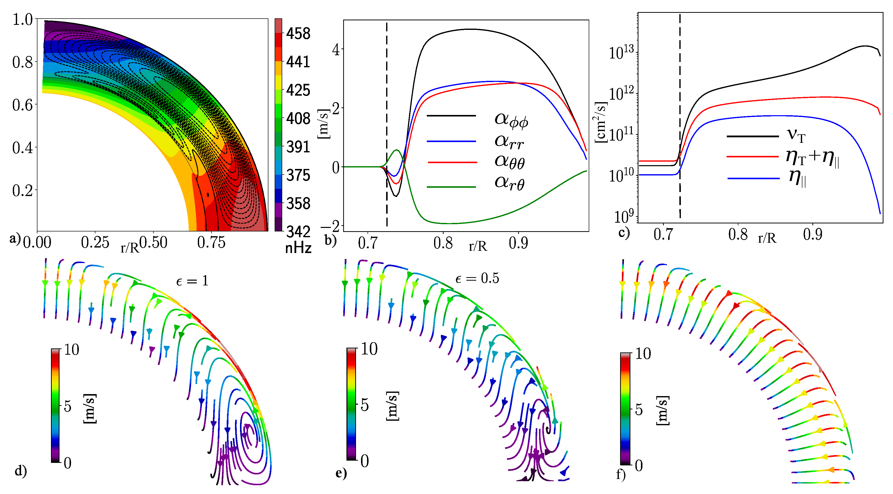
Figure 2.
Panels a) and b) show the components large-scale vorticity as due to the differential rotation of the Sun. It is noteworthy that and are antisymmetric and symmetric about the equator, respectively; c) the small-scale helicity transport velocity by .
Figure 2.
Panels a) and b) show the components large-scale vorticity as due to the differential rotation of the Sun. It is noteworthy that and are antisymmetric and symmetric about the equator, respectively; c) the small-scale helicity transport velocity by .
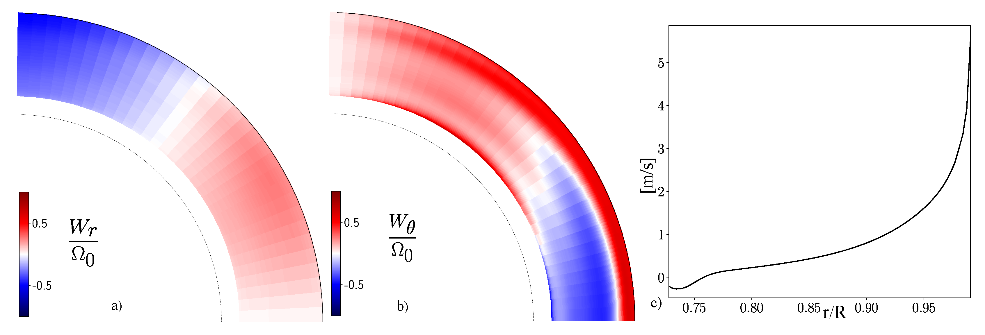
Figure 3.
Snapshots of the models M0 and M1 for the decaying phase of the magnetic cycle: a) the large-scale magnetic field distribution, color image shows the toroidal magnetic field and the streamlines show the poloidal magnetic field; b) the small-scale magnetic helicity density generation rate by the large-scale dynamo ; c) the same as b) for the effect contribution; d) the radial profiles of the effect, shows the contribution of the small-scale magnetic helicity.
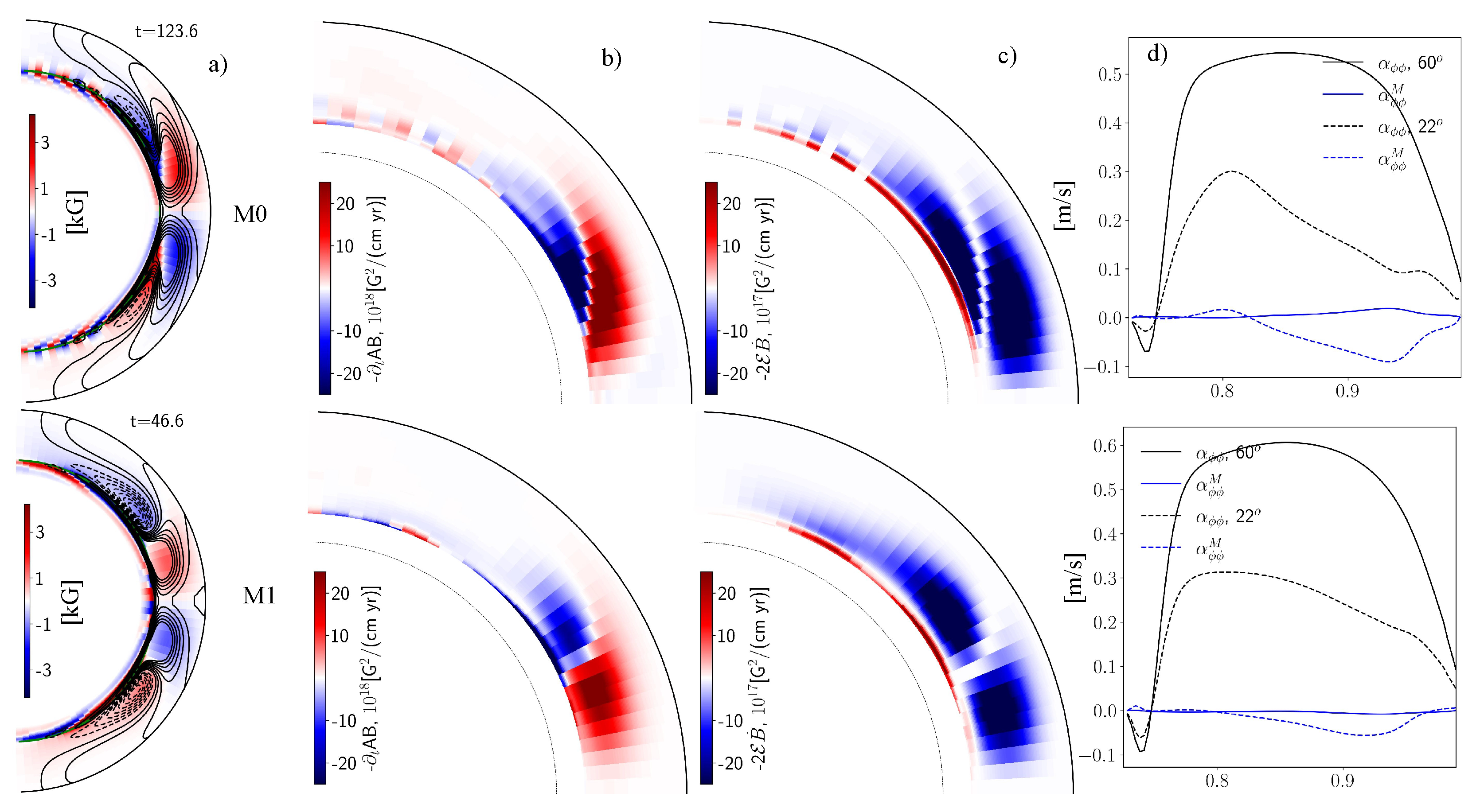
Figure 4.
The same as Figure 3 for the models M2 and M3. Here, the column d) show the new Vishniac flux contribution, . Note the substantial changes of the alpha effect near the bottom of the convection zone and at high latitude near the surface. Animations of this figure show variations of the magnetic field and the helicity generation rate distributions, as well as variations of the effect profiles during 3 magnetic cycles of the runs M2 and M3.
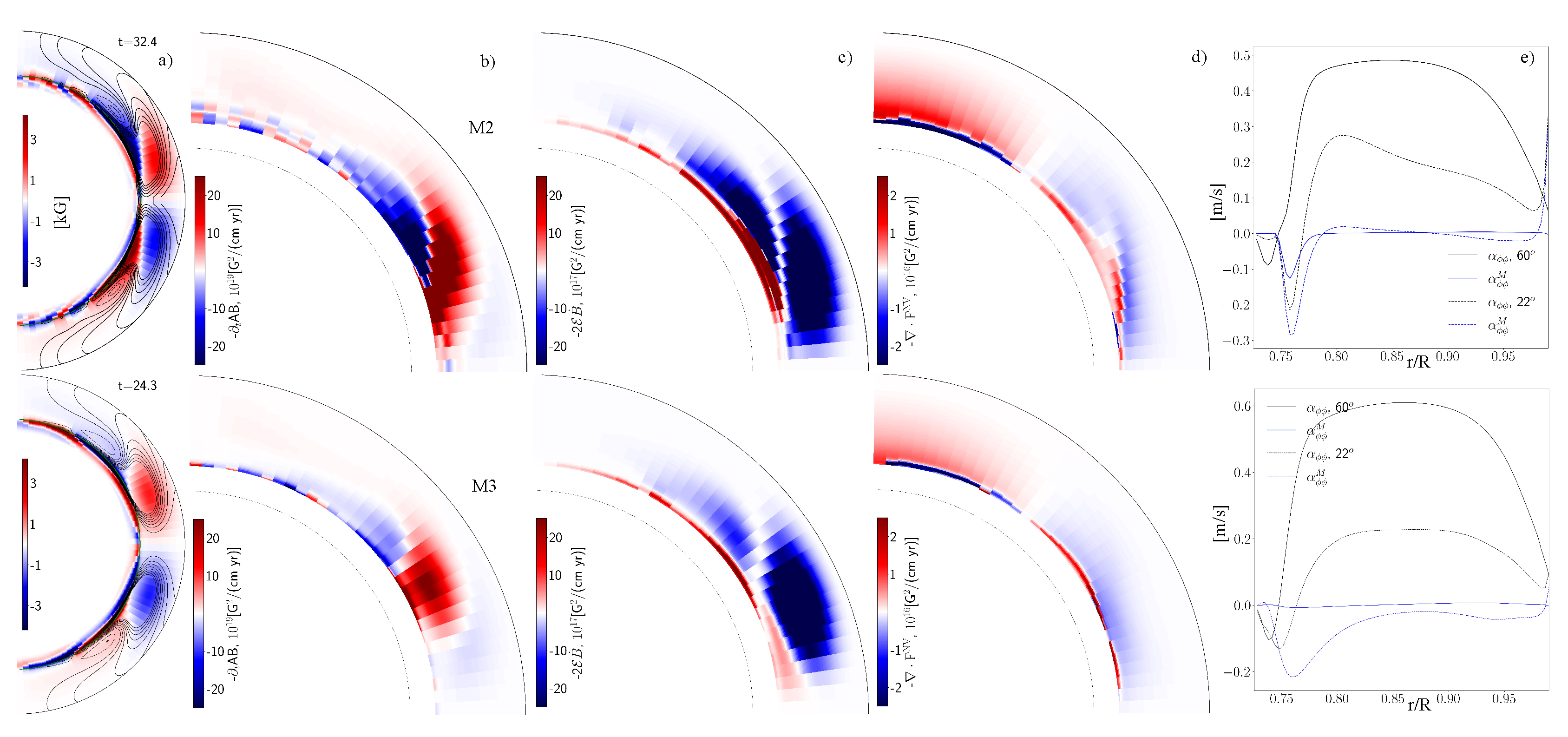
Figure 5.
a) The time latitude diagrams of the large-scale magnetic field in the model M0, contours show the toroidal magnetic field at ; b) the time latitude diagram of the small-scale helicity density evolution at the surface; c) and d) show the same for the run M2.
Figure 5.
a) The time latitude diagrams of the large-scale magnetic field in the model M0, contours show the toroidal magnetic field at ; b) the time latitude diagram of the small-scale helicity density evolution at the surface; c) and d) show the same for the run M2.
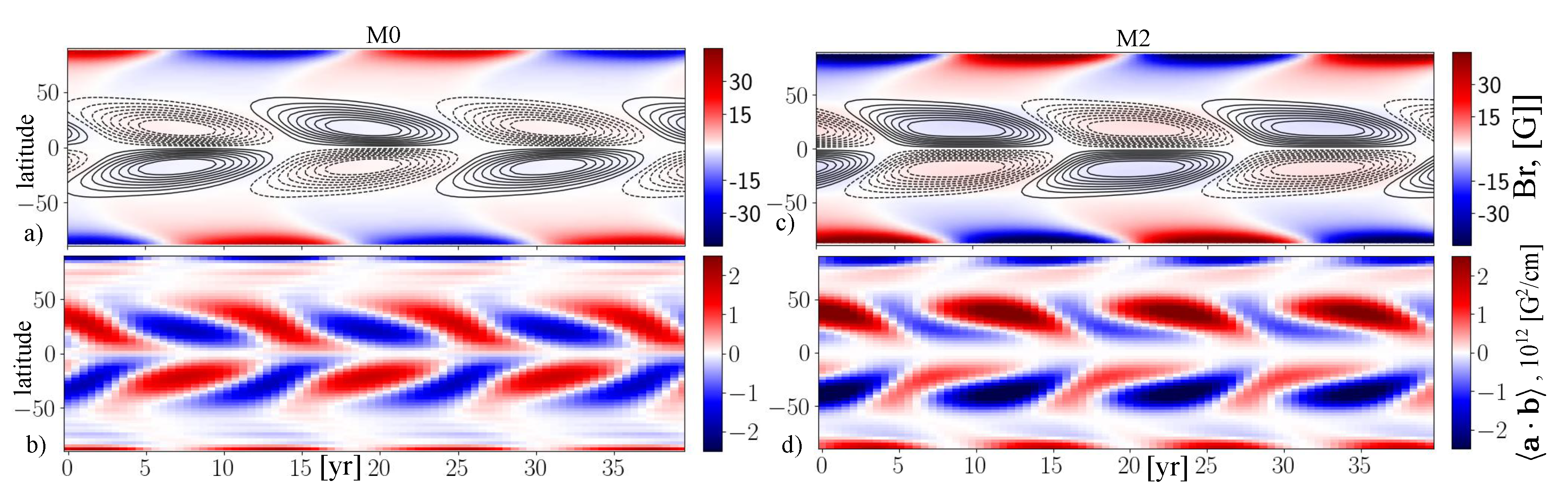

Table 1.
The models and parameters. Here, marks the magnitude and the total unsigned of the toroidal magnetic field in the dynamo region; shows the strength of the polar magnetic field at the surface; is the full magnetic cycle period; the Parity parameter shows the type of the equatorial symmetry of the magnetic fields, where D stands for the dipole-type symmetry magnetic field, Q stands for the quadrupole-type and D+ wQ is mix of the dipole type symmetry with a weak quadrupole-type symmetry, respectively.
| Model | [kG] | [Mx] | ,[G] | ,[yr] | Parity | |||||
|---|---|---|---|---|---|---|---|---|---|---|
| M0 | 0.045 | 1 | 0 | 0 | 0.1 | 4.1 | 1.45 | 30 | 20.8 | D |
| M1 | 0.055 | 0.5 | 0 | 0 | 0.1 | 8.1 | 1.25 | 53 | 26.5 | D+ w Q |
| M2 | 0.045 | 1 | 1 | 1 | 0.3 | 5.8 | 2.1 | 60 | 23.4 | D+ w Q |
| M3 | 0.055 | 0.5 | 1 | 1 | 0.3 | 8.3 | 1.02 | 58 | 24.5 | D+ w Q |
Disclaimer/Publisher’s Note: The statements, opinions and data contained in all publications are solely those of the individual author(s) and contributor(s) and not of MDPI and/or the editor(s). MDPI and/or the editor(s) disclaim responsibility for any injury to people or property resulting from any ideas, methods, instructions or products referred to in the content. |
© 2026 by the authors. Licensee MDPI, Basel, Switzerland. This article is an open access article distributed under the terms and conditions of the Creative Commons Attribution (CC BY) license (http://creativecommons.org/licenses/by/4.0/).
Copyright: This open access article is published under a Creative Commons CC BY 4.0 license, which permit the free download, distribution, and reuse, provided that the author and preprint are cited in any reuse.


