Submitted:
05 January 2026
Posted:
06 January 2026
You are already at the latest version
Abstract
Background: Impact wrenches are widely used in construction and automotive industries, yet they generate harmful vibrations that pose health risks to operators and reduce tool usability. Methods: A practical, low-order bond graph model of impact-wrench dynamics is developed, capturing interactions among the motor, hammer, anvil, and hand/arm constraints. The model is validated against measurements during bolt setting in a steel plate. Results: Predictions match measured RMS accelerations and spectral modes up to 200 Hz with errors within 11%. Analysis attributes the dominant vibration sources to rotational and translational impacts between the hammer and anvil; notably, the translational (z-axis) impact contributes substantially to felt vibration while not being required for bolt tightening. Conclusions: The model provides physical insight into vibration origins and supports actionable design decisions (e.g., eliminating the linear impact, adding rotational damping/control) consistent with ISO 28927-13:2022 testing practice.
Keywords:
impact wrench
; bond graph
; power tool
; hand–arm vibration
; vibration mitigation
; system dynamics
; mechatronics
; electromechanical systems
1. Introduction
The impact wrench (driver) is used in construction, automotive, and many other industries to tighten bolts. These devices are required to achieve higher torque and speed than with hand tightening. The functioning of an impact hammer is described by Matthiesen et al. [1]. The impacts that this tool generates repeat at approximately 42 Hz. These vibrations pose serious health risks to operators of such power tools. A public health practice paper [2] outlines the clinical signs of hand-arm vibrations (HAV) syndrome: blanched fingers, tenderness or pain and swelling of the fingers and forearm tissue, paresthesia or tingling in fingers, cold intolerance, weakness of the finger flexors or intrinsic muscles, loss of muscle control, reduced sensitivity to heat and cold, discoloration and trophic skin lesions of the fingers, and loss of manipulative dexterity and finger coordination. A study by Per Vihlborg et al. [3] found an association between vibration exposure and HAV symptoms (HAVs) in the Swedish mechanical industry. Workers exposed to HAV have a 4–5 fold increased risk of vascular and neurological diseases [4]. Animal models have been used to replicate the damage caused by HAVs [5]: in a field survey it was found that 15% of power tools exceeded the action limits according to applicable standards [6]. Mazaheri et al. [7] show that the industry still needs to develop stricter standards for vibration limits. There is significant evidence that the manufacturers’ declared vibration values are underestimated [8]. Recent exposure and dose–response studies further motivate reducing HAV in practice [9,10]. Most papers provide methods for assessing the exposure of vibrations produced by power tools or modeling of the hand–arm vibrations. This paper develops and validates a low-order model for illustrating the major contributing components of vibrations of impact hammers. Prior work has used finite element models to estimate impact coefficients [11]. Here, comparable results are obtained using bond graphs. This work differs from other studies and solutions in that it provides a low-order model for assessing the origins of hand–arm vibrations. This model can be used to test the relative efficacy of vibration control concepts. The bond graphs provide a level of abstraction that yields an understanding of the fundamental architecture of the system. This abstraction helps find and test possible solutions. The model was validated using the procedure shown in Figure 1.
Related Work and Contribution. Beyond finite-element approaches for impact modeling [11], a large body of work on biodynamic models of the human hand–arm system exists [12]. System-level identification of electric impact wrenches has also been explored [13]. In contrast to high-order FE, physiological, or ID-only models, the proposed physics-based low-order model targets rapid, system-level design exploration of the impact wrench as an electromechanical system, reproducing axis-wise RMS and spectral characteristics relevant to ISO 28927-13 while remaining simple enough to guide mechanism-level changes.
2. Model Development
Bond graphs were used to develop component models and then assemble the component models into an overall system model. Bond graphs are a pictorial representation of all types of dynamic systems interacting in multiple energy domains. Ref. [14] describes bond graph modeling and development. All the bodies are assumed rigid and contacts are represented by a linear stiff spring and damper. The model is limited to systems with similar dimensions and power. Figure 2 shows the tool mass, , the battery mass, , the total mass, , vertical distance from tool centerline to center of gravity (CG), , vertical distance from CG to battery, , vertical distance from CG to grip location, , horizontal distance from CG to grip location, , horizontal distance from tool tip to CG, . The sensor is located by vertical and horizontal distances from the CG. These can vary based on the location of the sensor.
Assumptions and Limitations. The tool is modeled as an assembly of rigid bodies with impacts represented by linear spring–damper contact elements. Small angular motions are assumed for the rigid-body coupling in Figure 4. Hand/arm interaction is represented using lumped linear translational and torsional constraints tuned to the literature, rather than a detailed physiological (distributed) model. As such, the model is intended for rapid, system-level design exploration and does not capture detailed structural flexibility, high-frequency modes beyond the validated range, or tooth-level contact mechanics.
Figure 3 shows the dynamic components of the impact hammer. The battery-powered electric motor of mass, , and moment of inertia, , drives the rotating shaft at angular velocity through a reduction gearbox of ratio, . The shaft has a slot at its end with a trapped ball that rotates the hammer of mass, , and rotational inertia, . The hammer then strikes the anvil of mass, , and rotational inertia, , such that the rotation of the hammer is virtually stopped. When this happens, the shaft continues to rotate and the ball-and-slot mechanism lifts the hammer until the hammer clears the anvil and rotates again. The ball/slot has a prescribed angle relative to the shaft and is represented here as a modulus, , specifying the rise of the hammer per rotation angle of the shaft. As the hammer is lifted, it compresses the spring of stiffness, and damping, , and then when the hammer clears the anvil the spring pushes the hammer back towards the anvil. The hammer continues to rotate and move downward until it strikes the anvil at a location 180 from the initial strike. As a result of the strike from the hammer onto the anvil, the anvil advances in the direction of the strike by some number of degrees depending on the load on the anvil. This is the basic operation of the impact hammer.
The impact between the hammer and anvil is a major source of vibration felt by an operator of the tool. Additionally, the compression and extension of the hammer spring also provides significant forcing on the tool. Ideally, the downward motion of the hammer after it clears the anvil would have the hammer reach the ’floor’ of the hammer just as it strikes the anvil the next time. In reality this rarely happens and the hammer can either impact the hammer floor prior to striking the anvil thus producing more unwanted vibration or it can miss the next strike completely by not being lowered sufficiently quickly during some part of the operating cycle. All of these potential scenarios are part of the dynamic model being developed here.
Impact between moving dynamic elements has been a research topic for many years. The work in [11] is indicative of the history of impact models. For the model here, impact is represented by a very stiff spring and damper, and , that are activated when the relative displacement between the impacting bodies is less than a specified amount. Related torsional-impact modeling and stiffness estimation for impact wrenches further supports this formulation [15], as do studies of energy/torque exchange during tightening [16]. The stiffness is determined through numerical experimentation and considered stiff enough when the displacement across the impact spring is less than a fraction of a millimeter. In this development, impact between the hammer and anvil, and between the hammer and ”floor” are both included.
Figure 4 is a bond graph fragment for the rigid body dynamics of the tool as a whole. Body-fixed coordinates are used as indicated in Figure 2. Gyroscopic coupling of the coordinates is considered, and small angular motions are assumed.
Figure 4.
Bond graph fragment of the rigid body dynamics using body fixed coordinates.
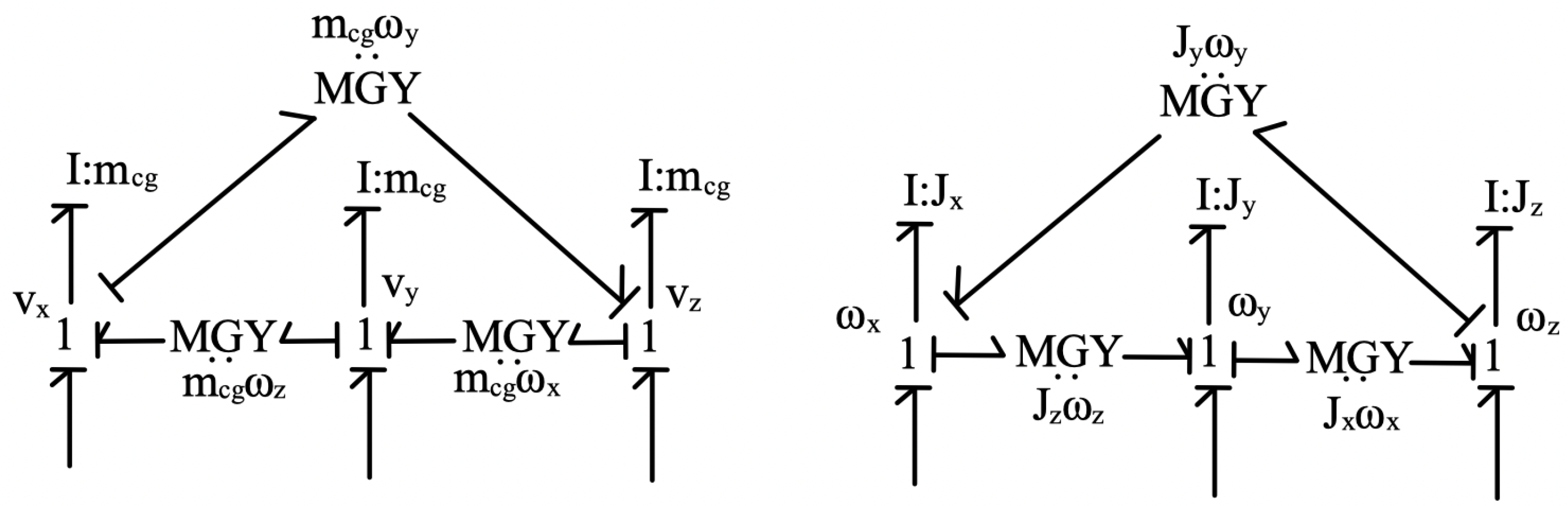
Figure 5 shows a back view of the hammer as it rotates towards the anvil. The velocity at the center of the hammer has been transferred from the center of gravity (CG) of the tool as indicated in Figure 2. The horizontal and vertical center velocity components, , , are then transferred to the hammer tine and then aligned in the tangent direction. The difference in the tangent direction velocity of the hammer and tangent direction velocity of the anvil is the relative velocity across the impact spring and damper. This construction is shown in the bond graph fragment of Figure 6.
In simulation, the hammer angle, , is tracked and when it is within 1of , impact is initiated. The impact advances the anvil depending on the retarding load specified on the anvil. Note that when testing the impact hammer, the anvil is often constrained to not move, i.e., the load on the anvil is infinite. This test condition is one of the simulations documented here.
The bond graph fragment in Figure 7 shows the motor/hammer interaction and uses a motor torque as the input to the motor inertia, . In the simulation, a simple controller keeps the motor angular velocity, , nearly constant unless motor control for vibration reduction was required. The motor angular velocity is reduced through the gearbox, , and the difference between the shaft angular rate, , and the hammer angular rate, , determines the vertical velocity of the hammer and is an input to the hammer spring. This is represented by the transformer, . At the bottom of Figure 7 is the anvil inertia and this is where the bond graph fragment from Figure 6 is attached.
Figure 7 also shows the interaction with the grip restraints indicated in Figure 2. Not shown in Figure 7 is the interaction with torsional constraints at the grip location and the restraints at the tip of the tool. The bond graph representation for these additional restraint elements is very similar to that for the grip constraints shown in Figure 7.
Causality has been assigned to the bond graph fragments of Figure 4, Figure 6, and Figure 7 and the state variables are dictated by the energy storage elements (I’s and C’s) in integral form. The state variables are identified here as:
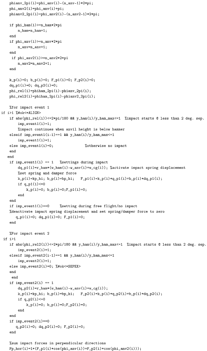
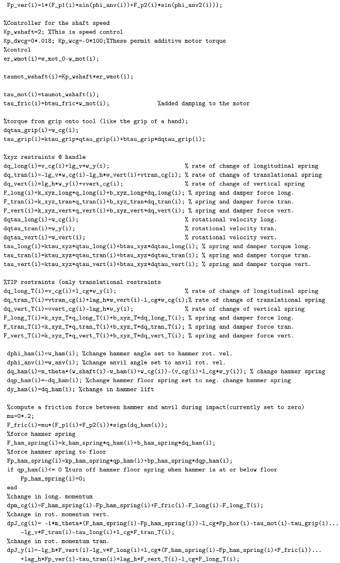
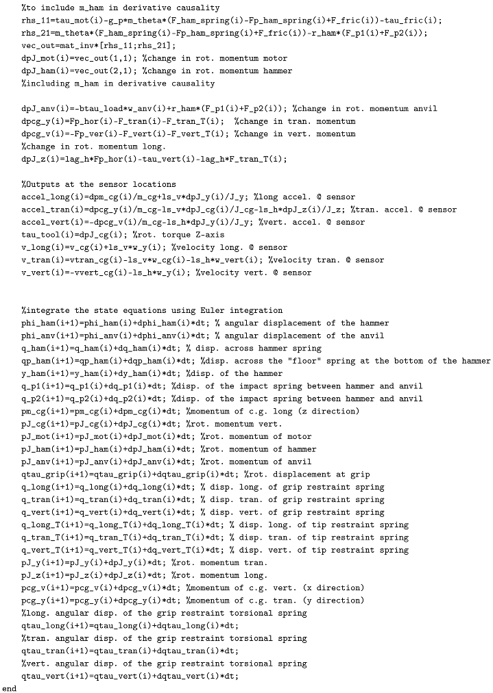
The first-order form of the state equations for these state variables is derived directly from the bond graph, Figure 8. Collecting the states into a vector and inputs (e.g., motor torque) into , the model can be expressed in the standard first-order form where denotes the parameter set in Table 1. Sample code of the model is given in Appendix A.
3. Impact Dynamics
The key dynamics of the impact hammer come from the impact between the hammer and anvil and the impact between the hammer and the ’floor’ of the hammer. Both of these impacts are modeled using very stiff impact springs with stiffness chosen through numerical simulation. For the impact between the hammer and anvil the state variables, and , are monitored and when is less than 1the impact spring is engaged and remains engaged until is greater than 1. The displacement of the hammer, , is also monitored and if becomes greater than the height of the anvil, the impact event is terminated. It is possible for the impact spring to be struck multiple times for a single impact event. It is also possible, following an impact event, for the hammer not to be below the anvil height after rotating 180and thus an impact event is missed. This logic is carried out for the 2 possible impact events per 360rotation of the hammer.
By monitoring the displacement of the hammer, , the impact with the floor spring can be determined. If the hammer displacement becomes less than 0 (hammer below the floor level), the floor impact spring is engaged and remains engaged until the hammer is no longer below the floor level. The floor impact spring stiffness was determined through numerical experimentation and declared stiff enough when penetration of the floor was less than a fraction of a millimeter.
Note that some damping was also part of the impact events and was chosen to reduce the ’ringing’ that accompanies inertias interacting with stiff springs.
4. Results
The first-order state equations were simulated using MATLAB. Parameters were representative of an impact hammer such as a Milwaukee M18FHIWF12-502X or Hilti SIW 6AT-A22. A simple motor controller was implemented to maintain a prescribed rotational speed of 13,500 RPM. The parameters for the grip constraints were tuned as best as possible to be representative of the hand/arm stiffness and damping. The tuned parameters were in the range of common values found in the literature [12].
In the first simulation a load was prescribed that allowed the anvil to rotate and come to rest with each impact event. Figure 9 shows the rotational angle of the hammer and the rotation of the anvil for the 2 impact events per full rotation of the hammer. This matches the expected interaction of the hammer and anvil teeth. The anvil teeth move in unison and they advance with the slope of the hammer movement.
Figure 10 shows the longitudinal motion of the hammer that results from the impact events. At t = 0, the hammer strikes the anvil floor at height zero. Then the hammer rebounds just over 1 mm. This process repeats continuously at approximately 32 Hz. The tool was observed to run at 42Hz under zero load. After testing under load the tool was observed to run at 32Hz.
Figure 11 shows the impact forces in the hammer return spring and in the impact spring at the hammer floor. In this simulation, the impact with the floor produces much larger forces than the force due to raising and lowering of the hammer spring. For this simulation, the vibration felt by the operator is primarily due to the hammer ’bottoming’ rather than the compression of the hammer spring.
Figure 12 shows the impact spring displacement between the hammer and anvil. The displacement is a fraction of a millimeter. For the negative displacement the impact spring stiffness and damping are set to zero as can be seen in Figure 13 for the force in the impact spring.
In the next simulation, the anvil is held fixed and does not advance upon impact. This is considered to be the test configuration and is used here for model verification. Figure 14 shows the z-direction, longitudinal motion of the hammer. In this simulation the hammer overshoots the anvil considerably and shows cycle to cycle variation.
Figure 15 shows the impact force between hammer and anvil for this test configuration. Comparing Figure 15 to Figure 13, the impact forces are much larger for the test configuration and much more erratic.
Figure 16, Figure 17 and Figure 18 show the frequency decomposition of the acceleration predicted at the sensor location in the three orthogonal directions. The acceleration signal was low-pass filtered prior to computing the frequency distribution. This is typical of the signal processing done when testing impact tools.
Test data were available for an impact hammer. The comparisons to predictions are shown next.
5. Model Verification
5.1. Test Setup:
The testing setup, Figure 19, is for the worst-case (highest vibration) scenario, similar to [17]. A new M20×40/8.8 bolt was threaded into a steel plate 20 mm thick. The bolt was bottomed out so as to no longer rotate while tightening. The impact wrench was held with the z-axis in the vertical direction. A 5000 g three-axis accelerometer was used to sample the signal. The sensor was mounted at the point on the handle where the thumb and index finger meet as per test standards. The signals were processed through a 30 kHz filter before recording. A sampling rate of s was used. Tests were performed for 8–10 s. A steady signal of 5 s was extracted for characterizing the user test.
5.2. Model Tuning:
The model has inputs for motor speed under load and two attachments (tip and handle) to the outside world that are tuned to match the test sample. The motor speed is tuned by matching the first mode of the frequency spectrum (42 Hz). The tip is tuned to be rigid in the x-, y-, and z-axis translational directions and free in rotation. The user hand forces (handle) are modeled by x-, y-, and z-axis translational and torsional spring-damper systems as shown in Figure 1. The frequencies of the systems are tuned to match each of the five different user grip forces. The model was run for a sweep using the frequency parameters (): x-axis: 1, 9, 17, 25 Hz; y-axis: 30, 34, 38, 42 Hz; z-axis: 60, 84, 108, 132 Hz. The spring constant, k, the damping constant, b, torsional spring constant, , and torsional damping constant, , are defined as:
The RMS accelerations in their respective directions (x, y, and z) for 5 s are compared to the test sample (Table 2). The closest RMS match for frequency values (Table 3) in each respective axis was used (Table 4). Closer matches could be found if a finer sweep were performed. The matches found were within the standard allowable tolerance of ±15% error in the RMS for each respective axis (Table 5).
5.3. Spectral Amplitude Frequency Distribution
The spectral amplitude frequency distributions in their respective directions (x, y, and z) for 5 s are compared between the five test samples and the tuned model (Figure 20, Figure 21, Figure 22, Figure 23 and Figure 24). The frequency modes up to 200 Hz are compared. The first 4.5 modes are present in the frequency distribution between 0 Hz and 200 Hz. The test signal contains noise due to the signal amplification. The comparison shows that each mode (approximately 42 Hz) and each half mode are accurately represented by the model. The relative magnitudes of each mode deviate between the test samples and the model. This likely stems from the difference in damping between the real system and the estimates necessary when modeling a system. Further tuning of the damping parameters of the model could alleviate this discrepancy. This is not a necessary step to compare different vibration reduction strategies.
6. Discussion
The validated, low-order model captures both RMS accelerations and modal content up to 200 Hz with errors within 11%, which is sufficient for comparative design evaluation. The results indicate that: (i) the translational (z-axis) impact is a dominant contributor to perceived vibration while not essential for tightening; (ii) rotational impacts can be mitigated via damping or control without compromising function [18]; and (iii) realistic hand/arm coupling is crucial to reproduce axis-wise spectra [19,20]. Practically, the model predicts axis-wise RMS values and spectral peaks prior to hardware builds, supporting pre-compliance iteration against ISO 28927-13 and aligning with historical ISO 8662-7 procedure development [21]. Design changes suggested by the model include removing the linear impact path, increasing rotational damping, and tuning hand/handle impedance through geometry or compliant interfaces.
7. Conclusions
The tuned model RMS acceleration over 5 s matches the validation data in the x-, y-, and z-axes with near-perfect agreement (<11%) in each of the five test cases. A perfect match would be attainable if the hand input parameters were further tuned and more sophisticated modeling of the hand/arm were performed. A perfect match is not necessary since the user hand force variability is much larger (>15%) than the deviation of the model from the test data. It would be advisable to use several variations of the hand input tuning parameters to capture an accurate representation of real-world HAV.
This model shows that the major component of the HAV originates from the impact of the hammer on the anvil in the z-axis. This is notable because the force required to tighten the bolt occurs only in the x- and y-axes. It is conceivable that a vibration mitigation solution that reduces or eliminates the z-axis vibrations would not affect the hammering performance. This model can now be confidently used to analyze the effectiveness of vibration reduction concepts. Future work could capture the wave of frequencies that are visible in the test data below 20 Hz. This would mainly come from tuning the damping in the model.
Industrial Relevance.
The proposed low-order model provides a fast, insight-oriented tool to iterate power-tool mechanisms and handle interfaces before building hardware. The model predicts axis-wise RMS accelerations and spectral peaks aligned with ISO 28927-13, enabling designers to down-select mitigation strategies (e.g., eliminating the linear impact, adding rotational damping/control, tuning handle impedance) with quantitative expectations for reduction in HAV exposure and improved user comfort.
8. Acknowledgements
This research did not receive any specific grant from funding agencies in the public, commercial, or not-for-profit sectors.
Author Contributions
Conceptualization, T.T.B. and D.L.M.; methodology, D.L.M.; formal analysis, T.T.B.; data curation, T.T.B.; writing—original draft preparation (introduction, model verification, conclusions), T.T.B.; writing—model development, simulation and impact dynamics, D.L.M.; supervision, D.L.M.; project administration, T.T.B. All authors have read and agreed to the published version of the manuscript.
Funding
This research received no external funding.
Data Availability Statement
Data contain proprietary tool information and are available from the corresponding author upon reasonable request, subject to owner approval.
Conflicts of Interest
The authors declare no conflict of interest.
Abbreviations
The following abbreviations are used in this manuscript:
| HAV | Hand-Arm Vibrations |
| I | Inertance |
| C | Capacitance |
| R | Resistance |
| RMS | Root Mean Square |
| g | gravity |
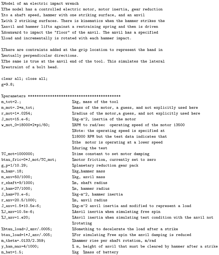
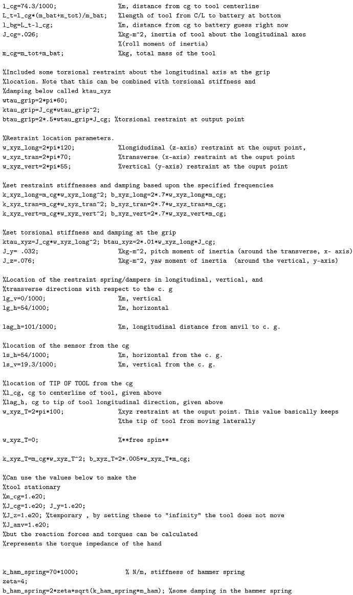
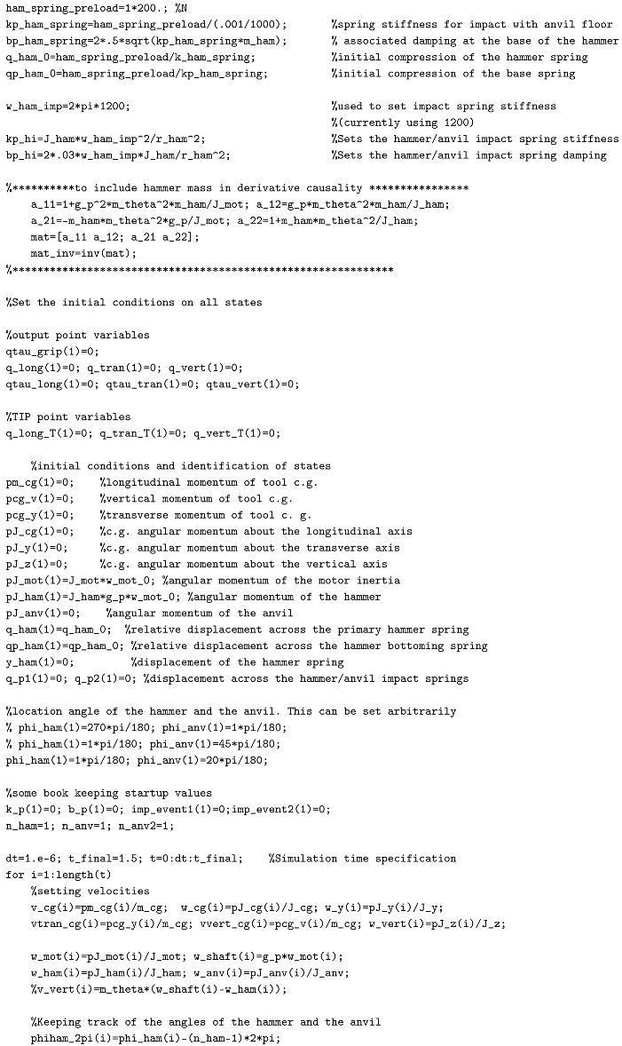
Appendix A Example Code of Model
References
- Matthiesen, S.; Wettstein, A.; Grauberger, P. Analysis of dynamic system behaviour using sequence modelling with the C&C2-Approach - a case study on a power tool hammer mechanism. In Proceedings of the Proceedings of NordDesign: Design in the Era of Digitalization, NordDesign 2018; The Design Society, 2018. [Google Scholar]
- Weir, E.; Lander, L. Hand–arm vibration syndrome. CMAJ 2005, 172, 1001–1002. [Google Scholar] [CrossRef] [PubMed]
- Vihlborg, P.; Bryngelsson, I.L.; Lindgren, B.; Gunnarsson, L.G.; Graff, P. Association between vibration exposure and hand-arm vibration symptoms in a Swedish mechanical industry. International Journal of Industrial Ergonomics;Prevention and Intervention of Hand-Arm Vibration Injuries and Disorders 2017, 62, 77–81. [Google Scholar] [CrossRef]
- Nilsson, T.; m, J.; m, L. Hand-arm vibration and the risk of vascular and neurological diseases-A systematic review and meta-analysis. PLoS One 2017, 12, e0180795. [Google Scholar] [CrossRef] [PubMed]
- Krajnak, K.M.; Waugh, S.; Johnson, C.; Miller, G.R.; Xu, X.; Warren, C.; Dong, R.G. The effects of impact vibration on peripheral blood vessels and nerves. Ind Health 2013, 51, 572–580. [Google Scholar] [CrossRef] [PubMed]
- Vergara, M.; Sancho, J.L.; Rodríguez, P.; Pérez-González, A. Hand-transmitted vibration in power tools: Accomplishment of standards and users’ perception. International Journal of Industrial Ergonomics;Special Issue: Workplace Vibration Exposure Characterization, assessment and ergonomic interventions 2008, 38, 652–660. [Google Scholar] [CrossRef]
- Mazaheri, A.; Rose, L. Reaction load exposure from handheld powered tightening tools: A scoping review. International Journal of Industrial Ergonomics 2021, 81, 103061. [Google Scholar] [CrossRef]
- Rimell, A.N.; Notini, L.; Mansfield, N.J.; Edwards, D.J. Variation between manufacturers’ declared vibration emission values and those measured under simulated workplace conditions for a range of hand-held power tools typically found in the construction industry. International Journal of Industrial Ergonomics;Special Issue: Workplace Vibration Exposure Characterization, assessment and ergonomic interventions 2008, 38, 661–675. [Google Scholar] [CrossRef]
- Clemm, T.; Færden, K.; Ulvestad, B.; Lunde, L.; Nordby, K. Dose–response Relationship between Hand–Arm Vibration Exposure and Vibrotactile Thresholds among Roadworkers. Occupational and Environmental Medicine 2020, 77, 188–193. [Google Scholar] [CrossRef] [PubMed]
- Clemm, T.; Lunde, L.; Ulvestad, B.; Færden, K.; Nordby, K. Exposure–Response Relationship between Hand–Arm Vibration Exposure and Vibrotactile Thresholds among Rock Drill Operators: A 4-Year Cohort Study. Occupational and Environmental Medicine 2022, 79, 775–781. [Google Scholar] [CrossRef]
- Faik, S.; Witteman, H.O. Modeling of Impact Dynamics: A Literature Survey; 2000. [Google Scholar]
- Rakheja, S.; WU, J.; Dong, R.; SCHOPPER, A.; Boileau, P.E. Comparison of biodynamic models of the human hand-arm system for applications to hand-held power tools. Journal of Sound and Vibration 2002, 249, 55–82. [Google Scholar] [CrossRef]
- Zhang, S.; Tang, J. System-Level Modeling and Parametric Identification of Electric Impact Wrench. Journal of Manufacturing Science and Engineering 2016, 138, 111010. [Google Scholar] [CrossRef]
- Karnopp, D.C.; Margolis, D.L.; Rosenberg, R.C. System Models. In System Dynamics; John Wiley and Sons, Ltd, 2012; Volume chapter 4, pp. 77–161. [Google Scholar] [CrossRef]
- Zhang, S.; Tang, J. Dynamic Modeling of Torsional Impact and Its Stiffness Measurement for Impact Wrench. In Proceedings of the Proceedings of the ASME 2015 Dynamic Systems and Control Conference (DSCC2015), Columbus, OH, USA, October 2015; pp. Paper No. DSCC2015–10000. [Google Scholar]
- Wallace, P. Energy, Torque, and Dynamics in Impact Wrench Tightening. Journal of Manufacturing Science and Engineering 2015, 137, 024503. [Google Scholar] [CrossRef]
- McDowell, T.W.; Dong, R.G.; Xu, X.; Welcome, D.E.; Warren, C. An Evaluation of Impact Wrench Vibration Emissions and Test Methods. The Annals of Occupational Hygiene 2008, 52, 125–138. [Google Scholar] [CrossRef] [PubMed]
- Moschioni, G.; Saggin, B.; Tarabini, M.; Marrone, M. Reduction of Vibrations Generated by an Impact Wrench. Canadian Acoustics / Acoustique canadienne 2011, 39, 82–83. [Google Scholar]
- Adewusi, S.; Rakheja, S.; Marcotte, P.; Thomas, M. Distributed Vibration Power Absorption of the Human Hand-Arm System in Different Postures Coupled with Vibrating Handle and Power Tools. International Journal of Industrial Ergonomics 2013, 43, 363–374. [Google Scholar] [CrossRef]
- Raffler, N.; Wilzopolski, T.; Freitag, C. Using an Impact Wrench in Different Postures—An Analysis of Awkward Hand–Arm Posture and Vibration. Proceedings 2023, 86, 40. [Google Scholar] [CrossRef]
- McDowell, T.W.; Dong, R.G.; Xu, X.; Welcome, D.E.; Warren, C. Evaluating Impact Wrench Vibration Using the Method in Proposed Revisions to ISO 8662-7. In Proceedings of the Conference paper, National Institute for Occupational Safety and Health (NIOSH), Morgantown, WV, USA, June 2008. [Google Scholar]
Figure 1.
Flow diagram of procedure.
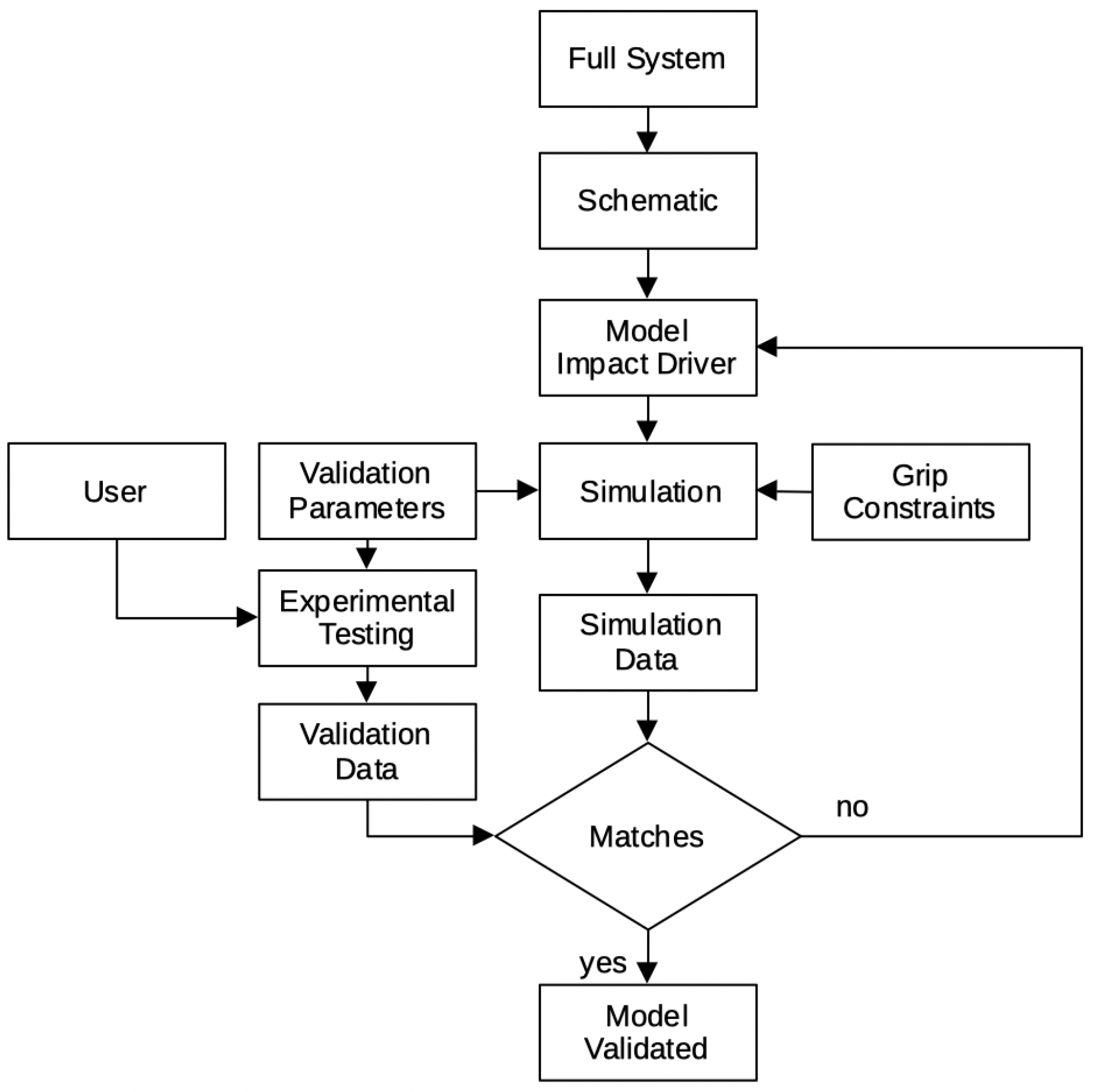
Figure 2.
Schematic of impact hammer with coordinates and lengths identified.
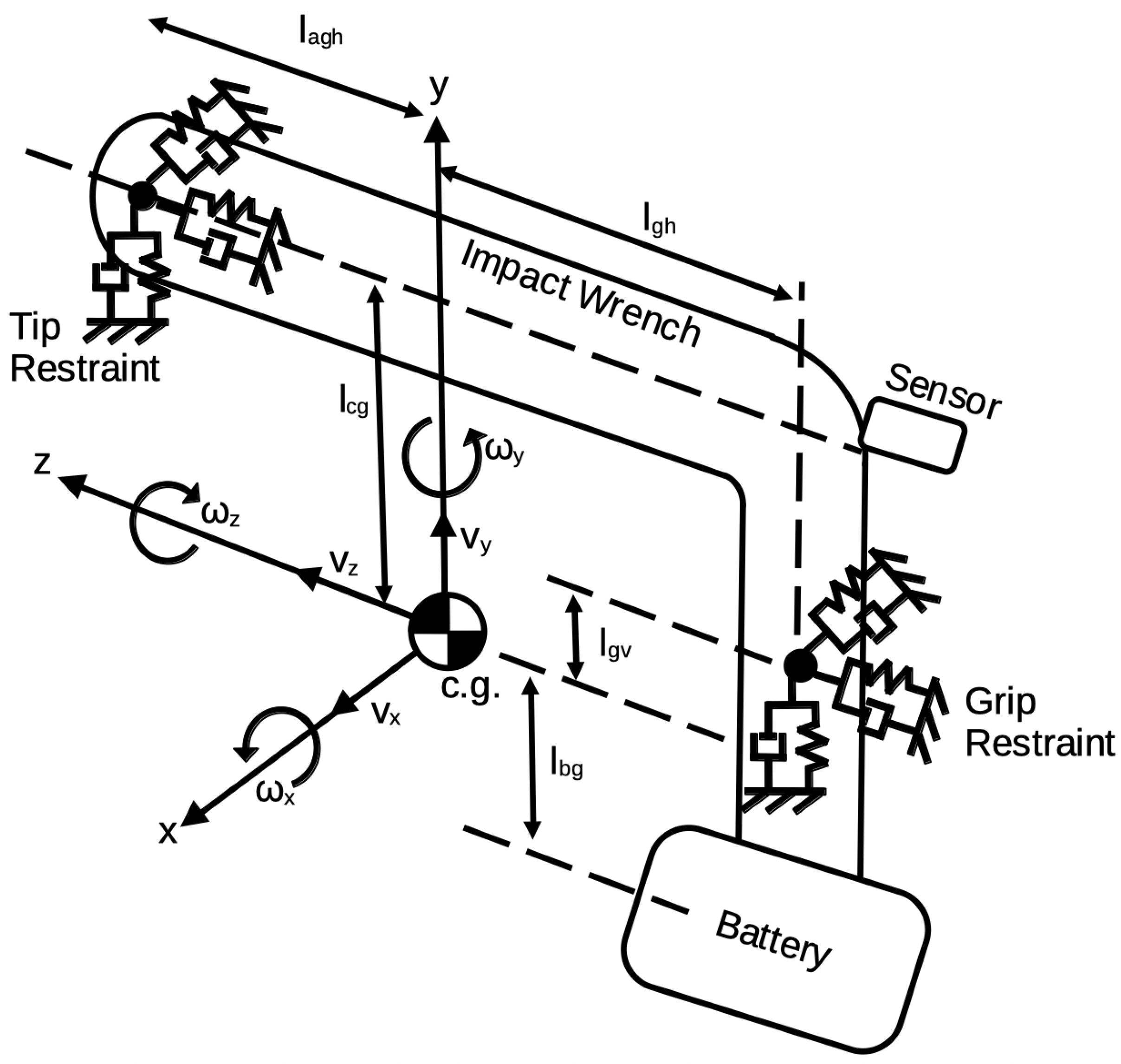
Figure 3.
Schematic showing the internal dynamic elements of the impact hammer.
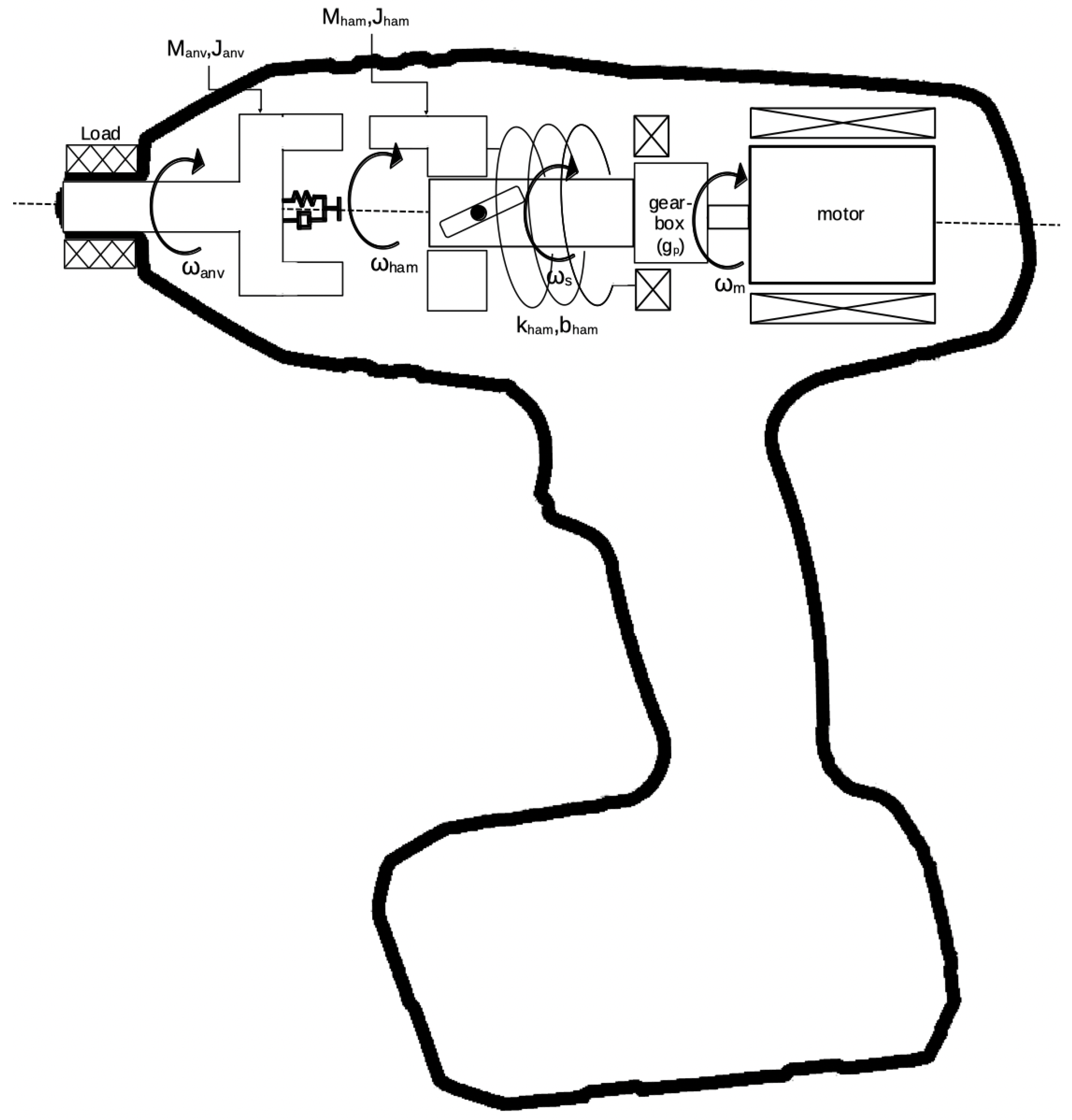
Figure 5.
Back view of the hammer as it approaches the anvil for impact.
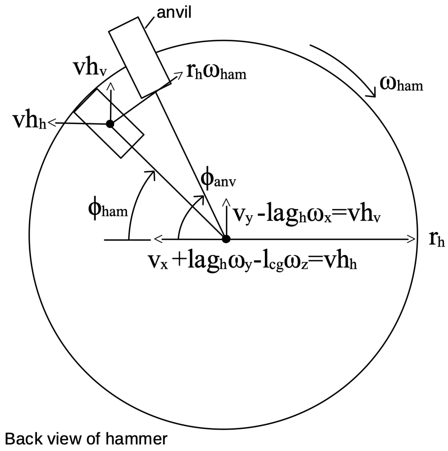
Figure 6.
Bond graph fragment coupling the rigid body kinematics with the hammer/anvil interaction.
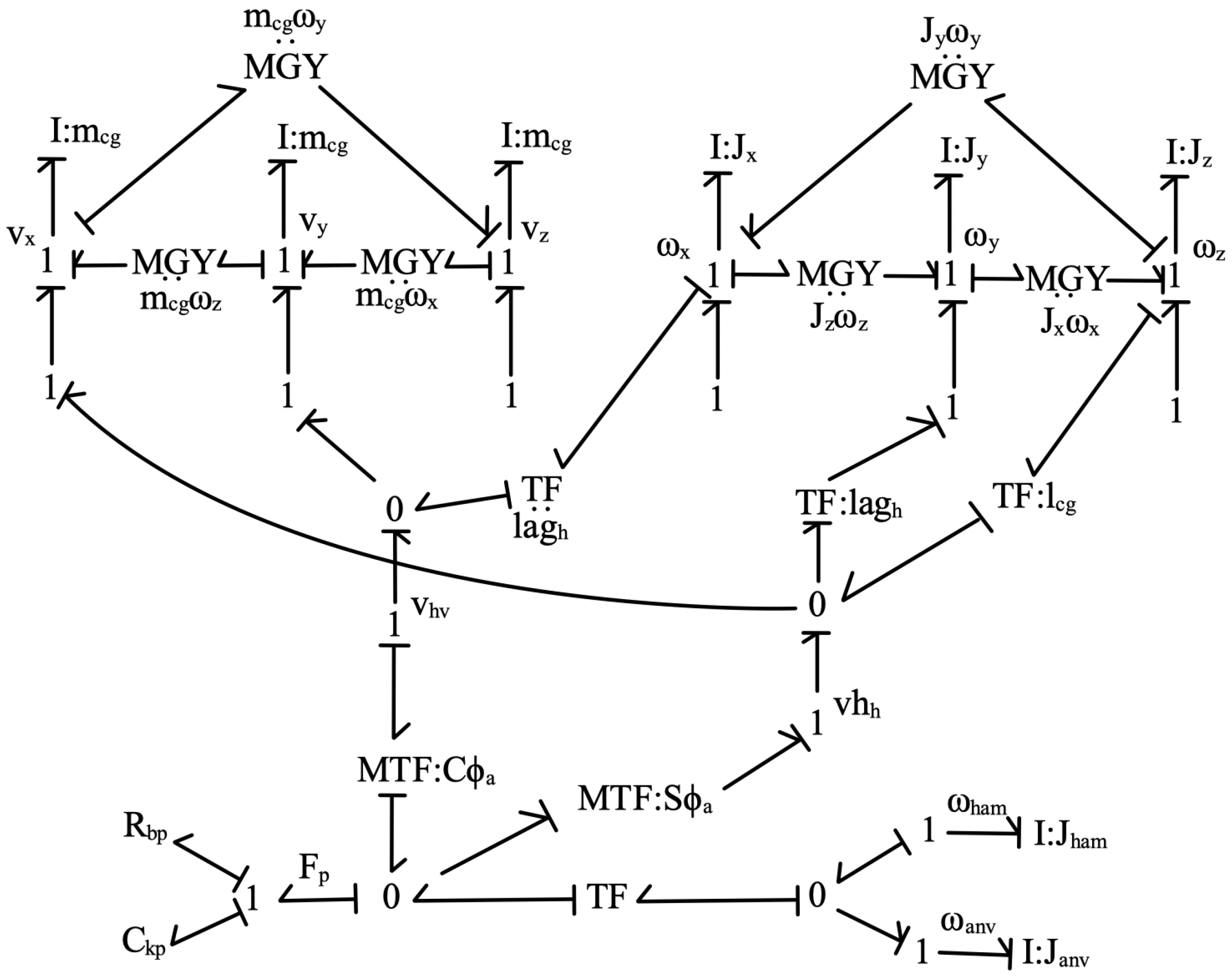
Figure 7.
Bond graph fragment showing the dynamics of the hammer spring and the interaction with the hand/arm constraints.
Figure 7.
Bond graph fragment showing the dynamics of the hammer spring and the interaction with the hand/arm constraints.
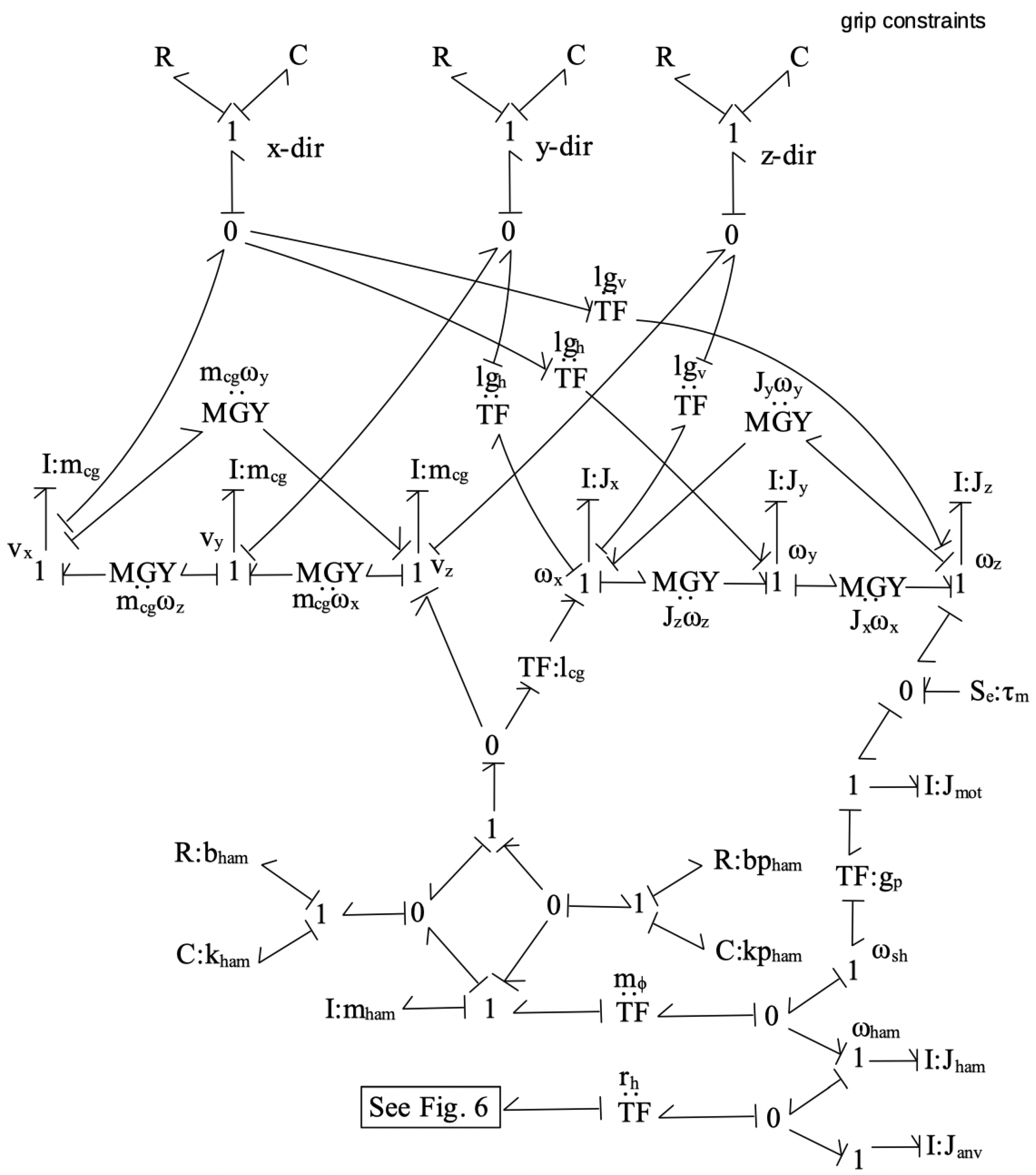
Figure 8.
First order states.
Figure 9.
Angular rotation of the hammer and anvil due to repeated impact events.
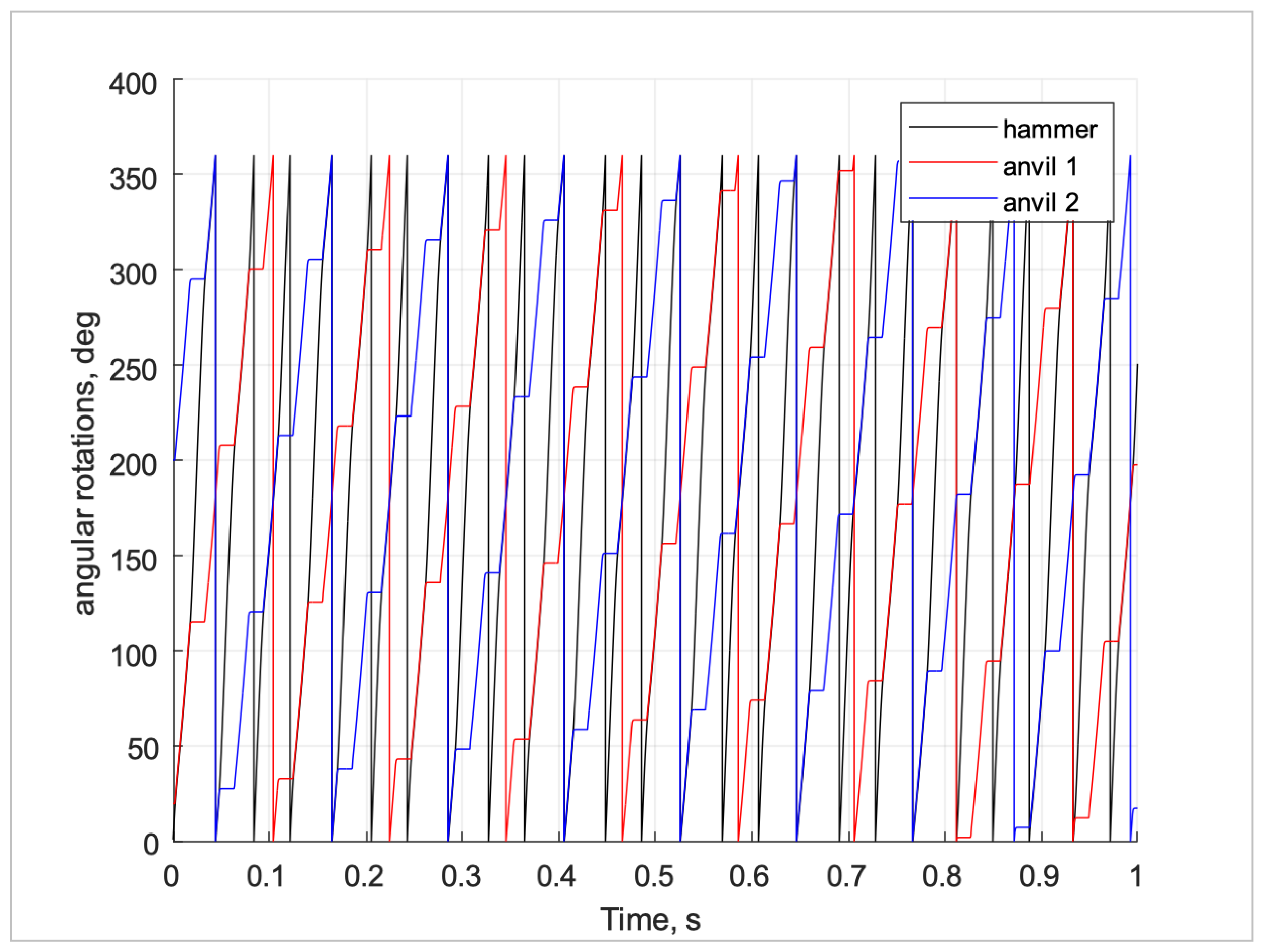
Figure 10.
z-direction, longitudinal hammer motion resulting from the impact events.
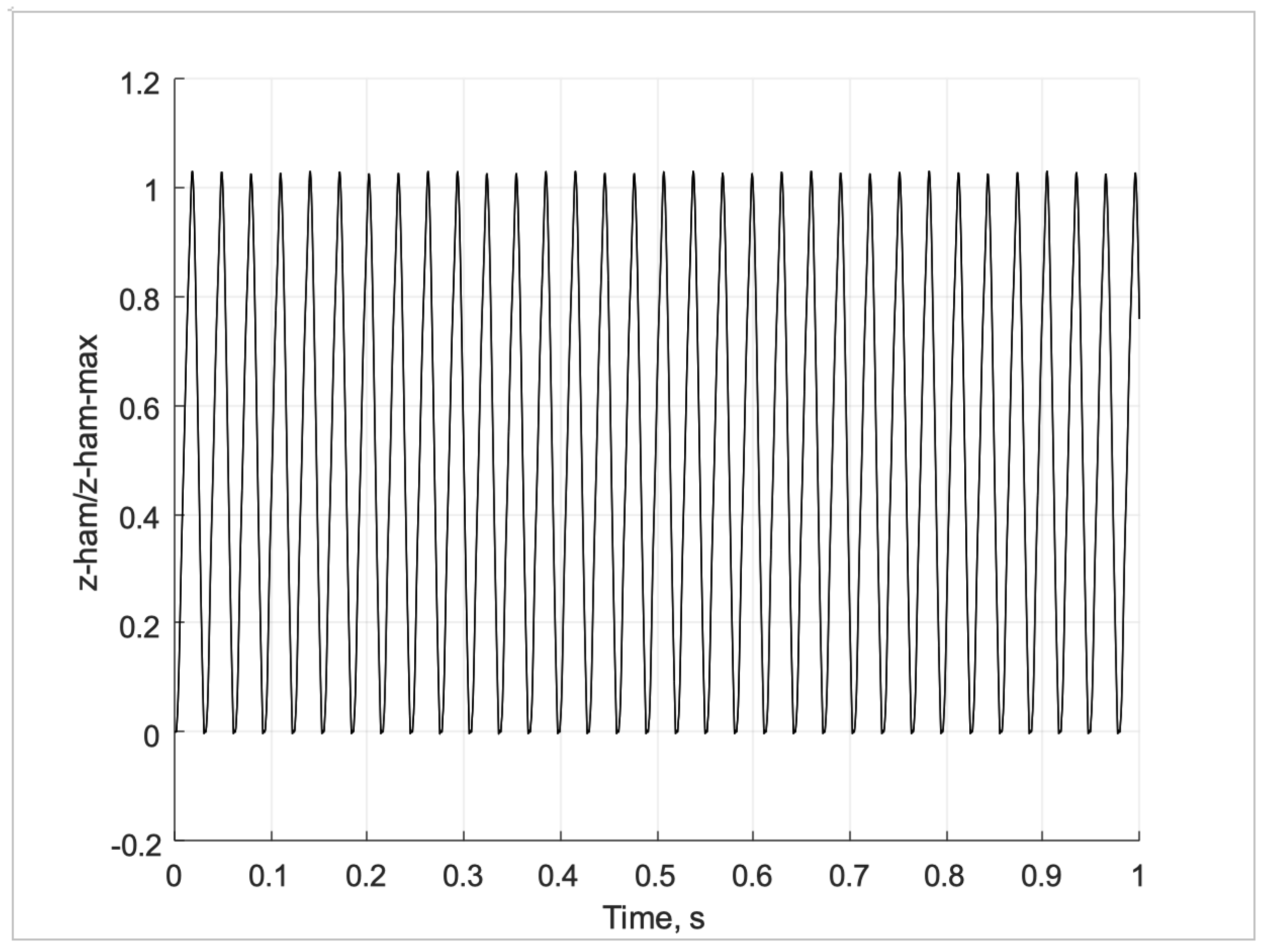
Figure 11.
Force in the hammer spring and the ”floor” impact spring.
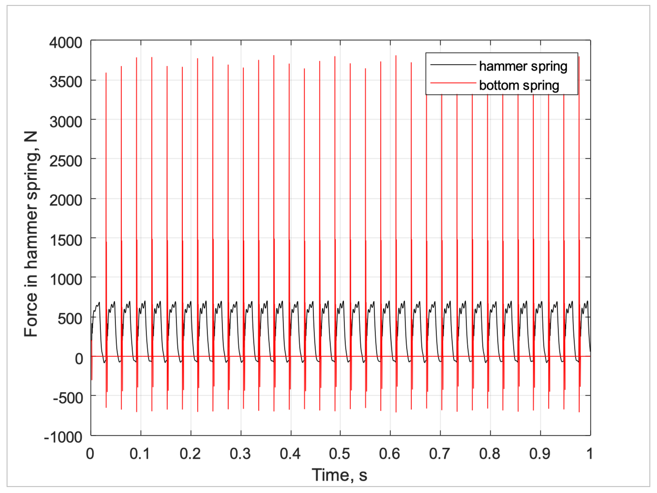
Figure 12.
Displacement of the impact spring between hammer and anvil.
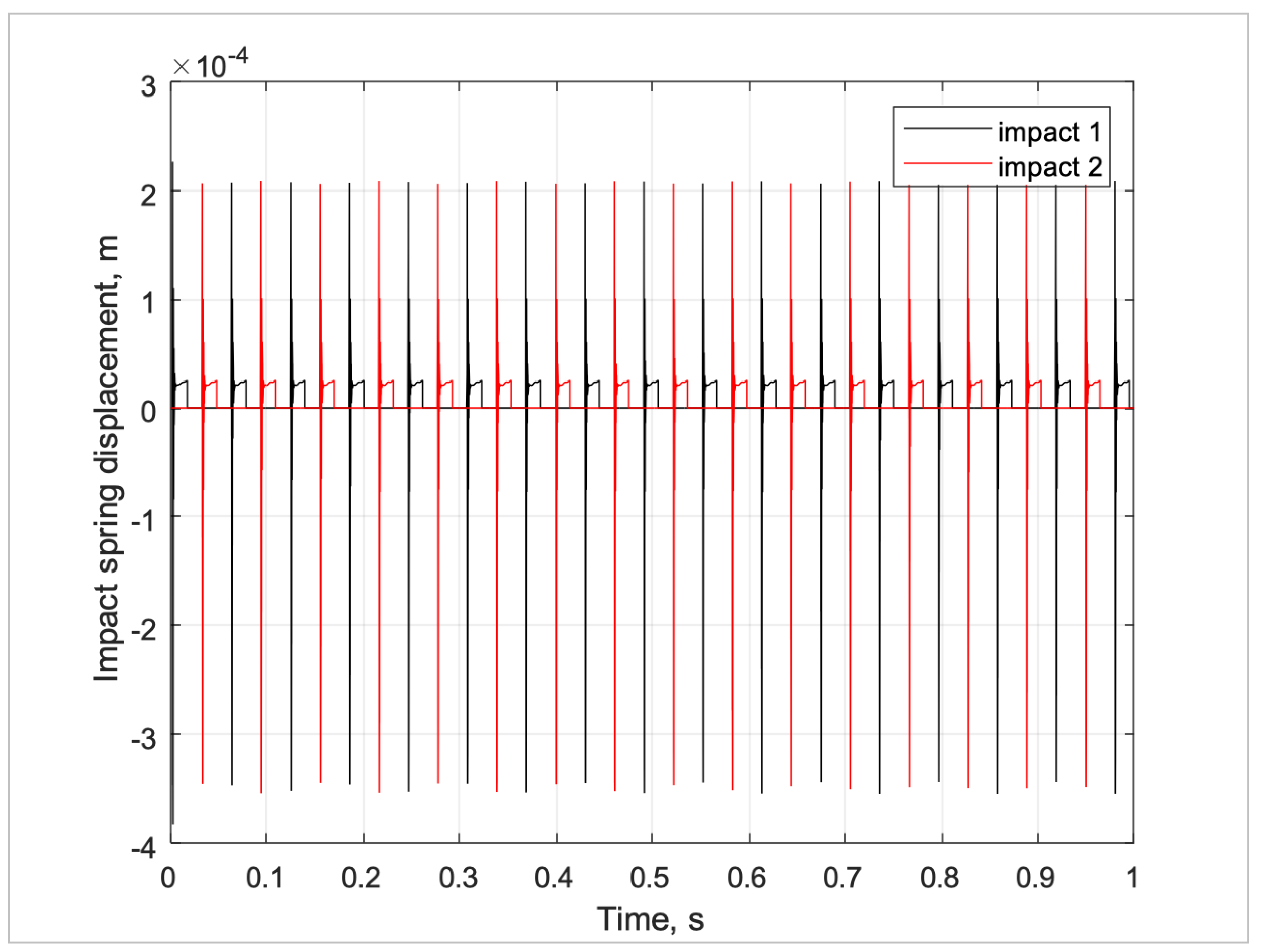
Figure 13.
Force in the impact spring/damper between hammer and anvil.

Figure 14.
z-direction, longitudinal hammer motion resulting from the impact events for test configuration.
Figure 14.
z-direction, longitudinal hammer motion resulting from the impact events for test configuration.

Figure 15.
Impact force between hammer and anvil for the test configuration with anvil stationary.
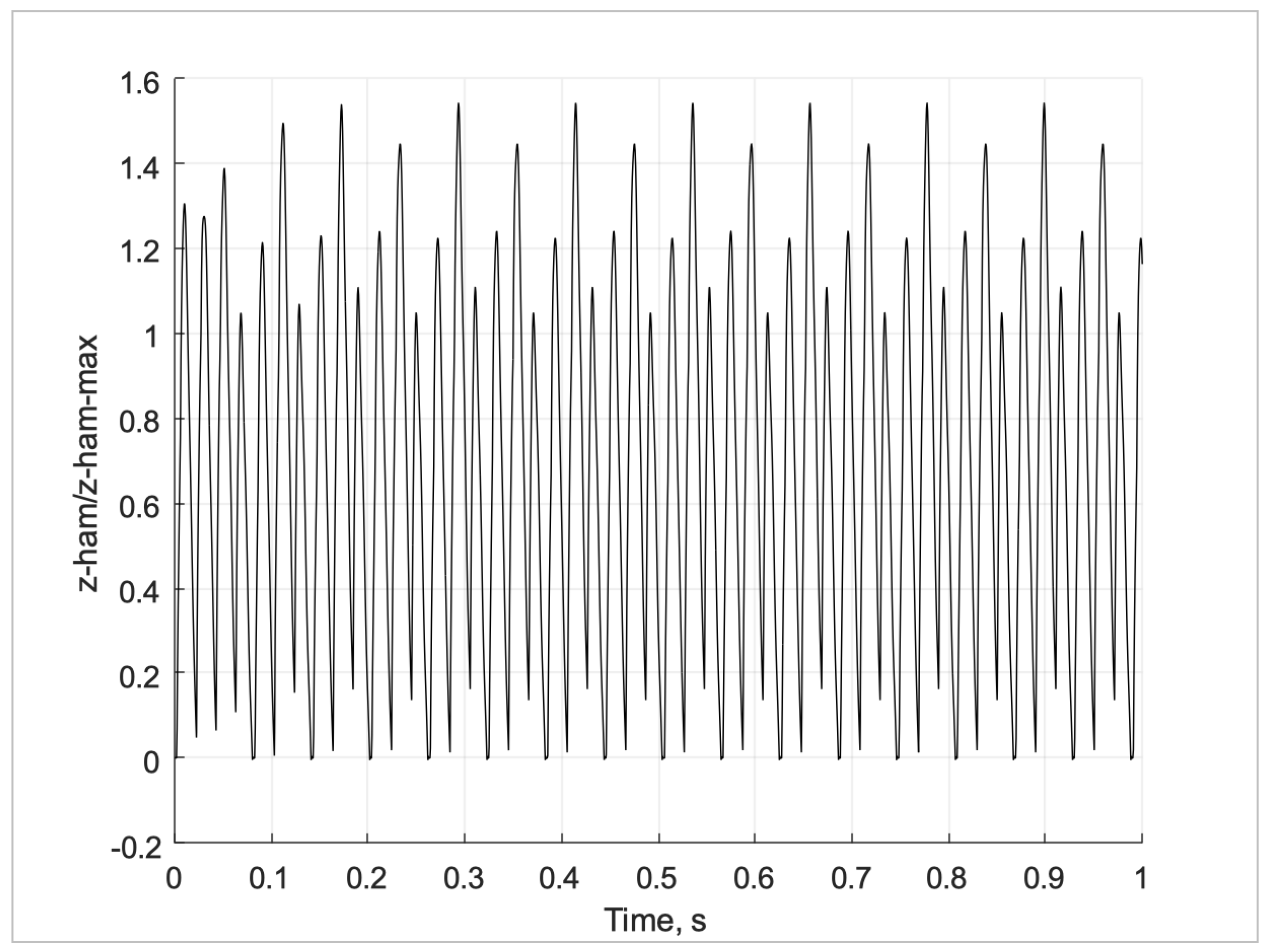
Figure 16.
Frequency distribution of the longitudinal z-direction acceleration at the sensor location.
Figure 16.
Frequency distribution of the longitudinal z-direction acceleration at the sensor location.
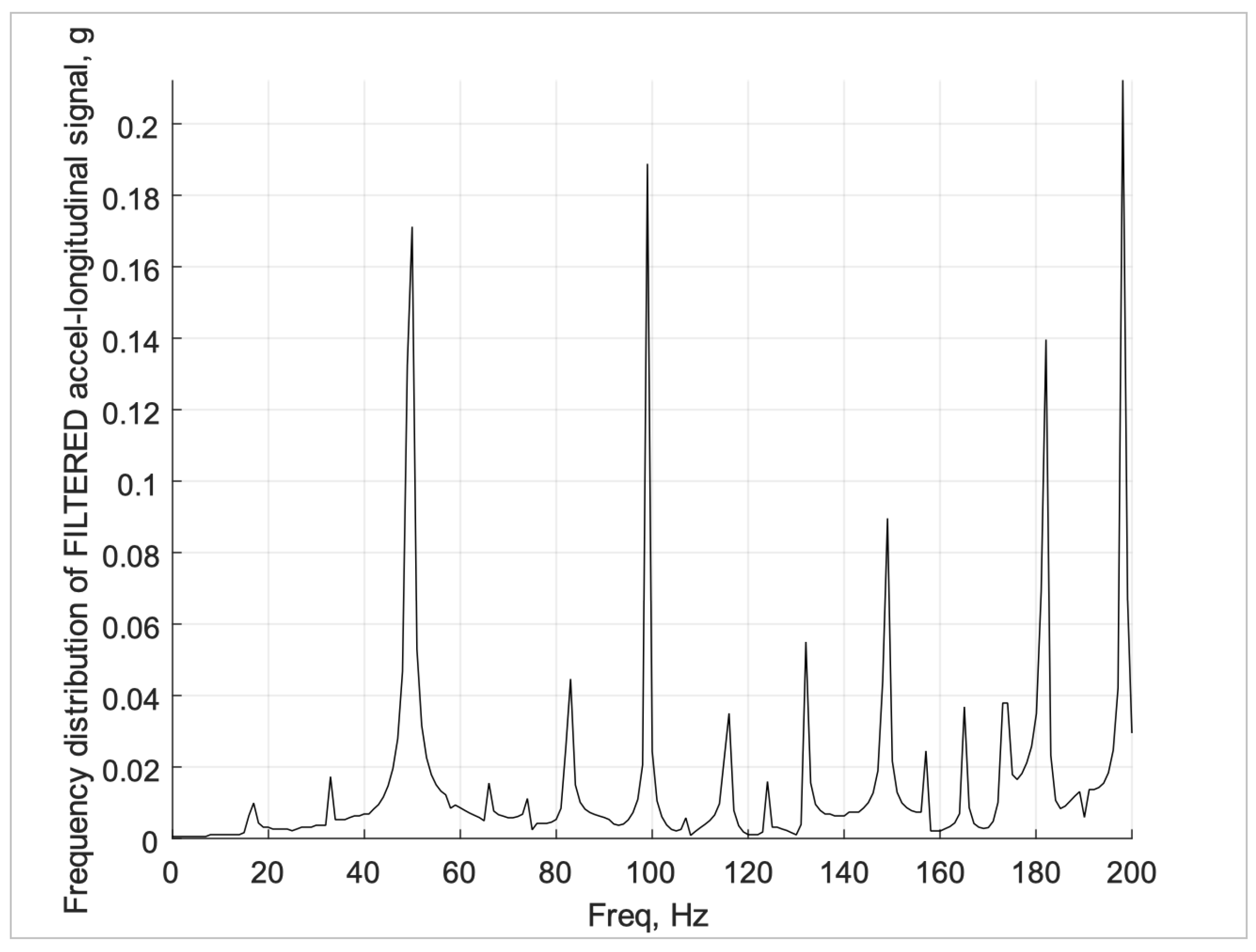
Figure 17.
Frequency distribution of the transverse x-direction acceleration at the sensor location.
Figure 17.
Frequency distribution of the transverse x-direction acceleration at the sensor location.
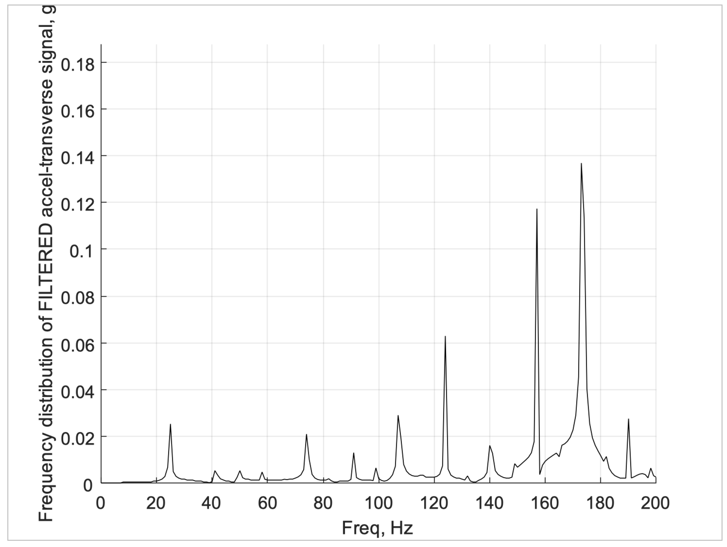
Figure 18.
Frequency distribution of the vertical y-direction acceleration at the sensor location.
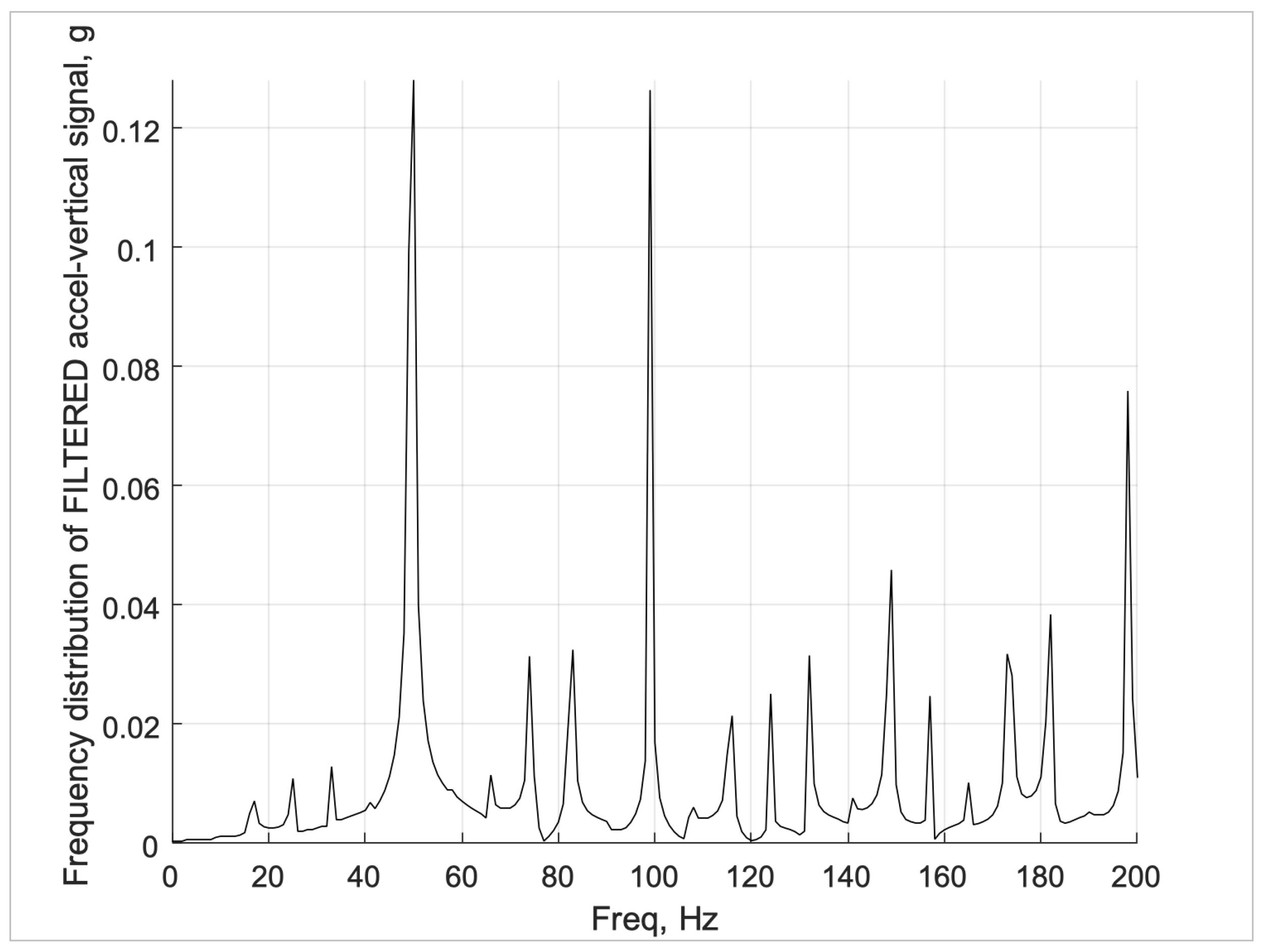
Figure 19.
Test setup layout.
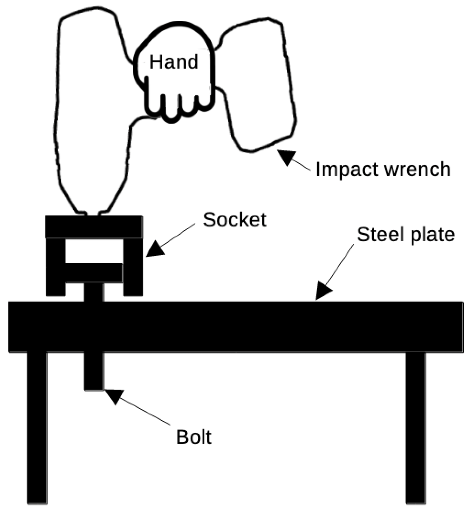
Figure 20.
User test vs model tuned to user sample 1.
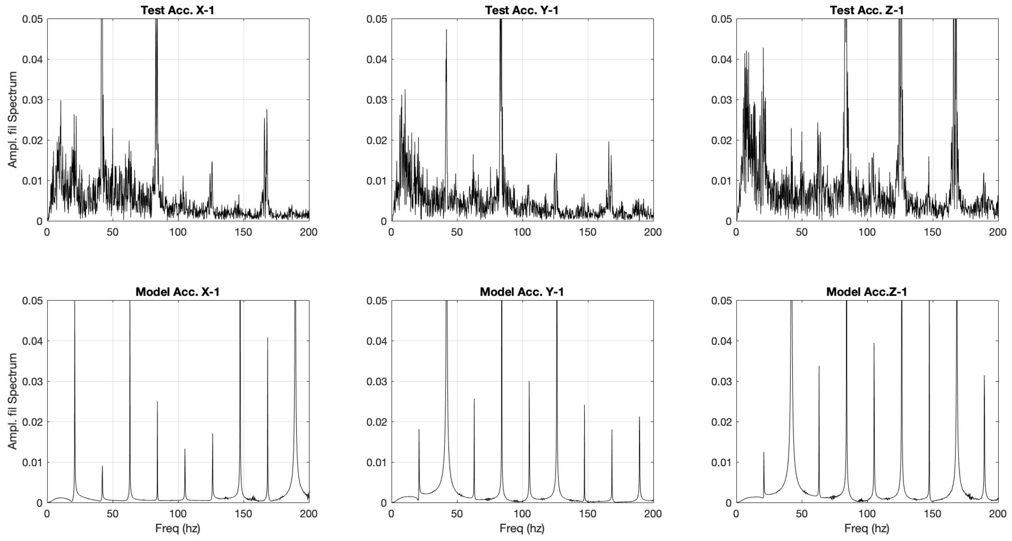
Figure 21.
User test vs model tuned to user sample 2.
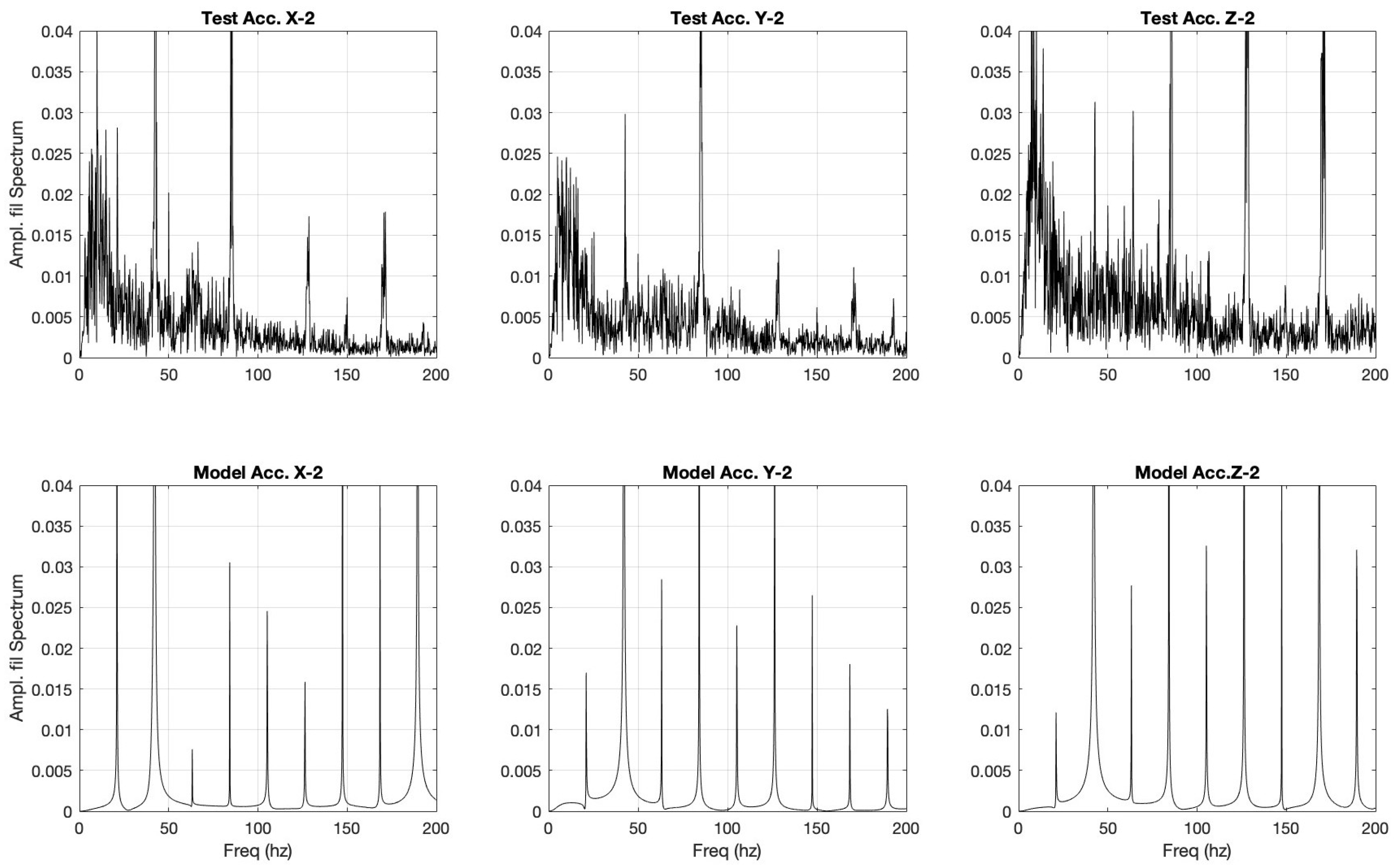
Figure 22.
User test vs model tuned to user sample 3.
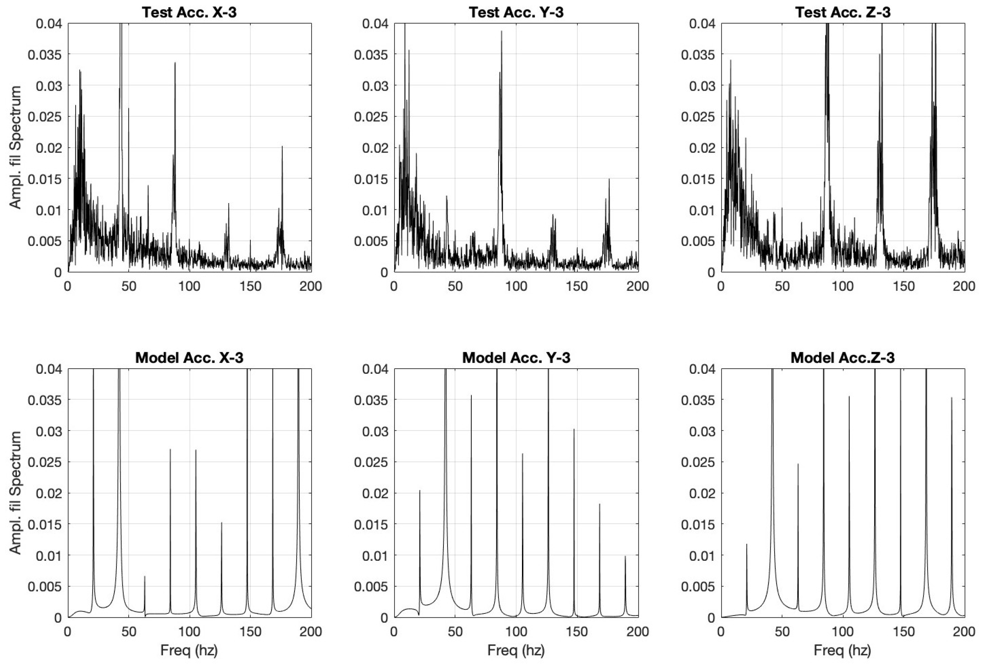
Figure 23.
User test vs model tuned to user sample 4.
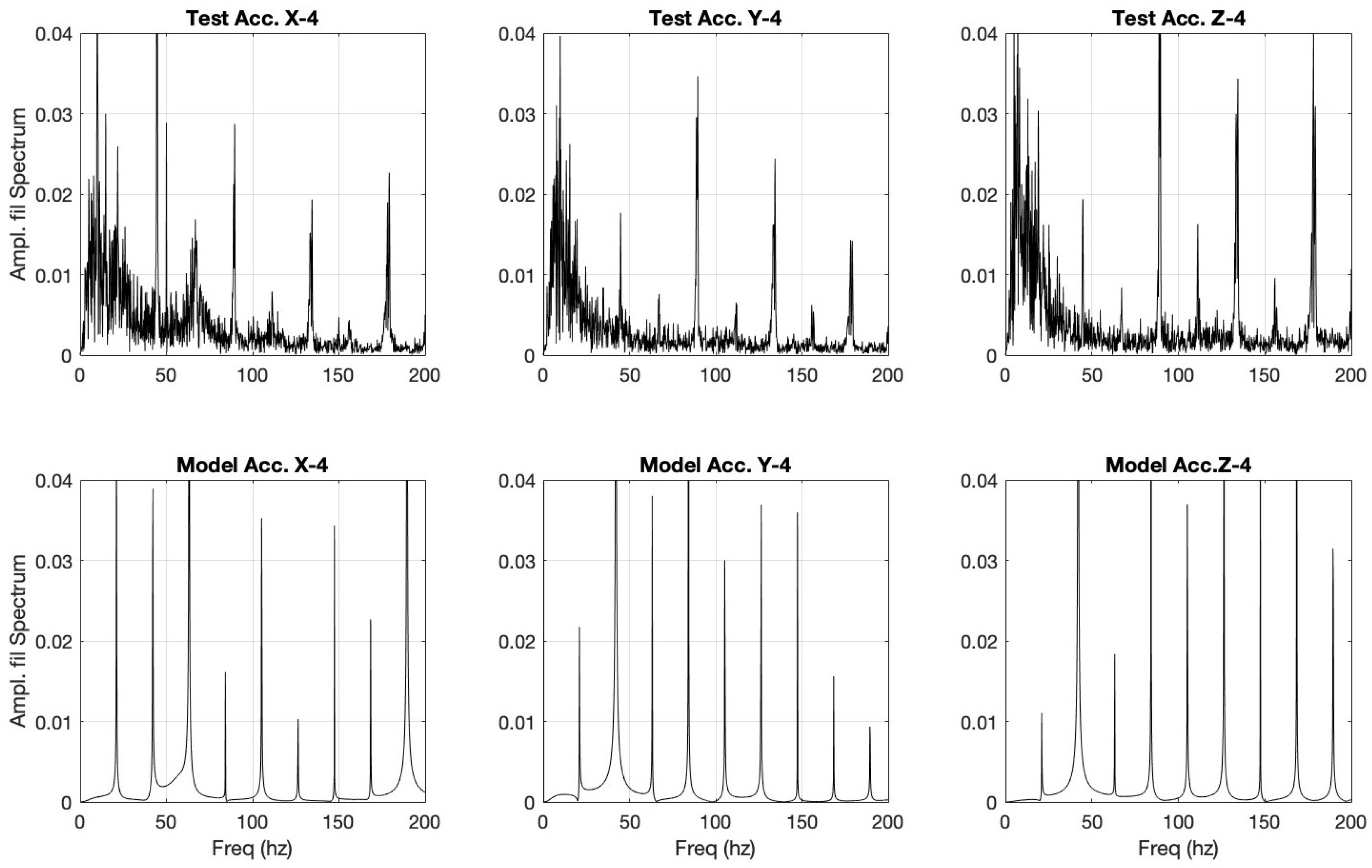
Figure 24.
User test vs model tuned to user sample 5.
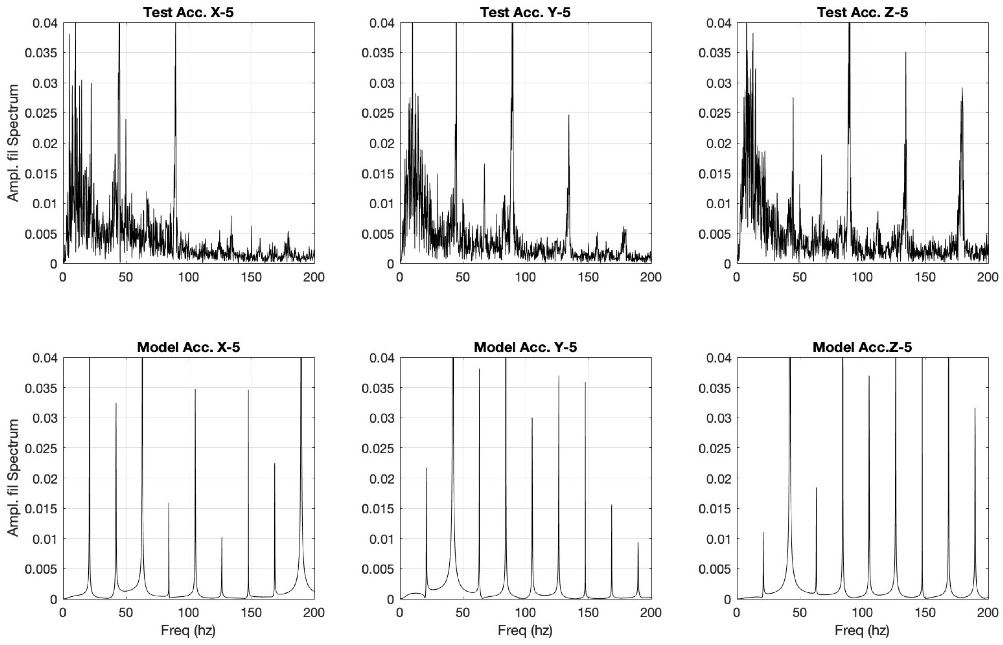

Table 1.
Key model parameters used in simulations.
| Quantity | Value |
|---|---|
| Motor nominal speed, | 13 500 RPM (validated) |
| Gear ratio, | 1/10.29 |
| Hammer mass, | 0.18 kg |
| Hammer spring stiffness, | 70 kN/m |
| Hammer spring damping ratio, | 4 |
| Impact stiffness (hammer/anvil), | set via rad/s |
| Anvil inertia, | kg m2 (load-modified) |
| Grip translational frequencies (x,y,z) | (70, 55, 120) Hz |
| Tip translational frequency | 0 Hz (free spin) |
Table 2.
RMS Accelerations User Tests (Fixed anvil during 5 second samples measured in g’s).
| Sample # | x-axis | y-axis | z-axis |
|---|---|---|---|
| 1 | 0.58 | 0.51 | 0.88 |
| 2 | 0.59 | 0.40 | 0.65 |
| 3 | 0.65 | 0.46 | 0.61 |
| 4 | 0.53 | 0.40 | 0.49 |
| 5 | 0.47 | 0.43 | 0.51 |
Table 3.
Model User Parameters (Hz): Frequency tuning values for each model for each test sample.
| Sample # | x-axis | y-axis | z-axis |
|---|---|---|---|
| 1 | 17 | 30 | 60 |
| 2 | 2 | 42 | 90 |
| 3 | 2 | 34 | 95 |
| 4 | 9 | 38 | 132 |
| 5 | 17 | 38 | 132 |
Table 4.
RMS Accelerations Model Simulations (Fixed anvil during 5 second samples measured in g’s).
| Sample # | x-axis | y-axis | z-axis |
|---|---|---|---|
| 1 | 0.57 | 0.51 | 0.93 |
| 2 | 0.59 | 0.41 | 0.72 |
| 3 | 0.62 | 0.48 | 0.68 |
| 4 | 0.52 | 0.40 | 0.52 |
| 5 | 0.47 | 0.40 | 0.52 |
Table 5.
Errors between User tests and model simulations (Fixed anvil during 5 seconds measured in g’s).
Table 5.
Errors between User tests and model simulations (Fixed anvil during 5 seconds measured in g’s).
| Sample # | x-axis | y-axis | z-axis |
|---|---|---|---|
| 1 | -0.02 | 0.00 | 0.06 |
| 2 | 0.00 | 0.02 | 0.11 |
| 3 | -0.05 | -0.02 | 0.00 |
| 4 | 0.04 | 0.00 | 0.06 |
| 5 | 0.00 | -0.07 | 0.02 |
Disclaimer/Publisher’s Note: The statements, opinions and data contained in all publications are solely those of the individual author(s) and contributor(s) and not of MDPI and/or the editor(s). MDPI and/or the editor(s) disclaim responsibility for any injury to people or property resulting from any ideas, methods, instructions or products referred to in the content. |
© 2026 by the authors. Licensee MDPI, Basel, Switzerland. This article is an open access article distributed under the terms and conditions of the Creative Commons Attribution (CC BY) license (http://creativecommons.org/licenses/by/4.0/).
Copyright: This open access article is published under a Creative Commons CC BY 4.0 license, which permit the free download, distribution, and reuse, provided that the author and preprint are cited in any reuse.


