
Submitted:
29 December 2025
Posted:
31 December 2025
You are already at the latest version
Abstract
In the theory of mixed-type equations, there are many works in bounded domains with smooth boundaries bounded by a normal curve for first and second-kind mixed-type equations. In this paper, for a second-kind mixed-type equation in an unbounded domain whose elliptic part is a horizontal half-strip, a Bitsadze-Samarskii type problem is investigated. The uniqueness of the solution is proved using the extremum principle, and the existence of the solution is proved by the Green’s function method and the integral equations method. When constructing the Green’s function, the properties of Bessel functions of the second kind with imaginary argument and the properties of the Gauss hypergeometric function are widely used. Visualization of the solution to the Bitsadze-Samarskii type problem is performed, confirming its correctness from both mathematical and physical points of view.
Keywords:
Bitsadze-Samarskii problem
; second-kind mixed-type equation
; extremum principle
; Green’s function method
; integral equations method
; horizontal half-strip
MSC: 35M10; 35R11; 35R10; 33C10; 35A08
1. Introduction
A new stage in the development of the theory of boundary value problems for mixed-type equations are the works of M.A. Lavrentiev [1], L. Bers [2], F.I. Frankl [3] and Chen Gui-Qiang G. [4], where the importance of the problem, in particular, the Tricomi problem, is indicated in connection with transonic gas dynamics, magnetohydrodynamic flows with transition through the speed of sound and the Alfvén speed, the theory of infinitesimal bendings of surfaces, and many other issues of mechanics. It should be noted that the overwhelming majority of works on mixed-type equations are devoted to the study of boundary value problems for first-kind mixed-type equations, i.e., only equations for which the tangent to the parabolic line at no point coincides with the characteristic direction of the equation at that point were considered [5,6,7,8,9]. It is known that Tricomi problems arise in various applications, including aerodynamics (for example, when studying gas flows at supersonic speeds) and other areas where it is necessary to take into account the change in the type of equation in different domains. A number of simplest typical problems of transonic aerodynamics lead to the Tricomi boundary value problem, for which the domain lying in the elliptic part of the plane is a half-strip [10,11]. The Tricomi problem for a second-kind mixed-type equation in a bounded domain was first considered in the work of I.L. Karol [12].
As is known, a new stage in the development of the theory of boundary value problems for elliptic, hyperbolic, and mixed-type equations were problems with nonlocal boundary conditions, the general definition and classification of which are given in [13]. First of all, such problems include Bitsadze-Samarskii type problems, first proposed in 1969 by A.V. Bitsadze and A.A. Samarskii [14], and the work of A.M. Nakhushev [15], where problems with displacement are considered when on the hyperbolic part of the boundary a nonlocal condition is given pointwise connecting the value of the desired solution or its derivative, generally of fractional order, and on the elliptic part the Dirichlet condition.
Many works with problems containing nonlocal conditions have been studied for first-kind mixed-type equations with integer-order derivatives in bounded domains [16,17,18,19,20]. Problems containing nonlocal conditions for first and second-kind mixed-type equations with integer-order derivatives in unbounded domains have been little studied [21,22,23,24,25]. A new direction in the theory of mixed-type equations are problems with nonlocal conditions for mixed-type equations containing fractional-order derivatives [26,27,28].
The research plan in the present work is as follows. Section 1 provides introductory information on the research topic and a literature review. Section 2 gives preliminary information on fractional calculus. Section 3 presents the problem statement. Section 4 discusses the existence and uniqueness of the solution. Section 5 visualizes the solution. Section 6 draws conclusions based on the results of the conducted research.
2. Preliminaries
We give definitions of the Riemann-Liouville fractional integral and derivative, and also present some of their properties. The properties of these operators can be studied in more detail in the monographs [15,29].
Definition 1.
Let the function be integrable on the interval , and (a real number). Then the Riemann-Liouville fractional integral of order α is defined as:
where is the Euler gamma function.
Definition 2.
Let m be the smallest integer such that (i.e., ), and . Then the Riemann-Liouville fractional derivative of order μ is defined as:
where is the ordinary derivative of integer order m.
- Linearity. Let the functions and be integrable on the interval , and and real numbers, then:
- Consistency with classical operations:
- 3.
- Semigroup property (index rule):
- 4.
- Composition of integral and derivative:
Remark 1.
Note that in general . For example, for , we obtain
3. Problem Statement
In this work, a nonlocal problem is investigated for the second-kind mixed-type equation
where the parabolic line of this equation – the axis – is the envelope of the families of its characteristics
emanating from the point , i.e., the degeneration line of the equation is also a characteristic.
For equation (5) in the unbounded mixed domain , where , , is the domain of the half-plane , bounded by the segment of the axis, as well as the characteristics and of equation (5).
We introduce the notation
Here is the affix of the intersection point of the characteristic of equation (5) emanating from the point with the characteristic .
Problem 1
(). Find a function with the following properties:
- 1)
- and satisfies Equation (1) in the domain ;
- 2)
- 3)
- 4)
-
satisfies the conditionsand the nonlocal Bitsadze-Samarskii type conditionwhere is a given function, with , .
The Bitsadze-Samarskii type nonlocal condition (8) models processes where the value of the solution at one point is related to its value at another point, which is typical for problems with internal connections or shifted boundary conditions.
In the half-plane , the equation takes the form
It is known that the solution of the Cauchy problem for equation (10) with initial conditions
where , and the functions and are continuous in the interval and integrable on the segment , the operator is defined according to (1) since , has the form [12]:
where , and there exists , vanishes to an order not less than , and is integrable on .
4. Existence and Uniqueness of the Solution
Theorem 1.
If , then the solution of the problem is unique and exists.
Proof.
First, we prove the uniqueness of the solution of the posed problem. Let be a solution of the homogeneous problem . In this case, we have . Therefore, relation (14) takes the form
Let us prove that in . Assume the contrary. Then there exists a domain in which . Consequently, and this value is attained at some point .
We introduce the notation , where , , , , .
According to the extremum principle for elliptic equations [30], it follows that . By virtue of conditions (6), we have . Then .
Let , i.e., . Then, if , i.e., is a point of positive maximum (negative minimum) of the function , we show that . To do this, we determine the sign of the function at the point , where is a point of positive maximum of the function . For this, we transform the expressions and and determine their sign at the point . Since vanishes to an order not less than , then according to (2)
If the function satisfies the Hölder condition with exponent for , then
Take an arbitrary point lying between 0 and x and write the integral entering (16) as the sum of two integrals, then using integration by parts for , we obtain:
As , the sign of (17) is determined by the signs of the following two terms
since , because the point is a point of positive maximum of the function .
Taking into account the last inequalities obtained from (17) and (18), and assuming , relation (17) between and for has the form:
Now we prove that for the sign of the function is non-positive. Consider the system of inequalities:
Performing similar calculations, the second inequality of the system transforms as follows:
Considering that the function is increasing, hence its smallest value is , we have:
Then from formula (19), taking into account the condition and the gluing condition, we obtain . On the other hand, by the Zaremba-Giraud principle [30], , . The obtained contradiction implies that . Consequently, , i.e., .
Taking an arbitrary number by the same method, we obtain . Since , then , i.e., . It follows that , which contradicts condition (7).
Consequently, , for any . Since , it follows from (15) that . Then, according to formula (11), in . Consequently, in , whence the assertion of the theorem follows.
Now we proceed to the proof of existence of the solution. The solution of the Dirichlet problem satisfying conditions (6) and (7), as well as the condition , is obtained in the form:
where is the Green’s function of the Dirichlet problem and:
Taking into account the obvious identity
Further applying integration by parts and taking into account that , and also passing to the limit as we obtain the second functional relation between and from the elliptic part of the mixed domain
where
Eliminating from the functional relations (14) and (24) by virtue of the gluing condition we obtain a Fredholm integral equation of the second kind with respect to in the following form
The kernel has a weak singularity as , since the hypergeometric function is analytic for , and the logarithm is integrable. The solvability of equation (25) follows from the uniqueness theorem for problem . Having determined from equation (25), we find from (14), and then by formulas (13) and (23) we obtain the solution in the domains and , respectively. □
5. Visualization of the Solution to the BS∞ Problem
In order to check the correctness of the solution to the Bitsadze-Samarskii type problem, we perform its visualization using the Python programming language [32]. As an example, we take the following values and functions of the problem: .
Figure 1 shows the domain of definition of the solution in the hyperbolic part (characteristic triangle) for .
Figure 1 depicts the domain of definition for the solution in the hyperbolic part () of Equation (5) for the parameter . This domain is the finite triangle , bounded by the segment of the axis () and the two characteristics and of the mixed-type equation emanating from point C. The vertex coordinates are: , , and . This characteristic domain is fundamental for imposing the nonlocal Bitsadze–Samarskii type condition on the characteristic A. The plot clearly demonstrates how the geometry of the hyperbolic region depends on the parameter m: as m increases, the triangle narrows, and as it decreases, the triangle expands.
Figure 2 illustrates the transformation of a boundary function during the solution construction process.
Figure 2a shows the graph of the given function , used as input in the example under consideration. This function models, for example, the stationary amplitude distribution in an elliptic domain.
Figure 2b shows the graph of the function , which is the result of applying the fractional Riemann-Liouville integral operator of order (where ) to , as defined by formula (11). The function represents the value of the sought solution on the gluing interval of the axis () and plays a key role in the functional relationships between the elliptic and hyperbolic parts.
Comparison of Figure 2a and Figure 2b clearly demonstrates the effect of fractional conversion, which changes the amplitude and shape of the original signal.
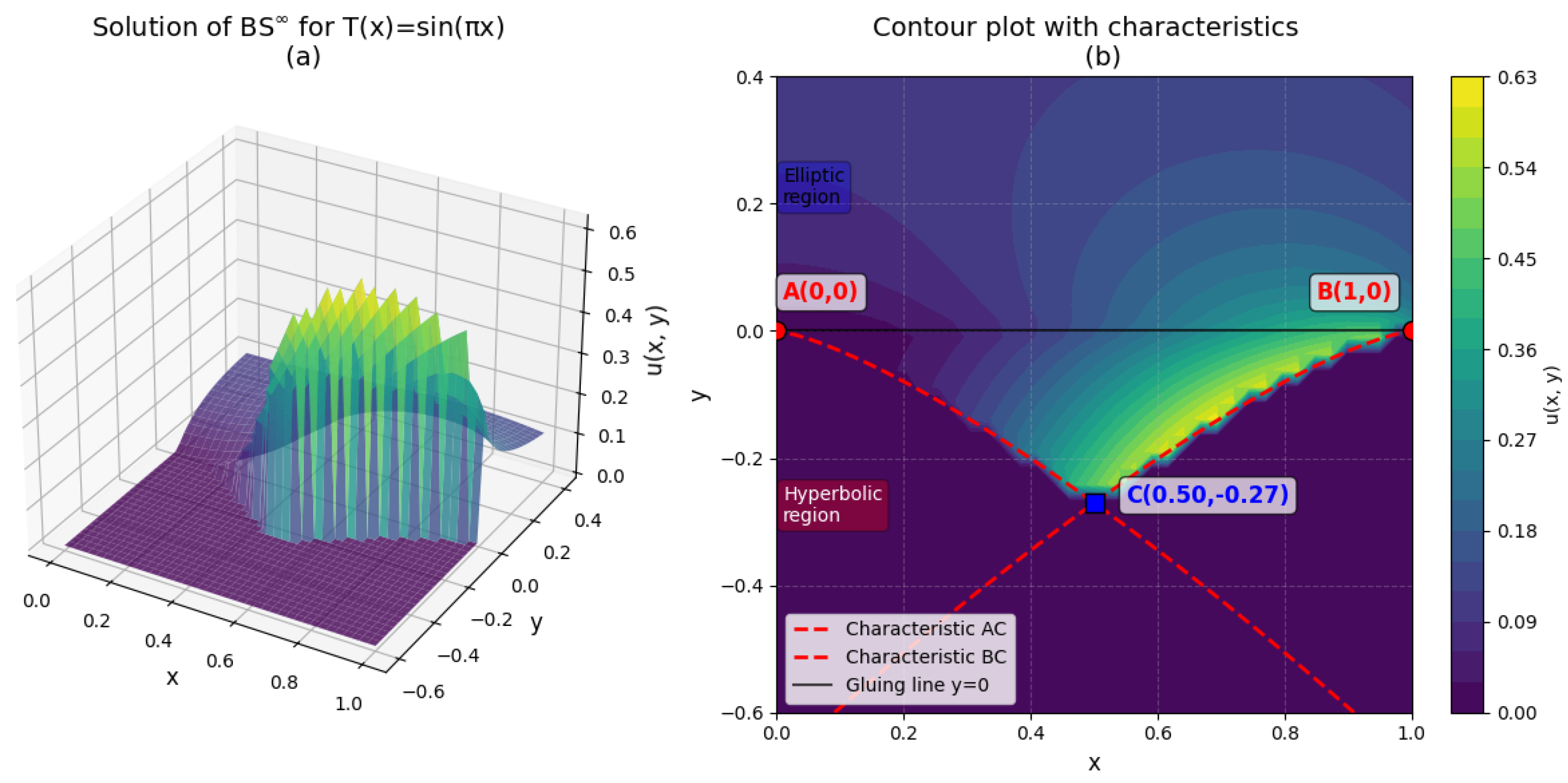
Figure 3 shows the wave pattern, which consists of a 3D surface (Figure 3a) and a contour plot (Figure 3b). They reflect the solution of the Bitsadze-Samarskii type problem. It can be seen that the solution is continuous, the gluing condition is fully satisfied - the contour lines (Figure 3b) from the hyperbolic part smoothly transition into the contour lines of the elliptic part. The mathematical component of the problem is correctly fulfilled.
Let us give a physical interpretation of the Bitsadze-Samarskii type problem. It can be interpreted as a model of wave propagation in an inhomogeneous medium with an abrupt change in properties.
- 1.
- Elliptic region (), a region where the process is stationary or oscillatory without energy transfer over distance. This can be: a cross-section of a waveguide (resonator), where describes the amplitude of a standing wave (for example, mode); a steady-state field (temperature, potential) in a medium where diffusion processes dominate. The solution here oscillates or decays exponentially from the boundary. There are no characteristics - no preferred directions of disturbance propagation. The wave is "trapped" in this region. On the graph, the contour pattern in the upper part (elliptic region) shows the isolines of this stationary field.
- 2.
-
Hyperbolic region (), a region where the process is wave-like, and the equation describes the propagation of disturbances with finite speed. This can be: a region where the medium allows the wave to propagate (for example, open space behind the throat of a waveguide); a model of a dynamic process in time (if y is interpreted as time).There are characteristics along which the wave propagates. In Figure 3b, lines AC and BC are precisely these characteristics. They form the "cone of dependence" of point C. The wave from the elliptic region, penetrating through the boundary , generates in the hyperbolic region two diverging waves traveling along these characteristics.
- 3.
- Gluing line () is a sharp interface between two media with radically different properties: on one side () — a "medium without transfer" (waveguide, diffusive medium); on the other side () — a "medium with transfer" (free space, wave propagation medium). The stationary oscillation in the region () serves as a source for traveling waves in the region . The gluing conditions at are the laws connecting the source field with the radiation generated by it. They ensure that the energy and phase of the wave transition consistently through the boundary.
- 4.
- Note the importance of the nonlocal Bitsadze-Samarskii condition. It not only is an additional condition guaranteeing the uniqueness of the solution but also ensures complete coordination of the solutions in the elliptic and hyperbolic regions. Without this condition, the problem would be underdetermined. This condition also has a physical interpretation - it describes the feedback between standing waves in the elliptic region and traveling waves in the hyperbolic region, and the parameter a plays the role of a feedback coefficient. The nonlocal Bitsadze-Samarskii condition given on the characteristic AC can limit the amplitude of the wave, i.e., the feedback can dampen oscillations. We can see this effect on the contour plot (Figure 3b). Near the characteristic BC we see that the solution has larger values than near the characteristic AC. This is because BC models free wave propagation and therefore can accumulate energy, leading to higher amplitudes (the contour lines on the contour plot near characteristic BC are denser).
The resulting physical picture (using the example ): In the upper elliptic part of Figure 3b () there exists a stationary pattern - a sinusoidal "mode" , fixed at the boundary AB. This mode excites oscillations at the interface . Each point of this boundary becomes a point source for the lower medium (hyperbolic part). Radiation from these sources propagates in the lower region () along the characteristics. As a result, a wave field is formed, shown on the contour plot (Figure 3b) in the lower part: interference of these secondary waves creates a complex pattern, which, however, is completely determined by the original mode and the geometry of the characteristics (AC, BC).
Thus, the Bitsadze-Samarskii type problem mathematically models a complex process of transformation of a standing wave (or stationary field) into a traveling wave upon transition through a critical boundary with feedback, on which the type of the governing differential equation changes.
6. Conclusions
This study investigates a nonlocal boundary value problem of Bitsadze–Samarskii type for a second-kind mixed-type equation in an unbounded domain whose elliptic part is a horizontal half-strip. The main results of the work can be summarized as follows:
A second-kind mixed-type equation with degeneration along the parabolic line, which is the envelope of characteristics, is considered. A problem with a nonlocal condition on the characteristic relating the solution values at different boundary points is studied, generalizing the classical Bitsadze–Samarskii formulation to the case of an unbounded domain and second-kind equations.
Under the condition , the uniqueness of the solution is proved using the extremum principle for the elliptic part and an analysis of the solution behavior at infinity. The existence of the solution is established by the Green’s function method and reduction to a Fredholm integral equation of the second kind. The kernel of the obtained integral equation has a weak singularity, which ensures its solvability within the framework of the Fredholm alternative.
Methods of fractional calculus (Riemann–Liouville derivatives and integrals) are systematically applied, which made it possible to correctly account for the behavior of the solution near the degeneration line. In constructing the Green’s function, properties of special functions—Bessel functions with imaginary argument and the Gauss hypergeometric function—are used, providing an explicit integral representation of the solution.
Numerical visualization of the solution is performed using Python, which confirmed the continuity of the solution, fulfillment of the gluing condition on the line of type change, and consistency between the elliptic and hyperbolic parts. The resulting wave pattern is interpreted as a model of wave propagation in an inhomogeneous medium with an abrupt change in properties at the interface. The elliptic region corresponds to a stationary or oscillatory regime without energy transfer, while the hyperbolic region corresponds to a wave process with finite propagation speed. The nonlocal Bitsadze–Samarskii condition acts as feedback between these regimes, ensuring the physical consistency of the model.
The developed approach can be applied to more general classes of mixed-type equations with fractional derivatives, as well as to problems in domains with more complex geometries. It is of interest to study problems with nonlocal conditions on multiple characteristics, as well as to investigate the asymptotic behavior of solutions as parameters approach critical values. The numerical methods used for visualization can be adapted for solving applied problems in gas dynamics, acoustics, and waveguide theory.
Thus, the work contributes to the theory of boundary value problems for mixed-type equations, expanding the class of studied domains and conditions, offers constructive methods for constructing solutions, and demonstrates their applicability in both theoretical and applied aspects. The research results are supported by rigorous analytical proofs and clear numerical visualization.
Author Contributions
Conceptualization, R.Z. and R.P.; methodology, R.Z.; software, R.P.; validation, A.E., R.Z. and R.P.; formal analysis, A.E.; investigation, A.E., R.Z. and R.P.; writing—original draft preparation, R.Z. and R.P.; writing—review and editing, R.Z. and R. P.; visualization, R.P. All authors have read and agreed to the published version of the manuscript.
Institutional Review Board Statement
Not applicable.
Data Availability Statement
The original contributions presented in this study are included in the article. Further inquiries can be directed to the corresponding author.
Conflicts of Interest
The authors declare no conflicts of interest.
References
- Lavrentiev, M.A.; Bitsadze, A.V. On the problem of equations of mixed type. Reports of the USSR Academy of Sciences 1950, 70, 485–488. [Google Scholar]
- Bers, L. Mathematical aspects of subsonic and transonic gas dynamics; Courier Dover Publications: Mineola, NY, USA, 2016; p. 176. [Google Scholar]
- Frankl, F.I. Selected Works on Gas Dynamics; Nauka: Moscow, Russia, 1973; p. 703. [Google Scholar]
- Chen, Gui-Qiang G. Partial differential equations of mixed type—analysis and applications. Notices of the American Mathematical Society 2023, 70, 8–23. [Google Scholar] [CrossRef]
- Korzhavina, M.V. Tricomi problems for the generalized Tricomi equation in the case of an infinite half-strip. Volzhsky mathematical collection 1971, 8, 114–119. [Google Scholar]
- Korzhavina, M.V. Solution of problem T for the Lavrentiev-Bitsadze equation in an unbounded domain. Differential Equations. Proceedings of Pedagogical Institutes of the RSFSR 1974, 4, 102–108. [Google Scholar]
- Sevost’janov, G. D. Two Tricomi boundary value problems in an unbounded region. Izv. Vyssh. Uchebn. Zaved. Mat. 1967, 1, 95–101. [Google Scholar]
- Fleischer, N.M. On the theory of equations of mixed type in unbounded domains . In Proceedings of the Saratov State University, 1968; Saratov State University: Saratov, Russia; pp. 56–72. [Google Scholar]
- Fleischer, N. M. Boundary value problems for equations of mixed type in the case of unbounded domains. Rev. Roumaine Math. Pures Appl. 1965, 10, 607–613. [Google Scholar]
- Sevostyanov, G.D. Flow of a sonic gas jet around an airfoil. USSR Academy of Sciences. Series of mechanical and liquid gases 1966, 30, 53–59. [Google Scholar]
- Falkovich, S.V. On one case of solving the Tricomi problem. Transonic Gas Flows 1964, 1, 3–8. [Google Scholar]
- Karol, I. L. On a certain boundary value problem for an equation of mixed elliptic-parabolictype. Dokl. Akad. Nauk SSSR 1953, 88, 197–20. [Google Scholar]
- Nakhushev, A. M. Equations of mathematical biology; Vysshaya Shkola: Moscow, Russia, 1995; p. 301. [Google Scholar]
- Bitsadze, A.V.; Samarskii, A.A. Some elementary generalizations of linear elliptic boundary value problems. Dokl. Akad. Nauk SSSR 1969, 185, 739–740. [Google Scholar]
- Nakhushev, A.M. Fractional calculus and its applications; FIZMATLIT: Moscow, Russia, 2003; p. 272. [Google Scholar]
- Smirnov, M. M. Equations of mixed type. 51; American Mathematical Soc.: Providence, USA, 1978; p. 232. [Google Scholar]
- Bitsadze, A.V. Equations of the mixed type; Elsevier: Amsterdam, Netherlands, 2014. [Google Scholar]
- Sabitov, K. On the Theory of Mixed-Type Equations; LitRes: Moscow, Russia, 2016. [Google Scholar]
- Ezaova, A. G. Unique Solvability of a Bitsadze-Samarskiy Type Problem for Equations with Disontinuous Coefficient. Vladikavkaz Math. J. 2018, 20, 50–58. [Google Scholar]
- Mirsaburov, M.; Makulbay, A.B.; Mirsaburova, G. M. A combined problem with local and nonlocal conditions for a class of mixed-type equations. Bulletin of the Karaganda University. Mathematics Series 2025, 118, 163–176. [Google Scholar] [CrossRef]
- Repin, O.A.; Kumykova, S.K. On a boundary value problem with shift for an equation of mixed type in an unbounded domain. Differential Equations 2012, 48, 1127–1136. [Google Scholar] [CrossRef]
- Zunnunov, R.T.; Ergashev, A.A. The problem with shift for an equation of mixed type of the second kind in an unbounded domain. Vestnik KRAUNC. Fiz.-Mat. Nauki 2016, 1(12), 26–31. [Google Scholar] [CrossRef] [PubMed]
- Khairullin, R.S. Boundary value problems for a mixed-type equation of the second kind; Kazan University Publishing House: Kazan, Russia, 2020; p. 356. [Google Scholar]
- Muminov, F.M.; Muminov, S.F. About One Nonlocal Boundary Value Problem for a Mixed Type Equation. Central Asian journal of mathematical theory and computer sciences 2021, 2, 29–32. [Google Scholar]
- Zunnunov, R.T. A Problem with Shiff for Mixed-Type Equation in Domain, the Elliptical Part of Which Is a Horizontal Strip. Lobachevskii journal of mathematics 2023, 44, 4410–4417. [Google Scholar] [CrossRef]
- Turmetov, B.Kh; Kadirkulov, B.J. On a problem for nonlocal mixed-type fractional order equation with degeneration. Chaos, Solitons & Fractals 2021, 146, 110835. [Google Scholar]
- Ruziev, M.G.; Zunnunov, R.T. On a nonlocal problem for a mixed-type equation with a partial fractional Riemann-Liouville derivative. Fractal and Fractional 2022, 6(2), 1–8. [Google Scholar] [CrossRef]
- Ruziev, M.H; Parovik, R.I; Zunnunov, R.T; Yuldasheva, N. Non Local Problems for the Fractional Order Diffusion Equation and the Degenerate Hyperbolic Equation. Fractal Fract. 2024, 8, 538. [Google Scholar] [CrossRef]
- Kilbas, A.A.; Srivastava, H.M.; Trujillo, J.J. Theory and applications of fractional differential equations; Elsevier: Amsterdam, Netherlands, 2006. [Google Scholar]
- Bitsadze, A.V. Boundary value problems for second order elliptic equations; Elsevier: Amsterdam, Netherlands, 2012; Vol. 5. [Google Scholar]
- Lebedev, N.N. Special functions and their applications; Prentic-Hall: London, UK, 1965; p. 322. [Google Scholar]
- Shaw, Z.A. Learn Python the Hard Way; Addison-Wesley Professional: Carrollton, USA, 2024. [Google Scholar]
Figure 1.
Characteristic triangle in the hyperbolic part.
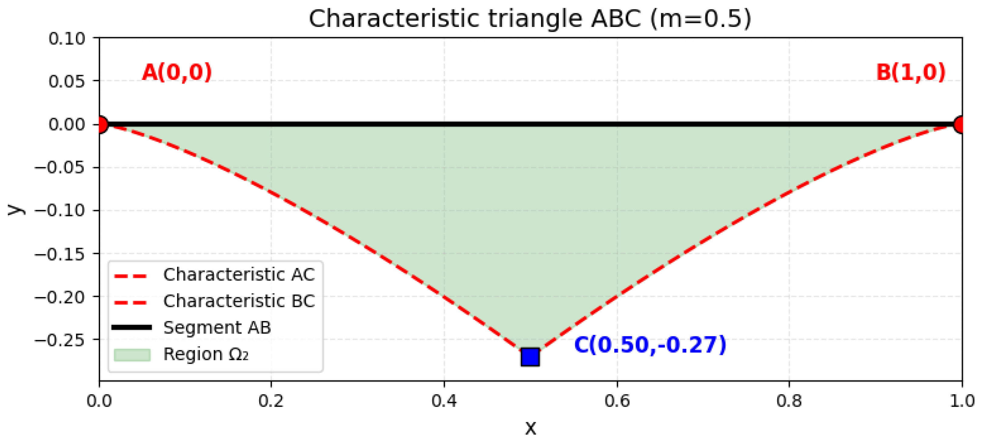
Figure 2.
Graphs: (a) - ; (b) - .
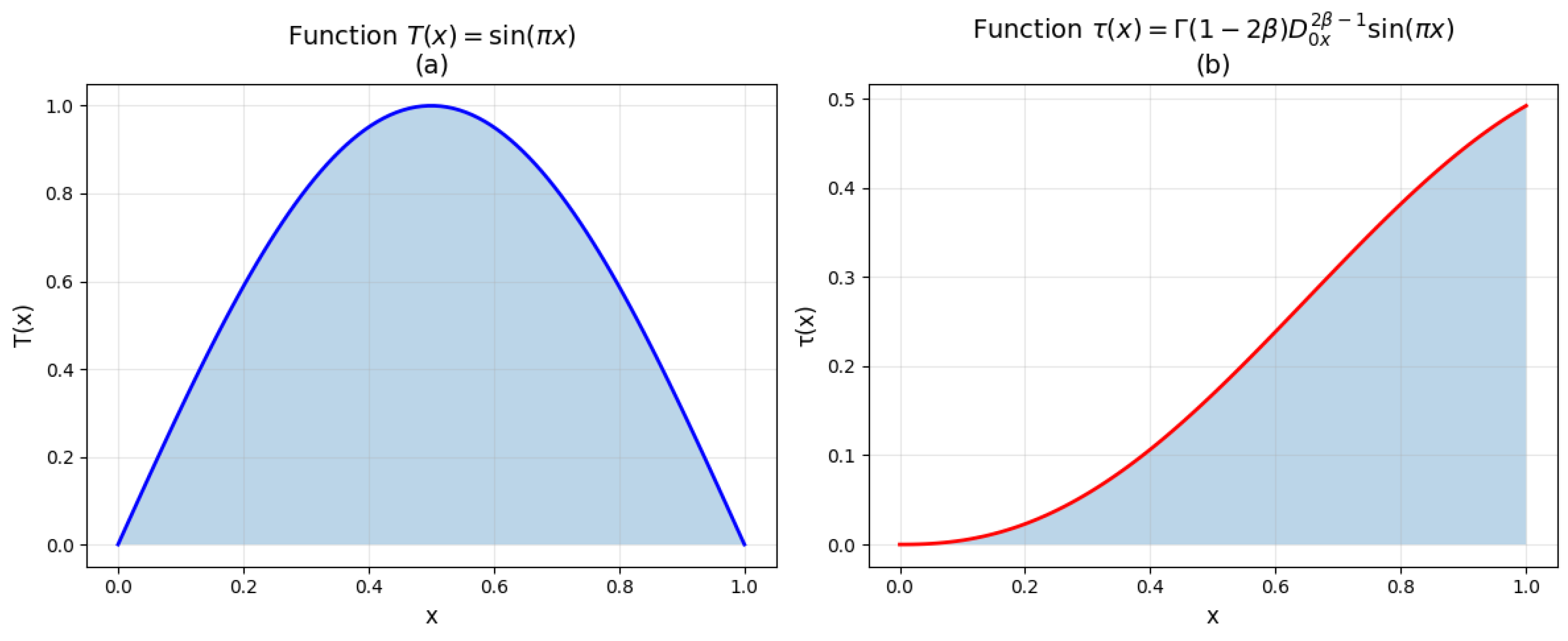
Figure 3.
Wave pattern: (a) - 3D plot of the solution to the BS∞ problem; (b) - contour plot of the solution to the BS∞ problem.
Figure 3.
Wave pattern: (a) - 3D plot of the solution to the BS∞ problem; (b) - contour plot of the solution to the BS∞ problem.
Disclaimer/Publisher’s Note: The statements, opinions and data contained in all publications are solely those of the individual author(s) and contributor(s) and not of MDPI and/or the editor(s). MDPI and/or the editor(s) disclaim responsibility for any injury to people or property resulting from any ideas, methods, instructions or products referred to in the content. |
© 2025 by the authors. Licensee MDPI, Basel, Switzerland. This article is an open access article distributed under the terms and conditions of the Creative Commons Attribution (CC BY) license (http://creativecommons.org/licenses/by/4.0/).
Copyright: This open access article is published under a Creative Commons CC BY 4.0 license, which permit the free download, distribution, and reuse, provided that the author and preprint are cited in any reuse.


