A Low-Cost, Open-Source Snow Sensing Station Design for Increasing the Spatial Distribution of Snow Observations

1. Introduction

Snow is a critical component of water resources management on a global scale, with snowmelt supplying water to approximately one-billion people [1]. Snowmelt can be a major contributor to the total runoff in a watershed. In the western United States, about 53% of the total runoff is attributable to snow [2]. This can be even more pronounced in some western states, such as Utah, where 98-99% of total stream discharge originates from snow [3]. Understanding the role of snow in hydrologic processes is critical for managing water resources in these watersheds. Snow hydrologists are primarily interested in understanding the accumulation and ablation processes that ultimately affect the amount of water in a snowpack and how it will influence streamflow. Hydrologists approach this problem using both measurements and modeling.

Physically based hydrologic models, such as the Utah Energy Balance model [4], can help predict snow processes by using observable data and mathematical equations that approximate physical processes occurring within the hydrologic system. By understanding the phenomena that drive snow processes, we can make more meaningful environmental measurements at sites of interest that can be used to predict streamflow from snowmelt [5]. In snow hydrology, the physical processes driving the transport of water are mass and energy flux into and out of a snowpack, with the snowpack acting as the changing storage for both mass and energy [6]. Mass fluxes into a snowpack primarily consist of new snowfall but can also include rain on snow events, vapor deposition, and wind deposition [7,8,9]. Mass fluxes out of a snowpack consist mostly of melting but can include sublimation and wind scour [7,10].

Energy fluxes into and out of a snowpack are primarily transfers of heat, which is critical in predicting snowmelt timing and runoff rates [11]. These phenomena include electromagnetic radiative fluxes, conductive fluxes from the ground, sensible and latent heat fluxes from rain, and sensible and latent turbulent diffusion from the air above a snowpack [12]. Understanding how these processes influence snow hydrology will only become more important as the consequences of human-caused climate change become more apparent [13].

Automated collection of environmental measurements that characterize these important variables at a site of interest can enable hydrologists to make more accurate predictions of snow accumulation and melt processes [15]. In the western United States where snow is a primary driver of hydrology, the most extensive network of snow measuring stations is operated by the United States Department of Agriculture’s (USDA) Natural Resource Conservation Service (NRCS). This telemetry system, named SNOTEL, includes around 900 stations [15] that measure many of the environmental variables of interest, including snow water equivalent (SWE), which is an estimate of the depth of water in a snowpack (i.e., the equivalent depth of water that would exist if a vertical column of snow were melted to its liquid state) [16].

While the data collected by the SNOTEL network is generally of high quality and is used extensively to support modeling and water resources management, the SNOTEL network has limitations. Given the broad spatial distribution of the network in the western U.S., most watersheds have a small number of stations located within or immediately adjacent to the watershed, and many have none [17]. Despite this, SNOTEL stations are meant to be representative of the conditions for an entire watershed and are installed with the intention to predict runoff within watersheds containing significant agricultural activity. The USDA has set guidelines in the National Engineering Handbook for SNOTEL site selection that inherently bias the measurements made across the network [18,19]. Viable sites must have open sky exposure, easy access, flat terrain, and low wind impact. Stations are also generally installed at elevations and locations that receive and hold snow well into the spring season. They are also located in areas meant to be representative of the basin, but this is secondary to the accessibility and terrain requirements.

While these criteria may be suitable for estimating potential runoff to meet the needs of agricultural water managers, they can leave gaps for hydrologists that want to understand how variables such as terrain, tree canopies, vegetation, slope, etc. can affect snow accumulation and melt. Data characterizing these variables used as forcing for process-based models can, therefore, be spatially limited when using SNOTEL alone [20]. While expanding the existing SNOTEL network with additional stations might help alleviate the inherent bias in SNOTEL data, cost is an obvious limitation. SNOTEL stations can cost around $30,000 U.S. to install, which can be attributed to the extensive hardware used for measuring variables such as SWE and precipitation, which require a snow pillow and precipitation gauge, as well as high-end data logging, communication devices, and mounting platforms. There is a need for lower cost alternatives for expanding existing snow measurement networks beyond SNOTEL to include more measurements made at sites conducive to snowpack variability by selecting lower-cost hardware [5].

In recent years, there has been a movement within the scientific research community for inexpensive and open-source monitoring hardware and software that make it easier to collect environmental sensor data in more locations. Various authors discuss advances in using open-source microcontrollers for research data collection [21,22,23,24]. Pohl et al. [25] describe a platform they developed titled SnoMoS, which is a low-cost sensor network for collecting snow data. While this study describes the sensors they selected and how spatially variable snow data can be, there is no discussion of the selection or construction of their datalogger, where to find supporting code, and how to wire, configure, and construct the station. Thus, reusability of their results is low, representing a knowledge gap in implementing lower-cost sensing for snow measurements.

Abdelal and Al-Hmoud [26] created a modular Internet of Things (IoT) based hydrological monitoring platform using low-cost and low-power systems called the HydroMon3. This, however, was not tested for winter conditions, and there is an absence of discussion around quantifying power requirements. They were also not able to demonstrate an implementation with solar panels because of vandalism concerns. Hund et al. [21] also developed a low-cost hydrological monitoring system based on the Arduino board called the Ecohydro Logger. This data logging system was likewise not designed for snow hydrology purposes, and there is no discussion on power requirements and power design. Limited published work exists describing use of open-source microcontrollers to monitor snow hydrology, and there is also a lack of clear procedures for the hardware and software design of these monitoring platforms. Properly using open-source microcontrollers as dataloggers for environmental monitoring can prove difficult without education or training in electrical engineering. This paper seeks to address these concerns, specifically within the snow hydrology community.

While low-cost systems can be deployed to enable autonomous measurements using a variety of sensors and can store data within local memory at the datalogger station, integrating telemetry components that enable communicating data, potentially in near real-time, from a monitoring station to a data management system can be challenging. Lack of data communication via telemetry causes delays in retrieving data that may limit how the data can be used [27] and may also lead to permanent data loss if the datalogger’s local memory becomes compromised or corrupted or if a sensor, datalogger, or program malfunctions between site visits. These factors then impact users’ ability to access the data if the data was intended to be published. Thus, solving these issues is imperative in developing robust and reliable low-cost sensing stations. Many commercially available, purpose-built dataloggers already have integrated hardware and software enabling data communications—e.g., the Campbell Scientific CR350 (https://www.campbellsci.com/cr350) or the Onset MicroRX Station (https://www.onsetcomp.com/products/data-loggers/rx2100). Proprietary systems are engineered to be robust in enabling reliable communications with remote monitoring stations. However, they are expensive, with dataloggers costing as much as $1,000 to $1,500 U.S. or more and communication peripherals costing sometimes on the order of $500 to $1,000 U.S., which has driven many scientists and practitioners to consider less expensive alternatives.

Adding telemetry to low-cost dataloggers (e.g., those based on inexpensive Arduino microcontrollers) is an obvious extension of low-cost sensing, but the level of component integration and engineering present in commercial dataloggers is lacking for low-cost dataloggers, which means that successful applications require some electronics development expertise because most Arduinos do not have integrated communication capabilities. In some low-cost sensing applications reported in the literature, data collection stations lacked telemetry components entirely and required visiting the site to download the data [25]. Other researchers have made efforts to develop methods for communicating data using radio frequency (RF) technologies integrated with Arduino-based dataloggers. For example, Mahbub [28] demonstrated a use case with an Arduino Uno and a separate 2.4 GHz radio module, the nRF24L01 by Nordic Semiconductor [29], but this module can only transmit about 100 meters, and the case study was for wirelessly controlling light emitting diodes and motors. Nedelkovski [30] used the same RF module to develop an at-home miniature weather station that could collect and transmit the data through an Arduino, but likewise transmission distance was limited, and data only had to be aggregated from one station. Sadler et al. [31] developed a method of transmitting data using Arduinos with a separate cellular radio module, but their study did not address transmitting data out of areas without cellular connection. In other study applications, telemetry components were reported, but without sufficient detail to enable building from or reusing their methods—especially for potential users who lack electrical engineering experience [32].

Given the need for enhanced snow measurements and the limitations of previous lower-cost solutions, the goal of this paper is to describe an open-source, lower-cost snow sensing system designed for collecting high temporal resolution measurements of environmental variables relevant to modeling snow. This sensing system is made up of a suite of scientific grade sensors paired with an Arduino-based datalogger and off-the-shelf electrical components assembled in a package that is simple to deploy using multiple potential deployment platforms. We demonstrate using both cellular and 900 MHz spread spectrum radio telemetry to enable near real-time data communications, formalizing systems for wirelessly communicating observations to downstream networking and cyberinfrastructure designed to accept those measurements and make them available on the Internet. Specific contributions of this paper include the station design, open-source code for logging and transmitting data, procedures and communication protocols for telemetry using multiple radio modules and monitoring network architectures, and an open GitHub repository that provides practical information on the selection of sensors, construction/deployment of a snow sensing station, detailed wiring instructions, and open-source code for integrating sensors with an open-source datalogger. The station design presented here can be used to deploy lower-cost snow sensing networks that can be repeated by other researchers and adjusted to their needs. We demonstrated station design, integration, and operation through a multi-station case study deployment near the Tony Grove Ranger Station (TGRS) SNOTEL station in northern Utah, USA.

2. Materials and Methods

2.1. Requirements and Design Considerations

The specific requirements we identified for successful deployment of low-cost snow sensing stations are as follows:

• Must collect environmental measurements that facilitate the modeling and prediction of snow hydrology processes.
• Must support common sensor inputs to facilitate use of research grade sensors and to enable further development of these stations with sensors other than those listed in this final design.
• Must collect data at regular intervals and record observations along with their timestamps in local storage on the datalogger.
• Must be constructed using easily available, off-the-shelf components that are available locally or online.
• Assembly and deployment of the station must be possible by anyone with the proper tools.
• Must be deployable on a variety of terrains, such as slopes and under tree canopies.
• Must be autonomously powered and configurable to use a variety of power sources and systems appropriate for selected deployment locations.
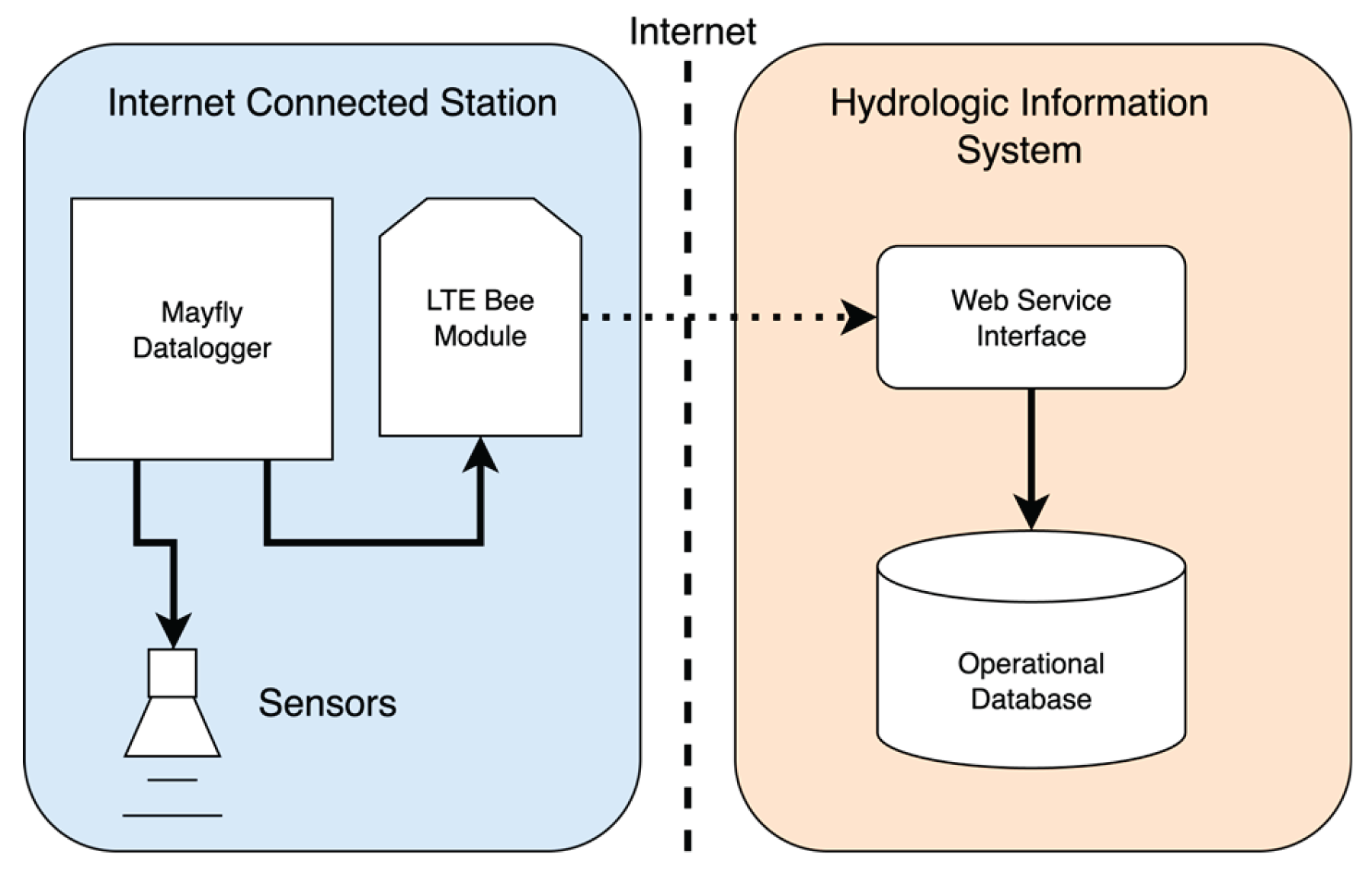
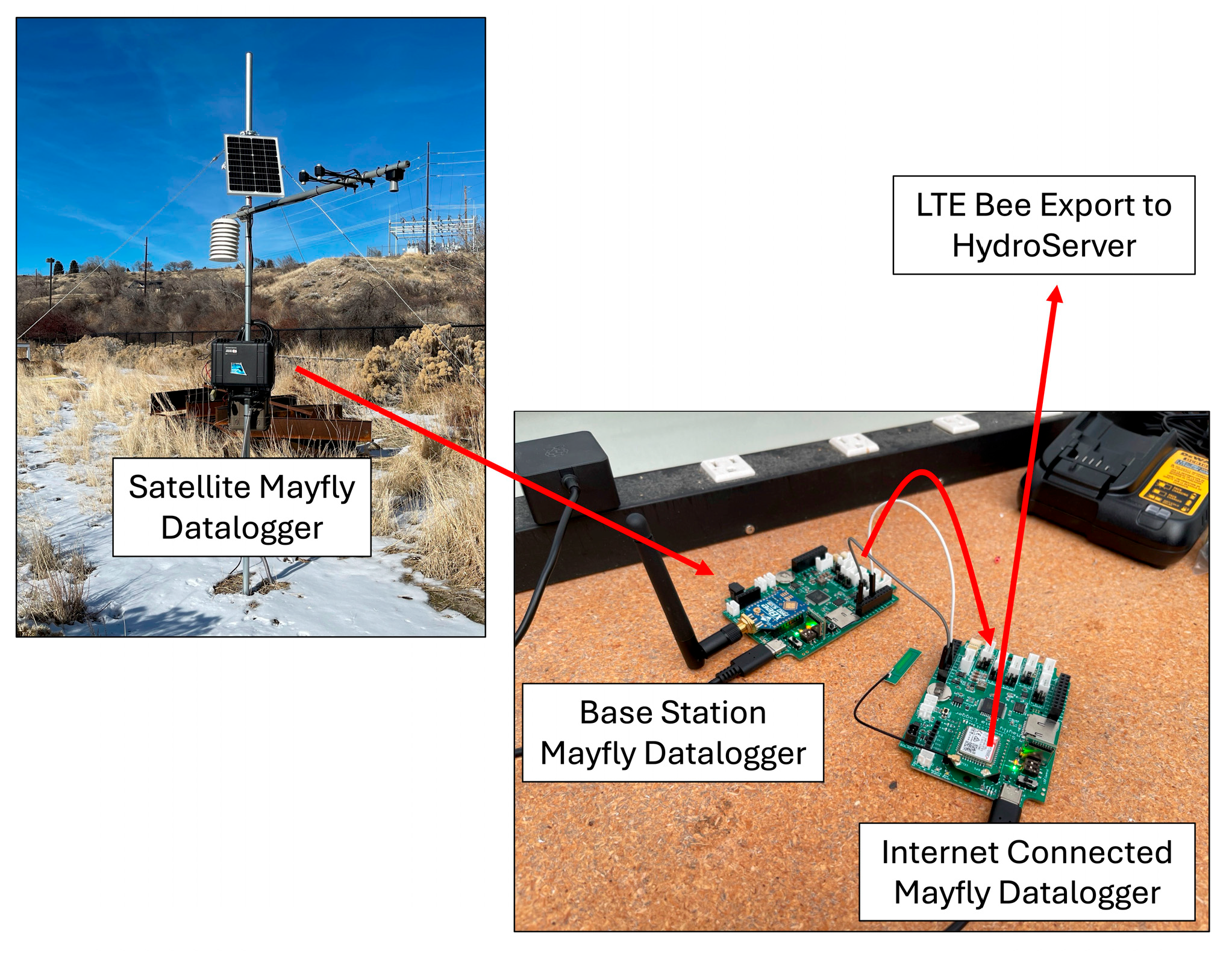
• Must be capable of connecting to the Internet directly with cellular data coverage or by wirelessly sending data to another station that has an Internet connection.
• Must be capable of transmitting data and integrating with existing radio telemetry systems (e.g., stations must be capable of joining a radio network with other, existing stations).
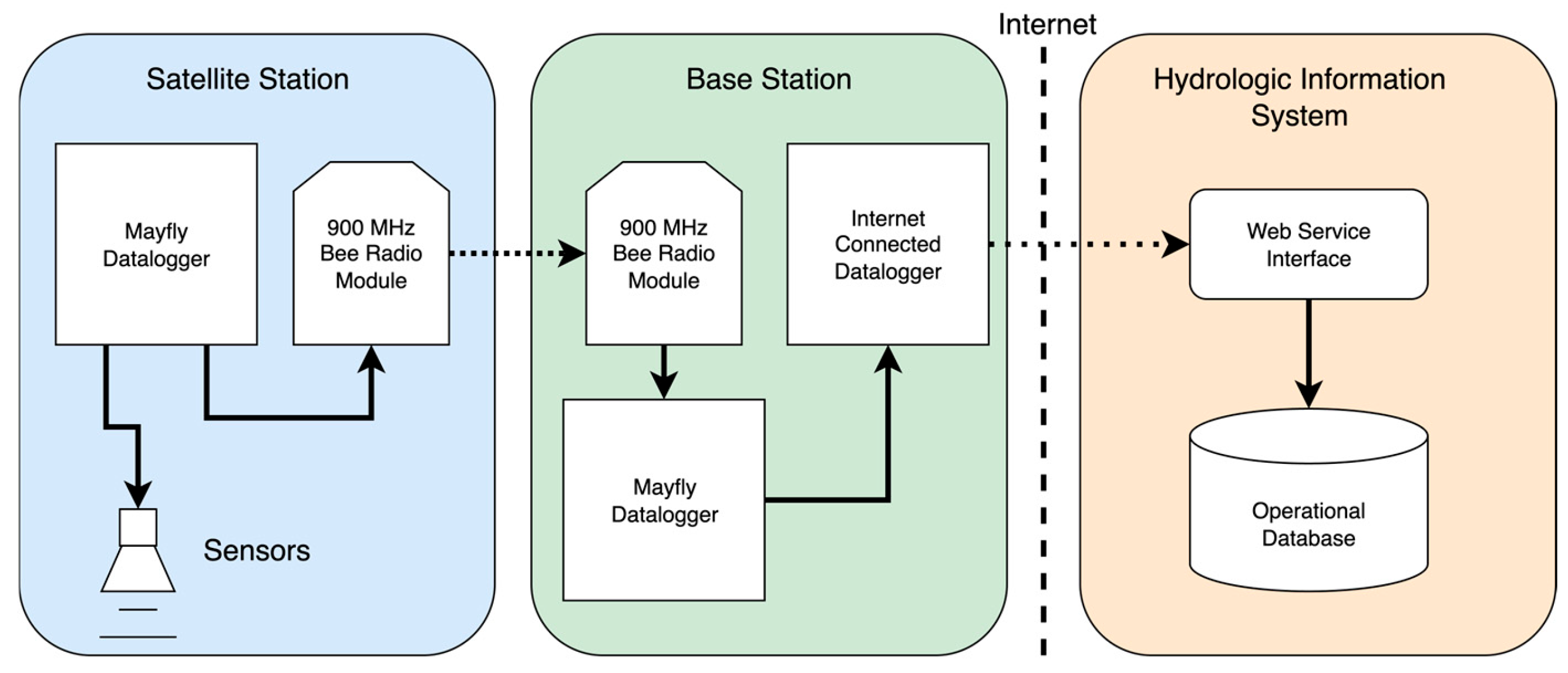
• Must be capable of participating in hybrid networks that mix radio technologies (e.g., multiple stations communicating data using 900 MHz spread-spectrum radios to a station that has a cellular Internet connection).
• Must be capable of manual data downloads or integration with a Hydrologic Information System (HIS) for real-time delivery of data to an operational system that enables storage, management, and sharing of the data.

In the following sections we describe the snow sensing station architecture, sensing and data logging hardware design, required code, power systems, communications and telemetry, and deployment platform. Each of the requirements above are addressed and discussed in these sections. At the time of this writing, the total cost of a monitoring station according to this design was approximately $4,142 when using off-the shelf electronic components and mounting hardware or up to $9,182 if using more expensive (but potentially higher quality) power and mounting components purchased from a company like Campbell Scientific (https://www.campbellsci.com/). Costs here and throughout this paper are expressed in U.S. dollars. In the project’s GitHub repository (see Software and Data Availability Section), we provide two spreadsheets that list each individual component required, where those components can be sourced, and the cost of the component at the time of this writing. In the sections that follow, we have broken down the costs of each of the components within major categories (e.g., sensors, datalogger, power, communications, deployment platform, etc.).

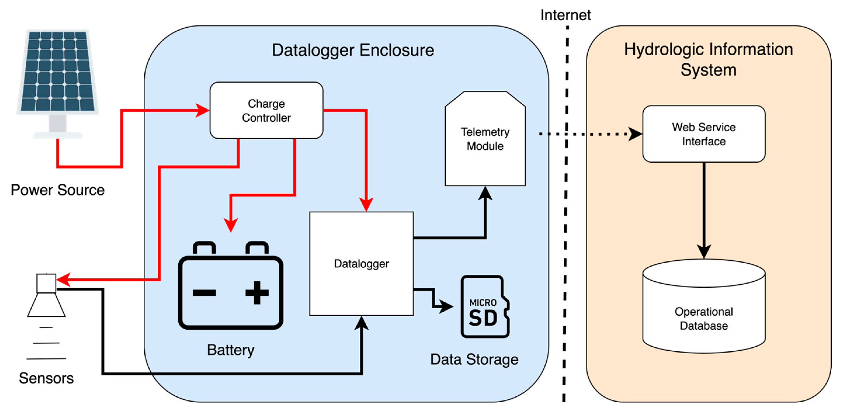
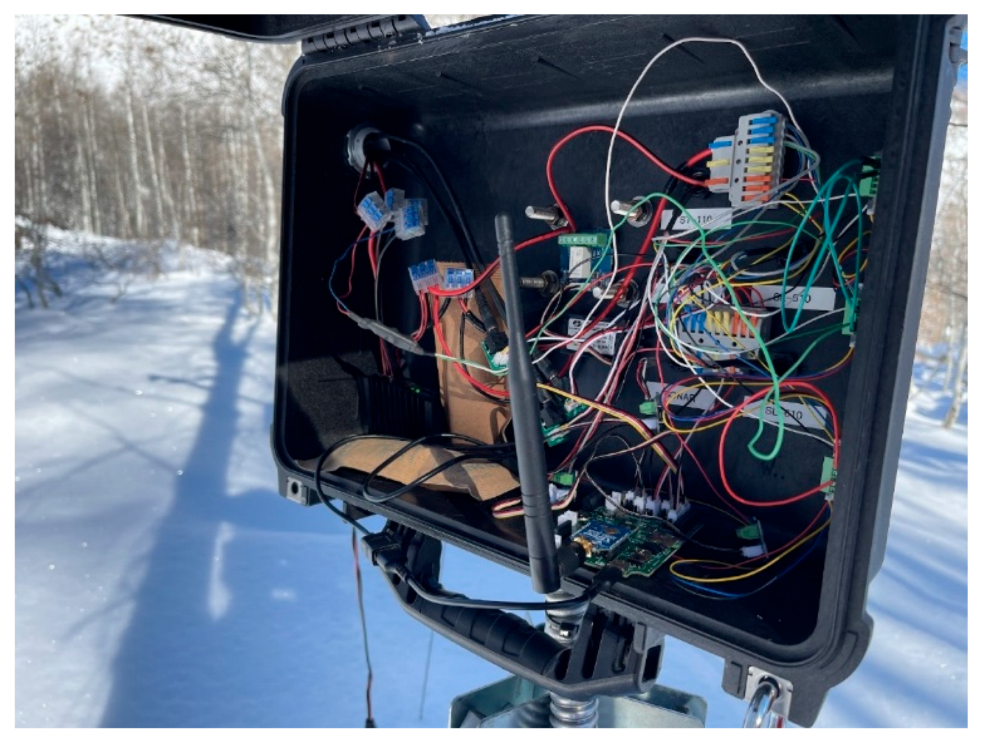
2.2. Station Architecture, Sensing, and Data Logging Hardware Design

The snow sensing station components follow the layout shown in Figure 1. A datalogger is housed in a weatherproof enclosure that handles the measurement, collection, and recording of data from a suite of environmental sensors. Data is recorded on a secure digital (SD) storage card and can be transferred over wireless telemetry modules if those are added to a station as described in Section 2.5. A battery, either in the same or in a separate enclosure, powers the datalogger and any other necessary peripherals through a charge controller, which also supplies recharge to the battery through a power source such as a solar panel. Each of these components and other necessary peripherals are discussed in the following subsections.

2.2.1. Sensors

Environmental variables useful as input data for snow modelers help quantify the amount of snow present and the energy exchanges that occur between a snowpack and its surroundings. This is necessary to enable prediction of the rate and timing of snowmelt, as well as the volume of subsurface flows that occur during spring snowmelt. Primary variables include, but are not limited to, snow depth, net radiative fluxes, air and soil temperatures, soil matric potential, and soil volumetric water content. This station design addresses the first requirement in Section 2.1 by measuring these variables with the following selection of sensors, the costs of which are listed in Table 1. While a major objective was to design a lower-cost snow sensing station, we opted for reasonably priced, but still research-grade sensors to ensure that lowering costs did not sacrifice the quality of the observations. Each of these sensors is described in more detail in Appendix A.

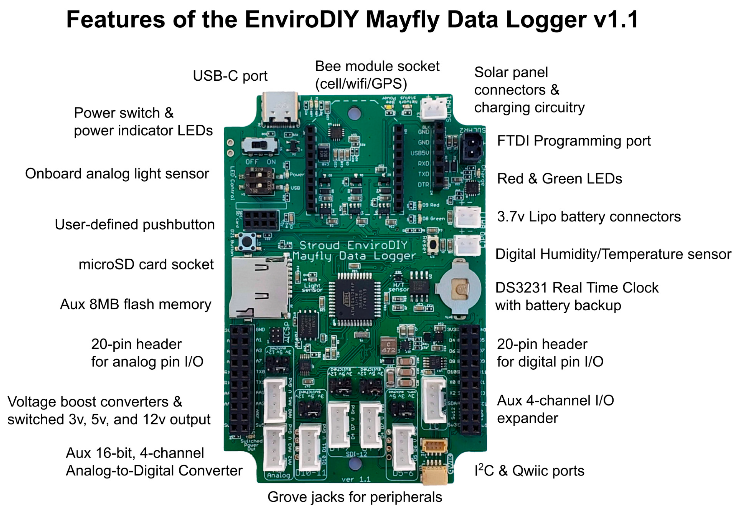
2.2.2. Datalogger

Open-source microcontrollers provide an opportunity for low-cost data logging and sensor integration when compared to scientific grade dataloggers like those from Campbell Scientific that can cost well over $1,500. The Arduino Uno is an affordable microcontroller but does not meet requirement three from the design considerations as it lacks a real-time clock and memory storage capabilities. It also lacks dedicated pins for adding communication modules, secure wiring attachments to avoid sensor wires losing connection to their header pins, and switched power. These could be added as peripherals, driving up the cost and required integration effort; however, the Stroud Water Research Center has already developed an inexpensive, Arduino-based Mayfly datalogger that addresses these limitations and is compatible with the Arduino Interactive Development Environment (IDE) and Arduino code libraries [33].

The Mayfly datalogger includes a real-time clock and SD card reader, which addresses requirement three, multiple sensor type connections that help meet requirement two, variable voltage switched power, an on-board 16-bit analog-to-digital converter (ADC) which has higher resolution than the Arduino Uno’s 10-bit ADC, and Qwiic ports for easily expanding inter-integrated circuit (I2C) connections. The Mayfly also has a built-in header for plugging in Bee radio telemetry modules, which simplifies adding RF communication to a Mayfly datalogger. Many wireless communication modules from various companies and research groups use the Bee footprint and protocols (e.g., Digi, EnviroDIY, Seeed Studio), which means that the same header can be used for cellular, 900 MHz spread-spectrum, LoRa, or other types of RF communications, which addresses requirements eight through ten. Specifics of communication protocols, networking, and telemetry are discussed in Section 2.5. Figure 2 shows the Mayfly datalogger and many of its listed features from the EnviroDIY website [34] where these boards can be purchased.

While the Mayfly’s added hardware functionality is a major benefit for low-cost data logging, the groundwork done by the Stroud Water Research Center in developing software for the Mayfly is another reason to select this board for snow sensing. They have developed an open-source Arduino library called ModularSensors [35] that handles managing power to sensors, making measurements, recording data values to the SD card, and publishing those data points to the Internet, which helps fulfill requirement three and eight through ten. Some of the code had to be customized to properly deploy snow sensing stations (see Section 2.3) and to enhance the telemetry networking and data publication capabilities.

One shortcoming of the Mayfly we had to address is that it lacks the number of analog inputs required by the sensors we selected, including the four radiometers and one air temperature sensor. The Mayfly alone includes four channels for its 16-bit ADC, but these sensors require a total of nine. Using the Adafruit ADS1115 [36] ADC and their Qwiic port connections, extra ADCs can be daisy-chained to the Mayfly to accommodate more analog measurements. These ADCs have programmable gain amplifiers to get higher resolution readings on small voltages and are solderable for use on a development board.

Table 2 lists the total cost for the datalogger and communication peripherals. Note that the antenna and radio module are only used for networking communications, which is not necessary for operating a station unless data telemetry is required. Those items are discussed in further detail in Section 2.5.

2.3. Code

The ModularSensors library is a comprehensive Arduino library that manages power and the timing, measurement, and logging of data on a Mayfly datalogger. It is open source, freely downloadable, and editable. While the source code already includes interoperability with a wide range of environmental sensors and examples of how to use the ModularSensors library in programming a Mayfly, we made adjustments in both the ModularSensors code and the example Arduino sketches for logging data to accommodate the sensors and power deployment options we selected for our station design.

The most notable change in code was the addition of code for sensors that were not included in the original library. The MaxBotix MB7374 sonar sensor was already included in the source code, but none of the other sensors we selected were. A small adjustment was made to the MaxBotix code to allow for measurements on sloped surfaces. The Apogee pyranometer source code was created based on the existing Apogee SQ-212 files within ModularSensors that follow a similar procedure for recording analog measurements and adjusting them based on calibration factors. The longwave radiation sensors were added based on the code for the shortwave radiation sensors because they similarly output differential thermopile analog measurements, but that code also included taking thermistor measurements to get temperature and calculate the final longwave radiation measurement. The air temperature sensor is a single-ended analog output that operates effectively like the thermistor on the longwave radiation sensors, so its source code was developed from that. Source code for the Meter Teros 11 sensor was already part of the ModularSensors library, so small adjustments were made to that code to accommodate the extra measurement that the Teros 12 makes as well as to accommodate multiple SDI-12 sensors connected to the same datalogger port.

Section 2.4 describes power considerations for the snow station design, which include managing the power supplied to the heaters that keep the pyranometers and pyrgeometers free of snow and ice. Code functionality was added to the Mayfly data logging sketch to control the power to these heaters based on a time during a logging interval. This code supplies or cuts power to the heaters based on user designated times.

As part of the development and testing of the snow sensing stations, utility Arduino sketches were created to facilitate various tasks such as testing sensors for functionality, testing sensor performance using the ModularSensors library, reading data from SD cards into the Arduino IDE serial monitor, and measuring and logging power requirements for a station. These utility sketches are included in the GitHub repository for this project.

The Arduino sketch used for logging snow station data on the Mayfly follows the general structure of EnviroDIY’s ModularSensors examples by first including the various libraries needed to function. Because snow stations also have telemetry functionality, this feature is also turned on or off at the beginning of the sketch depending on whether it will be used or not. Various variables used throughout the sketch are then defined, followed by the up-front work needed to set up each sensor, such as specifying calibration factors, sensor installation heights, sensor names, etc. In the Mayfly’s setup function, pin modes are set as well as clock communication rates, and certain microcontroller processes are started such as serial communication settings and telemetry settings if those are incorporated. In the loop function, the sketch cycles through checking whether the radiometer heaters need to be turned on and whether it is time to measure and log data. The full data logging sketches are contained within the “code” folder in the project GitHub repository.

2.4. Power

The snow stations were designed to operate with a variety of power supply options based on their exposure to the sun to fulfill requirement seven. Variety in power supply options includes variety in battery sizes, solar panels, and charge controllers. The availability and selection of these components are discussed in this section as well as the addition of a buck power converter and a power relay to the final design. Table 3 summarizes the costs of power components using high quality solar panels and charge controllers purchased from Campbell Scientific. Note that the wattage for the solar panel is only 10 watts compared to that in Table 4, which summarizes the costs for solar panels and charge controllers easily sourced online. Costs in Table 3 and Table 4 are provided separately to demonstrate potential savings by sourcing power components via common online outlets.

2.4.1. Power Relay

The heaters on the Apogee radiometers are the largest source of power draw in this design, requiring about 80 mA to run, whereas the system idles at about 20 mA when not taking measurements or powering the heaters and about 30 mA when logging data. To control the power to the heaters, a latching relay is used. A latching relay is a device that can control power by supplying a rising or falling voltage to coils that will then open or close a circuit and retain that position by hooking and unhooking a plastic latch. Seeed Studios sells a $7.60 2-coil latching relay that has a Grove terminal for connecting to other Grove ports like the ports on the Mayfly [37]. With this relay, all stations can optionally control the power supply to the sensor heaters using code. This helps extend battery life and reduce power requirements.

2.4.2. Battery

Properly sizing the battery that powers the snow station helps ensure operation time, especially where solar recharge may be inadequate. The battery must supply a high enough voltage for the electronics to operate, and it needs enough capacity for the station to operate with or without solar recharge (depending on deployment location). Battery voltage is determined based on the highest voltage demand of the system. In this design, the Mayfly datalogger operates at 5 volts. The Mayfly has the capacity to supply switched power to the sensors at 3.3 volts, 5 volts, or even 12 volts, which covers all the sensors for the duration of their measurements which lasts less than a minute.

The Apogee radiometers, however, have heaters that require sustained 12-volt power. While the Mayfly can supply switched power to sensors, it was not designed to supply sustained power for long periods of time to sensor heaters, and the required power draw would be strenuous for the microcontroller [38]. Therefore, the heaters are connected to the 12-volt battery through the latching power relay, and a buck converter is used to lower the 12-volt battery supply to the 5-volt power required by the Mayfly.

Equation 1 is used to calculate the battery capacity needed for a station, in amp-hours:

$$BatteryCapacity={\displaystyle \frac{Load\ast Time}{Efficiency}}$$

(1)

where Battery Capacity is the minimum amp-hour rating of a battery; Efficiency is the battery discharge efficiency in cold weather conditions, which differs from the recharge efficiency depending on the battery type; Load is the average current draw in amps of the system over every duty cycle, which is the entire set of functions and processes completed by the microcontroller and peripherals repeated during each logging interval; and Time is the hours of operation without solar recharge or swapping batteries. In general, this equation describes how the battery capacity needed is the load taken over time and adjusted based on how much capacity the battery loses in cold weather.

The load is determined by measuring the amperage drawn from the positive terminal of a battery to the station peripherals using an amp-meter or power sensor. To properly size a battery using these tools, the station must be assembled and operating as expected. After assembling a station and powering it with any 12-volt battery, a power sensor or an amp-meter can be added in series to measure the current being drawn from the positive terminal of the battery. Measurements must be taken frequently enough to capture all the changes in current demand throughout a duty cycle. The load is then calculated by averaging each measurement over the duty cycle (Equation 2):

$$Load=\sum p_n\ast I_n$$

(2)

where p_n is the fraction of time in the duty cycle that any process n is operating, and I_n is the current draw of process n. The required battery capacity is also dependent on how long the battery needs to last without being recharged. If it is a station with no intention of solar recharge (e.g., a station deployed on a north facing slope under a conifer canopy), the required capacity determines how long one can go without making a trip to swap the battery. If there is anticipated solar recharge, required capacity is how long the battery must last during periods of snow or heavily overcast conditions, which may last several days during winter months.

Efficiency of batteries in cold weather conditions depends on battery chemistry. For stations that will have no solar recharge, a lithium-ion battery is preferable because of its higher discharge efficiency [39], which can near 100% in cold weather [40]. For stations with solar recharge, a sealed lead-acid (SLA) battery is preferred for its lower cost and higher recharge efficiency, but it does have significant reduction in discharge efficiency, particularly when discharging quickly, with an efficiency between 60-80% at -20 degrees Celsius [40].

2.4.3. Charge Controller

A charge controller regulates power supplied from a solar panel to a battery, helping to avoid damage from overcharging. Some also help stop current being drawn from a battery if the battery voltage drops below the rated voltage. The charge controller must be capable of outputting 12 volts for the sensor heaters. For these stations, we tested two different charge controllers. The first is the Campbell Scientific CH150, which can output 12 volts and charge a 12-volt battery. One drawback of the CH150 is that it does not cut off power if the battery voltage gets low, which may lead to battery damage, specifically for SLA batteries. It also costs over $300, not including a solar panel. The other charge controller we tested is a SOLPERK charging regulator [41]. This controller is capable of 12-volt output and charging, and it also cuts off power if the battery drops below 12 volts. It is also much less expensive with the charge controller and a 30-watt solar panel costing only $75.

2.4.4. Solar Panel

To power a station using solar panels, the power output of the panel needs to be greater than the power requirements of the station (Equation 3):

$$P_{panel}>P_{req}$$

(3)

where P_panel is the power generated by the solar panel in Watts and P_req is the power requirement of the snow station in Watts. If the power generated, on average, is greater than the power requirement of the station, then the battery powering the station should receive more charge than it gives discharge, keeping it above its rated voltage and preserving operations and battery longevity. This is how the solar panel power rating can be selected.

The solar panel power requirement of the system is a function of the current draw and the operating voltage (Equation 4):

$$P_{panel}>{\displaystyle \frac{I_{req}{V}_{req}}{ratiofullsun}}$$

(4)

where I_req is current drawn from the station in amps, V_req is the operating voltage of the station in volts, and ratio full sun is the quantitative representation of the relative amount of time the station will receive significant sun. This is important because the power output a panel is rated to is a characteristic assuming certain sun exposure. These conditions are listed on a solar panel, and panels that follow standard testing conditions assume 1000 W/m² coming from the sun, or 24 kWh per square meter per day. Because of cloud cover and changes in the sun’s position throughout the year, there is temporal variability in the amount of energy that can be generated by a solar panel. The National Renewable Energy Laboratory’s (NREL) PVWatts Calculator can be used to determine how many kWh per square meter is available each day on average during every month based on location [42].

By looking at the daily power availability for the month with the shortest days of the year, December for our case study, the ratio of time that the panel is expected to see full sun can be calculated using Equation 5:

$$ratiofullsun={\displaystyle \frac{NRELlowestsolarpower}{24kWh}}$$

(5)

where NREL lowest solar power is the value given from the calculator for December in the northern hemisphere. This value assumes no obstructions such as tree canopies and topography, so the ratio needs to be further decreased to account for these if they are present at a desired site. This could be measured using pyranometers, operating them around the lowest solar power conditions during the winter solstice. This method may, however, present some practical limitations since it requires at least one field season to complete the measurements and a fully functional station with no power issues so measurements can continuously be made, which may force the deployer to buy an overly conservative solar panel anyway just to power that data collection. It may be more practical to visually inspect the site and make a conservative estimate of how much of the sun is blocked off by topography and trees relative to what would be normal without those obstructions.

Once settled on a ratio full sun value, the minimum solar panel wattage can be calculated by substituting the value of Equation 5 into Equation 4, yielding Equation 6:

$$P_{panel}>{\displaystyle \frac{I_{req}{V}_{req}}{NRELlowestsolarpower/24kWh}}$$

(6)

2.5. Communications and Telemetry

Effective communications within a network of monitoring stations requires orchestration to ensure that messages are reliably sent and received. This section details the requirements for communication between dataloggers within a network of monitoring stations and the hardware and software components we used to meet those requirements. A network of snow sensing stations is meant to leverage the capabilities of the Mayfly datalogger for collecting data in both remote and Internet-accessible locations, regardless of topography, forests, or other obstructions. Given this goal, the following communication-specific requirements were necessary for our design:

• For sites without cellular network service, the Bee module used for communication must be capable of 900 MHz spread-spectrum radio transmissions.
• In networks without cellular coverage and where data transmission to an Internet-connected datalogger cannot be made without having other stations relay the message, the selected RF Bee module needs to have the ability to mesh network. Mesh networking is the collaboration of wireless modules in a network to help transmit messages along to other modules, regardless of which module a message is addressed to. Without mesh networking, every satellite station would need direct line-of-sight communication with the base station, potentially limiting the locations at which stations could be deployed and reducing potential distances between stations within a network.
• The selected RF module must be capable of integrating with multiple antenna types to enable longer transmission distances where necessary.
• The RF module must have pin-driven, low-power mode capabilities so that the Mayfly datalogger can decide when the power to its radio is turned on or off.
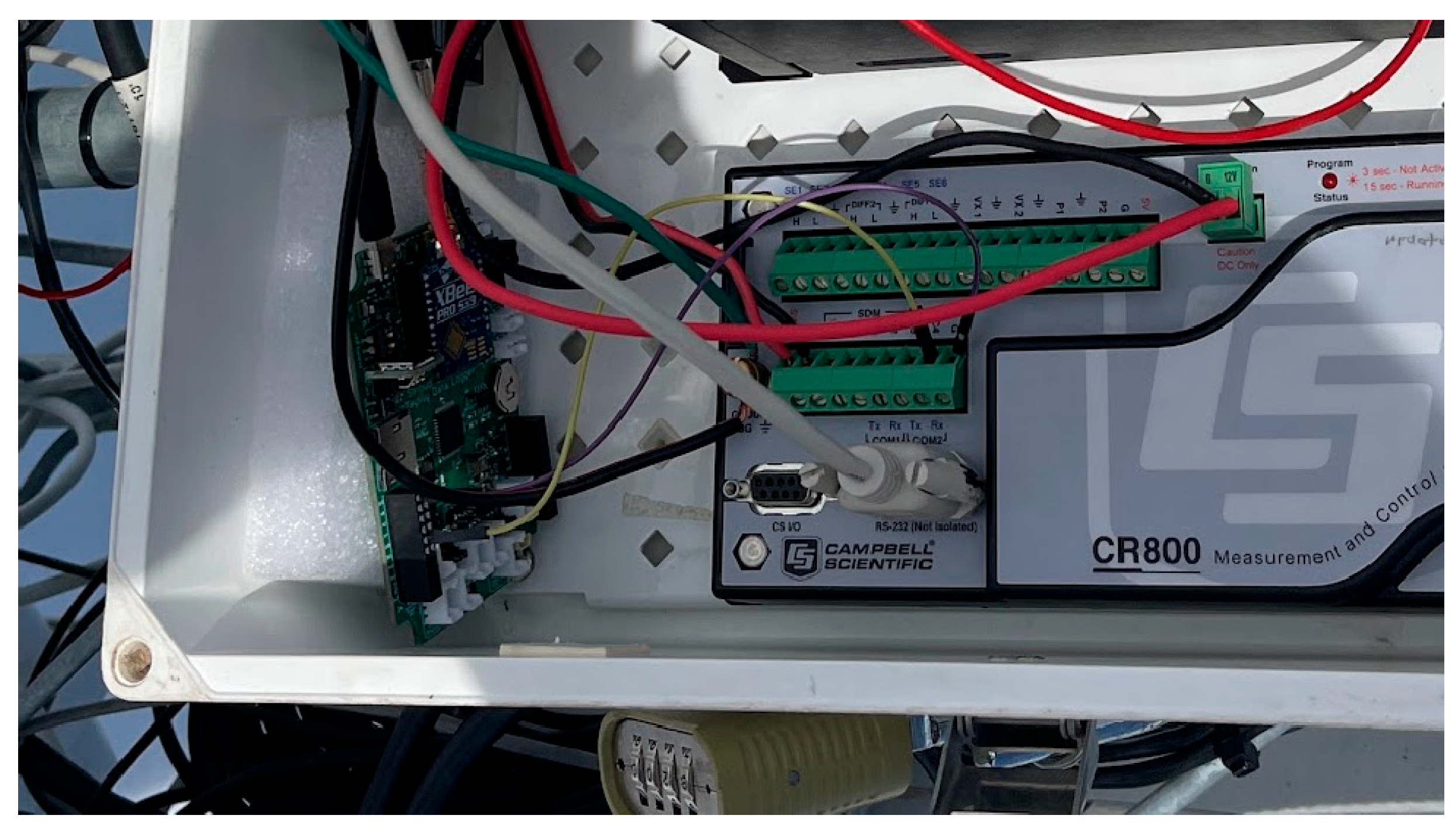
• If expanding on an existing monitoring network that uses dataloggers other than the Mayfly (e.g., a network of Campbell Scientific Dataloggers), the datalogger that will interface with the new network of Mayflies needs to have Universal Asynchronous Receive Transmit (UART) serial capabilities.

We first provide an overview of the data communication and networking system design, after which we describe each of the technical components of the system within the sub-sections that follow. For a network of snow sensing stations without a cellular Internet connection at their location, the concepts of “base” stations and “satellite” stations were adopted from common radio network architectures. In this study, we define a satellite station as a monitoring location with a Mayfly datalogger that collects data using the ModularSensors library. These stations have an RF Bee module that enables communication with any other station in the network, whether satellite or base. Base stations are those within a network that have Internet connectivity, whether through an existing telemetry network or through cellular data service and are responsible for the aggregation of data from all stations making measurements in the network.

Figure 3 shows the architecture of the base-satellite system and the flow of data from satellite stations to the Internet. Each datalogger in the system has one or more associated methods of communication with other dataloggers indicated. All data eventually goes to a HIS, which is an Internet server that stores and manages hydrologic data. Note that there can be more than one satellite station for a network.

The base station has a Mayfly datalogger that uses a 900 MHz spread spectrum Bee module to retrieve and aggregate observations from all satellite stations within a network. The base station Mayfly uses a jumper wire to communicate serially with a second Internet-connected datalogger housed in the same enclosure. The second datalogger can be a Mayfly with a cellular LTE Bee connecting it directly to the Internet, or it may be another datalogger with some other connection to the Internet (e.g., a Campbell Scientific datalogger connected to an existing Campbell telemetry network). A Mayfly datalogger can only have one XBee module connected to its header, which prevents a single Mayfly from serving as a base station—and thus the second, Internet-connected Mayfly uses a cellular LTE Bee. Where the Internet-connected datalogger is not a Mayfly, the only requirement is that it must be capable of serial communication with the base station Mayfly.

In the use-case where a snow sensing station makes measurements and has its own cellular Internet connection, the base station is omitted, and data is sent to a HIS server directly from the same datalogger that makes measurements. This architecture is shown in Figure 4.

2.5.1. 900 MHz Radio Module Selection

The 900 MHz radio modules selected for this system are Digi’s XBee Pro S3B 900 MHz module [43]. These Bee modules can transmit signals up to nine miles (approximately 14.5 km) and are capable of meshing with other XBee Pro S3Bs. Each module has a SubMiniature version A (SMA) coaxial antenna connector, making it compatible with many antennas such as an omnidirectional dipole whip antenna, or it can work with reverse-SMA (RSMA) antennas, such as the Yagi, with the help of a converter. The XBee Pro S3B also has a sleep mode that can be programmed to be pin driven.

The XBee radios are programmed using Digi International XCTU software (https://www.digi.com/products/embedded-systems/digi-xbee/digi-xbee-tools/xctu). The radio module can be customized to perform according to different use-cases, but for this application, the settings listed in Table 5 are changed from the default radio settings. These configurations facilitate mesh communication between radio modules with power to the radio modules being controlled by the Mayfly datalogger.

2.5.2. LTE Radio Module Selection

For networking scenarios where the Internet-connected datalogger at a base station is a Mayfly, or for directly connecting to the Internet from a singular station where measurements are being made with the ModularSensors library, we selected the EnviroDIY LTE Bee as the communication module [44]. This module was chosen because source code has already been developed within the ModularSensors library for publishing data directly from stations using Mayfly dataloggers using HTTP POST requests, and the class methods in this source code can be extended and used for publishing data to Internet servers outside of those already included in the implementation of ModularSensors.

2.5.3. Mesh Network Design

Snow sensing stations may need to be deployed in remote areas without cell coverage that may be covered by trees, foliage, or obscured by topography. Configuring the XBee Pro S3B with their mesh setting allows for wider coverage and more redundant communication because all satellite stations in a network can help facilitate message transmissions between any station and the base station. However, this means that if the stations are to save on power by only turning on radios when needed, all the radios need to be powered on at the same time during communication to establish the mesh network.

Due to the potential remoteness of some stations, a satellite station may not be useful in mesh networking once its own data is sent because it may only be able to talk to one other station (e.g., exterior or leaf nodes in the network). To save on power, we developed an approach of progressively retrieving data from the most remote or isolated satellite stations first, shutting down their radios to conserve power, and then moving on to the stations having more connections with other stations in the network (e.g., interior or repeater nodes in the network). This maximizes the number of potential mesh pathways messages can use while reducing power consumption at stations that do not need to relay signals.

A repeater station may be necessary within a network if a radio signal cannot be established between a satellite station and any other network station. Repeater stations are deployments that do not make measurements but add a Mayfly and XBee to a location that bridges a gap between the desired satellite station and another station within the mesh network. Repeaters may connect directly to the base station, or they may connect with one or more satellite stations in the mesh network.

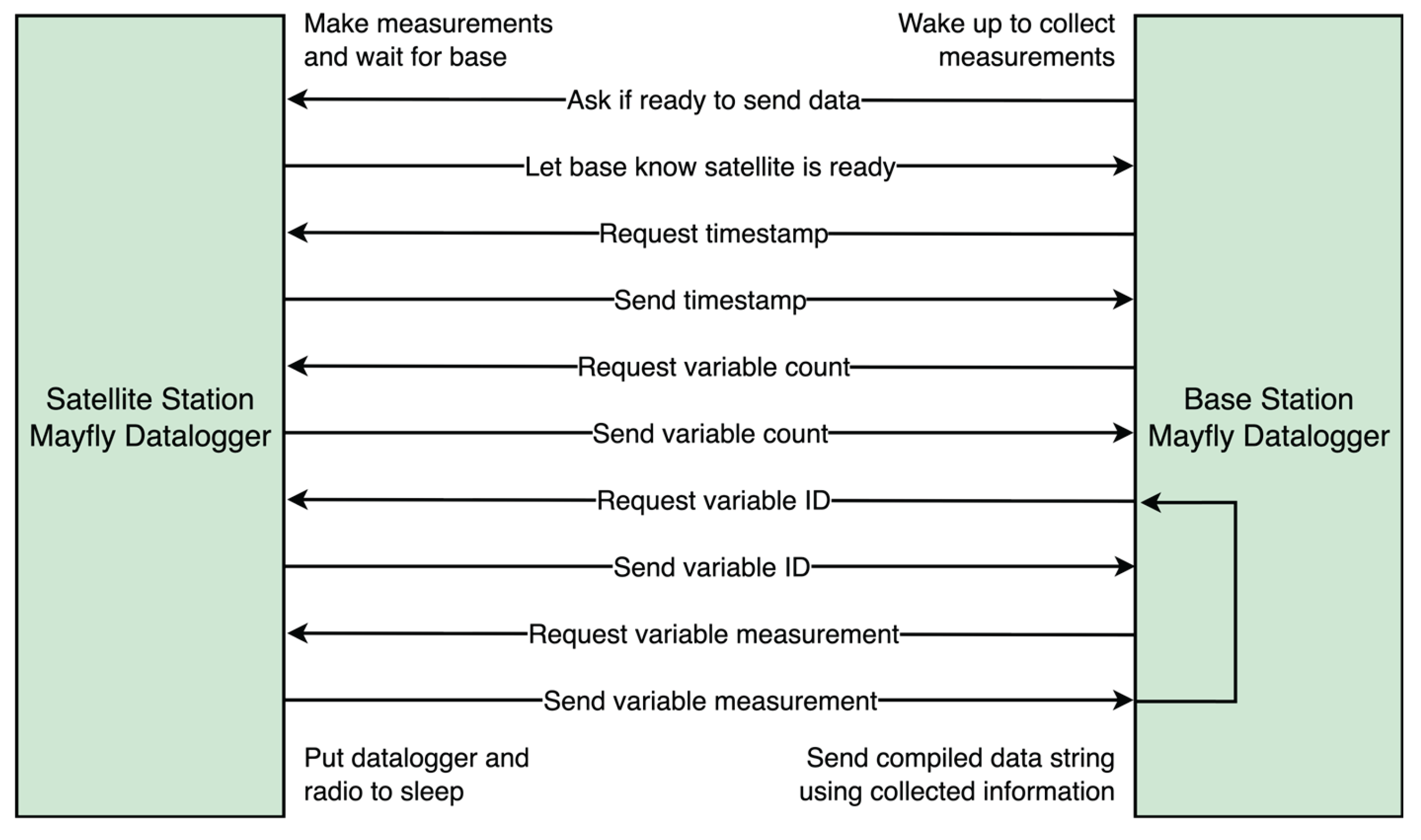
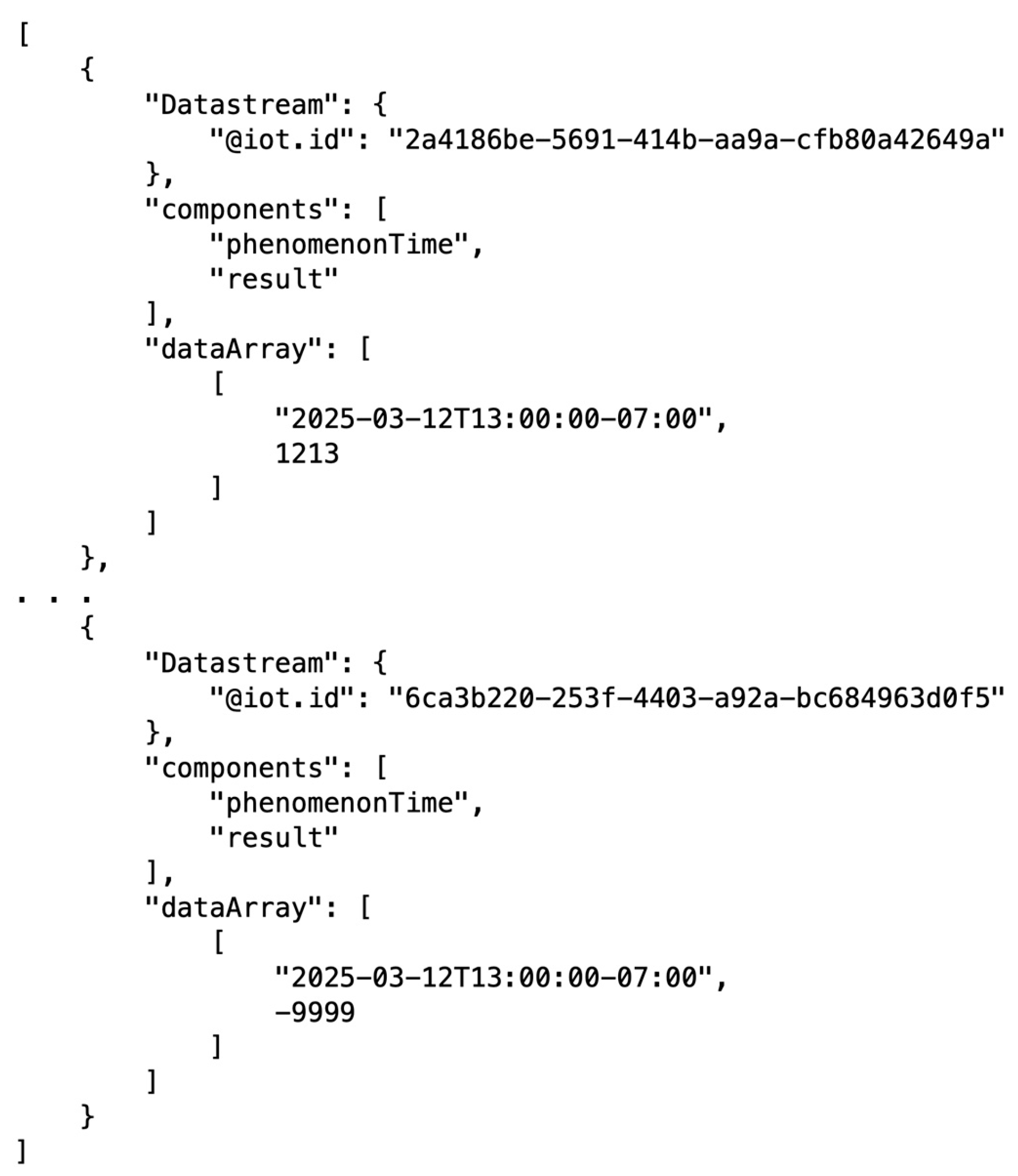
2.5.4. Communication Protocols

Because the XBee radios are generic communication modules that can transmit any message between two dataloggers and any message can be sent between two devices using a UART serial port, we had to design communication protocols to enable communications between satellite station Mayfly dataloggers and the base station Mayfly datalogger, which orchestrates communications within the network, over their XBee modules. The protocols we designed and implemented include determining when communications happen, the order in which messages are sent, handshaking communications between stations in the network, the content of the messages to be sent, and ensuring that messages are correctly sent. We also had to design communications between the base station datalogger and an Internet-connected datalogger co-located with the base station. First, the base station datalogger must pull data from satellite stations rather than having satellite stations push data. This ensures that two satellite stations do not try to communicate with the base station at the same time, helping reduce noise and keeping the communications buffer space open. This also allows for more leeway with communication time windows because a satellite station can wait for the base station to reach out to it rather than having all satellite stations try to send data to the base station at once.

Second, data from the base station datalogger must be pushed to the base station Internet-connected datalogger. Because there is only one line of communication occurring between these two dataloggers, pushing data into a sufficiently sized buffer on the Internet-connected datalogger is easier than establishing a pull-based data transfer. Communication between dataloggers must use asynchronous handshaking via a request/acknowledge protocol without relying on a shared clock or timing signal. Because the real-time clocks of dataloggers without direct cellular Internet connection are not synchronized, time-synchronized communication methods cannot be used. Additionally, fail-safe protocols must be present at all steps of pull communication in case communication is interrupted. This ensures that a satellite station datalogger does not get stuck in the communication parts of its program when errors occur and can return to normal data collection duties so that observations are not missed.

Depending on how an XBee Pro S3B is configured, it may expect outgoing messages to be formatted a certain way when they are received from its datalogger, and it may deliver received messages in a specific format that must be handled by the connected datalogger on the other end. This configuration refers to its data framing methods. There are two types of data framing used by XBee modules, transparent and API mode [45]. In transparent mode, whatever a datalogger sends to its connected XBee will be immediately sent as is to the receiving XBee it was configured to send data to. There is no quality assurance checking within the message. The receiving XBee transmits the bytes of received information (either to a downstream XBee module or to a connected datalogger) exactly as they arrived, even if they were corrupted.

API mode is a Digi method of sending data in what they term “frames.” Frames usually consist of starting characters, the type of frame, such as a received message or a restart message, information about where the message came from if relevant to the frame type, and a checksum which is a mathematical gut-check that all the bytes came through uncorrupted. For our network design, we chose to send and receive all messages between stations in API mode because of the greater quality assurance that can be achieved using frames and because API mode allows code running on the datalogger to determine optimum network paths (the datalogger’s code determines where messages will go) rather than requiring radio modules to be hard programmed with set network paths. In transparent mode, the destination radio must be programmed into the XBee’s settings before adding the XBee to the datalogger, so it must be removed and reprogrammed if it needs to send messages to a new datalogger. It is also easier to troubleshoot and debug in API mode because the XBee will send back error frames if a connection was not established, which is not the case for transparent mode.

To send a message using the XBee module, a transmit request frame type needs to be constructed and pushed from the datalogger to the attached sending XBee. This frame type requires that the datalogger provides the serial address of the receiving XBee, length of the message, the body of the message, and a correct checksum. The XBee gets this frame of data from the datalogger and checks it itself. If anything is wrong, it will not send the message. The receiving XBee will get a message from the sending XBee and produces a receive packet frame, where it tells its datalogger who the message came from and what the actual message is. Communications cannot occur without these structures. The Mayfly datalogger code developed for this system handles the construction of these frames, which are the actual messages and handshaking that make up the protocol of their communication.

Every Mayfly datalogger has a real-time clock that helps ensure the regularly scheduled measurement and local logging of data to an SD card. We programmed all of the satellite stations and the base station Mayfly datalogger to turn on their XBees immediately after recording sensor measurements to the SD card. The measurements are recorded on the hour. The base station Mayfly turns its XBee module on at the logging interval and begins requesting data in a station sequence programmed into it according to the mesh network design in Section 2.5.3. Because the communication is asynchronous, each satellite station Mayfly must start in a listening state where it waits for a message addressed to its XBee module’s serial address. Because the XBee modules are programmed in a mesh configuration, the waiting satellite stations or repeater XBees will just help push messages along that are not addressed to them. Each satellite station acts as a repeater during the time the base station attempts to collect data from every other satellite station.

When a message arrives that is addressed to the satellite station, a series of exchanges take place between the satellite station and the base station. At any point in the handshaking, if a request cannot be fulfilled within a programmed timeframe, the satellite station will back out of its communications procedure, put its radio to sleep, and continue collecting data within its loop function. The base station will take what information it has and send it along to the Internet-connected base station datalogger, even if more variables could have been collected. Incomplete data points are not communicated. During the handshake process, the first exchange includes the base station requesting a ready signal from the satellite station. It does this by sending an “R” to the station. If the satellite station hears this signal, it sends back an “R” to the base station. The base station then begins constructing a string of characters that will be pushed to the base station’s Internet-connected datalogger. The first part of the string it constructs is the name of the station it is collecting data from. The format of this string is described below.

After this, the base station Mayfly requests the timestamp of the variables measured by sending a “T” to the satellite station. The satellite Mayfly retrieves the timestamp for the most recent measurements from its memory then reports it back to the base station. The base station Mayfly adds the timestamp to its string of data then requests the number of variables the satellite station measured. The satellite station retrieves this number from its memory and reports it to the base station Mayfly. This number is not used as a reported data point but rather helps both the satellite Mayfly and the base station Mayfly know how many times the base station Mayfly will loop asking for each variable name and associated measurement.

After receiving the variable count, the base station Mayfly begins asking for each of the variables measured within a code loop. These are each of the variables listed in the satellite Mayfly’s variable list developed in the ModularSensors code. The base station Mayfly asks for the name of the variable using the code loop’s current index. The satellite station pulls that name from the variable list it has created in memory and reports it.

The base station Mayfly records that to the data string and then asks for the observed data value of that same index. The satellite station retrieves that value and reports it. The base station Mayfly then records the value and moves on, repeating this in a loop until the number of variables is reached. Once all variables are reported, the satellite station puts its radio to sleep because it no longer has data to report. If station sequencing was done correctly, the satellite station that just reported its data to the base station will no longer meaningfully contribute to mesh networking. The entire communication process (Figure 5) is incorporated into the loop function of the Arduino sketch running on the Mayfly dataloggers.

The final message of data sent to the Internet-connected datalogger from the base station Mayfly needs to have a clear structure that can be parsed by a generic string parser in the datalogger’s programming language—whether it is a Mayfly datalogger or some other datalogger such as a Campbell Scientific datalogger. This enables the extraction of data from strings of characters sent between the two dataloggers. The following structure was created to format messages sent between the base station’s dataloggers:

@variableIdentifier=variableMeasurement;

The “@” character denotes the start of an observation data point, with the ASCII characters between it and the equals sign (denoted as “variableIdentifier” above) being an identifier that the Internet-connected datalogger will need to post the data, such as a Universally Unique Identifier (UUID) or a variable name. The programming of the Internet-connected datalogger will vary depending on how data is being stored and published in the already existing network, and not every use case can be explored here. However, Section 3.1 explores what this looks like for two important scenarios: 1) when the Internet-connected datalogger is a Campbell Scientific datalogger, and 2) when the Internet-connected datalogger is a Mayfly datalogger with an LTE Bee.

The characters after the equals sign (denoted as “variableMeasurement” above) encode the numeric value of the observation, also in ASCII characters, terminated by a semicolon. Strings of this format are used to differentiate between the various observed variables and their corresponding measurements made at a station. An example of a string of variables might be:

@station=marshes;@timestamp=2025-01-09 14:00:00;@snowDepth=653;

In this example, the satellite station data being sent from the base station Mayfly to the base station Internet-connected datalogger is the “marshes” station, with a timestamp of January 9, 2025, at 2:00 PM, with a snow depth of 653 millimeters. Any number of variables/observation values can be added to this string of data.

Because the communications between the two dataloggers at the base station are asynchronous, the Internet-connected datalogger also needs a way to determine when there is no more data for a satellite station in the string. To accomplish this, the base station datalogger adds a flag to the end of the string when all variables have been sent. Without the end of string flag, the Internet-connected datalogger might mistake data between stations. The end of station flag is a Boolean true for a variable “endofstation.” When it sees this, the Internet-connected datalogger assumes that the satellite station mentioned last in the string has no more data to be added for this timestamp. Below is an example of what this would look like in the string being transferred:

@station=marshes;@snowDepth=653;@endofstation=1;

When the Internet-connected datalogger receives this string from the base station Mayfly, it reads that the data coming in is for the marshes station. It then parses all the following variables until it reads that endofstation is true or has a value of one. After receiving the end of station flag, it will no longer parse data, and it will reset endofstation to false for the next string of data.

2.6. Deployment Platform

Two platforms were tested for deploying and mounting the necessary hardware for the snow sensing stations. One deployment platform uses a commercial-grade Campbell Scientific instrumentation tripod and grounding kit. This option was considered because many researchers may already have this equipment available on hand from other environmental monitoring projects. These tripods provide a durable and sturdy mounting structure and come in a package with many peripherals such as grounding rods, grounding cables, stakes, and guy wires. Figure 6 shows an example of this tripod in use. While robust, these tripods pose a significant increase in the overall cost of a snow station, with the tripod and grounding kit costing over $900 with an additional $400 for a guy wire kit. These tripods are also heavy, which makes them difficult to install in remote areas and on steep terrains, especially if deployment locations are only accessible on foot.

To address these limitations, we developed a second deployment platform (Figure 7) consisting of hardware pieced together from local home improvement stores and some online purchases. This platform consists of a single, vertical mast with a sensor crossarm that is secured at the base with a U-post and uses a guy wire kit for stability. It is relatively simple, lighter, and less expensive. Due to its off-the-shelf nature, however, it requires more time to gather materials since they do not all come from one place, but the deployment platform itself is about $1,100 less than the Campbell Scientific tripod kit.

Table 6 shows a cost breakdown of the deployment platform components for a snow sensing station using Campbell Scientific tripod kits. Table 7 shows the cost of off-the-shelf components sourced from either local or online retailers. Both platforms require similar waterproof instrumentation enclosures, sensor crossarm, and sensor mounts. While the component lists in the GitHub repository provide a less expensive instrumentation enclosure option, we found that they were not reliably water-tight. Thus, we recommend using the Pelican case listed here as the cost savings is not worth the risk of leakage. In the tables below we have specified a single instrumentation enclosure, but for applications requiring larger batteries a second enclosure may be needed. We also specified an inexpensive radiation shield for the air temperature sensor that worked well for our application and was significantly less expensive than the model sold by the sensor manufacturer.

3. Results

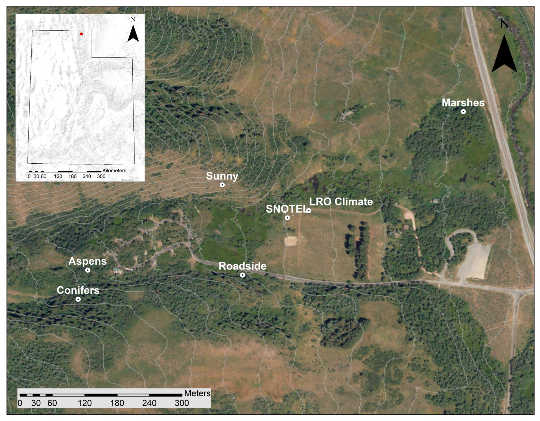
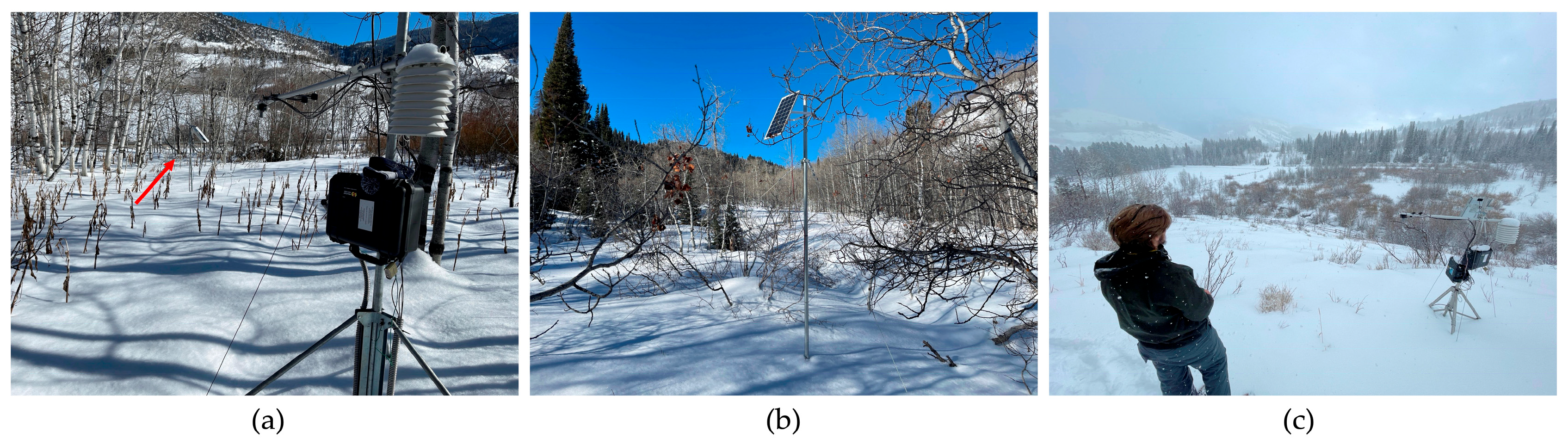
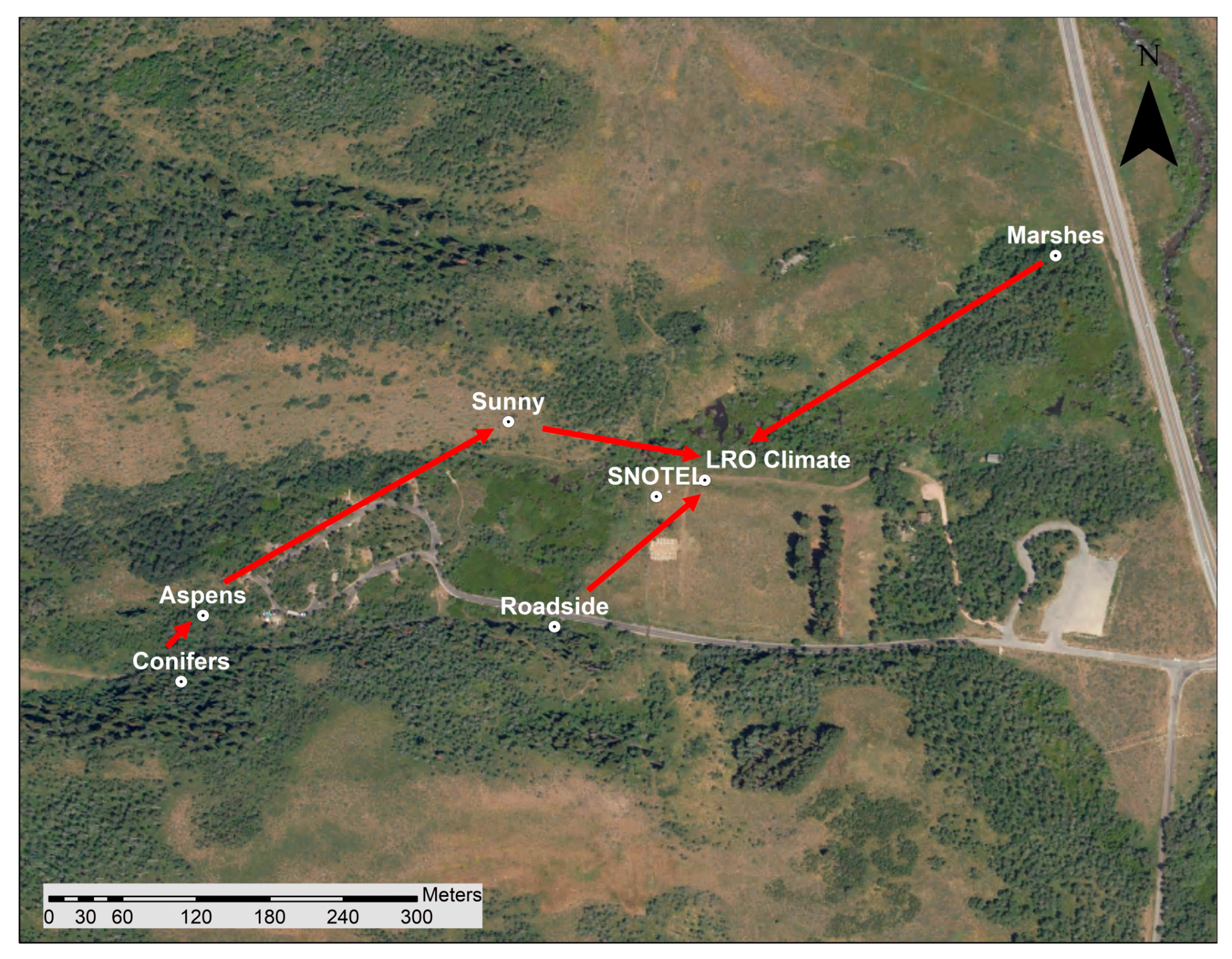
3.1. Case Study Implementations

The performance of the snow sensing station design and deployment was tested by constructing and operating five stations with different vegetation, aspect, slope, and terrain constraints in the Tony Grove Creek subbasin of the Logan River watershed near the TGRS and SNOTEL site. This area was chosen for its diversity of physiographic characteristics, including forested areas with both coniferous and deciduous canopies, variation in slope and aspects, presence or lack of exposure to the sun, and variable soil conditions with marshy riparian soils and more arid upland soils. This area also develops a snowpack each winter and is easily accessible during the winter given its proximity to a major highway. For more accessible testing purposes, a sixth station was constructed at the Utah Water Research Laboratory (UWRL) for testing sensors, deployment platforms, and communication protocols with the availability of a direct cellular data Internet connection.

The TGRS location is remote, providing the opportunity to demonstrate the use of 900 MHz spread spectrum XBee modules to create a local radio network that was then integrated with an existing Campbell Scientific radio telemetry and monitoring network that supports the Logan River Observatory (LRO) (http://lro.usu.edu). The UWRL station was deployed with a cellular LTE Bee module to demonstrate how singular data collection stations with a cellular data connection can send data directly to a HIS. Our goal in choosing these case studies was to demonstrate the variety of monitoring locations and network topologies that can be created using our station and networking protocol designs.

The five TGRS sites were deployed during the months of the winter 2024-2025 season and were named and characterized as follows, with Figure 8 showing their relative position to each other and relative to a co-located SNOTEL station and LRO climate station. Station locations were selected to represent a variety of physiographic conditions to enable study of the variability in processes controlling snow accumulation and melt. Thus, their locations were subject to different vegetation, aspect, slope, and terrain constraints. The LRO climate station was considered the base station, and an extra datalogger enclosure was added to the LRO climate station’s instrumentation tower so we would not disturb their operating instrumentation.

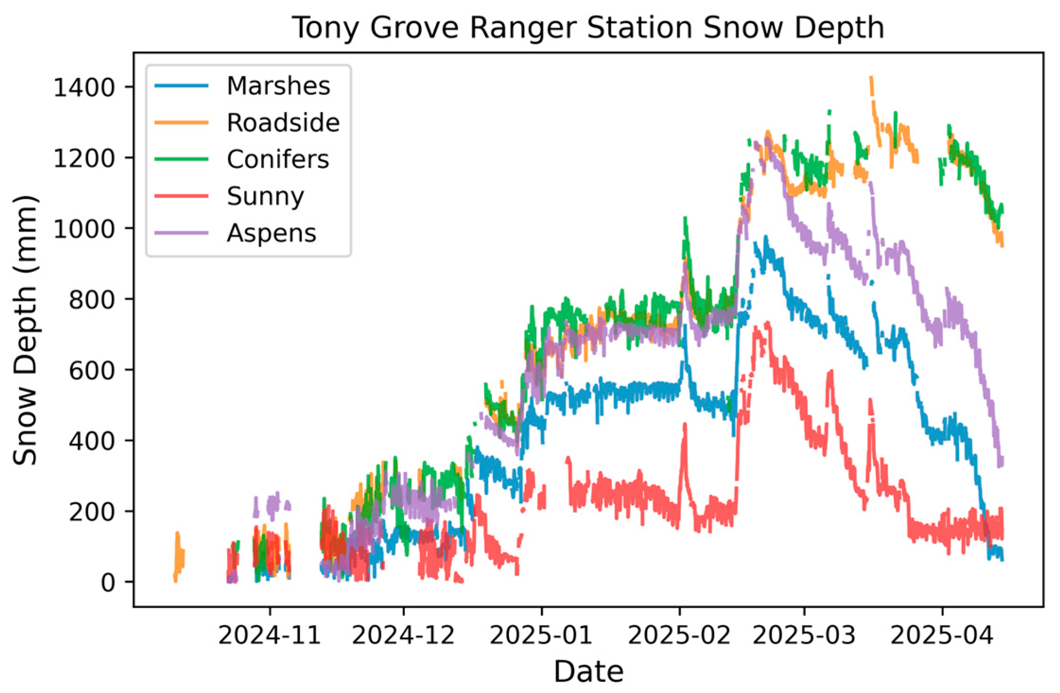
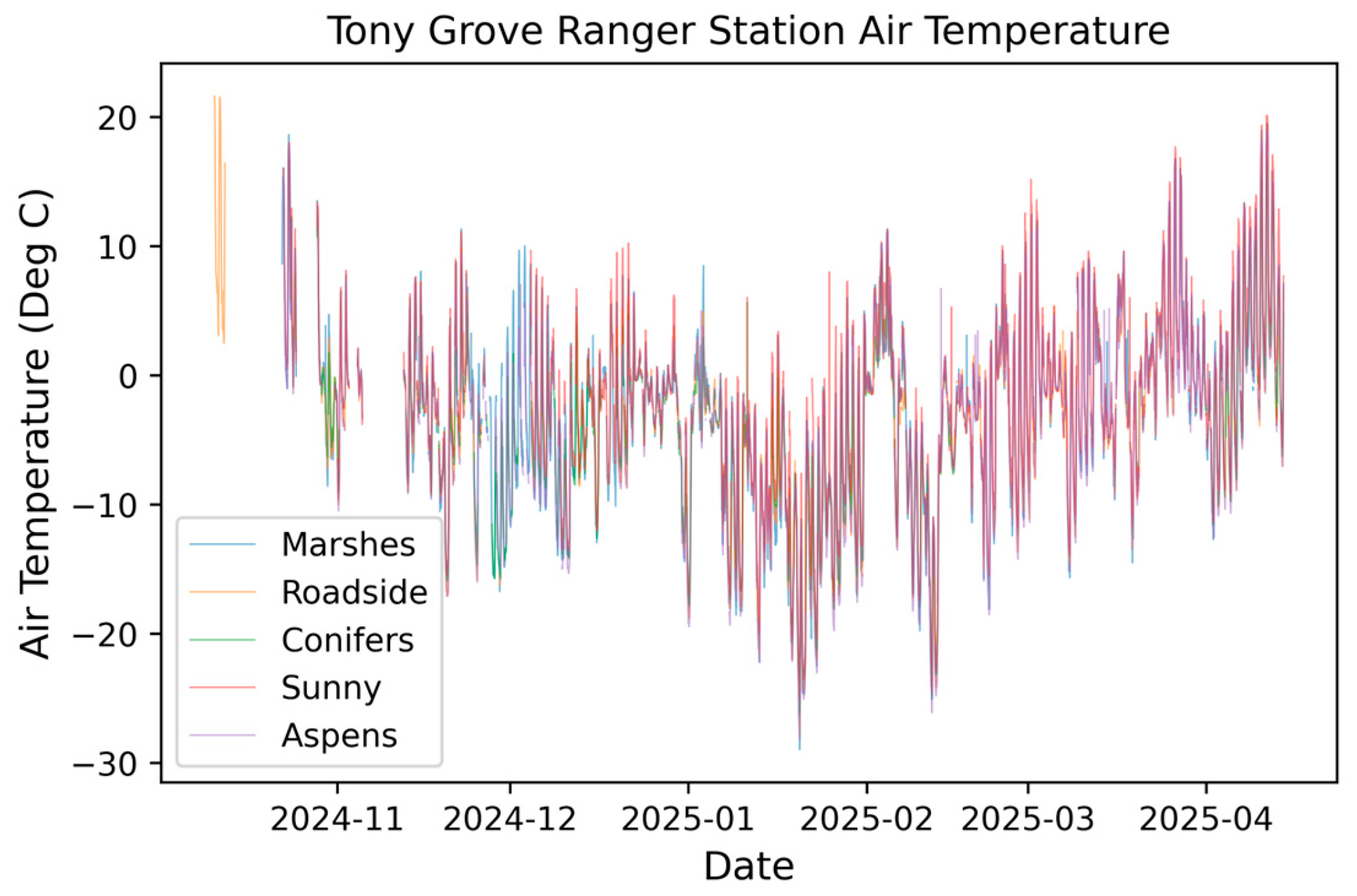
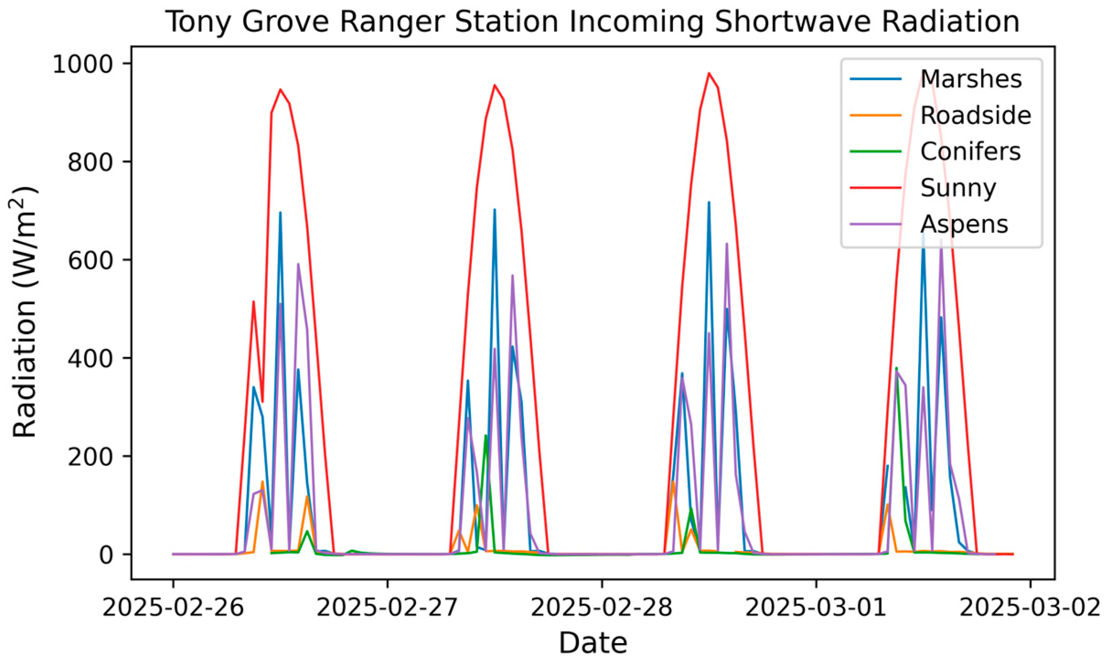
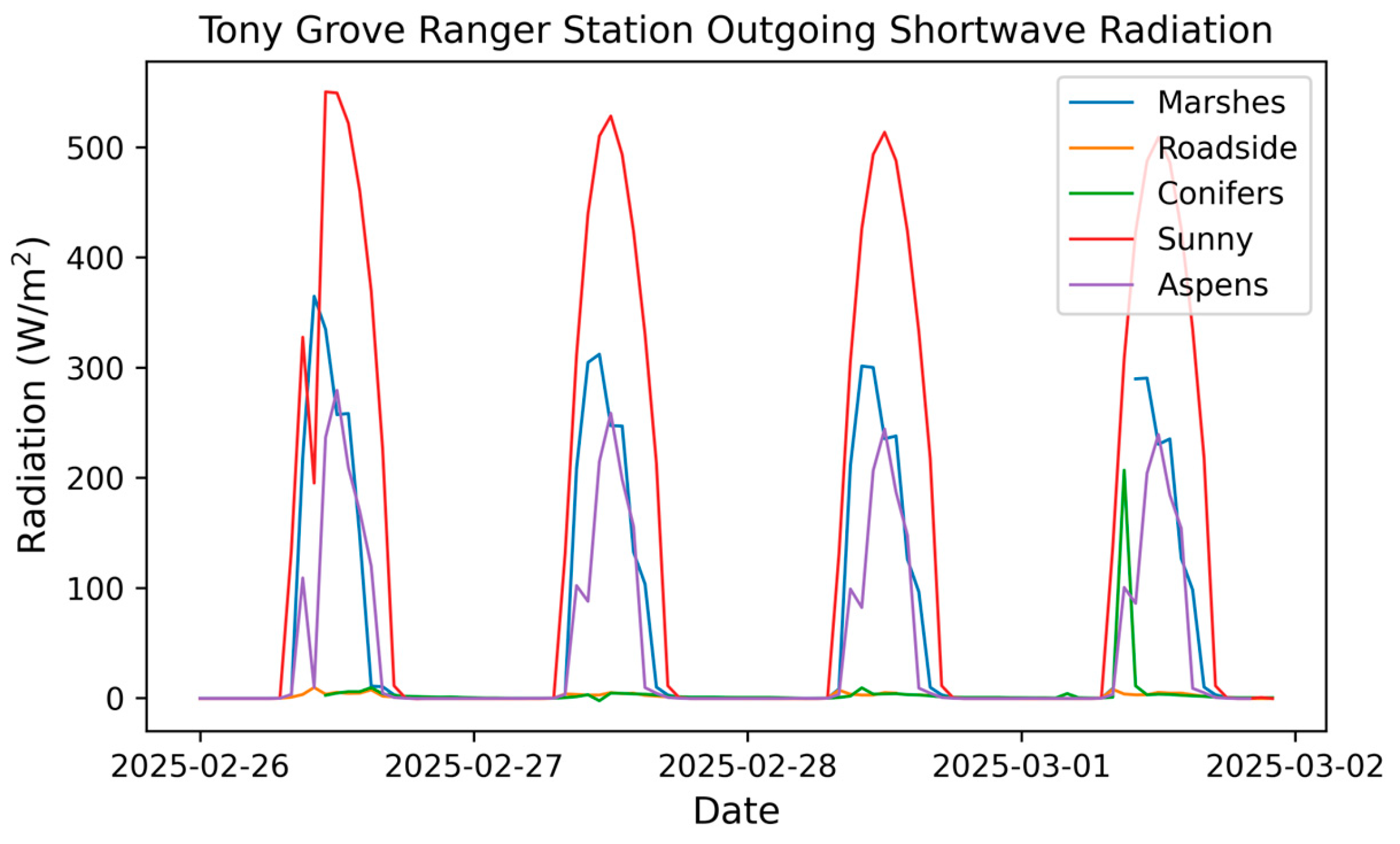
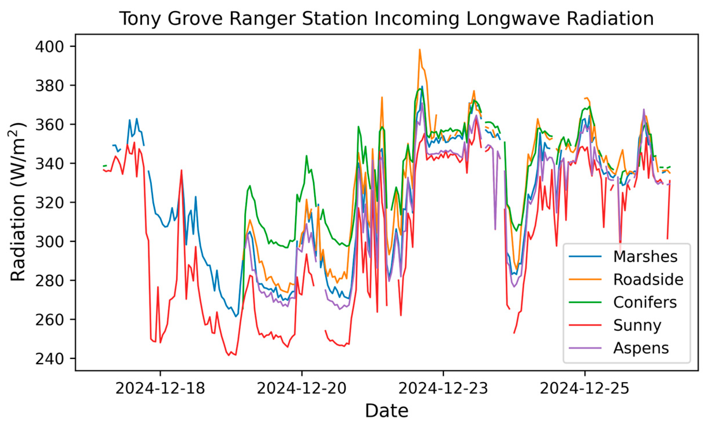
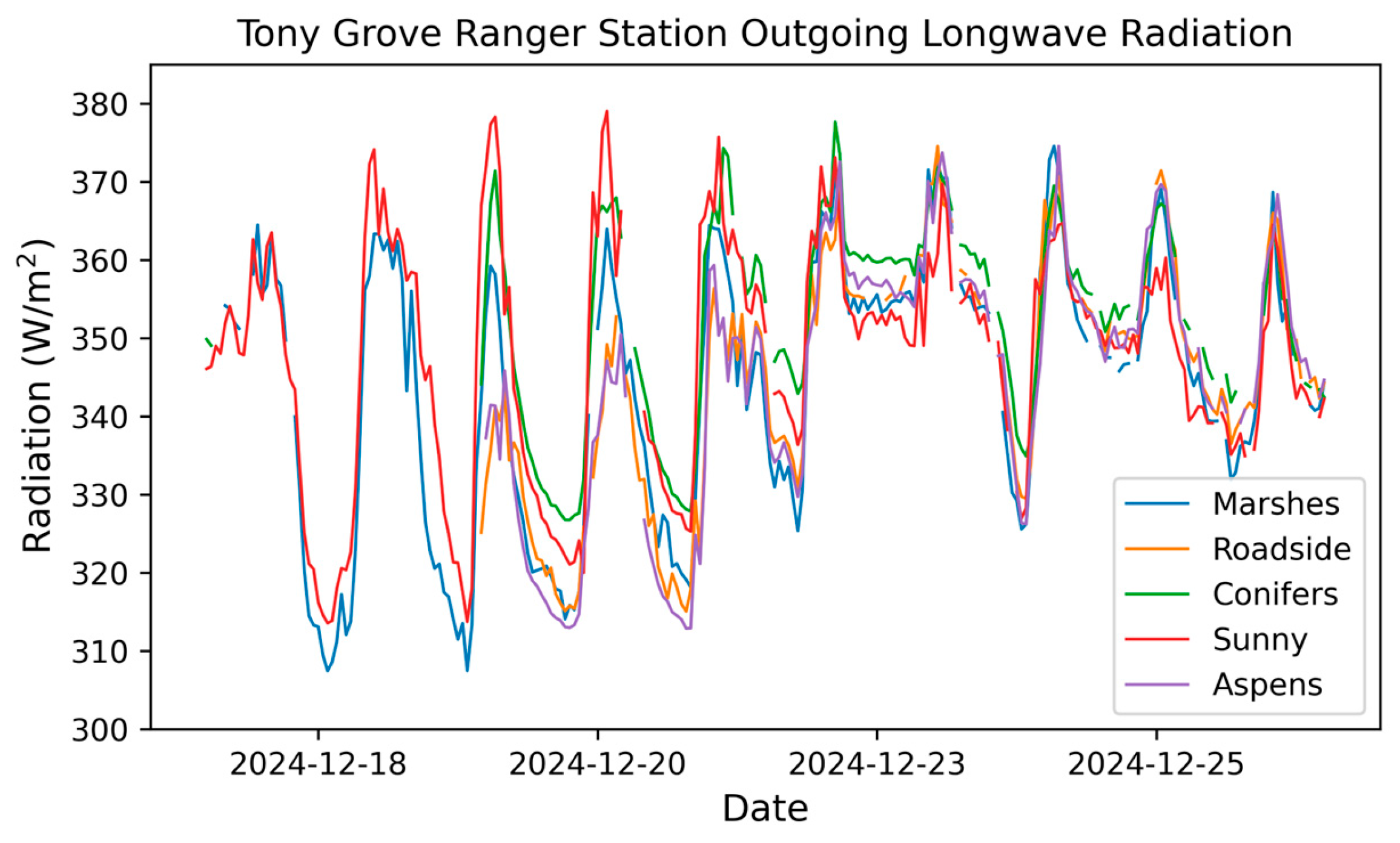
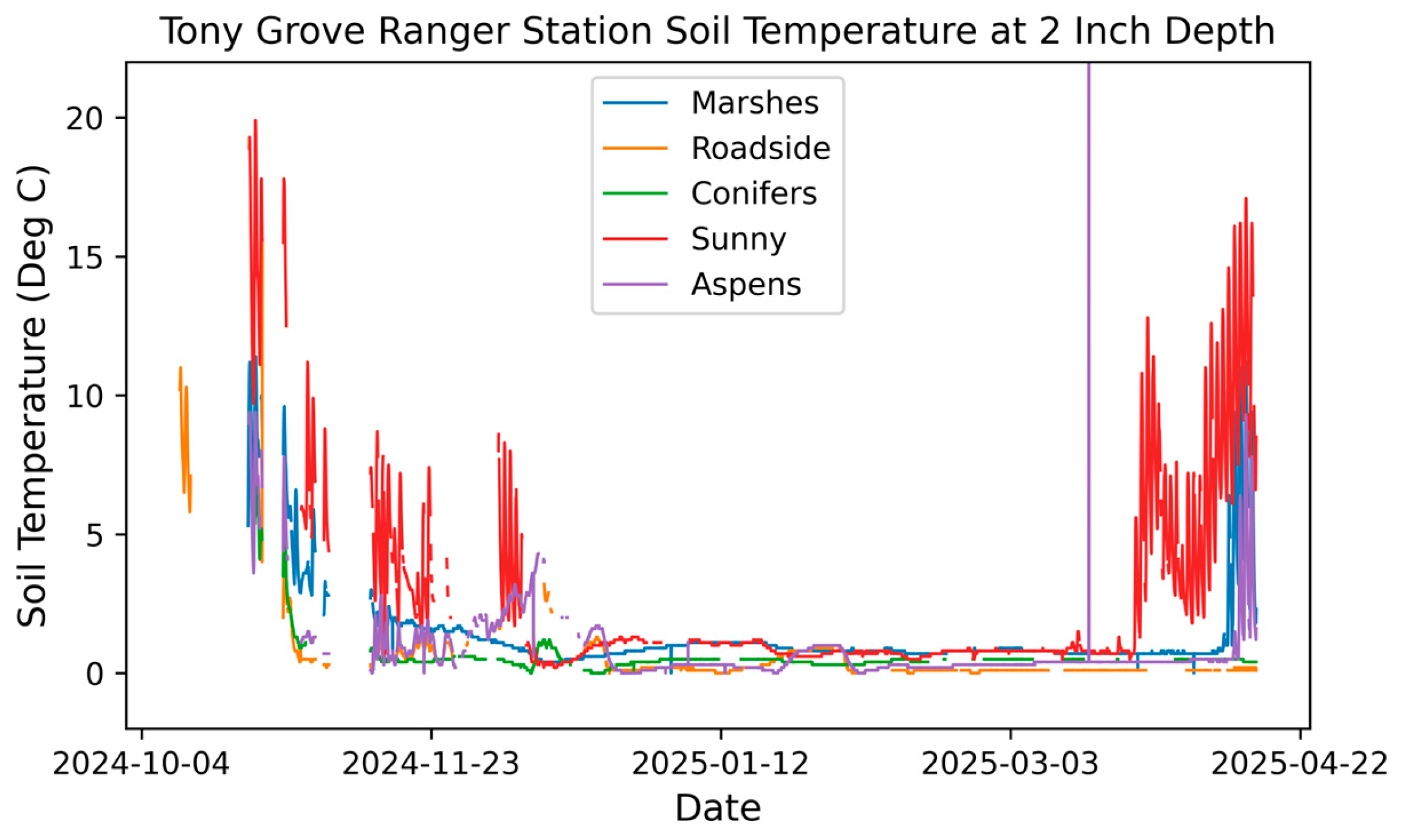
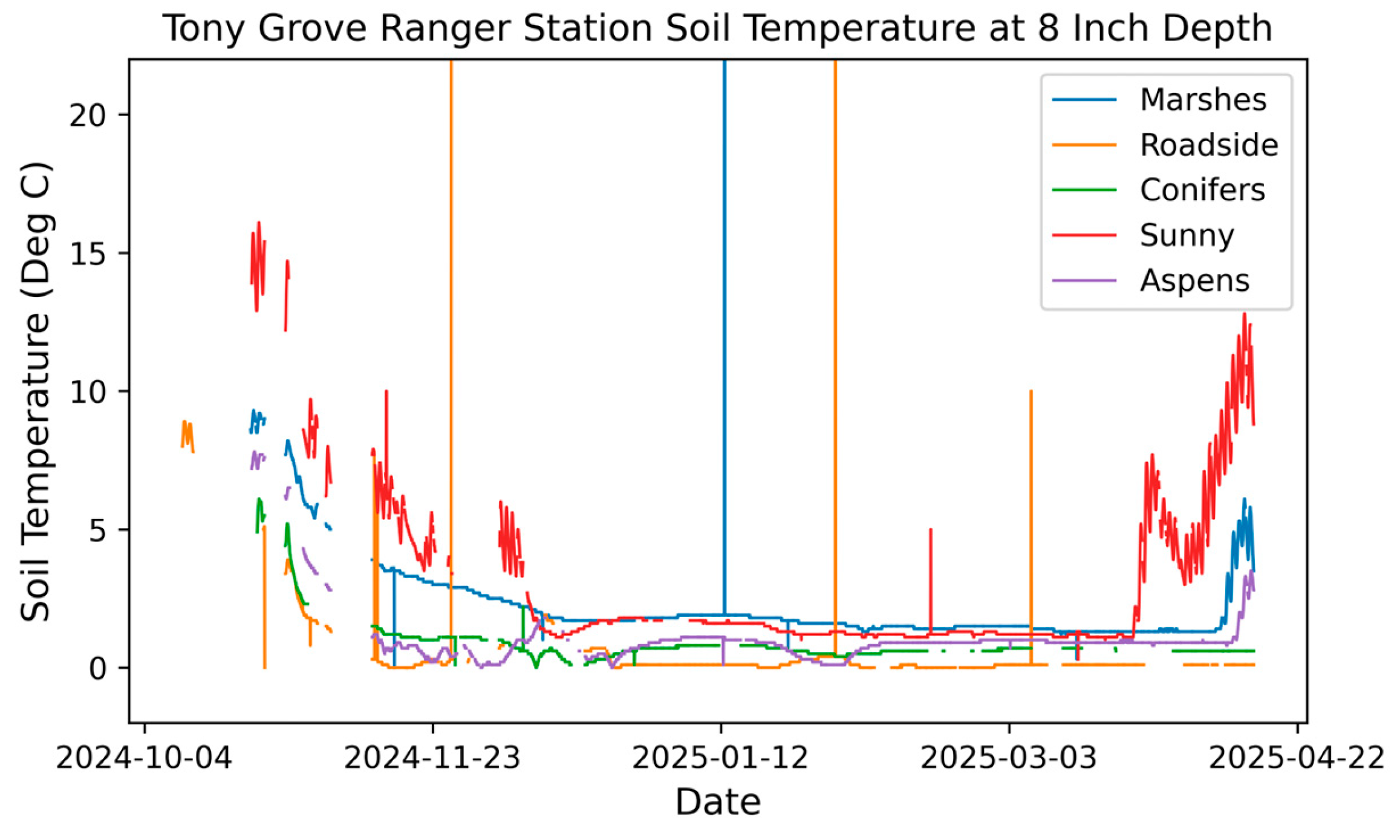
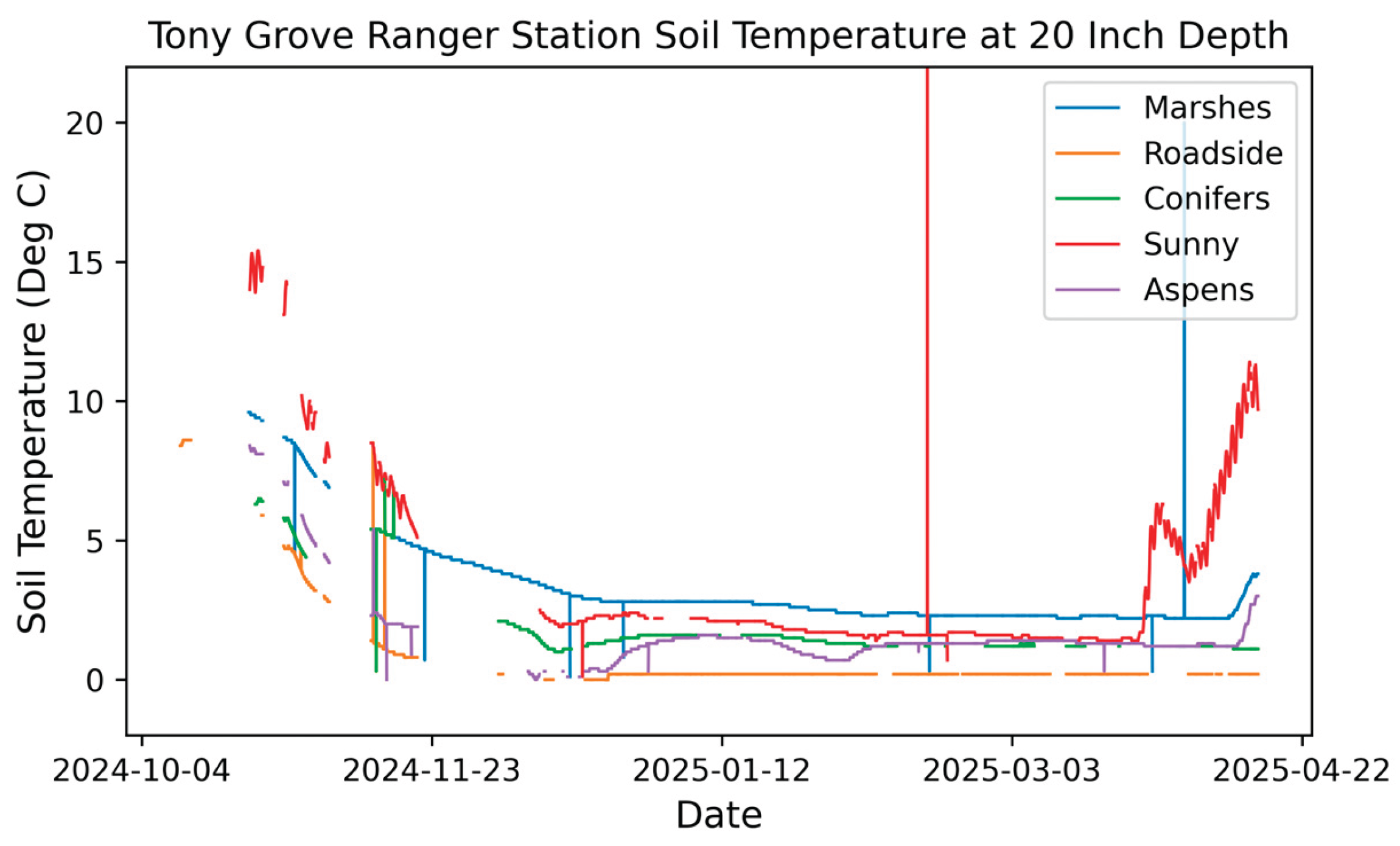
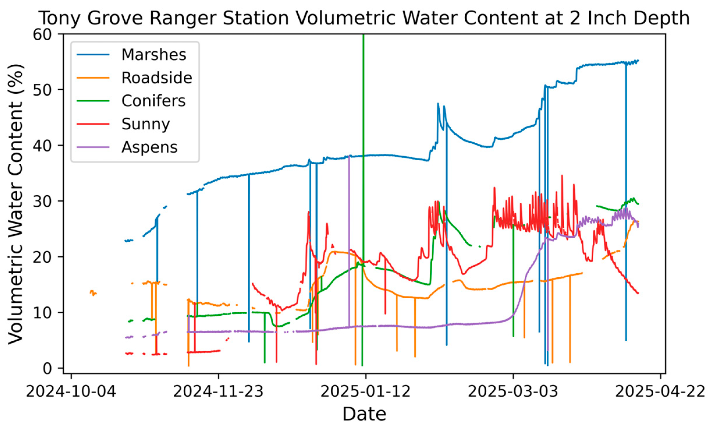
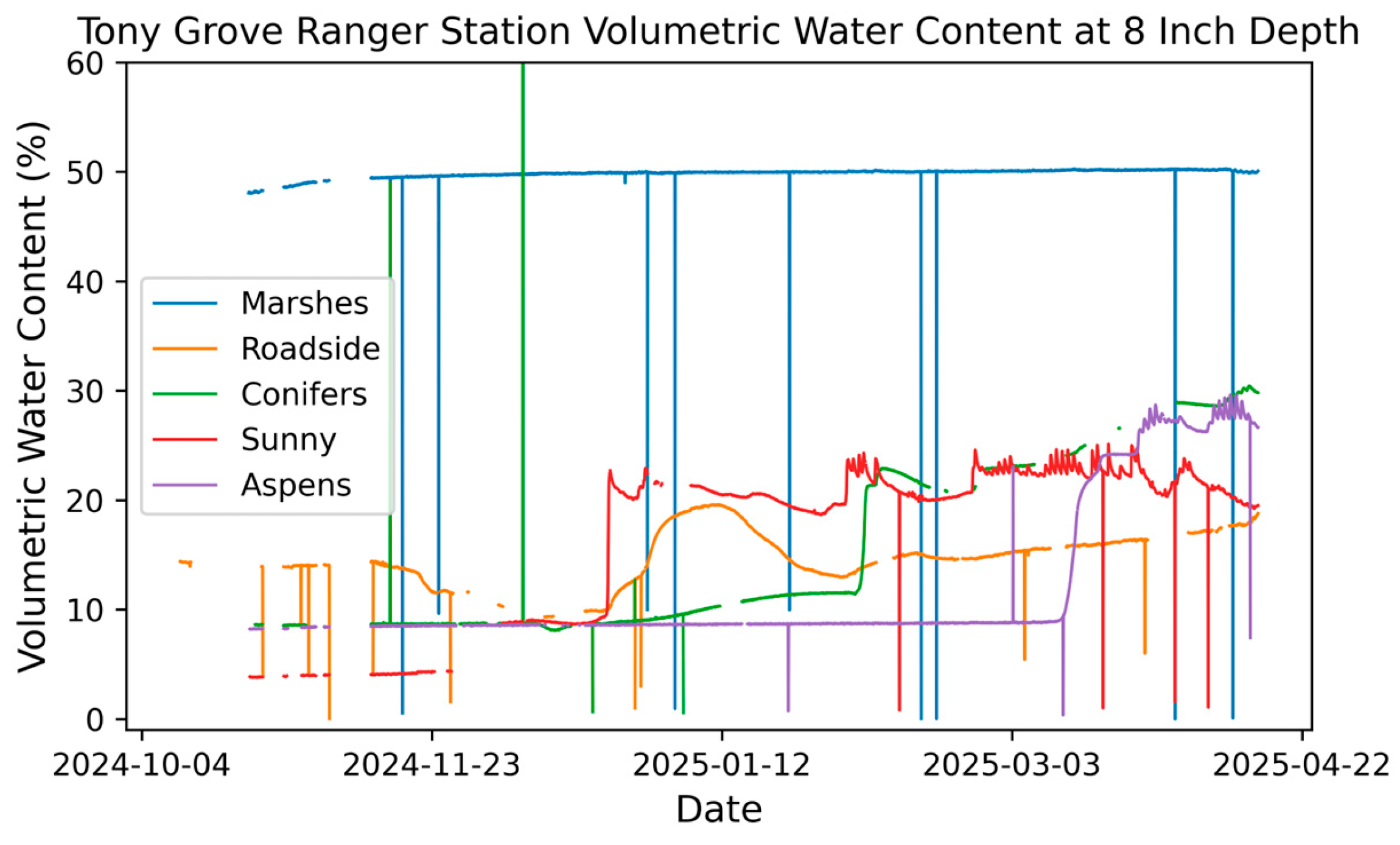
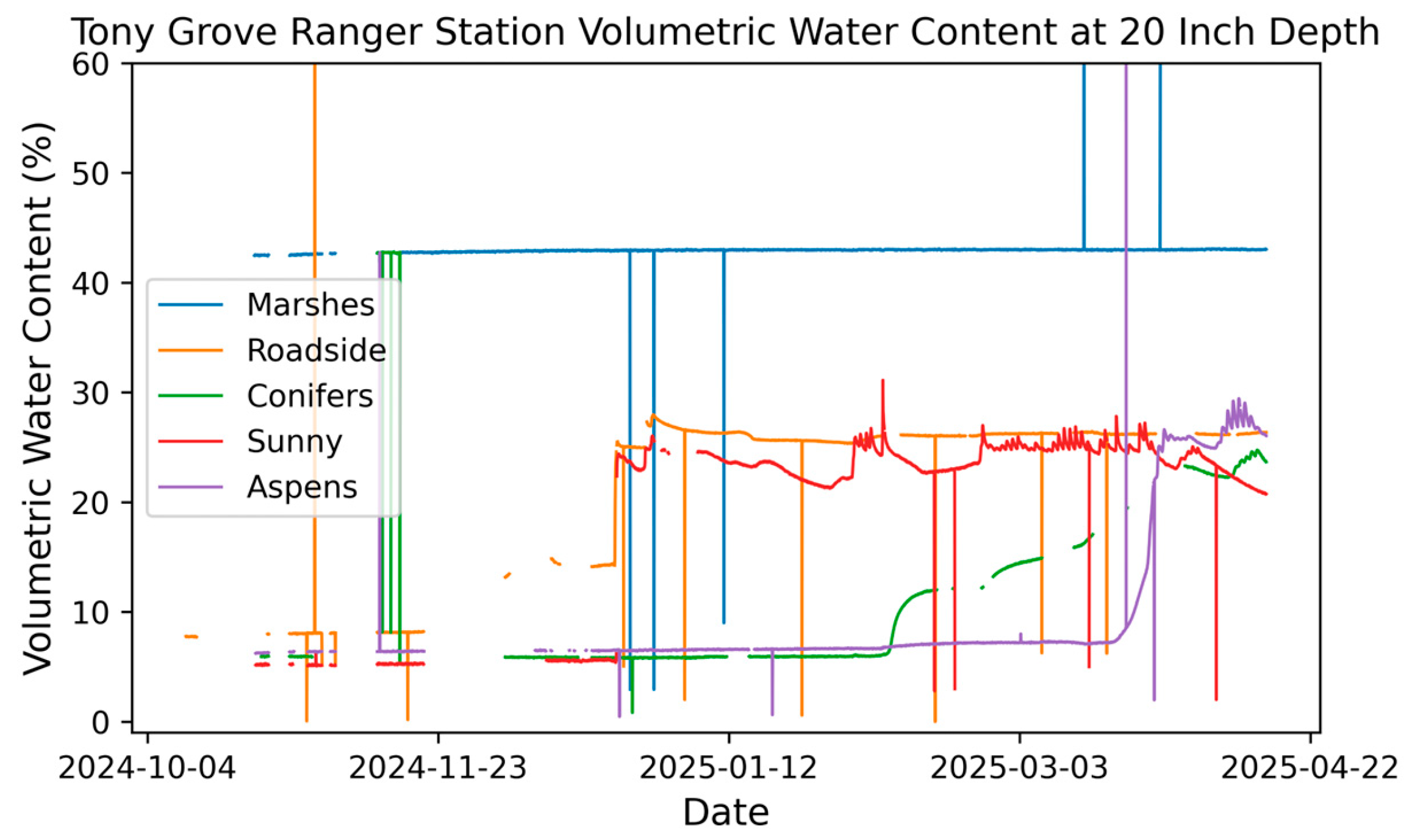
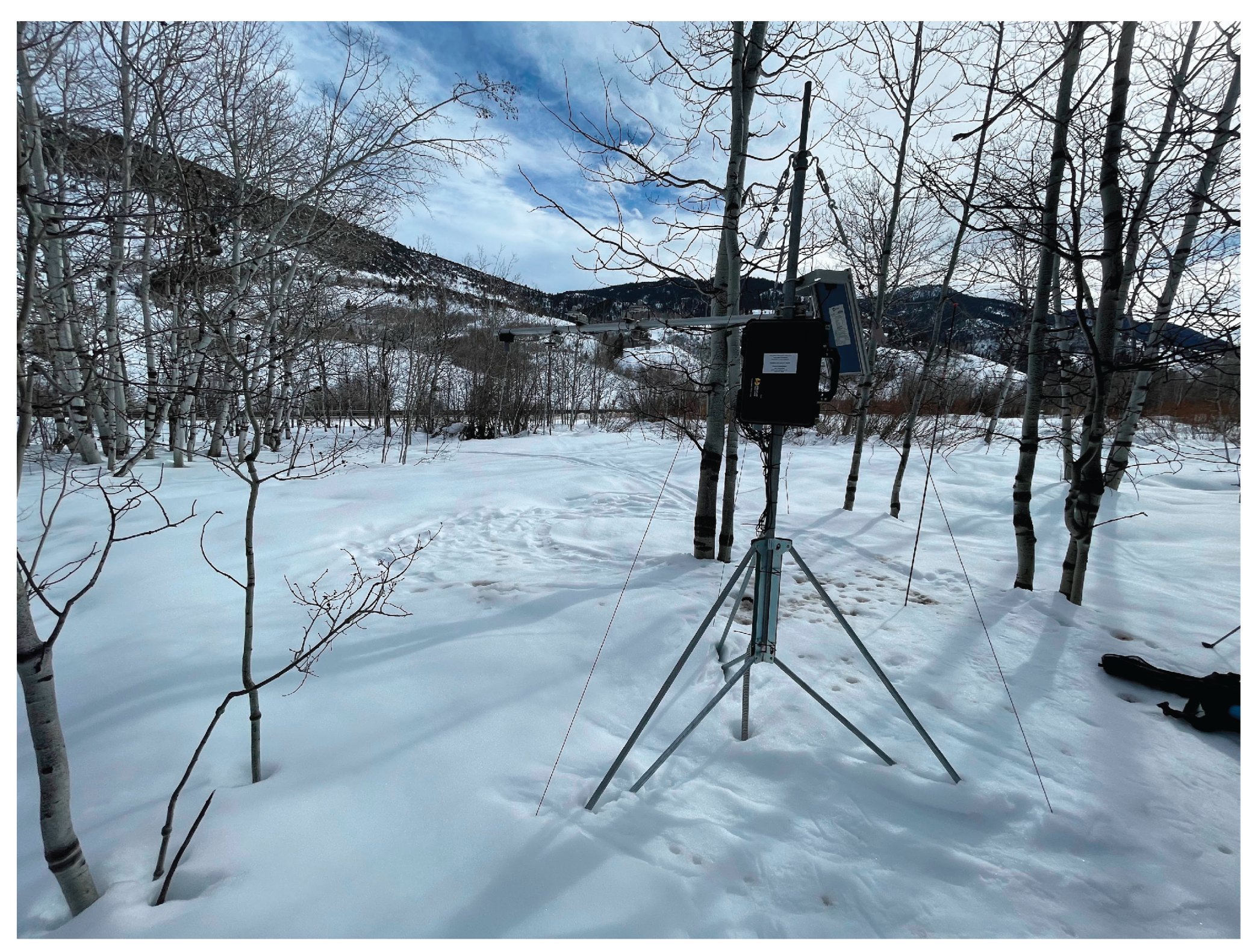
• Roadside: This site was chosen for its mix of coniferous and deciduous trees within the vicinity as well as its north facing aspect and lack of sun exposure.
• Aspens: This site was chosen for its heavy aspen representation, generally east facing aspect, and for having partial day sun exposure.
• Conifers: This site was chosen for its heavy conifer canopy, north facing aspect, and no sun exposure.
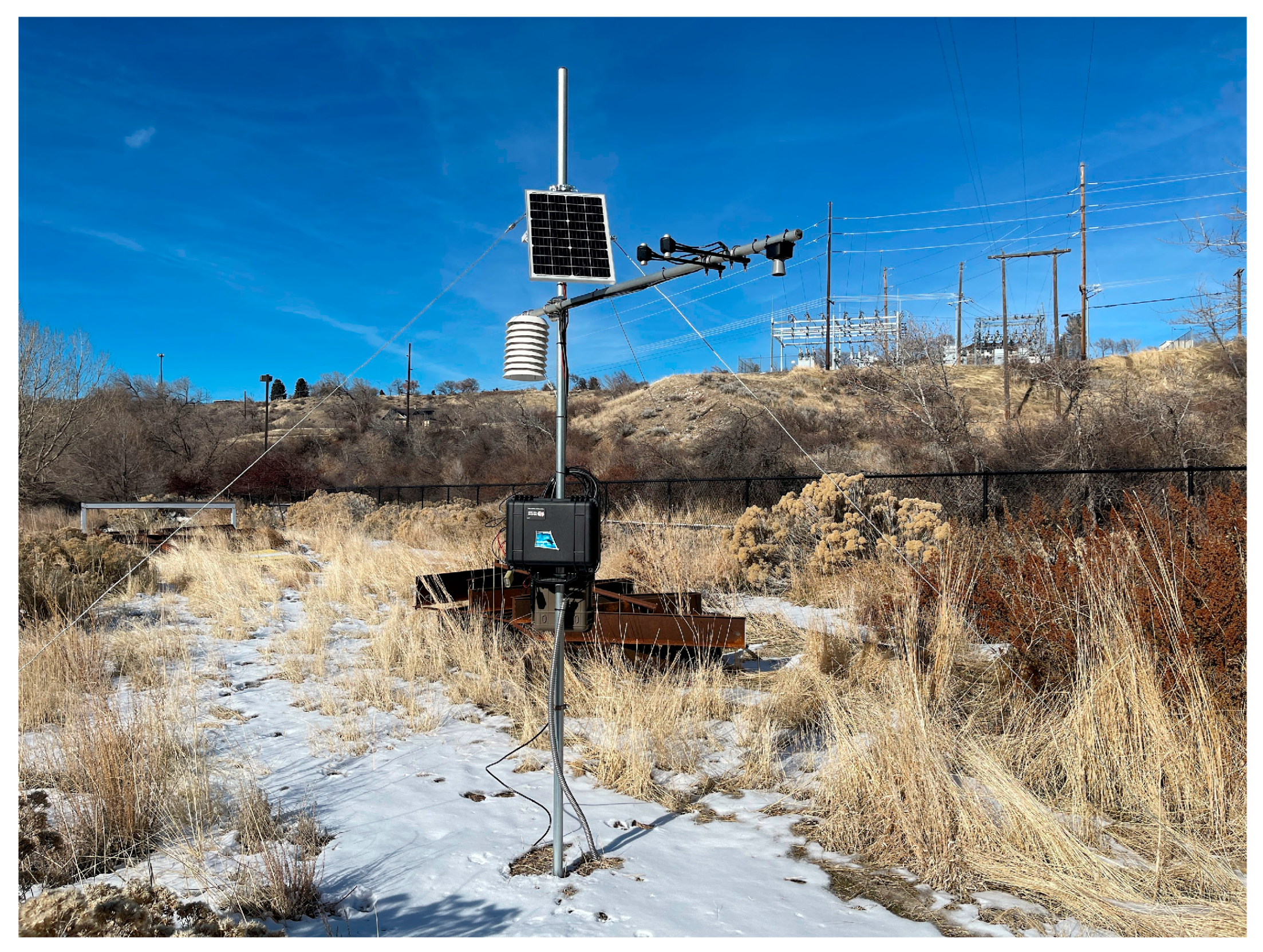
• Sunny: This site was chosen for its south-facing aspect, lack of tree canopy, full sun exposure, and dry soils.
• Marshes: This site was chosen for its general flat aspect, consistently wet soil, and aspen tree canopy.

We used Campbell Scientific tripods to deploy the five stations at the TGRS study area because we already had them. These tripods presented some difficulty in installation and takedown because of their weight, especially because some of our stations required a short hike to access. The UWRL station used the off-the-shelf version of a mounting platform. It was simple to construct and weighed less.

3.1.1. Station Power Considerations

Power was the most important consideration in customizing the design for each station. Each site varies in how much sun it receives, which impacted the appropriate battery sizes, solar panel ratings, and even solar panel placements. The Roadside and Conifers sites receive virtually no sun in the winter due to shading from topography and vegetation, making solar recharge impractical. The Aspens and Marshes sites receive partial to almost full sun depending on the location of the solar panel, and the Sunny site receives full sun. The logging interval for each station was set to 1 hour to match the logging interval of the SNOTEL station in the area.

3.1.2. Solar Panel Selection

Current draw measurements were taken at the Sunny station and assumed to be the same at all other stations because each has the same sensor and communication setup. The only variation is that the Marshes station used a Campbell Scientific charge controller rather than a SOLPERK, and each station had varying data transmission time frames depending on their order as discussed in Section 3.1.6. The Sunny station had the longest data transmission time because it acted as a repeater in the network, so it was used for quantifying the current draw as a conservative estimate for the other stations. An amp-meter was used to characterize the current draw for each duty cycle. These include quiescent mode which is when the datalogger is in sleep mode and no heaters are connected, logging mode when measurements are made and locally stored, data transmission mode, and a heaters-connected mode when heaters are operating but the datalogger is still asleep. Approximate time durations of each stage were also recorded, and these measurements are shown in Table 8. This data was also used to size batteries (see Section 3.1.3).

The average power draw for the TGRS stations is approximately 46.3 mA or less. This is the I_req value of Equation 6. The operating voltage is the V_req value for Equation 6 (12 volts in this case). To determine the ratio of time that the solar panel would see full sun, first the NREL PVWatts calculator was used to determine the approximate amount of solar energy for all stations using the same inputs considering their relative closeness in latitude. Using coordinates of the approximate center of the stations, the December solar radiation is 2.60 kWh per square meter per day. This is the NREL lowest solar power value of Equation 6, assuming no other obstructions such as trees or topography.

The Roadside and Conifers stations are shaded by both trees and topography. It was assumed that these stations receive zero sun, effectively requiring a panel with an infinite solar panel power output according to Equation 6. Due to this, solar panels were omitted at these two stations. The Sunny station has full exposure to the sun with no shading from trees or topography. Because of this, the NREL value was not further reduced for this station. The Marshes and Aspens stations are both surrounded by Aspen trees and have some sun blocked by the hill on the south side of the TGRS. The aspen trees also prevent some sunlight from reaching the panel, which would lower its output [46]. Both sites had small clearings between 20-40 feet away from the station where it was possible to deploy a solar panel separately to avoid the trees. Topographic shading from the hill to the south was unavoidable. Because of this, it was conservatively assumed that the stations would receive about half the sun exposure that a fully open site would receive. Table 9 summarizes the final inputs for each station for calculating the minimum solar panel power required according to Equation 6.

Given solar panels we already had available, and the desire to test solar panels purchased from Campbell Scientific and the less expensive SOLPERK panels, a 20-Watt Campbell Scientific panel was placed at the Marshes station on a mast located in its nearby clearing (Figure 9a). A 30-Watt SOLPERK panel was used at the Aspens station away from the station (Figure 9b). A single 10-Watt solar panel purchased from Campbell Scientific was used at the Sunny station (Figure 9c).

3.1.3. Station Battery Capacities

Battery sizing at each station was calculated using the determined average current draw from Table 8 and the amount of time we wanted to ensure that the stations could run between recharge or swapping. For the stations with solar panels, including Marshes, Sunny, and Aspens, Utah storm fronts and overcast weather patterns can impact how frequently stations may receive sun during the winter. A period of seven days was considered sufficient length for a station to not receive sun and for the battery to operate without recharge. Because these stations would be recharging, SLA batteries were used. SLA batteries’ cold weather efficiency varies based on how quickly they are discharged, as discussed in Section 2.4.2. To be conservative, we used AllCell’s approximately 60% available capacity for a lead acid battery that discharges in 10 hours [40]. These stations do not fully discharge that quickly, so this is considered conservative. Table 10 lists the variables used in Equation 1 to calculate the required battery size for each station for which a solar panel was used. If each of the stations with solar panels are to last for 7 days without recharge, they need SLA batteries with at least 12.9 Ah of capacity.

For the Roadside and Conifers stations, the frequency of site visits was considered. We planned to visit the area weekly for snow sampling efforts, so we decided to select large capacity batteries and verify how long the stations should run before needing to be swapped. We decided to use lithium-ion batteries at the Roadside and Conifers stations which have higher available capacity in cold temperatures than SLA batteries, approaching 90% for 2-hour discharge rates, which is much faster than these stations would discharge. We specifically decided to use lithium-iron-phosphate batteries for these stations because of their improved fire safety over other lithium-ion batteries and for their lighter weight. Given our weekly visits, the capacity of the lithium batteries needed to only carry the station past a week. To minimize battery swapping and connecting batteries in parallel to get extra capacity, we selected a 100 Ah battery to power these stations. To determine how long that battery would last at these two stations, Equation 1 was rearranged to solve for Time. Results in Table 11 show that we would need to swap the batteries within 81 days of installing or replacing them, so we swapped them about once a month to stay ahead of this.

3.1.4. Station Charge Controllers

Each station had a charge controller, including the stations without solar panels. For stations without solar recharge, we used SOLPERK charge controllers because they limit the power supply to peripheral loads if the battery voltage drops too low, avoiding permanent damage to the battery. This was a concern for stations without solar recharge in case we for some reason did not make a replacement within the operating timeframe of the battery. The stations with solar recharge used a mix of SOLPERK and CH-150 regulators given what we had available.

3.1.5. Sensors and Data

All stations had the same sensor suite (Section 2.2.1), and sensors and deployment platforms were tested over two field seasons. We encountered many issues in the first season with the sensors because of wiring. We found it important to have all the sensors and power wires enter the enclosure individually rather than all through one opening to ensure that errors in data collection from poor wiring and other construction issues were minimized.

Appendix B provides illustrations of the snow depth, radiation fluxes, air temperature, soil temperature, and soil moisture data across all five stations for the 2024-2025 field season. Some of these plots show shorter timespans, specifically the radiation fluxes, to more easily show the differences between the measurements made at different sites. We chose to present raw data rather than post-processed or quality controlled data to show the capabilities of the stations in collecting data and the frequency at which errors were encountered, such as anomalous spikes and dips in the data. Also notable are gaps in the data from errors reading sensors throughout the season, datalogger malfunctions, or, in particular, power issues that had not been fully solved at the beginning of the season.

3.1.6. Communications and Telemetry

Figure 10 shows the topology of the communication network we established for transmitting data from remote sites to the base station site at the LRO weather station. Stations have an arrow drawn either to the base station, indicating a single communications hop, or to another station where multiple hops were required within the mesh network. Radio testing at the TGRS location helped determine the network topology and the sequence used for collecting data. Using the algorithm we designed for determining the order of data retrieval, data is first retrieved from the leaf nodes in the network (Roadside, Conifers, Marshes) so that their radios can be switched off to preserve power. The order in which data is retrieved from leaf nodes is not important because they do not act as repeaters in the network. Data is then retrieved from the Aspens site, which becomes a leaf node once data from the Conifers site has been transferred, and finally the Sunny site.

To enable communications, we used three antenna types. For all sites except the Marshes site, we used an omnidirectional dipole whip antenna with an SMA connection. These antennas are inexpensive, can connect directly to the XBee radio module without any converters, and can be housed within the datalogger inside the station’s instrumentation enclosure (Figure 11). A 9 dBd Yagi antenna was used at the Marshes station, which was located in an area with dense aspen growth with a longer distance to the base station. We were unable to establish a connection directly with the base station using a dipole whip antenna. While we ultimately chose to use a higher gain antenna to enable this connection rather than using a repeater, we prototyped the necessary code for operating a Mayfly datalogger as a repeater station and included it in the project GitHub repository. We used a 3 dBd omnidirectional antenna at the base station to provide greater range for receiving signals at the base station. Both the Yagi antenna used at the Marshes site and the omnidirectional antenna used at the base station required a connector converter to connect with the XBee radio modules.

The LRO uses Campbell Scientific dataloggers, so we connected to the LRO’s existing telemetry network using a spare Campbell Scientific CR800 datalogger (https://www.campbellsci.com/cr800). The CR800 was connected to the existing Campbell Scientific CR1000 datalogger that runs the LRO Climate station using an RS-232 serial cable and port. This made the CR800 the Internet-connected base station datalogger. Its connection to the LRO CR1000 datalogger via RS-232 enabled connection to and retrieval of data from the CR800 possible through Campbell Scientific’s Loggernet software and the existing LRO radio telemetry network. The CR800 and Mayfly base station dataloggers were connected within a separate enclosure (Figure 12). Jumper wires connect the Mayfly’s serial Rx and Tx pins to one of the CR800’s COM ports. The example code for the CR800 datalogger provided in the GitHub repository can be modified to log data to any number of tables and to include any selection of environmental variables. The CR800 datalogger just needs to be able to recognize the variable names that are being supplied over serial communication. For example, the variable snowDepth that the base station Mayfly datalogger pushes over to the CR800 datalogger needs to match the variable name listed in the code running on the CR800, otherwise it will not recognize the parameter and will not record that information.

To further demonstrate available telemetry options, we deployed a snow sensing station at the UWRL (Figure 7) with a sensor suite identical to those at the TGRS location. In its first configuration, the UWRL station used a cellular data connection to transmit data directly to a HIS. The ModularSensors library already included code for sending data from a MayFly datalogger to an Internet server like the Monitor My Watershed system (https://monitormywatershed.org/). We adapted this code to post data to a more generic HIS called HydroServer [47,48]. Source code for pushing data directly from a snow sensing station to HydroServer can be found in the GitHub repository. In this setup, the datalogger that makes and records the measurements also publishes them to HydroServer using HTTP POST requests. No other dataloggers are needed, since this site has direct Internet access via its LTE Bee radio module.

In a final configuration, we operated the UWRL station as a satellite station similar to those within the TGRS case study with a Mayfly datalogger having a 900 MHz spread spectrum XBee radio module as the base station and a separate Mayfly as the Internet-connected datalogger using an LTE Bee. This setup was designed to demonstrate a mixed network where satellite stations send their data to a base station Mayfly using 900 MHz radio communications and then the base station Mayfly transfers the data to an Internet-connected Mayfly that posts data to a HIS using HTTP POST requests over cellular data rather than an already established radio network like in the TGRS case study. Figure 13 shows the two base station dataloggers located in a building near the snow station. The base station Mayfly datalogger on the left pulls the data from the snow station and the Internet-connected datalogger on the right publishes it to HydroServer. This implementation could be used in a similar fashion to the TGRS case study in areas where there is limited to no cell service available at monitoring site locations, but where there is cell service at a nearby location, such as on top of a mountain or ridge that overlooks a network of monitoring stations.

The code for the Internet-connected datalogger uses much of the source code developed in the ModularSensors library to establish an Internet connection and to create a client to communicate with HydroServer. Instead of collecting variable names, however, UUIDs used by HydroServer for identifying each observed variable were collected from the satellite station. HydroServer uses the Open Geospatial Consortium’s SensorThings Application Programming Interface (API) to enable Internet-connected dataloggers to use HTTP POST requests to load data into the HydroServer system [47,48]. The content of the HTTP POST request is a string formatted using JavaScript Object Notation (JSON) containing the timestamps and data values for observations to be loaded into HydroServer (Figure 14). POST requests are sent directly to HydroServer’s API by the Internet-connected datalogger, and if requests are formatted correctly and the Internet-connected datalogger is authorized, the data in the POST request is entered into HydroServer’s database. The code used for this interaction between an Internet-connected datalogger and HydroServer’s API is provided in GitHub.

4. Discussion

The data visualizations in Appendix B show that air temperature had the most agreement across the stations, which was observed across all stations for the entire data collection season. However, for the other measurements, there is noticeable difference between the stations, lending credence to the need for obtaining higher spatial resolution in important snow-related observations. The variability shown in the figures in Appendix A was observed across short distances but within different physiographic settings. These differences are especially apparent in the snow depth data, where the Sunny site held significantly less snow than the other sites over the course of the data collection season and where the Roadside, Aspens, and Conifers sites accumulated more snow and held it for longer than the other stations.

It is also noticeable that there are significant gaps in the data and obvious errors. This can be one of the trade-offs with using lower-cost hardware. Some of these gaps were due to power issues that were being sorted out early in the data collection season as we finished our design and prototyping of the power system and tested prototypes in the field. Data collection was much more reliable later in the season after we solved these issues. Some errors are also potentially due to issues with water intrusion into the datalogger enclosure, which we addressed through more frequent cleaning of snow to ensure that it did not melt and break through the enclosure’s seals. This also speaks to the necessity of choosing enclosures that are reliably waterproof, which may impact cost. Other issues were caused by faulty wiring. Given that the Mayfly is a bare circuit board that we coupled with external ADCs, sensor connectors, and power peripheral wiring—keeping wiring tidy within datalogger enclosures was difficult. Drilling holes in the enclosures and using cable gland entries for individual sensor and power wires helped. Most of the failures we experienced that were not power related resulted from our installation as opposed to sensor or datalogger faults or component failure. However, there is still opportunity for more reliable connections and wiring within datalogger enclosures, which could be facilitated through design of a dedicated printed circuit board (PCB) that contains the peripheral components we used to expand the Mayfly. Such development was beyond the scope of this work as we set out to use off-the-shelf components, but could help with reliability.

Despite these issues, by the end of our second data collection season, stations were operating reliably, demonstrating the effectiveness of our design, and the data show interesting differences between the stations that can only be captured through deploying multiple stations, even over a relatively small spatial area.

5. Conclusions

Lowering the cost of snow sensing stations is possible using open-source microcontrollers to log data and by using relatively inexpensive and easily sourced hardware and powering options. These savings can be close to $4,000 per site when compared to commercially available data logging, power, and platform mounting equipment. We demonstrated that the Mayfly datalogger can be integrated with a selected suite of scientific sensors and is capable of collecting measurements as demonstrated in Section 3.1.5. We also demonstrated using multiple power options, including different size batteries, types of batteries, solar panel power ratings, solar panel brands, and charge controller brands to address the various power requirements based on topography, tree canopies, and duty cycles.

The setup, configuration, wiring, and programming of these stations required significant time and effort. Some trial-and-error was required with different power components sourced online and tested in the field to achieve the level of integration required between the Mayfly datalogger and the suite of sensors we selected. In particular, the heaters in the radiation sensors posed significant challenges that we were eventually able to overcome with our final design. This supports the arguments that some have made that lower-cost sensing solutions, while available, require significant expertise to implement, are not always reliable, and may not deliver data of sufficient quality for scientific analysis. However, by the end of our second field season, we had solved most of the issues, and our stations were operating and collecting reliable data across the different environments. The instructions, materials, code, and directions we posted to the GitHub repository encode our learning process, so others do not have to make the same mistakes. This has been a shortcoming of other similar studies that have reported results but have not reported sufficient setup instructions that others could effectively reuse or build on top of the reported systems.

This research helps advance our ability to use low-cost, open-source dataloggers in remote areas, even when cellular data service is not as available. While our examples used snow sensing stations, these designs can be applied to any environmental measurement network using Mayfly dataloggers. Researchers and water managers that want to collect hydrologic data in areas without cellular data service can use the tools we developed and demonstrated to leverage existing telemetry networks and create new ones. We demonstrated “pull” based retrieval of data from remote areas with no cell coverage using radio mesh networking with a combination of XBee modules over 900 MHz spread spectrum radio, LTE Bee modules, and other already existing telemetry networks. The ability to do so will provide new opportunities for increasing the spatial coverage of snow and other environmental measurements with less bias caused by telemetry limitations.

The results of this study are important for the snow hydrology community as they demonstrate the utility of collecting more data over finer spatial resolutions. Hydrologists that may wish to move towards lower-cost implementations in other types of environmental measurements can use the tools and resources developed in this paper to assemble, program, and wire other applications of these technologies without needing to rely on high-end, private software and hardware.

References

- Dozier, J.; Bair, E.H.; Davis, R.E. Estimating the spatial distribution of snow water equivalent in the world’s mountains. Wiley Interdisciplinary Reviews: Water 2016, 3(3), 461-474. [CrossRef]
- Li, D.; Wrzesien, M.L.; Durand, M.; Adam, J.; Lettenmaier, D.P. How much runoff originates as snow in the western United States, and how will that change in the future? Geophys Res Lett 2017, 44(12), 6163–6172. [CrossRef]
- Julander, R.P.; Clayton, J.A. Determining the proportion of streamflow that is generated by cold season processes versus summer rainfall in Utah, USA. J Hydrol Reg Stud 2018, 17, 36–46. [CrossRef]
- Tarboton, D.G.; Luce. C.H. Utah Energy Balance Snow Accumulation and Melt Model (UEB). Computer model technical description and users guide, Utah Water Research Laboratory and USDA Forest Service Intermountain Research Station 1996, https://hydrology.usu.edu/dtarb/snow/snowrep.pdf.
- Tyson, C.; Longyang, Q.; Neilson, B.T.; Zeng, R.; Xu, T. Effects of meteorological forcing uncertainty on high-resolution snow modeling and streamflow prediction in a mountainous karst watershed. J Hydrol 2023, 619, 129304. [CrossRef]
- Clark, M.P.; Nijssen, B.; Lundquist, J.D.; Kavetski, D.; Rupp, D.E.; Woods, R.A.; Freer, J.E.; Gutmann, E.D.; Wood, A.W.; Gochis, D.J.; Rasmussen, R.M.; Tarboton, D.G.; Mahat, V.; Flerchinger, G.N.; Marks, D.G. A unified approach for process-based hydrologic modeling: 2. Model implementation and case studies. Water Resour Res 2015, 51(4), 2515–2542. [CrossRef]
- Meister, R. Influence of strong winds on snow distribution and avalanche activity. Ann Glaciol 1989, 13, 195–201. [CrossRef]
- Luce, C.H.; Lopez-Burgos, V.; Holden, Z. Sensitivity of snowpack storage to precipitation and temperature using spatial and temporal analog models. Water Resour Res 2014, 50(12), 9447–9462. [CrossRef]
- Drake, S.A.; Selker, J.S.; Higgins, C.W. Pressure-driven vapor exchange with surface snow. Front Earth Sci 2019, 7. [CrossRef]
- Strasser, U.; Bernhardt, M.; Weber, M.; Liston, G.E.; Mauser, W. Is snow sublimation important in the alpine water balance? The Cryosphere 2008, 2, 53–66. [CrossRef]
- Barnhart, T.B.; Tague, C.L.; Molotch, N.P. The counteracting effects of snowmelt rate and timing on runoff. Water Resour Res 2020, 56(8), e2019WR026634. [CrossRef]
- Pomeroy, J.W.; Gray, D.M.; Shook, K.R.; Toth, B.; Essery, R.L.H.; Pietroniro, A.; Hedstrom, N. An evaluation of snow accumulation and ablation processes for land surface modelling. Hydrol Process 1998, 12(15), 2339–2367. [CrossRef]
- DeBeer, C.M.; Pomeroy, J.W. Influence of snowpack and melt energy heterogeneity on snow cover depletion and snowmelt runoff simulation in a cold mountain environment. J Hydrol 2017, 553, 199–213. [CrossRef]
- Stewart, B. Measuring what we manage - The importance of hydrological data to water resources management. IAHS-AISH Proceedings and Reports 2015, 80–85. [CrossRef]
- Fleming, S.W.; Zukiewicz, L.; Strobel, M.L.; Hofman, H.; Goodbody, A.G. SNOTEL, the Soil Climate Analysis Network, and water supply forecasting at the Natural Resources Conservation Service: Past, present, and future. J Am Water Resour Assoc. 2023, 59(4), 585-599. [CrossRef]
- World Meteorological Organization. The 2022 GCOS ECVs Requirements. World Meteorological Society e-Library 2022, GCOS-245, https://library.wmo.int/idurl/4/58111.
- Molotch, N.P.; Bales, R.C. Scaling snow observations from the point to the grid element: Implications for observation network design. Water Resour Res 2005, 41(11), 1–16. [CrossRef]
- United States Department of Agriculture. Chapter 3: Data Site Selection. Part 622 Snow Survey and Water Supply Forecasting National Engineering Handbook 2011, https://directives.nrcs.usda.gov//sites/default/files2/1720456649/Chapter%203%20-%20Data%20Site%20Selection.pdf.
- United States Department of Agriculture. Chapter 4: Site Installation. Part 622 Snow Survey and Water Supply Forecasting National Engineering Handbook 2014, https://directives.nrcs.usda.gov//sites/default/files2/1720456672/Chapter%204%20-%20Site%20Installation.pdf.
- Molotch, N.P.; Bales, R.C. SNOTEL representativeness in the Rio Grande headwaters on the basis of physiographics and remotely sensed snow cover persistence. Hydrol Process 2006, 20(4), 723–739. [CrossRef]
- Hund, S.V.; Johnson, M.S.; Keddie, T. Developing a hydrologic monitoring network in data-scarce regions using open-source Arduino dataloggers. Agricultural & Environmental Letters 2016, 1(1), 160011. [CrossRef]
- Pacheco, C.J.B.; Horsburgh, J.S.; Tracy, J.R. A low-cost, open source monitoring system for collecting high temporal resolution water use data on magnetically driven residential water meters. Sensors 2020, 20(13), 1–30. [CrossRef]
- Iribarren Anacona, P.; Luján, J.P.; Azócar, G.; Mazzorana, B.; Medina, K.; Durán, G.; Rojas, I.; Loarte, E. Arduino data loggers: A helping hand in physical geography. Geographical Journal 2022, 189(2), 314-328. [CrossRef]
- Filhol, S.; Lefeuvre, P.-M.; Ibañez, J.D.; Hulth, J.; Hudson, S.R.; Gallet, J.-C.; Schuler, T.V.; Burkhart, J.F. A new approach to meteorological observations on remote polar glaciers using open-source internet of things technologies. Front Environ Sci 2023, 11. [CrossRef]
- Pohl, S.; Garvelmann, J.; Wawerla, J.; Weiler; M. Potential of a low-cost sensor network to understand the spatial and temporal dynamics of a mountain snow cover. Water Resour Res 2014, 50(3), 2533–2550. [CrossRef]
- Abdelal, Q.; Al-Hmoud, A. Low-cost, low-energy, wireless hydrological monitoring platform: Design, deployment, and evaluation.” J Sens 2021. [CrossRef]
- Wilkinson, M.D.; Dumontier, M.; Aalbersberg, I.J.; Appleton, G.; Axton, M.; Baak, A.; Blomberg, N.; Boiten, J.W.; da Silva Santos, L.B.; Bourne, P.E.; Bouwman, J.; Brookes, A.J.; Clark, T.; Crosas, M.; Dillo, I.; Dumon, O.; Edmunds, S.; Evelo, C.T.; Finkers, R.; Gonzalez-Beltran, A.; Gray, A.J.G.; Groth, P.; Goble, C.; Grethe, J.S.; Heringa, J.; Hoen, P.A.C.t; Hooft, R.; Kuhn, T.; Kok, R.; Kok, J.; Lusher, S.J.; Martone, M.E.; Mons, A.; Packer, A.L.; Persson, B.; Rocca-Serra, P.; Roos, M.; van Schaik, R.; Sansone, S.A.; Schultes, E.; Sengstag, T.; Slater, T.; Strawn, G.; Swertz, M.A.; Thompson, M.; Van Der Lei, J.; Van Mulligen, E.; Velterop, J.; Waagmeester, A.; Wittenburg, P.; Wolstencroft, K.; Zhao, J.; Mons, B. The FAIR Guiding Principles for scientific data management and stewardship. Sci Data 2016, 3, 160018. [CrossRef]
- Mahbub, M. Design and implementation of multipurpose radio controller unit using nRF24L01 wireless transceiver module and Arduino as MCU. International Journal of Digital Information and Wireless Communications 2019, 9(2), 61–72. [CrossRef]
- Nordic Semiconductor. nRF24L01+ Single Chip 2.4GHz Transceiver. 2008, https://cdn.sparkfun.com/assets/3/d/8/5/1/nRF24L01P_Product_Specification_1_0.pdf.
- Nedelkovski, D. Arduino wireless weather station project. 2018, Accessed February 2, 2025. https://howtomechatronics.com/tutorials/arduino/arduino-wireless-communication-nrf24l01-tutorial/.
- Sadler, J.M.; Ames, D.P.; Khattar, R. A recipe for standards-based data sharing using open source software and low-cost electronics. Journal of Hydroinformatics 2016, 18(2), 185–197. [CrossRef]
- Kerkez, B.; Glaser, S.D.; Bales, R.C.; Meadows, M.W. Design and performance of a wireless sensor network for catchment-scale snow and soil moisture measurements. Water Resour Res 2012, 48(9). [CrossRef]
- EnviroDIY. Getting started with the Mayfly data logger. 2025, Accessed January 12, 2025. https://www.envirodiy.org/mayfly/.
- EnviroDIY. 2025. Mayfly data logger hardware. 2025, Accessed January 12, 2025. https://www.envirodiy.org/mayfly/hardware/.
- Damiano, S. ModularSensors: An Arduino library to give environmental sensors a common interface of functions for use with Arduino-framework dataloggers, such as the EnviroDIY Mayfly. 2024, Accessed January 29, 2025. https://github.com/EnviroDIY/ModularSensors.
- Adafruit. ADS1115 16-bit ADC. 2025, Accessed January 12, 2025. https://www.adafruit.com/product/1085.
- Seeed Technology Company. Grove—2-coil latching relay. 2025, Accessed January 12, 2025. https://www.seeedstudio.com/Grove-2-Coil-Latching-Relay.html?srsltid=AfmBOorvhjtxsKd7fymKXFh9oEJSwrF_SNlV7I7oKoSTy3MO-4ieg_R1.
- Hicks, S. How to determine battery and power supply. 2024, Accessed January 22, 2025. https://www.envirodiy.org/topic/how-to-determine-battery-and-power-supply/.
- Power Sonic Corporation. The complete guide to lithium vs lead acid batteries. 2025, Accessed January 22, 2025. https://www.power-sonic.com/blog/lithium-vs-lead-acid-batteries/#:~:text=COLD%20TEMPERATURE%20BATTERY%20PERFORMANCE,is%20below%2032%C2%B0F.
- Albright G.; Edie, J.; Al-Hallaj, S. A comparison of lead acid to lithium-ion in stationary storage applications. AllCell Technologies LLC 2012, Accessed January 29, 2025. https://www.batterypoweronline.com/wp-content/uploads/2012/07/Lead-acid-white-paper.pdf.
- SOLPERK. SOLPERK 10A solar charge controller. 2025, Accessed January 29, 2025. https://solperk.shop/products/solperk-10a-solar-charge-controller-waterproof-solar-panel-controller-12v-24v-pwm-solar-panel-battery-intelligent-regulator-for-rv-boat-car-with-led-display.
- National Renewable Energy Laboratory. PVWatts Calculator. 2025, Accessed January 12, 2025. https://pvwatts.nrel.gov/.
- Digi. Digi XBee-Pro 900HP RF Module. 2025, Accessed January 29, 2025. https://www.digi.com/products/embedded-systems/digi-xbee/rf-modules/sub-1-ghz-rf-modules/xbee-pro-900hp.
- EnviroDIY. EnviroDIY LTE Bee. 2025, Accessed January 29, 2025. https://www.envirodiy.org/product/envirodiy-lte-bee/.
- Digi. XBee®-PRO 900HP/XSC RF Modules S3 and S3B user guide. 2020, Accessed January 29, 2025. https://docs.digi.com/resources/documentation/digidocs/pdfs/90002173.pdf.
- Torres, J.P.N.; Nashih, S.K.; Fernandes, C.A.F.; Leite, J.C. The effect of shading on photovoltaic solar panels. Energy Systems 2018, 9(1), 195–208. [CrossRef]
- Horsburgh, J.S.; Lippold, K.; Slaugh, D.L.; Ramirez, M. Adapting OGC’s SensorThings API and data model to support data management and sharing for environmental sensors. Environmental Modelling and Software 2025, 183, 106241. [CrossRef]
- Horsburgh, J.S.; Lippold, K.; Slaugh, D.L. HydroServer: A software stack supporting collection, communication, storage, management, and sharing of data from in situ environmental sensors. Environmental Modelling and Software 2025, 193, 106637. [CrossRef]
- Dority, B.; Horsburgh, J.S. snow_sensing: Hardware and software for lower cost snow monitoring stations. 2025, Accessed January 12, 2025. https://github.com/CIROH-Snow/snow_sensing.
- Dority, B.; Horsburgh, J.S. Increasing the spatial resolution of snow hydrology data and augmenting existing hydrology monitoring networks using low-cost snow sensing stations. HydroShare 2025. https://www.hydroshare.org/resource/c6a97963db734091a4ad22602c9cdd57.
- METER Group. TEROS 12: Advanced soil moisture sensor + temperature and EC. 2025, Accessed January 29, 2025. https://metergroup.com/products/teros-12/.
- MaxBotix. MB7374 HRXL-MaxSonar-WRST7. 2025, Accessed January 29, 2025. https://maxbotix.com/products/mb7374.
- Apogee Instruments. Thermopile pyranometer support. 2025, Accessed January 22, 2025. https://www.apogeeinstruments.com/thermopile-pyranometer-support/.
- Apogee Instruments. SL-510-SS: Pyrgeometer upward-looking. 2025, Accessed January 29, 2025. https://www.apogeeinstruments.com/sl-510-ss-pyrgeometer-upward-looking/.
- Apogee Instruments. SL-610-SS: Pyrgeometer downward-looking. 2025, Accessed January 29, 2025. https://www.apogeeinstruments.com/sl-610-ss-pyrgeometer-downward-looking/.
- Apogee Instruments. SN-500-SS: Net Radiometer. 2025, Accessed January 29, 2025. https://www.apogeeinstruments.com/sn-500-ss-net-radiometer/.
- Apogee Instruments. ST-110-SS: Thermistor temperature sensor. 2025, Accessed March 6, 2025. https://www.apogeeinstruments.com/st-110-ss-thermistor-temperature-sensor/.