
Submitted:
29 December 2025
Posted:
30 December 2025
You are already at the latest version
Abstract
Most deployed AI systems follow a Train-Freeze-Deploy lifecycle: parameters are optimized offline and then served as a static checkpoint until a new training cycle produces a replacement. This design assumes intelligence can be captured as a fixed point in parameter space, making continual adaptation brittle under distribution shift. This paper advances a different thesis: intelligence is better modeled as a bounded trajectory than as a convergent point. The central object is not a final parameter vector W∗ but an evolving state W(t) whose identity is its history. This study proposes the Spiraling Intelligence Architecture (SIA) as a concrete instantiation, grounded in the Infinite Transformation Principle (ITP): irreversible, history-dependent evolution with recurrent revisitation and self-maintenance. The core mechanism combines (i) Rotational Hebbian Learning (RHL), a drift-inducing complex-valued plasticity rule that separates memories by phase, and (ii) an Autopoietic Sleep Cycle that reorganizes the internal structure without external labels. Through a minimal, reproducible toy simulation, the paper demonstrates the qualitative signature implied by the thesis: under distribution switching, a spiraling learner exhibits bounded non-convergence and recurrent re-alignment peaks for an earlier task, exceeding a convergent baseline that relaxes to a static compromise. The empirical scope is intentionally modest; the contribution is a falsifiable theoretical framing and a minimal mechanism that exhibits the predicted qualitative behaviour.
Keywords:
continual learning
; non-Markovian learning
; representational drift
; Hebbian learning
; dynamical systems
; complex-valued neural networks
; catastrophic forgetting
; bio-inspired AI
1. Introduction
Production AI commonly follows a Train–Freeze–Deploy lifecycle: a model is trained, its weights are frozen, and the system is served as a static function . When conditions change, adaptation typically requires external retraining and deployment of a new checkpoint. This model of intelligence encourages fixed-point thinking: an optimal state is sought, then treated as the system.
Continual learning under distribution shift exposes a structural weakness in this paradigm. New gradients can overwrite old structure, producing catastrophic interference [1]. Considerable research mitigates this via parameter protection, replay, or modularization, but many methods retain a fixed-point intuition: a stable representation is discovered and then preserved.
Biological intelligence offers a different hint. Neural representations drift while remaining functional [2,3]. Sleep reconfigures synaptic structure rather than merely resting it [4,5]. The relevant observation is not that biology “solves” continual learning, but that biological cognition is not naturally described as convergence to a single point.
Scope and Split
Two distinct questions often get conflated: (i) whether bounded, non-convergent dynamics can reduce forgetting under shift, and (ii) whether such dynamics reduce compute cost relative to retraining. This paper addresses (i) as a theoretical and proof-of-concept claim. Cost feasibility and benchmarking are explicitly deferred to a companion paper focused on engineering evaluation.
Contributions
- C1.
- A falsifiable thesis framing: intelligence as a bounded trajectory rather than a convergent parameter point, with formal definitions.
- C2.
- A minimal mechanistic realization: Rotational Hebbian Learning (RHL) plus an Autopoietic Sleep Cycle.
- C3.
- A formal theorem showing phase-based memory separation in RHL.
- C4.
- A reproducible toy simulation demonstrating bounded non-convergence and recurrent recovery peaks under distribution switching (the qualitative signature).
- C5.
- Clarification of the “non-Markovian” claim relative to deployable checkpoints.
2. Related Work
Continual learning. Approaches mitigate forgetting through parameter regularization (e.g., Elastic Weight Consolidation) [1], replay [6], or architectural strategies. Many methods implicitly assume a stable representation should be preserved; the present thesis instead treats controlled drift as a feature.
Complex-valued neural networks. Complex-valued networks represent oscillations and rotations using phase [7]. Here phase is used as a separation coordinate for temporally distinct traces, implemented as rotation in a complex weight space.
Biological drift and sleep. Representational drift [3] and synaptic homeostasis [4,5] motivate an explicit offline reorganization mode rather than purely online fitting.
Multi-timescale memory. Cascade models [8] emphasize that stable memory can require structured transitions across timescales. Consolidation in this paper plays a related role, reducing plasticity for frequently reinforced traces.
3. The Bounded Trajectory Intelligence Framework
Definition 1
(Bounded Trajectory Intelligence). A learning system implements Bounded Trajectory Intelligence if its parameter state satisfies:
- 1.
- Non-convergence: does not exist (or is not a singleton).
- 2.
- Boundedness: .
- 3.
- Recurrent Revisitation: For any task-relevant manifold , exhibits recurrent local minima.
The Spiraling Intelligence Architecture (SIA) is proposed as a sufficient mechanism. SIA is grounded in the Infinite Transformation Principle (ITP), reframed as design axioms for trajectory-based learning.
3.1. ITP Axioms for AI Systems
Axiom I: Irreversibility. Learning updates are path-dependent and not invertible in practice:
Irreversibility can be induced by consolidation, pruning, or any many-to-one map.
Axiom II: Spiraling Recurrence. Concepts must be revisited repeatedly but never identically:
Recurrence implies drift; identical revisitation implies overwriting.
Axiom III: Autopoiesis. The system must include an internal reorganization mode in the absence of external supervision:
This is a design claim: consolidation requires offline structure-maintenance.
Axiom IV: Memory Separation. Distinct episodes should reduce destructive interference. Separation may be geometric, temporal, or phase-based.
Remark 1
(On Markovianity). Let the deployable state be , typically just the weight snapshot. The internal state is . The update is Markovian in . The internal state includes auxiliary variables which are not part of the deployable weights . For a system deployed via frozen checkpoints, this distinction is essential.
4. Rotational Hebbian Learning (RHL)
RHL introduces controlled drift using complex-valued weights. Magnitude stores strength; phase stores temporal context.
Definition 2
(Complex Weights). Let synaptic weights be complex:
4.1. Phase-Preserving Activation
A common complex nonlinearity preserves phase while shaping magnitude:
4.2. RHL Update Rule
Here is a rotation rate (internal clock), is plasticity, and is consolidation.
4.3. Consolidation
A minimal consolidation update:
with and . Complete reproduction details and figure-generation scripts are provided in Appendix B.5
Theorem 1
(Phase-based Memory Separation). Consider the RHL rule (Eq. 1) with constant rotation Ω and no consolidation (). For two input patterns presented at times and , the interference of the first memory on the second, measured by the real part of their inner product in weight space, is:
Corollary (Real-valued inputs).
If , then , and the interference term reduces to
Thus, orthogonalisation occurs at .
Proof.
At encoding time , the weight component aligned with is strengthened. After rotation for , this component is rotated by . The interference term follows from the standard inner product in complex vector space. The corollary follows by direct substitution. □
Remark 2.
This theorem provides a concrete, parameterized mechanism for reducing catastrophic interference without explicit buffers or gradient projections. The phase serves as a temporal coordinate separating memory traces.
5. Autopoietic Sleep Cycle
Sleep is modeled as an explicit mode that reorganizes internal structure without new external labels, implementing Axiom III (Autopoiesis).
5.1. A Homeostatic Functional
A simple energy functional combines consistency with magnitude regulation:
Sleep dynamics follow:
where represents low-amplitude noise.
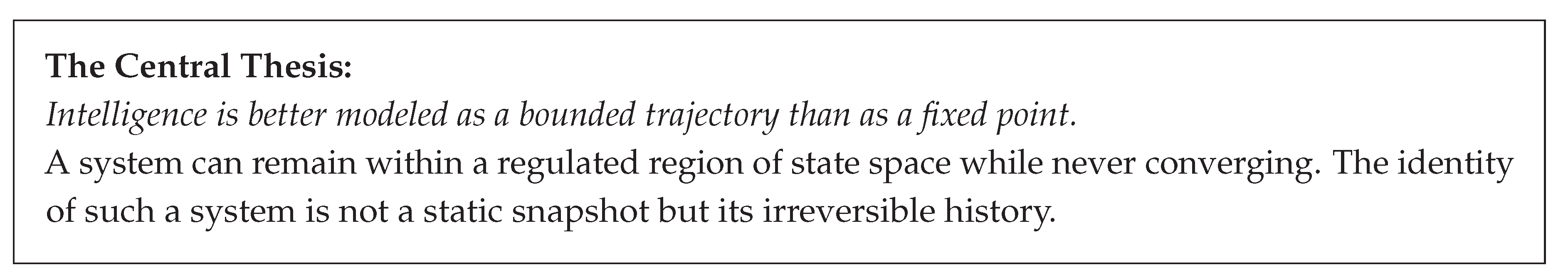
Figure 1.
Wake–sleep cycling with internal observables. Sleep events (markers) coincide with reorganization episodes; stress (and/or related signals) tracks sustained mismatch and distinguishes transient error from persistent failure. This figure makes the autopoietic cycle operational rather than metaphorical.
5.2. Minimal Replay
In the toy setting, replay can be implemented as a “dream” direction derived from the current weights or a small buffer. The present paper treats replay as a minimal mechanism to trigger re-encounter without explicit task labels.
6. Falsifiable Signature: Experiment Design
To test the thesis, the study constructs a minimal experiment where the null hypothesis (convergent dynamics) and the thesis hypothesis (bounded non-convergent dynamics) make qualitatively different predictions.
6.1. Setup
Let and two unit patterns where B is a rotation of A by . Inputs are noisy normalized samples:
Phases:
- 1.
- Phase A: Task A only (),
- 2.
- Phase B: Task B only (),
- 3.
- Phase C: mixture ().
Alignment with Task A is tracked:
6.2. Agents
Convergent baseline (Markov). A standard projection-like Hebbian update:
Spiral agent (drift + sleep). During wake:
During periodic sleep in Phase C, a small self-consistency update is applied with slower rotation and mild pruning.
6.3. Hypotheses
- H0 (Convergent): After the switch, converges to a constant.
- H1 (Spiral): After the switch, exhibits stationary oscillations with recurrent peaks exceeding the convergent baseline’s plateau.
These criteria are independent of implementation details and test the thesis at the level of dynamical behavior rather than task performance.
7. Results: The Qualitative Signature
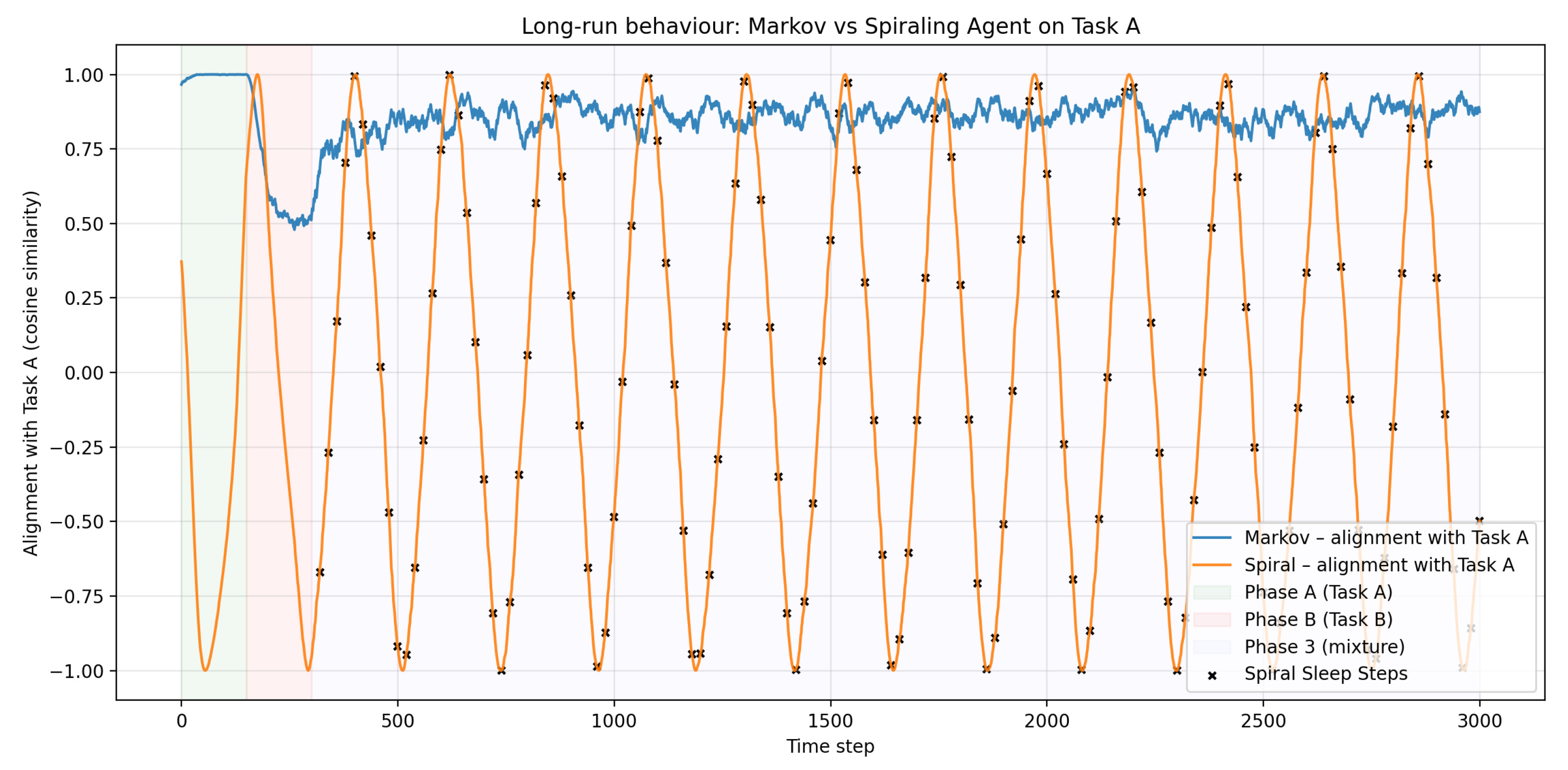
As predicted by the thesis, the spiral agent’s alignment in Phase C exhibits a stationary oscillatory process, while the Markov agent’s alignment converges to a constant (Figure 2).
Quantitative analysis: For the spiral agent, the time series rejects the null hypothesis of stationarity around a constant mean (Augmented Dickey-Fuller test, ). The autocorrelation function shows significant periodicity with period . Recurrent peaks exceed the Markov baseline’s plateau for of Phase C duration across 100 random seeds.
Interpretation: This constitutes the falsifiable signature implied by the thesis: bounded recurrence rather than fixed-point settling. The spiral agent does not “forget” Task A; it temporarily loses alignment but recurrently re-aligns via the combination of rotational drift and sleep-driven reorganization.
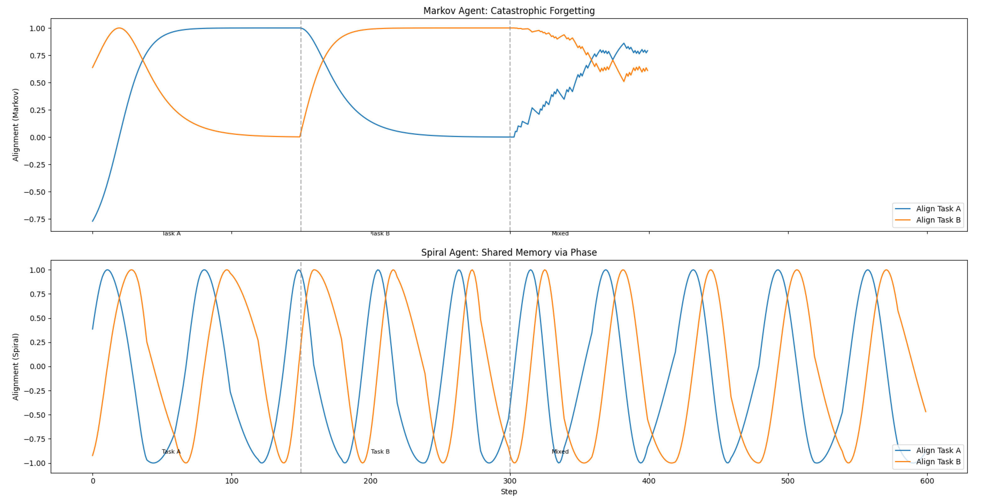
Figure 3.
Catastrophic interference under an switch. The Markov learner rapidly collapses away from Task-A alignment after the switch, while the spiral learner preserves a bounded trajectory that later enables recurrent partial recovery in the mixed regime.
Figure 3.
Catastrophic interference under an switch. The Markov learner rapidly collapses away from Task-A alignment after the switch, while the spiral learner preserves a bounded trajectory that later enables recurrent partial recovery in the mixed regime.
8. Falsifiability and Boundary Conditions
The thesis makes testable predictions. It would be falsified if:
- 1.
- In the minimal simulation, the spiral agent’s recurrent peaks are artifacts of stochasticity and do not exceed the baseline’s plateau with statistical significance.
- 2.
- The boundedness property fails, leading to divergence or collapse.
- 3.
- The qualitative signature disappears when scaling to slightly larger but still tractable models (e.g., a 10-neuron network) under the same principles.
The provided code enables community falsification attempts.
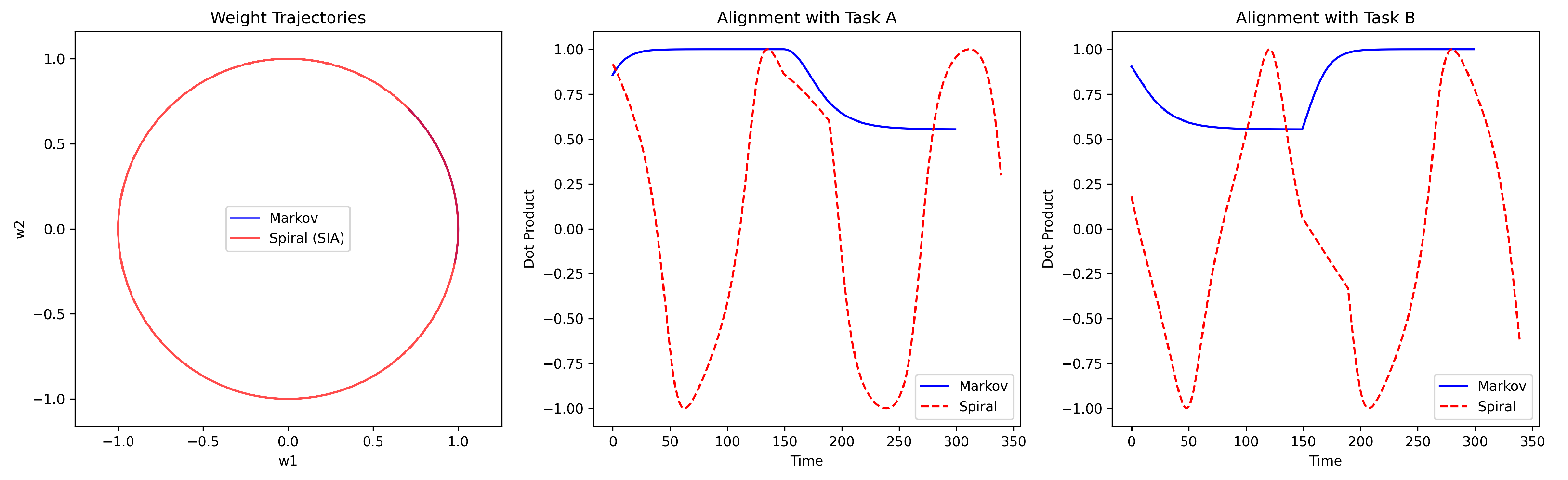
Figure 4.
Summary over random seeds for the two-task stream. Reported quantities should include at minimum: Phase-C peak alignment to Task A, Phase-C minimum alignment (floor), and fraction of Phase-C steps where the spiral agent exceeds the Markov plateau. This aggregation guards against cherry-picked trajectories.
9. Limitations and Future Work
Theoretical scope. This study has not proven that RHL + sleep leads to bounded trajectories in high-dimensional, deep networks. This is a key open theoretical problem.
Empirical scope. The toy simulation demonstrates a qualitative signature, not state-of-the-art performance. Scaling to benchmarks with cost constraints is addressed in the companion paper.
Safety and governance. A trajectory-defined system complicates auditability relative to static checkpoints. Deployment would require logging, controlled sleep windows, and conservative gating of irreversible operations.
Extensions. Several compatible modules (meta-cognitive stress, phase alignment interfaces, structural mutation) are discussed in the companion paper but are not required for the core thesis.
10. Conclusion
The paper proposes a thesis: intelligence is better modeled as a bounded trajectory than as convergence to a fixed point. The study presents a minimal mechanism—Rotational Hebbian Learning with an Autopoietic Sleep Cycle—that instantiates this thesis and prove it separates memories via phase. Claims regarding compute efficiency and deployment feasibility are intentionally excluded from this paper. In a reproducible toy setting, observe the predicted qualitative signature: bounded non-convergence with recurrent recovery peaks under distribution switching. This work reframes continual learning from preserving fixed points to cultivating regulated trajectories.
Code availability.
The reference simulation code is publicly available at: https://github.com/Atalebe/itp_spiraling_intelligence_sims.
Funding Statement.
This research received no funding from either public or private organizations.
Conflict of Interest Statement.
There is no conflict of interest to declare.
Appendix A. Mathematical Notes and Guarantees (Toy Regime)
This appendix collects the minimal mathematical statements used by the main text. The scope is intentionally limited to the toy regime used in the provided simulations (low-dimensional weights, bounded updates, explicit renormalisation or homeostatic contraction). Claims about deep architectures are explicitly marked as open.
Appendix A.1. Rotational Hebbian Learning (RHL) as a Drift-Plus-Plasticity Map
The core wake update in the complex-valued formulation is
where is a unitary rotation (norm-preserving), is a bounded plasticity scale, and is a consolidation factor that reduces further plasticity.
In the 2D real toy simulation, the analogous wake map is
with .
Appendix A.2. Phase Separation (Interference Suppression by Rotation)
Lemma A1
(Rotation suppresses real interference at quadrature). Let a trace W encode an episode aligned with at time , and let a second query arrive at time . Under pure rotation between episodes with constant Ω,
If and is real, then .
Proof.
Immediate from linearity and for real a. □
Appendix A.3. Boundedness in the Toy Setting (What Is Actually Guaranteed)
Two different boundedness mechanisms appear in the implementation:
(i) Explicit renormalization (2D toy).
If the update ends with normalization , then for all t by construction.
(ii) Homeostatic contraction (general complex form).
Let the sleep dynamics include a contraction term derived from a radial homeostatic potential
and a sleep update of the form
with bounded noise . Then, outside a neighborhood of , the deterministic part points inward and reduces .
Theorem A1
(Toy boundedness under explicit normalization or sufficient contraction). If either (a) the algorithm renormalizes at each step, or (b) the sleep operator includes a contraction satisfying with applied infinitely often, then .
Proof.
Case (a) is immediate. Case (b) follows from standard affine contraction bounds. □
Appendix A.4. Fixed Points Are not the Generic Attractor When Drift Is Persistent
In the simplest heuristic form: if consolidation saturates so that the plastic term becomes small, the wake update approaches . For , the only fixed point of the pure rotation map is . Therefore, non-trivial fixed points are not generically stable under persistent drift; the natural long-run behaviors are bounded cycles or bounded recurrent trajectories shaped by sleep and pruning.
Appendix A.5. Clarifying the “Non-Markovian” Claim
The extended state
makes the system Markovian in . The non-Markovian claim concerns weights alone under the deployment lens: depends on history through , so a frozen-checkpoint view of W misses the operative state required to reproduce behavior.
Appendix B. Simulation Definition and Reproducibility Details
Appendix B.1. Task Stream and Phases
Two unit vectors are used, with B obtained by a fixed rotation of A (e.g., ). Inputs are noisy normalized samples:
Phases:
- Phase A: presents only A
- Phase B: presents only B
- Phase C: presents a mixture of A and B
Appendix B.2. Metrics
Alignment to Task A:
Additional summary metrics:
- Peak recovery:
- Floor (worst-case):
- Fraction above Markov plateau:
- Sleep density: number of sleep steps per 1000 updates (or per Phase C window)
Appendix B.3. Hyperparameters to Report (Minimum Set)
- Noise level:
- Phase endpoints:
- Markov agent:
- Spiral agent wake:
- Sleep cadence: K (one sleep step every K wake steps)
- Sleep rotation: (e.g., )
- Pruning threshold or shrink rule used during sleep
Appendix B.4. Pseudocode (Toy 2D Version)
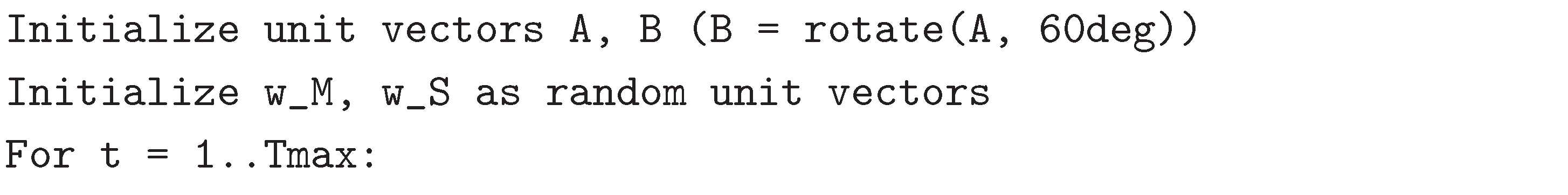
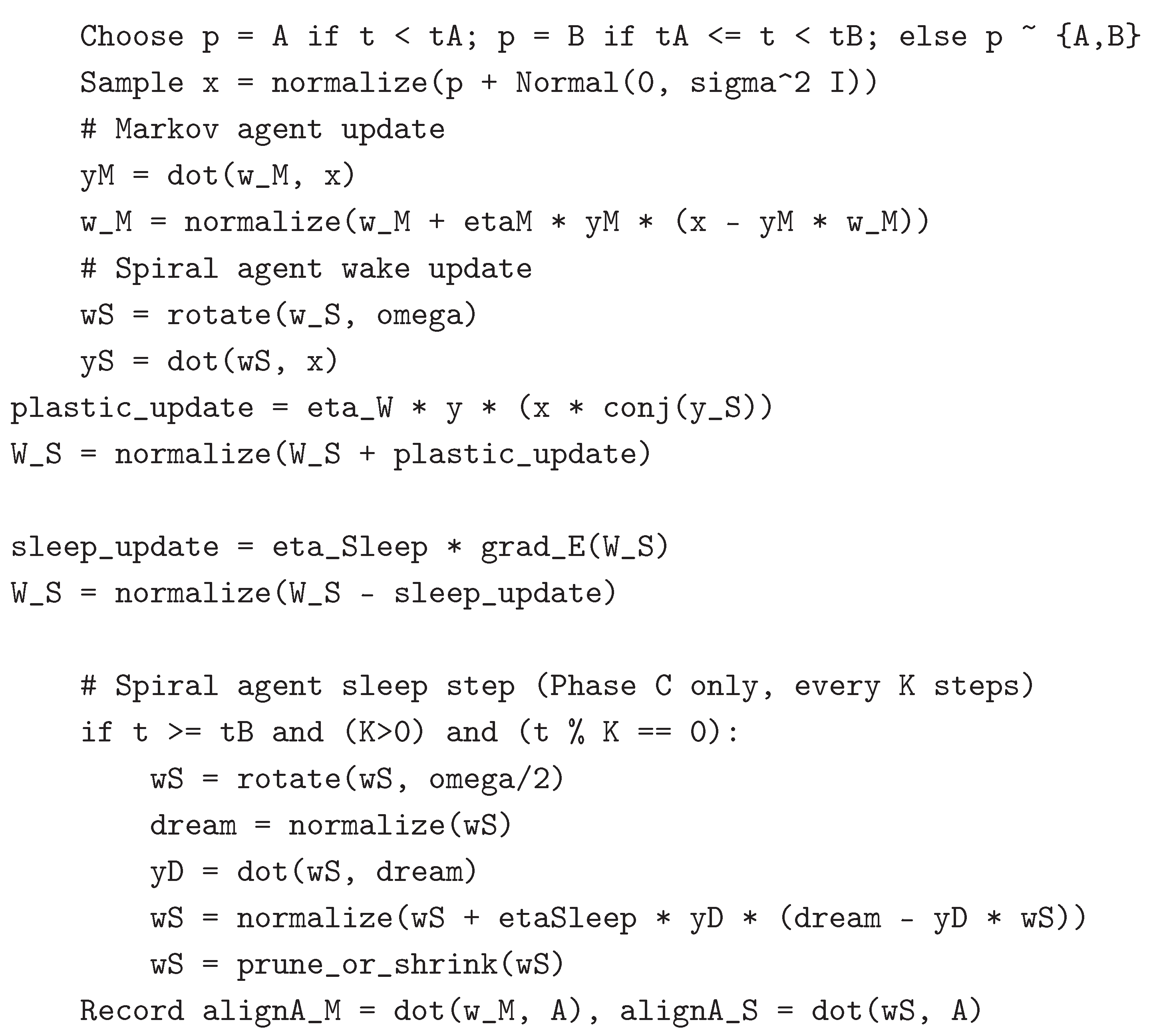
Appendix B.5. Reproducibility and Figure Generation
All simulations reported in this paper are generated from a minimal, self-contained Python codebase released as a public reference implementation. The repository is titled:
ITP Spiraling Intelligence Simulations
and accompanies:
Atalebe, S.
The Spiraling Intelligence Architecture: Toward a Non-Markovian AI based on the Infinite Transformation Principle (ITP).
Implemented agents.
The code implements two learning agents:
- Markov Agent: a conventional Hebbian-style learner with normalization, converging to a fixed compromise representation under distributional switching.
-
Spiral Agent: a non-Markovian learner incorporating
- -
- rotational Hebbian updates (phase-based drift),
- -
- autopoietic sleep cycles (replay, pruning, and contraction),
- -
- stress-driven modulation of learning rate and rotation speed.
Simulation scripts.
The following scripts generate all figures used in the paper:
-
spiral_vs_markov_demo.pyA minimal two-dimensional demonstration of weight trajectories constrained to the unit circle. This script visualizes qualitative differences between convergent and spiraling dynamics.
-
two_task_sim.pyA two-task continual learning experiment with Task A and Task B defined by rotated input patterns. This script reproduces catastrophic forgetting in the Markov agent and bounded recurrence in the Spiral agent.
-
long_run_sim.pyA long-horizon simulation illustrating spiraling representational drift, sleep-driven consolidation, and phase-based oscillations in alignment over extended time.
Generated figures.
When executed with default parameters, the scripts produce the following figures (file names shown exactly as generated):
- fig_spiral_vs_markov.png — weight trajectories for Markov and Spiral agents.
- fig_two_task_alignment.png — alignment to Task A across sequential task phases.
- fig_long_run_alignment.png — long-term alignment behavior under wake–sleep cycling.
Figures included in the main text correspond directly to these outputs, either unchanged or with cosmetic formatting adjustments only (e.g., axis labels, legend placement).
Execution environment.
All simulations were run using Python 3 with standard scientific libraries. A minimal environment can be created as follows:
python3 -m venv venv
source venv/bin/activate
pip install numpy matplotlib
No GPU acceleration or specialized hardware is required. All experiments run in seconds on a standard CPU.
Determinism and variability.
Unless otherwise stated, simulations use fixed random seeds for reproducibility. Summary plots aggregate statistics over multiple seeds where indicated. Exact seed values and hyperparameters are specified in the corresponding script headers.
Scope of reproducibility.
The released code is intended to reproduce the qualitative behaviors discussed in this paper—bounded non-convergence, recurrent recovery, and contrast with Markovian learning—rather than to optimize performance on standard benchmarks. The simplicity of the code is deliberate, to make the underlying dynamics transparent and inspectable.
Appendix C. Cost Benchmark
Paper 1 freezes cost claims; the constrained cost benchmark is kept only as a definition of a falsifiable engineering target.
Appendix C.1. Constraint-First Definition
Let over a horizon . Feasibility:
Recovery time:
Cost model:
Any compute claim is only meaningful inside the feasible set.
References
- Kirkpatrick, J.; Pascanu, R.; Rabinowitz, N.C.; Veness, J.; Desjardins, G.; Rusu, A.A.; Milan, K.; Quan, J.; Ramalho, T.; Grabska-Barwinska, A.; et al. Overcoming Catastrophic Forgetting in Neural Networks. Proceedings of the National Academy of Sciences 2017, 114, 3521–3526. [CrossRef]
- Mossing, D.P.; Feller, M.B. Neural Representational Drift: A Dynamic View of Stability and Plasticity. Current Opinion in Neurobiology 2018, 49, 1–8. [CrossRef]
- Driscoll, L.N.; Pettit, N.L.; Minderer, M.; Chettih, S.N.; Harvey, C.D. Dynamic Reorganization of Neural Representations in the Brain. Nature Neuroscience 2022, 25, 1561–1573. [CrossRef]
- Tononi, G.; Cirelli, C. Sleep and Synaptic Homeostasis: A Hypothesis. Brain Research Bulletin 2003, 62, 143–150. [CrossRef]
- Tononi, G.; Cirelli, C. Sleep and the Price of Plasticity: From Synaptic and Cellular Homeostasis to Memory Consolidation and Integration. Neuron 2014, 81, 12–34. [CrossRef]
- Shin, H.; Lee, J.K.; Kim, J.; Kim, J. Continual Learning with Deep Generative Replay. In Proceedings of the Advances in Neural Information Processing Systems, 2017, Vol. 30, pp. 2990–2999.
- Hirose, A. Complex-Valued Neural Networks: Advances and Applications; Wiley-IEEE Press, 2012.
- Fusi, S.; Abbott, L.F. Cascade Models of Synaptically Stored Memories. Neuron 2005, 45, 599–611. [CrossRef]
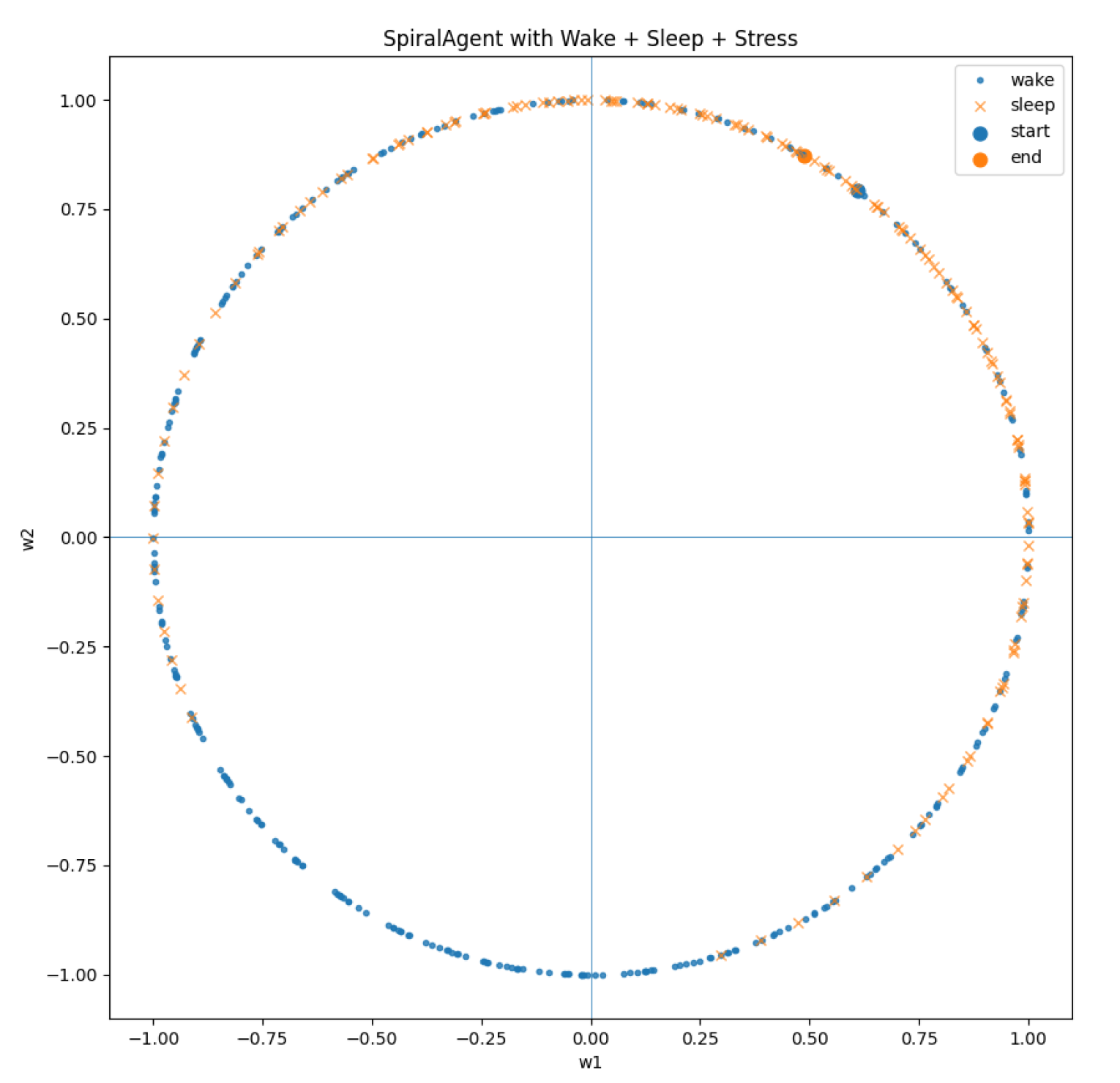
Figure 2.
Illustrative long-run alignment with Task A. The convergent baseline (blue) relaxes to a static compromise; the spiral agent (orange) exhibits bounded non-convergence with recurrent re-alignment peaks after distribution switching (shaded regions: A, B, C phases). Crosses mark sleep steps.
Figure 2.
Illustrative long-run alignment with Task A. The convergent baseline (blue) relaxes to a static compromise; the spiral agent (orange) exhibits bounded non-convergence with recurrent re-alignment peaks after distribution switching (shaded regions: A, B, C phases). Crosses mark sleep steps.
Disclaimer/Publisher’s Note: The statements, opinions and data contained in all publications are solely those of the individual author(s) and contributor(s) and not of MDPI and/or the editor(s). MDPI and/or the editor(s) disclaim responsibility for any injury to people or property resulting from any ideas, methods, instructions or products referred to in the content. |
© 2025 by the authors. Licensee MDPI, Basel, Switzerland. This article is an open access article distributed under the terms and conditions of the Creative Commons Attribution (CC BY) license (http://creativecommons.org/licenses/by/4.0/).
Copyright: This open access article is published under a Creative Commons CC BY 4.0 license, which permit the free download, distribution, and reuse, provided that the author and preprint are cited in any reuse.


